Conditional Random Fields

Rahul Gupta

(KReSIT, IIT Bombay)

Undirected models

• Graph representation of random variables

• Edges define conditional independence statements

• Graph separation criteria• Markovian independence

statements are enough P(S|V) = P(S|Nb(S))

X Y

Z

W

X indep. of W given Z

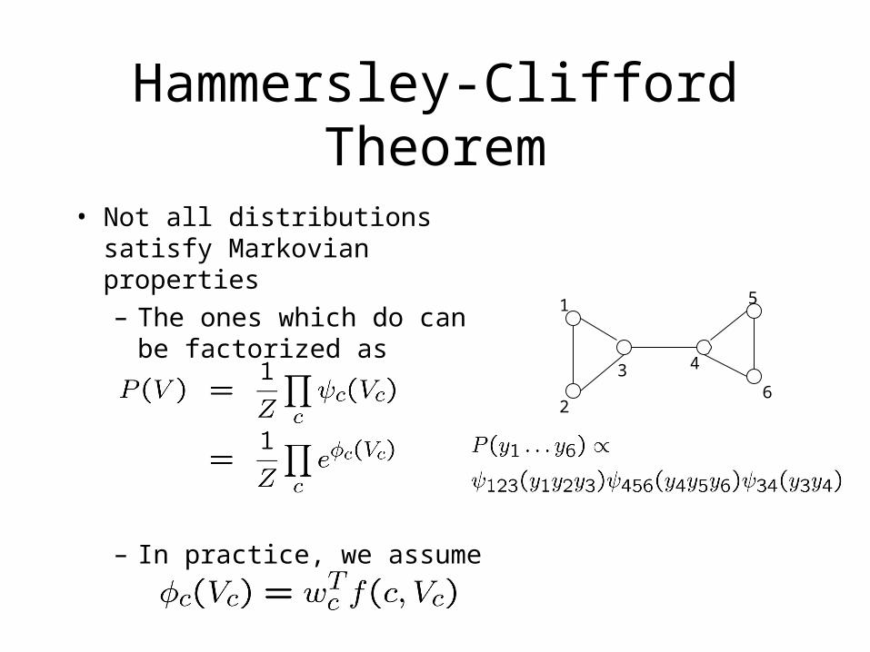
Hammersley-Clifford Theorem

• Not all distributions satisfy Markovian properties– The ones which do can be

factorized as

– In practice, we assume

1

2

5

436

Computing marginals

• We are interested in– Marginals P(S)– Conditionals P(S|S’) = P(S,S’)/P(S’)

• Same as computing marginals

– Labelings with highest joint probabilities• Reuse the algorithm for computing marginals

• Only compute marginals for cliques

Marginals in trees

• Sum-Product Algorithm– Receive belief

messages from children– Pass consolidated belief

to parent

– Node marginal prop. to• Messages from children• Node potential

m21(y1) m31(y1)1

2 3

Marginals (contd.)

• Reuse messages for other marginals

• Running time dependent on tree diameter

• For best labeling, replace sum by max

– Store argmax along with max

Junction-Tree algorithm

• Sum-Product fails to converge with cycles– Make graph acyclic by merging cliques– Run Sum-Product on

transformed graph– Local consistency

• Runtime exponential in max clique size

1

2

5

436

1’ 2’ 3’

1’(y1’)= 1(y1)2(y2)12(y1y2)23(y2y3)13(y1y3)

2’(y2’) = 3(y3)4(y4)34(y3y4)

Junction-Tree (contd.)

• Blindly arranging cliques is wrong– Message Passing

maintains only local consistency

– Need a ‘running intersection property’

2

1

35

4

124

25

234

124

25

234

Junction treeP(4) may not be consistent

Junction Tree (contd.)

• Junction-Tree cannot exist for un-triangulated graphs– Triangulate the graph– Max clique size may increase

arbitrarily– NP-hard to output the best

triangulation

2

1

3

4

12

23

34

14

P(1) not consistent

ILP-based inferencing

• c(yc) is 1 if clique c has value yc

• c(yc)’s are mutually exclusive

• c(yc) and c’(yc’) are consistent for c’ ½ c

• LP relaxation– c(yc) behave like marginal probabilities

– May admit invalid solutions if the graph is un-triangulated!

• Triangulation adds variables and constraints that keep the solution valid

Approximate inferencing

• Sampling-based methods

• Variational methods– Find upper and lower bounds to marginals

• Approximate algos when potentials are metrics (Kleinberg, Tardos 99)– O(logk loglogk) approx ratio for k labels– 2-approx algo for uniform potentials

Learning the potentials

Max-margin formulation

• Assume– Triangulated graph, one node x is fixed

• x has edges to all nodes

– c(yc) = (yc) = wTf(c,yc,x)• f : vector of arbitrary local features of the clique• w : weights of the features (will be learnt)

• P(y|x) / exp(wTc f(c,yc,x))

– Loss function can be decomposed over cliques

• Given (x,y), ideally we want P(y|x) to be higher than any other P(y’|x)

Max-margin (contd.)

• Exponential number of constraints

• Transform to

• Can use a cutting plane approach

• Still not fully exploiting the decomposability of F and L

Max-margin dual

• ’s occur only as– ’s behave as probability distributions, and

behave like marginals

• However, constraints are not enough if graph is un-triangulated.

Max-margin (contd.)

• Rewrite dual in terms of c(yc)

– Drastic reduction in number of variables.

• Algorithms for solving the dual– Modified SMO– Exponentiated gradient algorithm

SMO

• For example i:– Pick y’ and y’’ using KKT violations

• e.g. i,y’ = 0 but (i,y’) is a support vector

• i,y’ and i,y’’ will be optimized

• But ’s are neither known, nor unique – Use maximum entropy principle

– Closed form optimization for chosen ’s• Let be the mass transfer from i,y’ to i,y’’

SMO (contd.)

• Project back the changes to relevant ’s– i,c(yc) receives mass if yc is a part of y’

– i,c(yc) loses mass if yc is a part of y’’

– Both may happen to the same marginal variable

Exponentiated Gradient

• Exponentiated updates

• Normalization ) simplex constraint.

• exp() ) non-negativity• r = grad of the dual objective

• Cannot update explicitly– Use the decomposability of F and L

Exponentiated Gradient

• Parameterize ’s

) gradient descent for ’s

• Gradient should not have ’s– Tricky term is – This is the ‘expectation’

• Replace sums over ’s by local marginals• Expectation becomes

Exponentiated Gradient (contd.)

• Marginals can be computed quickly using message passing

• Final algo 1. Begin with some random ’s2. Compute marginals 3. Compute gradient using 4. Update ’s, goto Step 2

• Exponentiated gradient experimentally shown to be better than SMO

Other training methods

• Maximize log-likelihood (log P(y|x))• Maximize pseudo-likelihood (ilogP(yi|x))

– Useful for Hamming loss functions

• Voted perceptron– Approximate the gradient of log-likelihood

• Piecewise training– Divide the graph into independently normalized parts

• Gradient tree boosting• Logarithmic pooling

– Learn a committee of simpler CRFs

Associative Markov Networks

• Potentials favour same labeling of all vertices in the clique– c(yc) = k fc(k)« y

c = (k,…,k) ¬

– Hypertext classification, Image segmentation

• Instead of c(yc), we have c(k) which is one for labeling the clique with k– Training is highly simplified

AMNs (contd.)

• Inferencing– LP relaxation is optimal for binary labels

• Can be reduced to graph min-cut

– For multiple labels, use iterative min-cut• At step k, do a min-cut to decide whether nodes keep

their labels or switch to label k

• Approx algo with O(logk loglogk) ratio if potentials are metric

• 2-approx algo if potentials are uniform and metric

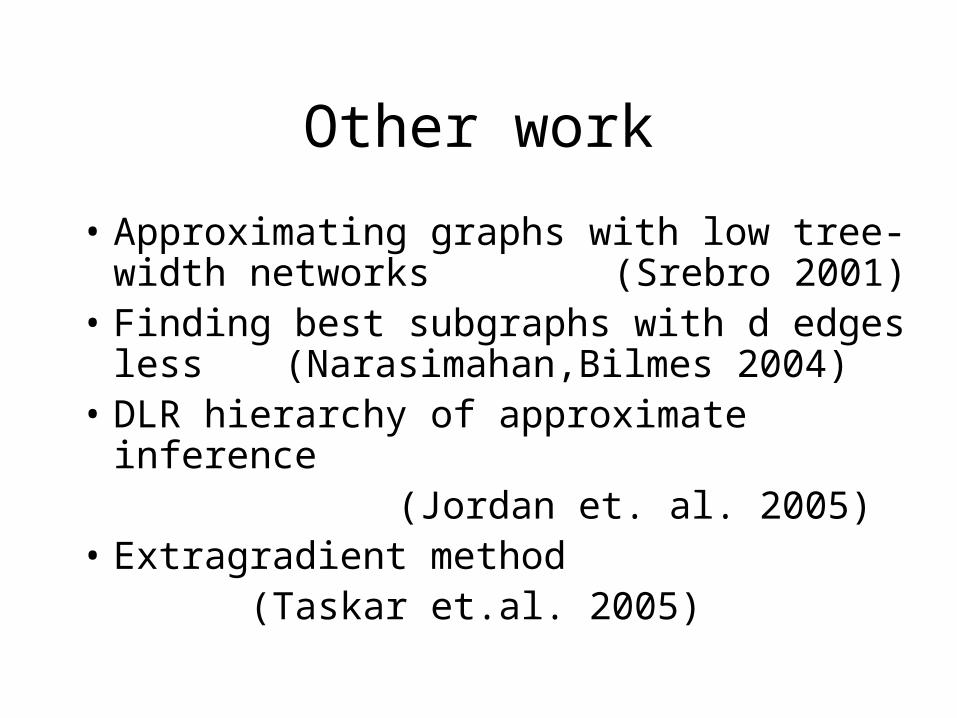
Other work

• Approximating graphs with low tree-width networks (Srebro 2001)

• Finding best subgraphs with d edges less (Narasimahan,Bilmes 2004)

• DLR hierarchy of approximate inference (Jordan et. al. 2005)

• Extragradient method (Taskar et.al. 2005)

Possible directions

• Integrating CRFs with imprecise DBs– CRF probabilities interpretable as confidence – Compress exponential number of outputs– Exploit Markovian property

• Piecewise training– Label bias / loss of correlation vs efficiency

• Constrained inferencing– Probabilities lose interpretability ?