Conditional Skewness in Asset Pricing Testscharvey/Teaching/CDROM_BA456_200… · Conditional Skewness in Asset Pricing Tests ... tum portfolios have higher skewness ... turns more

Conditional Skewness in Asset Pricing Tests

CAMPBELL R. HARVEY and AKHTAR SIDDIQUE*

ABSTRACT

If asset returns have systematic skewness, expected returns should include re-wards for accepting this risk. We formalize this intuition with an asset pricingmodel that incorporates conditional skewness. Our results show that conditionalskewness helps explain the cross-sectional variation of expected returns acrossassets and is significant even when factors based on size and book-to-market areincluded. Systematic skewness is economically important and commands a riskpremium, on average, of 3.60 percent per year. Our results suggest that the mo-mentum effect is related to systematic skewness. The low expected return momen-tum portfolios have higher skewness than high expected return portfolios.

THE SINGLE FACTOR CAPITAL ASSET PRICING MODEL ~CAPM! of Sharpe ~1964! andLintner ~1965! has come under recent scrutiny. Tests indicate that the cross-asset variation in expected returns cannot be explained by the market betaalone. For example, a growing number of studies show that “fundamental”variables such as size, book-to-market value, and price to earnings ratiosaccount for a sizeable portion of the cross-sectional variation in expectedreturns ~see, e.g., Chan, Hamao, and Lakonishok ~1991! and Fama and French~1992!!. Fama and French ~1995! document the importance of SMB ~the dif-ference between the return on a portfolio of small size stocks and the returnon a portfolio of large size stocks! and HML ~the difference between thereturn on a portfolio of high book-to-market value stocks and the return ona portfolio of low book-to-market value stocks!.

There are a number of responses to these empirical findings. First, thesingle-factor CAPM is rejected when the portfolio used to proxy for the mar-ket is inefficient ~see Roll ~1977! and Ross ~1977!!. Roll and Ross ~1994! andKandel and Stambaugh ~1995! show that even very small deviations fromefficiency can produce an insignificant relation between risk and expectedreturns. Second, Kothari, Shanken, and Sloan ~1995! and Breen and Korajczyk~1993! argue that there is a survivorship bias in the data used to test thesenew asset pricing specifications. Third, there are several specification issues.Kim ~1995! and Amihud, Christensen, and Mendelson ~1993! argue that errors-in-variables impact the empirical research. Kan and Zhang ~1997! focus ontime-varying risk premia and the ability of insignificant factors to appear

* The authors are from Duke University and Georgetown University respectively. We appre-ciate the comments of Philip Dybvig, Stephen Brown, Alon Brav, S. Viswanathan, and seminarparticipants at Georgetown, Indiana University, the University of Toronto, the 1996 WFA ~Oregon!,and the AFA ~New Orleans! meetings. We appreciate the helpful comments of an anonymousreferee and the detailed suggestions of the editor.

THE JOURNAL OF FINANCE • VOL. LV, NO. 3 • JUNE 2000

1263

significant as a result of low-powered tests. Jagannathan and Wang ~1996!show that specifying a broader market portfolio can affect the results. Fi-nally, Ferson and Harvey ~1998! show that even these new multifactor spec-ifications are rejected because they ignore conditioning information.

The goal of this paper is to examine the linkage between the empiricalevidence on these additional factors and systematic coskewness. The follow-ing is our intuition for including skewness in the asset pricing framework.In the usual setup, investors have preferences over the mean and the vari-ance of portfolio returns. The systematic risk of a security is measured asthe contribution to the variance of a well-diversified portfolio. However, thereis considerable evidence that the unconditional returns distributions cannotbe adequately characterized by mean and variance alone.1 This leads us tothe next moment—skewness. Everything else being equal, investors shouldprefer portfolios that are right-skewed to portfolios that are left-skewed.This is consistent with the Arrow–Pratt notion of risk aversion. Hence, as-sets that decrease a portfolio’s skewness ~i.e., that make the portfolio re-turns more leftskewed! are less desirable and should command higher expectedreturns. Similarly, assets that increase a portfolio’s skewness should havelower expected returns.

One clue that pushed us in the direction of skewness is the fact that someof the empirical shortcomings of the standard CAPM stem from failures inexplaining the returns of specific securities or groups of securities such asthe smallest market-capitalized deciles and returns from specific strategiessuch as ones based on momentum. These assets are also the ones with themost skewed returns. Skewness may be important in investment decisionsbecause of induced asymmetries in ex post ~realized! returns. At least twofactors may induce asymmetries. First, the presence of limited liability in allequity investments may induce option-like asymmetries in returns ~see Black~1972!, Christie ~1982!, Nelson ~1991!, and Golec and Tamarkin ~1998!!. Sec-ond, the agency problem may induce asymmetries in portfolio returns ~seeBrennan ~1993!!. That is, a manager has a call option with respect to theoutcome of his investment strategies. Managers may prefer portfolios withhigh positive skewness.

We present an asset pricing model where skewness is priced. Our formu-lation is related to the seminal work of Kraus and Litzenberger ~1976! andto the nonlinear factor models presented more recently in Bansal andViswanathan ~1993! and Leland ~1997!. We use an asset pricing model in-corporating conditional skewness to help understand the cross-sectional vari-ation in several sets of asset returns.

Our work differs from Kraus and Litzenberger ~1976! and Lim ~1989! inour focus on conditional skewness rather than unconditional skewness aswell as in our objective of explaining the cross-sectional variation in ex-

1 Merton ~1982! shows that if instantaneous returns are normal, then the price process islognormal and, unless the measurement interval is very small, the simple returns are notnormal.

1264 The Journal of Finance

pected returns. Conditional skewness also captures asymmetry in risk, es-pecially downside risk, which has come to be viewed by practitioners asimportant in contexts such as value-at-risk ~VaR!. Our work focuses primar-ily on monthly U.S. equity returns from CRSP. We form portfolios of equitieson various criteria such as industry, size, book-to-market ratios, coskewnesswith the market portfolio ~where we define coskewness as the component ofan asset’s skewness related to the market portfolio’s skewness!, and momen-tum using both monthly holding periods as well as longer holding periods.Additionally, we also examine individual equity returns.

We analyze the ability of conditional coskewness to explain the cross-sectional variation of asset returns in comparison with other factors. Wefind that coskewness can explain some of the apparent nonsystematic com-ponents in cross-sectional variation in expected returns even for portfolioswhere previous studies have been unsuccessful. The pricing errors in port-folio returns using other asset pricing models can also be partly explainedusing skewness. Our results, however, show that the asset pricing puzzle isquite complex and the success of a given multifactor model depends sub-stantially on the methodology and data used to empirically test the model.We also find that an important role is played by the degree of precisioninvolved in computing the asset betas with respect to the factors—that is,what may be a proxy for estimation risk.

Our paper is organized as follows. In Section I, we use a general stochasticdiscount factor pricing framework to show how skewness can affect the ex-pected excess asset returns. We also develop specific implications for theprice of skewness risk based on utility theory. The data used in the paperand summary statistics are in Section II. Section III contains the economet-ric methodology and empirical results. Some concluding remarks are offeredin Section IV.

I. Skewness in Asset Pricing Theory

The first-order condition for an investor holding a risky asset ~in a repre-sentative agent economy! for one period is

E @~1 1 Ri, t11!mt116Vt # 5 1, ~1!

where ~1 1 Ri, t11! is the total return on asset i, mt11 is the marginal rate ofsubstitution of the investor between periods t and t 1 1, and Vt is the in-formation set available to the investor at time t. The marginal rate of sub-stitution mt11 can be viewed as a pricing kernel or a stochastic discountfactor that prices all risky asset payoffs.2

2 See Harrison and Kreps ~1979!, Hansen and Richard ~1987!, Hansen and Jagannathan~1991!, Cochrane ~1994!, Carhart et al. ~1994!, and Jagannathan and Wang ~1996!.

Conditional Skewness in Asset Pricing Tests 1265

Under no arbitrage, the discount factor in equation ~1!, mt11, must benonnegative ~see Harrison and Kreps ~1979!!. The marginal rate of substi-tution is not observable. Hence, to obtain testable restrictions from this first-order condition, we need to define observable proxies for the marginal rateof substitution. Different asset pricing models differ primarily in the proxiesthey use for the marginal rate of substitution and the mechanisms they useto incorporate the proxies into the asset pricing model. The proxies can beeither observed returns of financial assets such as equity portfolios or non-market variables such as growth rate in aggregate consumption as in Hansenand Singleton ~1983!. The form and specification of the marginal rate ofsubstitution is determined jointly by the assumptions about preferences anddistributions of the proxies. A specification for the marginal rate of substi-tution can also be viewed as a restriction on the set of trading strategiesthat the marginal investor can use to achieve the utility-maximizing port-folios. Thus, the standard capital asset pricing model implies that the opti-mal trading strategy for the marginal investor is to invest in the risk-freerate and the market portfolio.

A. A Three-Moment Conditional CAPM

In the traditional CAPM, one of two routes is usually pursued. In a two-period world with homogeneous agents, the representative agent’s derivedutility function ~in wealth! may be restricted to forms such as quadratic orlogarithmic which guarantee that the discount factor is linear in the value-weighted portfolio of wealth. The other route involves making distributionalassumptions on the asset returns, such as the elliptical class, which alsoguarantees that the discount factor is linear in the value-weighted portfolioof wealth. The empirical predictions ~i.e., restrictions on the moments of thereturns! are identical in either case. The assumption that the marginal rateof substitution is linear in the market return,

mt11 5 at 1 bt RM, t11, ~2!

produces the classic CAPM with the weights at and bt being functions ofperiod-t information set. To see this, expand the expectation in equation ~1!:

Covt @mt11, ~1 1 Ri, t11!# 1 Et @1 1 Ri, t11#Et @mt11# 5 1, ~3!

which can also be written as

Et @1 1 Ri, t11# 51

Et @mt11#2

Covt @mt11, ~1 1 Ri, t11!#

Et @mt11#. ~4!


Assuming the existence of a conditionally risk-free asset and given equation~2!, we get the standard CAPM

Et @ri, t11# 5Covt @ri, t11, rM, t11#

Vart @rM, t11#Et @rM, t11#

or

Et @ri, t11# 5 bi, t Et @rM, t11# , ~5!

where r represents returns in excess of the conditionally risk-free return.This expression decomposes the expected excess return into the product ofthe asset’s beta and the market risk premium. The econometric restrictionsuch a model imposes is that in a time-series regression of the excess re-turns on the market excess return, the intercept should be zero, the betasshould be significant, and the market risk premium estimate should be thesame across all the assets. In a cross-sectional regression of the excess re-turns on the betas, the slope, the market risk premium, should be signifi-cantly different from zero.

An alternative to the linear specification is to assume that the marginalrate of substitution is nonlinear in its observed proxies. Here we are con-fronted with the large number of choices for nonlinear functions, each ofwhich implies a different restriction on the marginal investor’s trading strat-egies. We assume that the stochastic discount factor is quadratic in the mar-ket return; that is,

mt11 5 at 1 bt RM, t11 1 ct RM, t112 . ~6!

We choose the quadratic form because we show later that the quadratic formcan be linked to an important property that all admissible utility functionsmust have. Additionally, it also is one of the simplest types of nonlineari-ties.3 The quadratic form for the marginal rate of substitution implies anasset pricing model where the expected excess return on an asset is deter-mined by its conditional covariance with both the market return and thesquare of the market return ~conditional coskewness!.

Bansal and Viswanathan ~1993! assume that the marginal rate of substi-tution is nonlinear in several factors and they directly test the first-ordercondition on the marginal rate of substitution; however, they do not haveexplicit expressions for premia for the risk factors in their model. In con-trast, our approach involves a similar initial assumption that the marginal

3 We can derive this expression for the marginal rate of substitution ab initio using severaldifferent models of preferences and return distributions or by using a second-order Taylor ex-pansion of the marginal rate of substitution. Alternatively, a two-period model with asymmetricreturn distribution will also produce the same expression. For example, expected utility max-imization in an infinite-horizon economy of representative agents with logarithmic preferencesand an asymmetric return distribution will produce the expression for the marginal rate ofsubstitution that includes RM, t11

2 .


rate of substitution is a nonlinear function of market, SMB, and HML. How-ever, with an explicit functional form for the marginal rate of substitution,we derive explicit expressions for risk premia. Additionally, our formulationpermits us to accommodate nonincreasing absolute risk aversion. Nonin-creasing absolute risk aversion ~i.e., risk aversion should not increase if wealthincreases! is a property that all utility functions should have. This propertycan be explicitly modeled as skewness in a two-period model.

Assuming the existence of a conditionally risk-free asset, we obtain

Et @ri, t11# 5 l1, t Covt @ri, t11, rM, t11# 1 l2, t Covt @ri, t11, rM, t112 # ~7a!

where

l1, t 5Vart @rM, t11

2 #Et @rM, t11# 2 Skewt @rM, t11#Et @rM, t112 #

Vart @rM, t11#Vart @rM, t112 # 2 ~Skewt @rM, t11# !2 , ~7b!

l2, t 5Vart @rM, t11#Et @rM, t11

2 # 2 Skewt @rM, t11#Et @rM, t11#

Vart @rM, t11#Vart @rM, t112 # 2 ~Skewt @rM, t11# !2 . ~7c!

The restriction this model imposes on a cross-section of assets is that l1, tand l2, t are the same across all the assets and are statistically differentfrom zero. This is the conditional version of the three-moment CAPM firstproposed by Kraus and Litzenberger ~1976! who use a utility function de-fined over the unconditional mean, standard deviation, and the third root ofskewness.4 Rewriting equation ~7! as

Et @ri, t11# 5 At Et @rM, t11# 1 Bt Et @rM, t112 # , ~8!

where At and Bt are functions of the market variance, skewness, covariance,and coskewness, illustrates the relation between our model and the Krausand Litzenberger three-moment CAPM. At and Bt are analogous to the betain the traditional CAPM.5 Equation ~8! is an empirically testable restrictionimposed on the cross section of expected asset returns by the asset pricingmodel incorporating skewness, and as such it is an alternative to equation ~5!.

The empirical studies of asset pricing may be seen as attempts to find thebest among these competing specifications of the pricing kernel. However, itis also possible that no one model solves the asset pricing puzzle and differ-

4 Also see Friend and Westerfield ~1980! and Ingersoll ~1990!. Alternative models with threemoments are used by Sears and Wei ~1985!, Nummelin ~1994!, Lim ~1989!, and Waldron ~1990!.Coskewness could also be important for hedging the volatility shocks to the market portfolio asshown by Racine ~1995!.

5 Another simple nonlinearity is to assume that the marginal investor’s trading strategiesare restricted to the risk-free asset and a call option on the market. This produces the Bawaand Lindenberg ~1977! asset pricing model.


ent combinations of factors work for different settings. Therefore, we con-sider an asset pricing model that is a combination of the multifactor modelalong with a simple nonlinear component derived from skewness. Our choiceis also consistent with the findings in Ghysels ~1998! that nonlinear multi-factor models are more successful empirically than linear beta models.

B. How Skewness Enters Asset Pricing

The various asset pricing specifications can also be viewed as competingapproximations for the discount factor or the intertemporal marginal rate ofsubstitution. The nonmarket variables in equations ~7! or ~8! may also beviewed as proxies for the hedge portfolios ~information about future returns!in a dynamic model such as that of Campbell ~1993!. If we relate the dis-count factor to the marginal rate of substitution between periods t and t 1 1,in a two-period economy, a Taylor’s series expansion allows us to make thefollowing identification:

mt11 5 1 1Wt U

''~Wt !

U '~Wt !RM, t11 1 o~Wt !, ~9!

where o~Wt ! is the remainder in the expansion and Wt U''~Wt !0U

'~Wt !, whichis 2bt in equation ~2!, is relative risk aversion. Then at 5 1 1 o~Wt ! andbt , 0. A negative bt implies that with an increase in next period’s marketreturn, the marginal rate of substitution declines. This decline in the mar-ginal rate of substitution is consistent with decreasing marginal utility.

In a similar fashion we assume that the pricing kernel is quadratic in themarket return, that is, mt11 5 at 1 bt RM, t11 1 ct RM, t11

2 . Expanding, asbefore, the marginal rate of substitution in a power series gives

mt11 5 1 1Wt U

''~Wt !

U '~Wt !RM, t11 1

Wt2 U '''~Wt !

2U '~Wt !RM, t11

2 1 o~Wt !. ~10!

Then bt , 0 and ct . 0 since nonincreasing absolute risk aversion impliesU ''' . 0.6 According to Arrow ~1964!, nonincreasing absolute risk aversion isone of the essential properties for a risk-averse individual.

Nonincreasing absolute risk aversion for a a risk-averse utility-maximizingagent can also be linked to prudence as defined by Kimball ~1990!. Prudencerelates to the desire to avoid disappointment and is usually linked to theprecautionary savings motive. Nonincreasing absolute risk aversion impliesthat in a portfolio, increases in total skewness are preferred. Since addingan asset with negative coskewness to a portfolio makes the resultant port-

6 Nonincreasing absolute risk aversion implies that its derivative should be less than orequal to zero. U ''' $ 0 is a necessary condition to satisfy this. Also see Scott and Horvath ~1980!for a discussion of the preference of moments beyond variance.


folio more negatively skewed ~i.e., reduces the total skewness of the portfo-lio!, assets with negative coskewness must have higher expected returnsthan assets with identical risk-characteristics but zero-coskewness. Thus, ina cross section of assets, the slope of the excess expected return on condi-tional coskewness with the market portfolio should be negative. Thus, thepremium for skewness risk over the risk-free asset’s return ~assuming thatthe risk-free asset possesses zero betas with respect to all the factors beingexamined to explain the cross section of returns! should also be negative. Inequation ~7! we are able to decompose contributions of conditional covari-ance and coskewness with the market to the expected excess return of aspecif ic asset. Alternative nonlinear frameworks such as Bansal andViswanathan ~1993! are unable to provide this decomposition.

C. The Geometry of Mean-Variance-Skewness Efficient Portfolios

Figure 1, Panel A, presents a mean-variance-skewness surface. Slicing thesurface at any level of skewness, we get the familiar positively sloping por-tion of the mean-variance frontier. Skewness adds the following possibility:at any level of variance, there is a negative trade-off of mean return andskewness. That is, to get investors to hold low or negatively skewed portfo-lios, the expected return needs to be higher. This is evident in the graph.

Panel B of Figure 1 introduces the risk-free rate. The capital market “line”starts out at zero variance–zero skewness. Think of a ray from the risk-freerate ~at zero variance! that is tangent to the surface at a particular variance-skewness combination. For that level of variance, there are many possibleportfolios with different skewnesses. The tangency point is the one with thehighest skewness. Now add another ray from the risk-free rate that is tan-gent to a different variance-skewness point.

In the usual mean variance analysis, there is a single efficient risky-assetportfolio. In the mean-variance-skewness analysis, however, there are mul-tiple efficient portfolios. The optimal portfolio for the investor is chosen asthe tangency of the investor’s indifference surface to the capital market plane.

II. Does Skewness Exist in the Returns Data?—Portfolio Formation and Summary Statistics

For the empirical work, we use monthly U.S. equity returns from CRSPNYSE0AMEX and Nasdaq files. We form portfolios from the equities as wellas analyze individual equity returns. Most of our work focuses on the periodJuly 1963 to December 1993. We use a longer sample to investigate theinteractions of momentum and skewness. As factors capable of explainingcross-sectional variations in excess returns, we use the CRSP NYSE0AMEXvalue-weighted index as the market portfolio. To capture the effects of sizeand book-to-market value, we use the SMB and HML hedge portfolios formedby Fama and French. These portfolios are constructed to capture the


marketwide effect of size and book-to-market value. The average annualizedreturns on these portfolios from July 1963 to December 1993 are 3.5 percentand 5.6 percent respectively.

Table I presents some summary statistics that compare the different mea-sures of coskewness across five portfolio groups. The first group represents32 value-weighted industry portfolios.7 The second set are the 25 portfoliossorted on size and book-to-market value used by Fama and French ~1995,

7 Of the 32 industry portfolios, we exclude five portfolios from the regression because theyinclude fewer than 10 firms. Summary statistics for portfolios constructed on other criteria areavailable from the authors.

Figure 1. A mean–variance–skewness surface. The trade-offs between mean, variance, andskewness are illustrated. The surfaces are generated using a positive trade-off between meanand variance and a negative trade-off between mean and skewness. Panel A presents the sur-face without a risk-free rate. In Panel B, rays are drawn from the risk-free rate to be tangentialto the surface. The tangent points represent efficient portfolios.


Tab

leI

Su

mm

ary

Sta

tist

ics

onP

ortf

olio

sT

his

tabl

esu

mm

ariz

esfo

ur

sets

ofpo

rtfo

lios

form

edfr

omm

onth

lyU

.S.e

quit

yre

turn

s.T

he

mar

ket

port

foli

ois

the

valu

e-w

eigh

ted

NY

SE0A

ME

Xin

dex.

Sta

nda

rdiz

edu

nco

ndi

tion

alsk

ewn

ess

isth

eth

ird

cen

tral

mom

ent

abou

tth

em

ean

.Sta

nda

rdiz

edu

nco

ndi

tion

alco

skew

nes

sof

the

ith

asse

tis

defi

ned

asE

@ei,

te M

,t2

#0%

E@e

i,t

2#E

@eM

,t2

#,w

her

ee t

are

resi

dual

sfr

omre

gres

sin

gth

eex

cess

retu

rnof

asse

ti

onth

em

arke

tre

turn

.T

he

bs

are

com

pute

dfr

omu

niv

aria

tere

gres

sion

sof

the

port

foli

ore

turn

onth

eri

skfa

ctor

.Tim

e-va

riat

ion

inco

ndi

tion

alco

skew

nes

sis

capt

ure

dth

rou

ghth

eau

tore

gres

sion

Et@e

i,t1

1e M

,t1

12

#5

r0

1r

1e i

,te M

,t2

1r

2e i

,t2

1e M

,t2

12

and

wh

eth

erit

issi

gnif

ican

tat

the

10pe

rcen

tle

vel.

Cro

ss-s

ecti

onal

corr

elat

ion

sbe

twee

nth

eav

erag

eex

cess

retu

rns

and

oth

erpo

rtfo

lio-

spec

ific

vari

able

sar

eal

sore

port

ed.

S5

smal

lest

thir

din

size

,M

5m

iddl

eth

ird

insi

ze,

B5

larg

est

thir

din

size

.S

ign

ific

ance

leve

lsfo

ru

nco

ndi

tion

alsk

ewn

ess

and

cosk

ewn

ess

are

com

pute

dby

gen

erat

ing

the

stat

isti

c10

,000

tim

esby

sim

ula

tin

git

un

der

the

nu

ll,

spec

ific

ally

usi

ng

aN

orm

al~0

,1!

for

skew

nes

s,an

dan

AR

MA

~2,0

!pr

oces

su

sin

ga

biva

riat

eN

orm

alfo

rco

skew

-n

ess.

Wit

h36

6ob

serv

atio

ns,

skew

nes

sis

sign

ific

ant

at2

0.25

3an

d0.

254

atth

e5

perc

ent

leve

lan

d2

0.21

0an

d0.

212

atth

e10

perc

ent

leve

l.C

oske

wn

ess

issi

gnif

ican

tat

60.

095

atth

e10

perc

ent

leve

lan

d6

0.10

8at

the

5pe

rcen

tle

vel.

Pan

elA

.P

ortf

olio

sF

orm

edon

Indu

stri

alC

lass

ific

atio

n,

July

1963

–Dec

embe

r19

93

Indu

stry

Sta

nda

rdiz

edU

nco

ndi

tion

alS

kew

nes

s

Sta

nda

rdiz

edU

nco

ndi

tion

alC

oske

wn

ess

bto

S2

-S1

bto

S2

-Rf

bto

~RM

2R

f!2

Tim

e-V

aryi

ng

Cos

kew

nes

s

Ave

rage

Exc

ess

Ret

urn

bto

RM

2R

f

St.

Dev

.

Ext

ract

ive

20.

305*

*2

0.10

2**

20.

518*

*0.

745*

*2

0.01

3*Ye

s0.

642

0.83

4**

5.41

4O

il&

gas

20.

016

20.

032

20.

738*

*0.

746*

*2

0.01

0N

o0.

499

0.87

9**

5.27

6B

uil

din

g&

con

stru

ctio

n0.

037

0.10

3**

20.

058

1.22

3**

20.

010

No

0.46

71.

278*

*6.

257

Ch

emic

als

20.

258*

*2

0.00

30.

043

0.95

3**

20.

010

Yes

0.40

20.

976*

*4.

723

Com

pute

rs,

elec

tric

al&

elec

tron

ics

&el

ectr

onic

equ

ipm

ent

20.

140

0.10

3**

0.07

91.

040*

*2

0.00

8Ye

s0.

377

1.06

5**

5.35

5E

ngi

nee

rin

g—P

rim

ary

met

als,

mac

hin

ing

20.

364*

*2

0.15

7**

20.

230*

1.05

8**

20.

015*

Yes

0.36

31.

129*

*5.

551

Veh

icle

s0.

052

20.

230*

0.22

10.

934*

*2

0.02

0**

No

0.46

10.

941*

*5.

914

Pap

er,

pulp

,&

prin

tin

g0.

476*

*0.

063

20.

078

1.01

0**

20.

009

Yes

1.07

11.

056*

*6.

644

Text

iles

&ap

pare

l2

0.28

4**

20.

204*

*0.

127

1.13

0**

20.

019*

*N

o0.

570

1.14

8**

6.16

2F

ood

man

ufa

ctu

rers

0.08

12

0.01

20.

167

0.85

4**

20.

009

Yes

0.64

10.

848*

*4.

638

Bev

erag

es2

0.16

60.

109*

*0.

310*

*0.

981*

*2

0.00

6N

o0.

800

0.96

1**

5.15

0H

ouse

hol

dgo

ods

0.07

50.

118*

*0.

145

1.09

5**

20.

005

No

0.57

41.

111*

*5.

865

Hea

lth

care

0.11

20.

136*

*0.

198

1.46

9**

20.

005

Yes

0.95

21.

465*

*9.

597

Ph

arm

aceu

tica

ls2

0.12

90.

009

20.

269*

1.03

3**

20.

010

Yes

0.48

61.

099*

*5.

756

Toba

cco

0.01

80.

077

0.12

80.

888*

*2

0.00

6Ye

s0.

994

0.89

1**

5.68

3


Dis

trib

uto

rs2

0.29

3**

20.

058

20.

053

1.17

4**

20.

014*

No

0.58

31.

223*

*6.

258

Lei

sure

and

hot

els

20.

436*

*2

0.21

2**

0.48

2**

1.38

1**

20.

023*

*Ye

s0.

889

1.35

1**

7.16

3M

edia

20.

194

20.

163*

*0.

158

1.15

5**

20.

018*

*Ye

s0.

801

1.17

5**

6.21

4F

ood

reta

iler

s0.

715*

*2

0.00

50.

051

0.90

0**

20.

009

No

0.45

50.

909*

*5.

429

Gen

eral

reta

iler

s2

0.14

32

0.13

9**

0.38

2**

1.17

4**

20.

018*

*N

o0.

593

1.15

1**

6.06

0S

upp

ort

serv

ices

20.

014

0.07

80.

078

1.27

3**

20.

012

No

0.60

91.

309*

*6.

628

Tra

nsp

orta

tion

20.

178

20.

020

20.

077

1.14

7**

20.

012

No

0.44

61.

196*

*6.

265

Ele

ctri

c&

wat

er0.

462

0.18

4**

0.19

3**

0.61

2**

0.00

2N

o0.

251

0.59

5**

4.08

5Te

leco

mm

un

icat

ion

s0.

068

0.00

20.

110

0.57

2**

20.

004

No

0.35

60.

573*

*4.

087

Dep

osit

ory

fin

anci

alin

stit

uti

ons

0.12

90.

140*

*0.

182

1.11

1**

20.

005

Yes

0.34

21.

120*

*6.

432

Non

depo

sito

ryfi

nan

cial

inst

itu

tion

s&

brok

erag

es0.

283*

*0.

280*

*0.

168

1.12

4**

20.

000

Yes

0.53

01.

135*

*6.

023

Hol

din

gco

mpa

nie

s&

inve

stm

ent

com

pan

ies

20.

171

0.08

92

0.20

0*0.

888*

*2

0.00

6N

o0.

486

0.95

2**

4.51

2

Pro

pert

y0.

173

20.

068

0.06

91.

263*

*2

0.01

7Ye

s0.

327

1.31

2**

7.83

0A

gric

ult

ure

&fo

rest

ry0.

592*

*2

0.07

50.

128

1.10

0**

20.

016

No

0.46

21.

119*

*9.

920

Aer

ospa

ce,

airc

raft

20.

118

20.

087

0.06

91.

196*

*2

0.01

5Ye

s0.

562

1.24

1**

6.42

1O

il&

gas

tran

spor

tati

on0.

118

0.04

52

0.48

8**

0.72

5**

20.

006

Yes

0.40

80.

824*

*4.

605

Au

to&

gas

reta

iler

s0.

363*

*0.

074

0.08

91.

195*

*2

0.01

2Ye

s1.

430

1.22

6**

9.20

5

Cor

rela

tion

wit

hSr

20.

143

20.

067

0.20

70.

288

20.

161

0.26

00.

348

Pan

elB

.P

ortf

olio

sF

orm

edon

Siz

ean

dB

ook0

Mar

ket

Val

ue,

July

1963

–Dec

embe

r19

93

Siz

eQ

uin

tile

Boo

k0M

arke

tQ

uin

tile

Sta

nda

rdiz

edU

nco

ndi

tion

alS

kew

nes

s

Sta

nda

rdiz

edU

nco

ndi

tion

alC

oske

wn

ess

bto

S2

-S1

bto

S2

-Rf

bto

~RM

2R

f!2

Tim

e-V

aryi

ng

Cos

kew

nes

s

Ave

rage

Exc

ess

Ret

urn

bto

RM

2R

f

St.

Dev

.

11

20.

303*

*2

0.27

6**

0.13

81.

339*

*2

0.02

7**

Yes

0.31

01.

403*

*7.

665

22

0.27

4**

20.

330*

*0.

166

1.21

6**

20.

026*

*Ye

s0.

698

1.26

3**

6.74

43

20.

359*

*2

0.34

9**

0.16

01.

098*

*2

0.02

4**

Yes

0.81

81.

142*

*6.

135

42

0.13

52

0.35

0**

0.19

61.

023*

*2

0.02

4**

Yes

0.94

91.

054*

*5.

842

50.

001

20.

334*

*0.

234*

1.04

8**

20.

025*

*N

o1.

082

1.07

1**

6.14

22

12

0.41

6**

20.

196*

*2

0.00

21.

337*

*2

0.02

0**

No

0.48

11.

422*

*7.

128

22

0.44

5**

20.

332*

*0.

085

1.18

5**

20.

022*

*Ye

s0.

720

1.24

6**

6.25

03

20.

384*

*2

0.37

2**

0.11

61.

078*

*2

0.02

2**

Yes

0.90

51.

124*

*5.

708

42

0.26

8**

20.

257*

*0.

131

0.99

5**

20.

017*

*Ye

s0.

921

1.03

0**

5.23

15

20.

306*

*2

0.32

8**

0.12

81.

085*

*2

0.02

2**

Yes

1.09

51.

127*

*5.

943

Con

tin

ued


Tab

leI—

Con

tin

ued

Pan

elB

~Con

tin

ued

!

Siz

eQ

uin

tile

Boo

k0M

arke

tQ

uin

tile

Sta

nda

rdiz

edU

nco

ndi

tion

alS

kew

nes

s

Sta

nda

rdiz

edU

nco

ndi

tion

alC

oske

wn

ess

bto

S2

-S1

bto

S2

-Rf

bto

~RM

2R

f!2

Tim

e-V

aryi

ng

Cos

kew

nes

s

Ave

rage

Exc

ess

Ret

urn

bto

RM

2R

f

St.

Dev

.

31

20.

353*

*2

0.18

10.

098

1.27

7**

20.

018*

*N

o0.

439

1.34

4**

6.51

22

20.

566*

*2

0.32

4**

0.07

41.

091*

*2

0.01

8**

Yes

0.67

61.

146*

*5.

527

32

0.55

2**

20.

341*

*0.

059

0.98

6**

20.

018*

*Ye

s0.

746

1.03

6**

5.11

14

20.

277*

*2

0.17

3**

0.09

10.

930*

*2

0.01

3**

Yes

0.85

70.

965*

*4.

794

52

0.37

7**

20.

261*

*0.

122

1.02

0**

20.

018*

*Ye

s1.

055

1.06

0**

5.48

44

12

0.24

4*0.

053

0.02

01.

174*

*2

0.01

0Ye

s0.

511

1.24

1**

5.85

72

20.

491*

*2

0.23

2**

20.

066

1.05

3**

20.

015*

*Ye

s0.

388

1.13

1**

5.27

33

20.

314*

*2

0.15

8**

0.03

90.

991*

*2

0.01

3*Ye

s0.

638

1.04

3**

4.97

54

0.17

70.

098

0.12

30.

929*

*2

0.00

6Ye

s0.

799

0.96

5**

4.81

15

20.

066

20.

070*

0.15

41.

074*

*2

0.01

2Ye

s1.

039

1.11

2**

5.66

45

12

0.06

90.

214

0.04

90.

974*

*2

0.00

5Ye

s0.

366

1.02

5**

4.84

22

20.

286*

*0.

013

20.

149

0.91

0**

20.

009

Yes

0.38

70.

994*

*4.

604

32

0.10

40.

039

20.

206*

*0.

801*

*2

0.00

7N

o0.

370

0.88

3**

4.27

74

0.18

90.

186*

*2

0.03

20.

777*

*2

0.00

3Ye

s0.

551

0.83

2**

4.18

15

0.13

10.

020

20.

034

0.83

9**

20.

007

Yes

0.71

50.

889*

*4.

901

Cor

rela

tion

wit

hSr

0.06

72

0.49

80.

648

20.

021

20.

319

20.

092

0.12

2

Pan

elC

.P

ortf

olio

sF

orm

edon

Siz

eD

ecil

es,

July

1963

–Dec

embe

r19

93

Siz

eP

ortf

olio

No.

Sta

nda

rdiz

edU

nco

ndi

tion

alS

kew

nes

s

Sta

nda

rdiz

edU

nco

ndi

tion

alC

oske

wn

ess

bto

S2

-S1

bto

S2

-Rf

bto

~RM

2R

f!2

Tim

e-V

aryi

ng

Cos

kew

nes

s

Ave

rage

Exc

ess

Ret

urn

bto

RM

2R

f

St.

Dev

.

Sm

alle

st1

1.15

6**

20.

181*

*0.

410*

*1.

011*

*2

0.02

2*N

o2.

122

1.00

5**

7.99

42

0.39

0**

20.

292*

*0.

249

1.02

6**

20.

026*

*Ye

s1.

051

1.05

2**

6.99

23

0.14

42

0.30

2**

0.21

21.

061*

*2

0.02

5**

Yes

0.70

21.

096*

*6.

639

40.

112

20.

294*

*0.

235

1.09

7**

20.

024*

*Ye

s0.

664

1.13

0**

6.46

55

20.

154

20.

330*

*0.

162

1.10

7**

20.

024*

*Ye

s0.

526

1.15

1**

6.25

36

20.

213*

20.

307*

*0.

163

1.12

0**

20.

021*

*Ye

s0.

516

1.16

3**

6.05

27

20.

386*

*2

0.34

1**

0.08

21.

115*

*2

0.02

1**

Yes

0.50

51.

173*

*5.

841

82

0.44

5**

20.

312*

*0.

076

1.09

0**

20.

018*

*Ye

s0.

574

1.14

5**

5.54

89

20.

513*

*2

0.31

3**

0.02

41.

050*

*2

0.01

6**

Yes

0.54

91.

111*

*5.

198

Lar

gest

102

0.23

2*0.

236*

*2

0.01

10.

984*

*2

0.00

7Ye

s0.

437

1.04

4**

4.68

3C

orre

lati

onw

ithSr

0.69

70.

370

0.79

42

0.35

82

0.63

62

0.52

70.

818


Pan

elD

.Tw

enty

-Sev

enP

ortf

olio

sF

orm

edon

Boo

k0M

arke

t,S

ize,

Mom

entu

m,

July

1963

–Dec

embe

r19

93

B0M

Siz

eM

omen

tum

Por

tfol

ioN

o.

Sta

nda

rdiz

edU

nco

ndi

tion

alS

kew

nes

s

Sta

nda

rdiz

edU

nco

ndi

tion

alC

oske

wn

ess

bto

S2

-S1

bto

S2

-Rf

bto

~RM

2R

f!2

Tim

e-V

aryi

ng

Cos

kew

nes

s

Ave

rage

Exc

ess

Ret

urn

bto

RM

2R

f

St.

Dev

.

SL

oser

12

0.01

32

0.12

8*0.

010

1.20

9**

20.

017*

Yes

20.

224

1.28

2**

6.71

9S

Mid

dle

22

0.46

5**

20.

264*

*0.

035

1.16

5**

20.

019*

*Ye

s0.

388

1.23

1**

6.14

6S

Win

ner

32

0.71

8**

20.

425*

*2

0.02

01.

271*

*2

0.02

8**

No

0.99

51.

354*

*6.

822

Low

ML

oser

40.

086

0.16

4**

0.02

41.

153*

*2

0.00

6N

o2

0.07

41.

216*

*6.

017

MM

iddl

e5

20.

468*

*2

0.18

2**

20.

024

1.06

7**

20.

014*

*Ye

s0.

189

1.13

8**

5.39

6M

Win

ner

62

0.56

92

0.29

1**

20.

060

1.17

3**

20.

019*

*N

o0.

962

1.25

8**

6.08

7B

Los

er7

0.17

30.

406*

20.

000

0.99

7**

0.00

2Ye

s0.

131

1.04

6**

5.28

1B

Mid

dle

82

0.15

90.

135*

0.02

80.

913*

*2

0.00

6Ye

s0.

271

0.96

0**

4.54

7B

Win

ner

92

0.31

2**

20.

102

20.

138

0.98

1**

20.

012*

No

0.65

51.

069*

*5.

399

SL

oser

100.

454*

*2

0.05

80.

180

1.05

7**

20.

012

Yes

0.36

11.

093*

*6.

058

SM

iddl

e11

20.

214*

20.

306*

*0.

087

0.91

9**

20.

018*

*Ye

s0.

686

0.96

0**

5.01

4S

Win

ner

122

0.73

6**

20.

532*

*0.

111

1.14

9**

20.

029*

*Ye

s1.

206

1.20

1**

6.15

8M

Los

er13

0.49

4**

0.27

0**

0.06

40.

977*

*0.

000

No

0.43

21.

024*

*5.

461

MM

Mid

dle

142

0.35

9**

20.

272*

*0.

042

0.87

9**

20.

014*

*Ye

s0.

567

0.92

4**

4.54

6M

Win

ner

152

0.90

5**

20.

592*

*0.

052

1.04

1**

20.

025*

*Ye

s0.

825

1.09

5**

5.38

4B

Los

er16

0.46

6**

0.49

9**

20.

003

0.84

4**

0.00

8N

o0.

471

0.89

3**

4.85

5B

Mid

dle

170.

160

0.14

1*2

0.01

90.

793*

*2

0.00

4N

o0.

401

0.85

1**

4.24

0B

Win

ner

182

0.35

2**

20.

180*

*2

0.14

60.

902*

*2

0.01

3**

No

0.63

50.

985*

*4.

902

SL

oser

190.

961*

*2

0.10

90.

294*

*1.

043*

*2

0.01

5*N

o0.

596

1.05

7**

6.51

9S

Mid

dle

200.

187

20.

316*

*0.

243*

*0.

963*

*2

0.02

2**

No

1.10

50.

978*

*5.

649

SW

inn

er21

20.

302*

*2

0.45

5**

0.22

5*1.

099*

*2

0.03

0**

Yes

1.39

61.

124*

*6.

320

Hig

hM

Los

er22

0.46

1**

20.

043

0.17

41.

071*

*2

0.01

2N

o0.

617

1.10

5**

6.15

8M

Mid

dle

232

0.02

62

0.25

0**

0.15

80.

992*

*2

0.01

7**

No

0.96

31.

021*

*5.

360

MW

inn

er24

20.

832*

*2

0.53

8**

0.09

41.

092*

*2

0.02

9**

Yes

1.37

11.

142*

*5.

928

BL

oser

250.

709*

*0.

225*

*0.

133

0.95

9**

20.

000

No

0.64

50.

998*

*5.

629

BM

iddl

e26

20.

058

20.

106

20.

045

0.88

1**

20.

011*

Yes

0.64

50.

944*

*4.

782

BW

inn

er27

20.

266*

*2

0.18

7**

20.

013

0.97

5**

20.

015*

*Ye

s0.

988

1.02

4**

5.37

8

Cor

rela

tion

wit

hSr

20.

407

20.

705

0.23

70.

081

20.

685

0.06

80.

201

**an

d*

den

ote

t-st

atis

tics

sign

ific

ant

atth

e5

perc

ent

and

10pe

rcen

tle

vels

,re

spec

tive

ly.


1996!. Third, we investigate 10 momentum portfolios formed by sorting onpast return over t 2 12 to t 2 2 months and holding the stock for six months.The fourth group are size ~market capitalization! deciles used in a numberof empirical studies. Finally, we look at the three-way classification based onbook-to-market value, size, and momentum detailed in Carhart ~1997!.8 Wedescribe four ways to compute coskewness. The first two are “direct” mea-sures and the last two are based on sensitivities to coskewness hedge port-folios ~much in the same way Fama and French construct factor loadings onSMB and HML!. Figure 2 plots the density functions for the market riskpremium, SMB portfolio, and the smallest and largest size deciles. The skew-ness in the smallest decile is prominent.

We first construct a direct measure of coskewness, bSKD, which is de-fined as

ZbSKDi5

E @ei, t11 eM, t112 #

%E @ei, t112 #E @eM, t11

2 #, ~11!

where ei, t11 5 ri, t11 2 ai 2 bi~rM, t11!, the residual from the regression of theexcess return on the contemporaneous market excess return. bSKD repre-sents the contribution of a security to the coskewness of a broader portfolio.A negative measure means that the security is adding negative skewness.According to our utility assumptions, a stock with negative coskewness shouldhave a higher expected return—that is, the premium should be negative.

Another approach to estimating coskewness is to regress the asset returnon the square of the market return. Although we report in Table I the coef-ficient on the square term, we believe that there are two advantages toexamining bSKD. The first is that ZbSKDi, t

is constructed from residuals thatare independent of the market return by construction. The second is that biis similar to the traditional CAPM beta. As defined, standardized coskew-ness is unit free and analogous to a factor loading.9

We investigate two value-weighted hedge portfolios that capture the effectof coskewness. Using 60 months of returns, we compute the standardizeddirect coskewness for each of the stocks in the NYSE0AMEX and the Nasdaquniverse. We then rank the stocks based on their past coskewness and formthree value-weighted portfolios: 30 percent with the most negative coskew-ness, which we call S2; the middle 40 percent, which we call S0; and 30 per-cent with the most positive coskewness, which we call S1. The 61st month

8 We thank Mark Carhart for giving us these data used in Carhart ~1997.! These portfoliosare formed by dividing all stocks into thirds based on book0market values. These portfolios arethen divided into three portfolios based on size. The second-level portfolios are then dividedinto “losers,” “middle,” and “winners” based on their past 12-month performance. Thus, thereare 27 portfolios.

9 bSKD is related to the coefficient obtained from regressing the excess return on the squareof the market return, if the market return and squared market return are orthogonalized. Thenumerator of bSKD is also similar to Cov @ri, t11, rM, t11

2 # in equation ~7a!.


Fig

ure

2.D

ensi

typ

lots

for

the

extr

eme

size

and

size

and

boo

k/m

ark

etp

ortf

olio

s.T

he

non

para

met

ric

den

sity

isco

mpu

ted

usi

ng

aqu

adra

tic

kern

elw

ith

the

smoo

thin

gpa

ram

eter

sele

cted

bym

inim

izin

gm

ean

inte

grat

edsq

uar

eder

ror.


~i.e., post-ranking! excess returns on S2 and S1 are then used to proxy for sys-tematic skewness. The average annualized spread between the returns on theS2 and S1 portfolios is 3.60 percent over the period July 1963 to December 1993~this is greater than the return on the SMB portfolio over the same period.!We reject the hypothesis that the mean spread is zero at the 5 percent level ofsignificance. We compute the coskewness for a risky asset from its beta withthe spread between the returns on the S2 and S1 portfolios and call this mea-sure bSKS. Another measure of coskewness for an asset is from its beta withthe excess return on the S2 portfolio. We call this measure bS2. For the hedgeportfolios, a high factor loading should be associated with high expected re-turns. This is analogous to the factor loading on the SMB portfolio in the Fama–French model where SMB is defined as the return on the small-size stocks minusthe return on the large-size stocks. This difference, that is, the risk premiumfor SMB factor loading—should be positive. Analogously, the risk premium forthe skewness factor loading should be positive.

Table I also reports the unconditional skewness, a test of whether cosk-ewness is time-varying, the beta implied by the CAPM, the average return,and the standard deviation. We also report the cross-sectional correlationbetween a number of these risk measures and the average portfolio returns.Our test of time-varying coskewsness involves the estimation of the first twoautocorrelations for ~ei, t eM, t

2 !. An alternative method for capturing the time-series variation in skewness is provided in Harvey and Siddique ~1999!. Theirapproach involves using the noncentral-t distribution. We also examine anddocument ~but do not report! time-variation in the conditional moments ofthe market returns including skewness.

The results in Table I are intriguing. For the industry portfolios in Panel Athere is a negative correlation between the direct measures of coskewnessand the mean returns and a positive association between the hedge portfolioloadings and the average returns—both as expected. Additionally, the load-ings on the hedge portfolio appear to contain as much information as theCAPM betas. Different industries possess very different standardized un-conditional coskewness, with the Vehicles industry having the most negativecoskewness of 20.230 and the Nondepository Financial Institutions industryhaving the most positive coskewness of 0.280.10 We compute the standarderrors for standardized unconditional coskewness using 10,000 simulationsto generate a test statistic under the null hypothesis of zero coskewness.

The results get more interesting when we examine the portfolio groupingsthat pose the greatest challenges to asset pricing models. In the 25 size andbook-to-market value-sorted portfolios in Panel B, the highest mean return

10 We compute these statistics without September, October, and November of 1987 as well.For these two industries, coskewness without these three months becomes 20.190 and 0.245respectively. We also examine equity indices from eight countries using the Morgan StanleyCapital International ~MSCI! world index as the market portfolio. Most have negative stan-dardized coskewness as well. The market portfolio, measured by the NYSE0AMEX index, dis-plays negative skewness.


portfolios have the smallest direct coskewness measures. There is a 20.50correlation between the mean returns and the direct skewness measure. Thereis an even stronger relation with the SKS hedge portfolio. The differences inthe factor loadings have 0.65 correlation with the mean returns. In this case,there is little evidence of a relation between the S2 portfolio and the meanreturns.

The size deciles are presented in Panel C. There is some evidence thatcoskewness is important. The high expected return portfolio, decile one ~smallcapitalization!, has a negative direct coskewness and low expected returnportfolio, decile 10 ~large capitalization!, has a positive coskewness. How-ever, the results for the middle portfolios are ambiguous. The factor loadingson SKS are almost monotonically decreasing as size increases. The correla-tion between the SKS betas and the average returns is almost 0.80.

The fourth group is the three-way ~size, book-to-market, and momentum!sorted portfolios presented in Panel D. There is a remarkably sharp relationbetween the direct measure of coskewness and the mean returns ~20.71 cor-relation!. There is also information in the hedge portfolio SKS betas that isrelevant for the cross section of mean returns.

We are concerned that our results may be highly sensitive to the October1987 observation. We estimate each panel with and without the last threemonths of 1987 and find that although the measures of coskewness change,the inference from the table does not change. We even compute the averageconditional coskewness, average of bSKDt

, for all stocks in the United Statesmonth by month, using 60 months of observations for the conditional cosk-ewness of the 61st month. The impact of the crash of 1987 on conditionalcoskewness is striking. The average coskewness for all stocks in the UnitedStates increases from 20.03 in September to 0.11 in October. However, thecrash also causes a substantial increase in the cross-sectional dispersion ofcoskewness across the stocks.

The summary statistics suggest that coskewness plays a role in explainingthe cross section of asset returns. Next, we formally test the information incoskewness relative to alternative asset pricing models.

III. Results

A. Can Skewness Explain What Other Factors Do Not?

The failures of traditional asset pricing models often appear in specificgroups of securities such as those formed on “momentum” and small sizestocks. One method to understand how skewness enters asset pricing is toanalyze the pricing errors from other asset pricing models.

Fama and French ~1995! carry out time-series regressions of excessreturns,

ri, t 5 ai 1 Zbi rM,t 1 [siSMBt 1 ZhiHMLt 1 ei, t for i 5 1, . . . , N, t 5 1, . . . ,T, ~12!


and jointly test whether the intercepts, ai , are different from zero using theF-test of Gibbons, Ross, and Shanken ~1989! where F ; ~N,T 2 N 2 1!. Wetest the Fama–French model for the momentum portfolios described in Panel Cof Table I. The inclusion of the S2 portfolio reduces the F-statistic from42.82 to 2.57. Similarly, when we form 25 portfolios sorted by coskewnessover July 1963 to December 1993, inclusion of the S2 portfolio reduces theF-statistic from 68.74 using three factors to 0.82 when the skewness factoris added. We find similar results for the 27 momentum portfolios formed byCarhart ~1997!.11 We carry out these tests for several other sets of portfoliosand the results are reported in Table II. In all cases, the inclusion of askewness factor dramatically reduces the Gibbons–Ross–Shanken F-statistic.

Different kinds of pricing errors arise from the cross-sectional regressions

ri 5 l0 1 lM Zbi 1 lSMB [si 1 lHML Zhi 1 ei for i 5 1, . . . , N, ~13!

where the ls are computed every month in a two-step estimation using time-series betas from a Fama–MacBeth procedure. We take the pricing errors~i.e., the intercepts or l0! from these cross-sectional regressions and com-pute correlations between these pricing errors and the ex post realizationson the S2 portfolio.

For the 10 momentum portfolios formed on short-term performance ~fromt 2 12 to t 2 2!, the correlation between pricing errors and the ex postrealizations on the S2 portfolio is 0.61 over the period July 1964 to Decem-ber 1993. Using Fisher’s logarithmic transformation ~ 1

2_ @~1 1 r!0~1 2 r!#! for

computing the standard error of correlation coefficients, the correlation with366 observations is 0.11 at the 5 percent significance level. Therefore, acorrelation of 0.61 is highly significant.

We also examine other portfolio sets and find significant correlations be-tween the pricing errors and the S2 portfolio. In the case of the momentumportfolios where 25 portfolios are formed using the past six months of re-turns and holding period returns are computed over the next six months, thepricing errors have a correlation with S2 portfolio of 0.35. For the 25 Fama–French portfolios formed on book0market and size, the correlation is 0.31.The corresponding correlations for the 27 momentum and 27 industry port-folios are 0.33 and 0.33, respectively. For the individual equities, when theFama–French factors are used as explanatory variables, the correlation be-tween the pricing errors and return on S2 portfolio is 0.53. When the Fama–French factors are replaced with firm-specific market0book ratio and marketvalue of equity, the correlation is 0.41.

11 In addition to the three Fama–French factors we use the fourth factor used by Carhart~1997! and find that it has an effect similar to that of the S2 portfolio for the 27 portfoliosformed by Carhart but not of the other portfolio sets. Our results are also invariant for othermultivariate tests using the intercepts as well as different methods for estimating the variance-covariance matrix.


These results show that conditional skewness can explain a significantpart of the variation in returns even when factors based on size and book0market like SMB and HML are added to the asset pricing model. However,as we show later, conditional skewness is not successful in explaining all ofthe abnormal expected returns. Additionally, the impact of conditional skew-ness varies substantially by the econometric methodology used. Severalreasons might explain these findings. The first is that we use conditionalcoskewness to explain the variation in next period’s returns. However, ourmeasurement of conditional coskewness is based on historical returns and,thus, is an imperfect proxy for true ~ex ante! conditional coskewness. A sec-ond important reason is that the additional factors besides the market, namelySMB and HML, that we use in our asset pricing equation may capture thesame economic risks that underlie conditional skewness. For example, book0market and size effects in asset returns may proxy for conditional skewness

Table II

Tests of Intercepts from the Fama–French ModelWe report the results from multivariate tests on intercepts from time-series regressions withthe three Fama–French factors and four factors including skewness as defined by the excessreturn on S2 portfolio. The test-statistic is the Gibbons–Ross–Shanken F-test statistic distrib-uted as F ; ~N,T 2 N 2 1!, where N is the number of portfolios and T is the number ofobservations. The significance levels are presented in parentheses. The correlation is the cor-relation of intercepts obtained from month-by-month cross-sectional Fama–French regressionson the three Fama–French factors with the ex post return on the S2 portfolio for 366 months.A correlation above 0.11 is significantly different from zero at the 10 percent level using theFisher transformation.

CriterionNo. of

Portfolios Period

F-testfor ThreeFactors

F-testfor FourFactors

~with S2!Correlation

with S2

Industrial, 27 1963.07–1993.12 8.56 1.40 0.330one-month holding ~0.000! ~0.093!

Size and B0M sorted, 25 1963.07–1993.12 1.92 1.43 0.340one-month holding ~0.006! ~0.086!

Size, 10 1963.07–1993.12 12.32 7.56 0.410one-month holding ~0.000! ~0.003!

t 2 12, t 2 2 momentum, 10 1964.07–1995.12 42.82 2.57 0.120six-month holding ~0.000! ~0.010!

Book0market, size 27 1963.07–1993.12 4.63 1.82 0.312t 2 12, t 2 2 momentum, ~0.000! ~0.011!one-month holding

Other portfoliost 2 12, t 2 2 momentum, 10 1964.07–1995.12 11.36 1.56 0.610

one-month holding ~0.000! ~0.118!Coskewness, 25 1963.07–1993.12 74.59 0.698 0.306

one-month holding ~0.000! ~0.859!Coskewness, 25 1963.07–1993.12 78.85 1.20 0.423

six-month holding ~0.000! ~0.235!


in asset returns. Partial evidence for this is found in our results for industryportfolios where adding conditional skewness alone or adding it along withSMB and HML produces very similar increases in R2 from the single betamodel.

B. Results of Cross-Sectional Regression Tests on Different Portfolio Sets

We conduct tests on the first sets of portfolios in Table I using severaleconometric methods. These methods differ in how the betas vary throughtime as well as in how the standard errors are computed. In the traditionalcross-sectional regression ~CSR! approach pioneered by Fama and MacBeth~1973!, a two-stage estimation is carried out period by period with betasestimated in the time-series and the risk premia estimated in the cross sec-tion. However, this approach ignores dependence across portfolios as well asthe impact of heteroskedasticity and autocorrelation. These problems of CSRestimation are well known and have been analyzed in Shanken ~1992! aswell as more recently in Kim ~1995!, Kan and Zhang ~1997!, and Jagan-nathan and Wang ~1996!. These studies suggest that the Fama–MacBethprocedure, because the betas are assumed to be fixed over 60 months, doesnot capture the time-series variation in the betas. Therefore, we estimaterisk premia for the various factors using the two-step Fama–MacBeth ap-proach ~CSR! as well as a full-information maximum likelihood ~FIML! methodthat does not allow time-series variation in the betas. Indeed, the most im-portant difference between the CSR and the FIML methods is that, in anFIML, we explicitly assume that the betas are constant over time.

The full-information maximum likelihood is a multivariate version of equa-tion ~13! and is similar to Shanken ~1992!. We assume that the residuals aredistributed as N~0, S! where S is an N 3 N heteroskedasticity and autocor-relation consistent variance and covariance matrix. This method permits theintercepts as well as the beta estimates to vary across the portfolios, thoughremaining constant in time. We maximize the likelihood function and usethe beta estimates to run the cross-sectional regressions:

I Fama–French:

[mi 5 l0 1 lM Zbi 1 lSMB [si 1 lHML Zhi 1 ei ~14a!

II Fama–French 1 ZbSKSi:

[mi 5 l0 1 lM Zbi 1 lSMB [si 1 lHML Zhi 1 lS2 ZbSi

2 1 ei , ~14b!

where [mi are (t51T ~ri, t 0Ti !, unconditional mean excess returns for every port-

folio. This is a two-stage estimation procedure where we first estimate themean excess returns as well as the betas using all the returns and thenestimate the risk premia, from the mean excess returns and betas, permit-ting cross-sectional heteroskedasticity.


In constrast, the CSR method uses 60 time-series observations to estimatethe betas and these betas are employed in cross-sectional regressions usingthe 61st period returns to estimate the risk premia, ls. To alleviate theerrors-in-variables ~EIV! problem, following Shanken ~1992!, we compute theEIV-adjustments for the two-pass estimates for the the factor risk premia.

There are a number of interesting observations in Table III. First, theFIML with constant betas tends to present more explanatory power than theCSR with rolling betas. These results are consistent with Ghysels ~1998!.Second, the industry sort produces the lowest explanatory power, because asBerk ~2000! emphasizes, this is the only sort that is not based on an attributecorrelated with expected returns.

Contrary to the other tables, we contrast the Fama–French three-factormodel with the CAPM. The three-factor model always does better than theone-factor CAPM. However, the addition of a skewness factor makes thesingle-factor model strikingly more competitive. For example, in the size andbook-to-market value portfolios, the three-factor model produces an R2 of71.8 percent in the FIML estimation. The CAPM with the S2 portfolio de-livers a 68.1 percent R2 ~compared to only 11.4 percent in a one-factor model.!Similar results are found with the momentum portfolios. The CAPM withthe S2 skewness portfolio explains 61 percent of the cross-sectional varia-tion in returns ~compared to only 3.5 percent with the CAPM alone!. Thethree-factor model explains 89.1 percent of the variation. When the S2 port-folio is added to the three-factor model, the explanatory power increases to95 percent.12 The message of this analysis is that HML and SMB, to someextent, capture information similar to that captured by skewness.

Importantly, the addition of the skewness factor adds something over andabove the three-factor model. Concentrating on the S2 portfolio, the additionof skewness raises the explanatory power in all of the portfolio groups withthe exception of the size portfolios. However, it should be noted that for thesize portfolios, the explanatory power of the CAPM plus skewness is, tobegin with, slightly higher than that of the three-factor model.

C. Individual Equity Returns

Our last task is to analyze the individual securities in the FIML frame-work. We start with the 9,268 individual equities in the CRSP NYSE0AMEXand Nasdaq files. For the 9,268 stocks in CRSP files, the average betas tomarket, size, and book-to-market value as measured using the NYSE0AMEXvalue-weighted index, SMB, and HML portfolios are, respectively, 0.90, 1.16,and 0.47 over the period July 1963 to December 1993. The correlation be-tween betas to SMB and HML and bSKS are 20.04 and 20.09 respectively.

12 We are concerned that both the size and momentum portfolios have too few cross-sectionalobservations ~10!. As a result, we calculate ~but do not report! 25 size and 25 momentum port-folios. The results are similar.


However, the averages and correlations vary substantially based on the lengthof return history. For example, for the 3,990 equities with fewer than 60 monthsof returns, the correlations between ZbSKS and betas to SMB and HML are0.09 and 20.29. The average market, SMB, and HML betas for this sample

Table III

Results of Regressions for Portfolio GroupsWe form portfolios of U.S. NYSE0AMEX and Nasdaq equities over the period July 1963 toDecember 1993. We then estimate asset pricing models for each portfolio group using severalfactors as independent variables and report the adjusted R2s for these models. We use twomethods for estimation: ~1! joint full-information maximum likelihood ~with post-portfolio for-mation returns! assuming constant betas, and ~2! month-by-month cross-sectional regressionsafter estimating the betas in rolling regressions using 60 months at a time. The equations weestimate in FIML are:

I 3 factors: [mi 5 l0 1 lM Zbi 1 lSMB [si 1 lHML Zhi 1 ei

II 3 factors, ZbSi2 : [mi 5 l0 1 lM Zbi 1 lSMB [si 1 lHML Zhi 1 lS2 ZbSi

2 1 ei

III 3 factors 1 ZbSKSi: [mi 5 l0 1 lM Zbi 1 lSMB [si 1 lHML Zhi 1 lSKS ZbSKSi

1 ei ,

where ZbSi2 and ZbSKSi

are, respectively, the betas with respect to the excess return on the S2

portfolio and the spread between returns on the S2 and S1 portfolios. In the CSRs the nextperiod’s excess return is used as the dependent variable. The R2s reported are the adjusted R2sfor FIML and time-series average adjusted R2s for CSRs. The CAPM, CAPM 1 S2, and CAPM 1SKS regressions use the market beta and the respective coskewness betas as the regressors.

FIML ~constant betas! 2 pass CSR ~rolling betas!

Sample CAPMCAPM,

S2

CAPM,SKS CAPM

CAPM,S2

CAPM,SKS

Industry 1.53 13.2 9.2 9.6 17.9 18.2Size and book0market 11.4 68.1 62.7 21.5 25.2 25.210 Momentum, six-month holding 3.5 61.1 59.6 30.0 46.9 45.610 Size 44.7 84.9 81.3 25.6 54.1 55.627 Size, B0M, momentum 23.9 1.4 1.4 11.3 19.3 18.2

FIML ~constant betas! 2 pass CSR ~rolling betas!

Sample 3 Factor3 Factor,

S2

3 Factor,SKS 3 Factor

3 Factor,S2

3 Factor,SKS

Industry 25.3 30.1 28.5 18.3 28.1 29.5Size and book0market 71.8 82.5 81.0 46.0 48.9 49.510 Momentum, six-month holding 89.1 95.8 86.9 57.3 67.1 61.810 Size 84.7 83.0 81.7 62.9 65.1 65.727 Size, B0M, momentum 6.8 3.2 8.5 32.3 38.6 37.4


are 0.81, 1.30, and 0.46. For the 5,278 stocks with greater than 90 months ofreturns the correlations between ZbSKS and betas to SMB and HML are 0.37and 0.30. The average market, SMB, and HML betas for this sample are0.95, 0.96, and 0.30.13

After estimating the betas in the time-series, we estimate the risk premiain cross-sectional regressions as in equation ~16!. In using individual equityreturns, the large idiosyncratic variations are of concern and partly moti-vate portfolio formation. However, portfolio formation also causes informa-tion loss through the reduction in the number of cross-sectional observations.To control for these variations without losing observations, we weigh thesecurities using 10s~ [ei!, where s~ [ei! is the standard deviation of the resid-uals from the beta estimation in equation ~16!. Such a weighting schemeallows us to use all the observations while controlling the idiosyncraticvariations.14

We estimate equation ~14! for all the stocks with both ZbSKS and ZbSKD. Theresults are presented in Table IV. Premia estimates for both measures ofcoskewness are significant and the signs are generally as predicted. ~bSKDalways has a negative premium and bSKS has a positive premium for thewhole sample.! Premia estimates for the other factors, market, SMB, andHML, are also significant.

Given that the correlations between the betas are different for stocks withdifferent lengths of return histories, we permit the premia to vary by thelength of return history available. We use all 9,268 stocks and estimate themodels with four indicator variables that allow the slopes to differ forthe following return histories: fewer than 24 months, 24 to 59 months, 60 to89 months, and greater than or equal to 90 months. These results are alsopresented in Table IV.

The results show that the risk premium estimate for the market is posi-tive for all return history lengths but the premia are inconsistent for SMBand HML. SMB ~i.e., size! is significant only for stocks with fewer than 60months of returns.

Thus, our results show that variation in size does not appear useful inexplaining the variation in returns for stocks with more than 60 months ofreturns ~i.e., 5,278 of the full sample of 9,268 stocks! though the length ofreturn history and size are related. Additionally, premia for all four factors

13 Empirical analyses of individual equities’ returns are always suspect because of possiblenonsynchronous returns. To allay such concerns, we also estimate the betas using the Scholes–Williams ~1977! correction through instrumental estimation, using a moving average of pre-vious, contemporaneous, and next-period excess return on the four-factor portfolios asinstruments. Except for a decline in the magnitude of lM, the results do not change substan-tially using heteroskedasticity and autocorrelation adjustments. These results are availablefrom the authors.

14 As a robustness check, we also consider alternative weighting schemes. The premia esti-mates change with the weights, however our inference about the significance of skewnessdoes not.


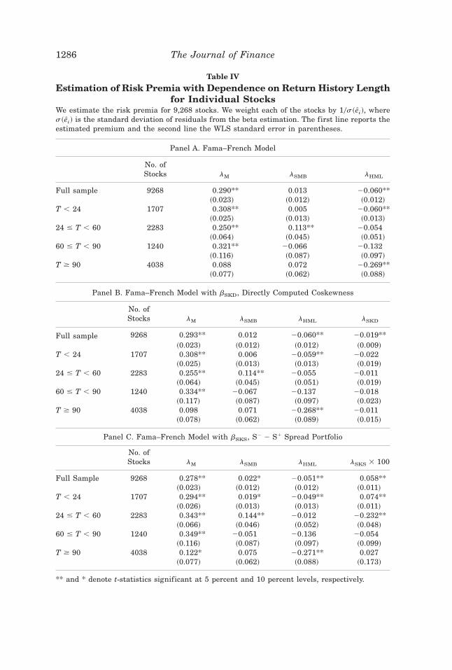
Table IV

Estimation of Risk Premia with Dependence on Return History Lengthfor Individual Stocks

We estimate the risk premia for 9,268 stocks. We weight each of the stocks by 10s~ [ei!, wheres~ [ei! is the standard deviation of residuals from the beta estimation. The first line reports theestimated premium and the second line the WLS standard error in parentheses.

Panel A. Fama–French Model

No. ofStocks lM lSMB lHML

Full sample 9268 0.290** 0.013 20.060**~0.023! ~0.012! ~0.012!

T , 24 1707 0.308** 0.005 20.060**~0.025! ~0.013! ~0.013!

24 # T , 60 2283 0.250** 0.113** 20.054~0.064! ~0.045! ~0.051!

60 # T , 90 1240 0.321** 20.066 20.132~0.116! ~0.087! ~0.097!

T $ 90 4038 0.088 0.072 20.269**~0.077! ~0.062! ~0.088!

Panel B. Fama–French Model with bSKD, Directly Computed Coskewness

No. ofStocks lM lSMB lHML lSKD

Full sample 9268 0.293** 0.012 20.060** 20.019**~0.023! ~0.012! ~0.012! ~0.009!

T , 24 1707 0.308** 0.006 20.059** 20.022~0.025! ~0.013! ~0.013! ~0.019!

24 # T , 60 2283 0.255** 0.114** 20.055 20.011~0.064! ~0.045! ~0.051! ~0.019!

60 # T , 90 1240 0.334** 20.067 20.137 20.018~0.117! ~0.087! ~0.097! ~0.023!

T $ 90 4038 0.098 0.071 20.268** 20.011~0.078! ~0.062! ~0.089! ~0.015!

Panel C. Fama–French Model with bSKS, S2 2 S1 Spread Portfolio

No. ofStocks lM lSMB lHML lSKS 3 100

Full Sample 9268 0.278** 0.022* 20.051** 0.058**~0.023! ~0.012! ~0.012! ~0.011!

T , 24 1707 0.294** 0.019* 20.049** 0.074**~0.026! ~0.013! ~0.013! ~0.011!

24 # T , 60 2283 0.343** 0.144** 20.012 20.232**~0.066! ~0.046! ~0.052! ~0.048!

60 # T , 90 1240 0.349** 20.051 20.136 20.054~0.116! ~0.087! ~0.097! ~0.099!

T $ 90 4038 0.122* 0.075 20.271** 0.027~0.077! ~0.062! ~0.088! ~0.173!

** and * denote t-statistics significant at 5 percent and 10 percent levels, respectively.


decline as more return observations become available.15 Book-to-market valuediffers substantially across return histories as well. One possible reason isthat book-to-market proxies for differences in return history lengths. This issupported by the fact that the average, log, book-to-market ratio for stockswith more than 90 months of returns is 3.85 as compared to an average, log,book-to-market ratio of 6.39 for stocks with fewer than 60 months of returns.These findings suggest that the size effect is related to how long a stock islisted. The size factor appears important only for new firms. SMB and HMLappear to be more important for firms where the number of returns avail-able to estimate the market beta is small. This may also be an IPO effect, inother words, factors other than market ~such as SMB or HML! may be moreuseful in predicting the returns on firms with a short return history.

The results show that substantial differences exist between the perfor-mance of asset pricing models in portfolios and individual equities. There-fore, to investigate the robustness of our results, we also examine a numberof portfolios of the CRSP returns formed on a variety of criteria such asbook-to-market value, return on assets, etc. These criteria are known to becorrelated with expected returns and, hence, as Berk ~2000! shows, are likelyto reject the model in question. However, we find that although the premiaestimates do vary substantially across the portfolio sorts, skewness is usu-ally significant as a factor in explaining the cross-asset variation in returns.

D. Economic Significance

Our results show that coskewness is usually statistically significant. Animportant question is whether it is economically significant. We undertaketwo additional evaluation exercises. The first focuses on the impact on themodel’s pricing errors and the second measures the expected return impliedby a change in coskewness.

Consider the root mean squared in-sample pricing error ~RMSE!. Ghysels~1998! argues that this is an important metric for model evaluation.16 Welook at each model’s RMSE relative to the CAPM’s RMSE. This exercise isrelated to Table III. With the size and book-to-market value-sorted port-folios, the addition of the SMB and HML factors reduces the base RMSE by48 percent. Adding the skewness spread, reduces the RMSE by another 10 per-cent. Similarly, for the 10 “momentum” portfolios, RMSE is reduced fromthe CAPM RMSE by 29 percent on adding SMB and HML. Inclusion of cosk-ewness reduces the RMSE by a further 17 percent. When we examine theindividual stocks, the general reductions in the RMSEs are smaller ~becauseof the limited explanatory power for individual securities!. As with the port-folio results, the introduction of the SMB and HML portfolios reduces the

15 We also analyze the 4,603 stocks in COMPUSTAT over the January 1970 through Decem-ber 1993 period alone. The results are similar to those for CRSP stocks and are available fromthe authors. There is also an issue of survivorship in the comparisons between CRSP andCOMPUSTAT data, see Kothari et al. ~1995! and Breen and Korajczyk ~1993!.

16 Chen, Kan, and Zhang ~1997! provide a critique of using t-ratios in model evaluation.


RMSE from the base case and there is a further reduction when the skew-ness spread ~or the direct estimate of skewness! is added. However, in con-trast to the portfolio results, introducing skewness alone as a second factorreduces the RMSE more than adding both HML and SMB as second andthird factors. The RMSE analysis is suggestive that skewness plays an im-portant role.

A second exercise is to assess the impact of ignoring skewness on expectedreturns. We calculate the cross-sectional distribution of the skewness spreadbetas for all individual firms. If we perturb the coskewness beta by onecross-sectional standard deviation, it translates into a 2.34 percent expectedreturn on an annual basis. This assumes that all other factor loadings areheld constant. The corresponding additional returns for the same perturba-tion for size and book-to-market value are 0.62 percent and 6.01 percent,respectively.

E. Momentum Strategies and Skewness

Momentum or relative strength strategies have posed the great challengefor asset pricing models. Jegadeesh and Titman ~1993! present evidence thatthe strategy of buying winners and selling losers where the losers and win-ners are defined on the basis of past returns can produce abnormal returns.Grinblatt, Titman, and Wermers ~1995! and Carhart ~1997! provide evidencethat a large component of mutual fund abnormal returns can be generatedby the momentum strategy of buying past winners and selling past losers.We examine the various momentum strategies with the objective of under-standing how the abnormal returns from momentum strategies relate toskewness. The summary statistics on two widely used sets of momentumportfolios in Panels C and E of Table I show that, for a one-month holdingperiod, winners have substantially lower skewness than losers.

Table V presents a representative subset of the momentum portfolios forthe 1927 to 1997 period.17 Some of these results are connected to Figure 3.For every momentum definition, the skewness of the loser portfolio is higherthan that of the winner portfolio. For example in the 6,24 strategy, the loserportfolio has a mean excess return of 20.88 percent and a skewness of 0.36.The winner portfolio has a mean excess return of 7.06 percent and a skew-ness of 20.33. The higher mean strategy is associated with lower skewness.

We construct several other sets of portfolios using momentum defined forindividual stocks over five different horizons: from 36 months to two monthsbefore portfolio formation, from 24 months to two months before, from 12months to two months before, from six months to two months before, andfrom three months to two months before. We maintain a one-month gapbetween the portfolio formation and the computation of the return on the

17 Full results for every momentum definition are available at http:00www.duke.edu0charvey0Research0momentum.htm


portfolio. For each J-month momentum we rank all the stocks in the NYSE0AMEX over the periods January 1926 to December 1997 into 10 equallyweighted and value-weighted deciles and follow the post-portfolio formationreturns over six different holding periods. These six holding periods are: onemonth, three months, six months, 12 months, 24 months, and 36 months.Thus, we examine a total of 30 sets of 10-decile portfolios.

Figure 3 plots the trade-off between mean and skewness of returns for thelosers and winners for several sets of momentum strategies over the periodJanuary 1927 to December 1997. The height of the line along the Y-axis isthe mean annualized return from the strategy and the length of the linealong the X-axis indicates the difference in skewness between the losers and

Table V

Summary Statistics on Momentum StrategiesWe form equally weighted portfolios of U.S. NYSE0AMEX and Nasdaq equities using severaldefinitions of momentum that rely on past returns. The past returns are measured over 36months to two months before portfolio formation. We maintain a one-month gap between port-folio formation and computation of return on the portfolio. For each J month momentum werank all the stocks in NYSE0Amex over the periods January 1927 to December 1997 into 10equally weighted deciles and follow the post-portfolio formation returns over six different hold-ing periods. These six holding periods are: one month, three months, six months, 12 months,24 months, and 36 months. This table presents average excess return, volatility, skewness, andkurtosis for the loser portfolio ~first decile! and winner portfolio ~tenth decile! for a represen-tative subset of these momentum strategies.

HoldingPeriod No. Momentum

DecileReturn Average Volatility Skewness Kurtosis

1 6 1 2.47 34.43 2.60 19.621 6 10 20.26 29.26 1.05 8.493 6 1 25.09 20.91 1.50 12.673 6 10 6.25 18.57 0.50 3.841 12 1 2.47 35.81 2.45 18.541 12 10 23.64 27.83 0.67 6.743 12 1 26.38 21.45 1.30 10.553 12 10 10.40 18.00 0.71 6.256 12 1 26.06 14.28 0.07 1.936 12 10 6.48 12.94 0.13 2.371 24 1 12.55 39.85 3.25 25.361 24 10 19.81 24.84 20.22 3.243 24 1 20.05 23.01 1.72 12.343 24 10 10.04 15.91 20.24 2.476 24 1 20.88 14.91 0.36 2.496 24 10 7.06 11.58 20.33 1.47

12 24 1 0.86 10.21 0.14 2.1712 24 10 4.11 8.67 20.63 0.72


winners as a result of the strategy. The negative slope of the line indicatesthat in a momentum-based trading strategy, buying the winner and sellingthe loser requires acceptance of substantial negative skewness.18

Next we examine how moments of the momentum-sorted deciles vary acrossthe portfolios. We first test using all six holding periods across the fivedefinitions of momentum jointly over the period January 1926 to December1997. Using a multivariate t-test using the Bonferroni correction for depen-dence across deciles, we reject the hypothesis that the mean returns areequal across the deciles with a p-value of 0.001. Over this period, the aver-age excess return for the loser decile is 1.15 percent per year in contrast tothe average return in winner decile of 6.77 percent per year. When we ex-clude holding periods greater than 12 months, the respective average re-turns are 0.29 percent and 8.50 percent a year. Consistent with the resultsin Jegadeesh and Titman ~1993!, we find that the betas and volatilitiesof the momentum deciles are not significantly different from each other.~ p-values are 1.000 for betas and 0.334 for volatilities.!19 Similar to Jegadeeshand Titman, we also find that, for most of the deciles, the strategy of selling

18 We have also examined a sample excluding the crash of 1929 and found similar results.19 Without a Bonferroni correction, the p-value is 0.083 for the equality for volatilities.

Figure 3. Trade-off between mean and skewness of returns in momentum tradingstrategies. This graph plots the trade-off in mean and skewness of annualized returns forseveral sets of momentum trading strategies using returns over the period January 1927 toDecember 1997. For each strategy M indicates the period over which the momentum is com-puted and H indicates the number of months over which the portfolio is held. The height of theline along the Y-axis indicates the mean annual return from the strategy and the length alongthe X-axis indicates the change in skewness.


the loser and buying the winner has a negative beta. However, when we testif skewness is identical across the deciles, we reject with a p-value of 0.001.The average skewness for the losers is 0.494, whereas the average skewnessfor winners is 20.380. The results for kurtosis also reject the hypothesisthat kurtosis is identical across the deciles.

We also examine various subsamples. For the period January 1951 to De-cember 1997, we find that the average returns on the loser and winner dec-iles are 0.47 percent and 5.26 percent a year. As before, we fail to reject thehypothesis that volatilities are identical across the deciles. The average skew-ness for the loser decile is 0.031 and for the winner decile is 20.673, and thehypothesis that skewness is identical across the deciles is very strongly re-jected. In contrast to the longer sample, for this subsample we fail to rejectthe hypothesis that average kurtosis across the deciles is identical.

The final exercise is to understand the fundamentals behind momentum.We select the second quarter of 1989 and 1993 and analyze the fundamentalcharacteristics of stocks sorted on 12-month momentum in these periods. Wecompare these characteristics to those of stocks sorted on coskewness in thesame periods. We choose 1989 and 1993 because they bracket the recessionof 1990. We select only stocks that have remained in the same decile duringthe second quarter.

The results are presented in Table VI. For coskewness, our analysis sug-gests that characteristics of coskewed firms vary over time since 1989 and1993 look different. In general, the most negatively coskewed and most pos-itively coskewed firms are different from stocks in the middle. In both years,earnings growth for positively coskewed firms is substantially higher thanfor negatively coskewed firms. In 1993, positively coskewed firms are alsolarger in size than negatively coskewed firms and possess substantially higherP0E ratios. For momentum-sorted portfolios, both the “losers” and the “win-ners” are smaller than the middle deciles. Additionally, the “losers” havenegative return on assets and much lower ratings on their debt.

Some caution should be used in interpreting these results. The regressionsin Table IV indicate that coskewness is even more important for stocks withshort histories and less important for stocks with longer histories. Never-theless, these exercises suggest that skewness plays an important economicrole.

F. Extensions

The model and results presented in this paper have several interestingextensions. For both U.S. and world portfolios, the unconditional skewnessis negative over the periods considered. Since the price of skewness shouldbe negative, the implied risk premium from skewness should be positive.Hence, the implied market risk premium from variance and skewness shouldbe higher than that from variance alone for a large number of the periods.This has the potential of helping to explain the equity market risk premiumpuzzle—the fact that unconditionally the equity market risk premium is


Tab

leV

I

Fu

nd

amen

tal

Ch

arac

teri

stic

sof

Com

pan

ies

inM

omen

tum

an

dC

osk

ewn

ess

Dec

iles

We

form

valu

e-w

eigh

ted

port

foli

osof

U.S

.N

YS

E0A

ME

Xan

dN

asda

qeq

uit

ies

inth

ese

con

dqu

arte

rsof

1989

and

1993

base

don

cosk

ewn

ess

and

t2

12to

t2

2m

omen

tum

.W

eth

ense

lect

stoc

ksth

atar

ein

the

sam

ede

cile

inal

lth

ree

mon

ths

ofth

equ

arte

r.N

ext,

we

use

CO

MP

US

TA

Tto

com

pute

the

mea

nfu

nda

men

tal

char

acte

rist

ics

ofth

ese

stoc

ks.

All

data

exce

ptfo

rgr

owth

are

from

the

ann

ual

file

s.R

etu

rnon

asse

tsis

perc

enti

zed.

Lev

erag

eis

defi

ned

aslo

ng-

term

debt

over

com

mon

equ

ity

~wit

hth

ead

diti

onof

bala

nce

shee

tde

ferr

edta

xes

and

inve

stm

ent

tax

cred

itto

and

subt

ract

ion

ofpr

efer

red

stoc

kva

lue

from

com

mon

equ

ity.

!B

ook0

mar

ket

rati

ois

com

mon

equ

ity

over

mar

ket

capi

tali

zati

on.

Rat

ing

isba

sed

onth

e15

-poi

nt

scal

eu

sed

byS

tan

dard

&P

oor’

sw

ith

10re

pres

enti

ng

BB

B.

Hig

her

nu

mbe

rsm

ean

low

erra

tin

gs.

Mat

uri

tyis

base

don

the

S&

Pbr

eakd

own

ofde

btin

tofi

veca

tego

ries

repr

esen

tin

gh

owm

uch

debt

isdu

ein

each

year

wit

hal

lof

the

debt

due

inye

arfi

veor

late

rbe

ing

com

bin

ed.

Sal

esgr

owth

,E

PS

~pri

mar

y!gr

owth

,de

btgr

owth

,an

das

set

grow

thar

epe

rcen

tize

dlo

gari

thm

icgr

owth

sfr

omth

efi

rst

toth

ese

con

dqu

arte

r.

Year

Dec

ile

Ret

urn

onA

sset

sL

ever

age

Boo

k0M

arke

tR

atio

Rat

ing

Mat

uri

tyP0

ER

atio

Siz

e~i

nM

M!

Sal

esG

row

thE

PS

Gro

wth

Deb

tG

row

thA

sset

Gro

wth

Pan

elA

.F

un

dam

enta

lC

har

acte

rist

ics

ofC

oske

wn

ess-

Sor

ted

Dec

iles

1989

12.

772.

380.

7510

.19

2.98

19.1

813

28.2

42.

422

1.14

2.91

2.48

53.

440.

580.

7410

.62

2.79

14.3

012

26.1

96.

0212

.43

0.13

2.02

64.

060.

910.

829.

642.

8325

.69

1268

.61

4.13

8.02

3.60

1.52

104.

271.

040.

7810

.91

2.93

17.8

815

81.9

83.

6313

.06

3.55

1.32

1993

12

2.16

0.68

0.81

13.1

32.

6416

.99

345.

733.

564.

511.

594.

415

14.8

10.

760.

7110

.76

2.72

11.2

677

7.91

4.13

6.98

1.86

2.54

62

6.61

0.74

0.59

11.0

72.

561.

5489

6.91

8.02

23.

080.

175.

0810

23.

350.

920.

5911

.35

2.60

28.7

681

1.85

3.52

8.90

23.

344.

96

Pan

elB

.F

un

dam

enta

lC

har

acte

rist

ics

oft

212

tot

22

Mom

entu

m-S

orte

dD

ecil

es

1989

12

12.4

015

.90

1.12

17.4

02.

582.

0438

.63

0.70

8.40

0.60

20.

205

213

.30

0.55

0.76

11.0

02.

745.

1328

7.05

11.3

02

5.90

5.80

2.10

64.

200.

740.

889.

502.

8919

.58

349.

290.

102

6.70

0.20

0.80

109.

300.

730.

3413

.60

2.44

17.1

386

5.20

14.5

05.

202

8.80

7.30

1993

12

22.0

01.

150.

7119

.25

2.29

3.37

90.0

01.

8011

.10

8.20

2.10

50.

800.

570.

7811

.44

2.68

21.0

824

46.2

02

2.20

9.10

222

.80

6.50

66.

000.

700.

7910

.00

2.69

20.6

999

9.74

2.00

32.4

02

8.50

2.30

103.

102.

040.

6512

.56

2.66

17.3

146

6.46

12.8

09.

902

9.00

9.70


higher than what one should expect from variance alone. The model andresults of this paper may also have implications for asset allocation andportfolio analysis. Instead of analyzing portfolios in a conditional mean-variance framework, a richer conditional mean-variance-skewness frame-work may be employed. The impact of skewness on option prices is alsoanother possible extension of this paper. Finally, the asymmetric variancephenomenon ~high conditional variance when returns are negative! found inmany financial markets may also have an explanation based on conditionalskewness.

IV. Conclusions

Cross-sectional tests of the single factor asset pricing model have shownthat systematic risk as measured by the covariance ~or the beta! with themarket and other factors does not satisfactorily explain the cross-sectionalvariation in expected excess returns. We provide a possible explanation forthese failures. Our intuition is that if investors know that the asset returnshave conditional coskewness at time t, expected returns should include acomponent attributable to conditional coskewness. Our asset pricing modelformalizes this intuition by incorporating measures of conditional coskewness.

We estimate this model for several sets of equity returns, both individu-ally as well as jointly, using portfolios formed using different criteria. Ourresults show that coskewness is important. In general, we find that a modelincorporating coskewness is helpful in explaining the cross-sectional varia-tion of equity returns. Coskewness also provides us with some insights as towhy why variables such as size and book-to-market value are important inexplaining the cross-sectional variation of asset returns. We also find thatthe momentum effect is related to systematic skewness. However, given thedata limitations, measurement of ex ante skewness is difficult. Variablessuch as size and book-to-market value might capture information about exante skewness that we cannot measure from past returns alone.

REFERENCES

Amihud, Yakov, Bent J. Christensen, and Haim Mendelson, 1993, Further evidence on therisk-return relationship, Working paper, New York University.

Arrow, Kenneth J., 1964, Aspects of the theory of risk-bearing; Lectures, Helsinki, Finland.Bansal, Ravi, and S. Viswanathan, 1993, No arbitrage and arbitrage pricing, Journal of Finance

48, 1231–1262.Bawa, Vijay, and Eric Lindenberg, 1977, Capital market equilibrium in a mean-lower partial

moment framework, Journal of Financial Economics 5, 189–200.Berk, Jonathan B., 2000, Sorting out sorts, Journal of Finance 55, 407–427.Black, Fischer, 1972, Capital market equilibrium with restricted borrowing, Journal of Busi-

ness 44, 444–455.Breen, William, and Robert A. Korajczyk, 1993, On selection biases in book-to-market based

tests of asset pricing models, Working paper, Northwestern University.Brennan, Michael, 1993, Agency and asset pricing, Unpublished manuscript, UCLA and Lon-

don Business School.


Campbell, John, 1993, Intertemporal asset pricing without consumption data, American Eco-nomic Review 83, 487–511.

Carhart, Mark M., 1997, On persistence in mutual fund performance, Journal of Finance 52,57–82.

Carhart, Mark M., Robert J. Krail, Robert I. Stevens, and Kelly E. Welch, 1994, Testing theconditional CAPM, Unpublished manuscript, University of Chicago.

Chan, Louis, Yasushi Hamao, and Josef Lakonishok, 1991, Fundamentals and stock returns inJapan, Journal of Finance 46, 1739–1764.

Chen, Nai-Fu, Raymond Kan, and Chu Zhang, 1997, A critique of the use of t-ratios in modelselection, Working paper, University of California, Irvine.

Christie, Andrew A., 1982, The stochastic behavior of common stock variances: Value, leverage,and interest rate effects, Journal of Financial Economics 23, 407–432.

Cochrane, John, 1994, Discrete time empirical finance; Lecture notes, University of Chicago.Fama, Eugene, and Kenneth French, 1989, Business conditions and expected returns on stocks

and bonds, Journal of Financial Economics 59, 23–49.Fama, Eugene, and Kenneth French, 1992, The cross-section of expected stock returns, Journal

of Finance 47, 427–465.Fama, Eugene, and Kenneth French, 1995, Size and book-to-market factors in earnings and

returns, Journal of Finance 50, 131–155.Fama, Eugene, and Kenneth French, 1996, Multifactor explanations of asset pricing anomalies,

Journal of Finance 51, 55–84.Fama, Eugene, and Kenneth French, 1997, Industry costs of equity, Journal of Financial Eco-

nomics 43, 153–193.Fama, Eugene, and James MacBeth, 1973, Risk, return and equilibrium: Empirical tests, Jour-

nal of Political Economy 81, 607–636.Ferson, Wayne E., and Campbell R. Harvey, 1998, Conditioning variables and the cross-section

of stock returns, Working paper, Duke University.Friend, Irwin, and Randolph Westerfield, 1980, Co-skewness and capital asset pricing, Journal

of Finance 35, 897–914.Ghysels, Eric, 1998, On stable factor structures in the pricing of risk: Do time-varying betas

help or hurt?, Journal of Finance 53, 457–482.Gibbons, Michael, Stephen Ross, and Jay Shanken, 1989, A test of the efficiency of a given

portfolio, Econometrica 57, 1121–1152.Golec, Joseph, and Maurry Tamarkin, 1998, Bettors love skewness, not risk, at the horse track,

Journal of Political Economy 106, 205–225.Grinblatt, Mark, Sheridan Titman, and Russ Wermers, 1995, Momentum investment strat-

egies, portfolio performance, and herding: A study of mutual fund behavior, American Eco-nomic Review 85, 1088–1105.

Handa, Puneet, S. P. Kothari, and Charles Wasley, 1989, The relation between the return in-terval and betas—Implications for the size effect, Journal of Financial Economics 23, 79–100.

Hansen, Lars, and Ravi Jagannathan, 1991, Implications of security market data for models ofdynamic economies, Journal of Political Economy 99, 225–262.

Hansen, Lars, and Scott Richard, 1987, The role of conditioning information in deducing test-able restrictions implied by dynamic asset pricing models, Econometrica 55, 587–613.

Hansen, Lars, and Kenneth Singleton, 1983, Stochastic consumption, risk aversion, and thetemporal behavior of asset returns, Journal of Political Economy 91, 249–265.

Harrison, Michael, and David Kreps, 1979, Martingales and arbitrage in multi-period securi-ties markets, Journal of Economic Theory 20, 381–408.

Harvey, Campbell, and Akhtar Siddique, 1999, Autoregressive conditional skewness, Journal ofFinancial and Quantitative Analysis 34, 465–487.

Ingersoll, Jonathan, Jr. 1990, Theory of Financial Decision Making, ~Rowman and Littlefield,Totowa, New Jersey.!

Jagannathan, Ravi, and Z. Wang, 1996, The conditional CAPM and the cross-section of expectedreturns, Journal of Finance 53, 3–53.


Jegadeesh, Narasimhan, and Sheridan Titman, 1993, Returns to buying winners and sellinglosers: Implications for stock market efficiency, Journal of Finance 48, 65–91.

Kan, Raymond, and Chu Zhang, 1997, Tests of asset pricing models with useless factors, Work-ing paper, University of Toronto.

Kandel, Shmuel, and Robert Stambaugh, 1995, Bayesian inference and portfolio efficiency,Review of Financial Studies 8, 1–53.

Kim, Dongcheol, 1995, The errors in the variables problem in the cross-section of expected stockreturns, Journal of Finance 50, 1605–1634.

Kimball, Miles, 1990, Precautionary saving in the small and in the large, Econometrica 58,53–73.

Kothari, S. P., Jay Shanken, and Richard Sloan, 1995, Another look at the cross-section ofexpected stock returns, Journal of Finance 50, 185–224.

Kraus, Alan, and Robert Litzenberger, 1976, Skewness preference and the valuation of riskassets, Journal of Finance 31, 1085–1100.

Lakonishok, Josef, Andrei Shleifer, and Robert Vishny, 1994, Contrarian investment, extrapo-lation, and risk, Journal of Finance 49, 1541–1578.

Leland, Hayne, 1997, Beyond mean-variance: Performance measurement of portfolios usingoptions or dynamic strategies, Working paper, University of California, Berkeley.

Lim, Kian-Guan, 1989, A new test of the three-moment capital asset pricing model, Journal ofFinancial and Quantitative Analysis 24, 205–216.

Lintner, John, 1965, The valuation of risk assets and the selection of risky investments in stockportfolios and capital budgets, Review of Economics and Statistics 47, 13–37.

Merton, Robert, 1982, On the mathematics and economics assumptions of continuous-time mod-els, in William F. Sharpe and Cathryn M. Cootner, eds.: Financial Economics: Essays inhonor of Paul Cootner, Prentice-Hall, Englewood Cliffs, NJ.

Nelson, Daniel, 1991, Conditional heteroskedasticity in asset returns, Econometrica 59, 347–370.Nummelin, Kim, 1994, Expected asset returns and financial risks, Dissertation, Swedish School

of Economics and Business Administration ~Svenska Handelshögskolan!, Helsinki, Finland.Racine, Marie, 1995, Volatility shocks, conditional coskewness, conditional beta and asset pric-

ing, Unpublished manuscript, Wilfrid Laurier University.Roll, Richard, and Stephen Ross, 1994, On the cross-sectional relation between expected re-

turns and betas, Journal of Finance 49, 101–121.Roll, Richard, 1977, A critique of the asset pricing theory’s tests, Part I: On past and potential

testability of theory, Journal of Financial Economics 4, 129–176.Ross, Stephen, 1977, The capital asset pricing model ~CAPM!, short-sale restrictions and re-

lated issues, Journal of Finance 32, 177–183.Scholes, Myron, and Joseph Williams, 1977, Estimating betas from nonsynchronous data, Jour-

nal of Financial Economics 14, 327–348.Scott, Robert, and Philip Horvath, 1980, On the direction of preference for moments of higher

order than the variance, Journal of Finance 35, 915–919.Sears, R. Stephen, and K-C. John Wei, 1985, Asset pricing, higher moments, and the market

risk premium: A note, Journal of Finance 40, 1251–1253.Shanken, Jay, 1992, On the estimation of beta-pricing models, Review of Financial Studies 5,

1–33.Sharpe, William, 1964, Capital asset prices: A theory of market equilibrium under conditions of

risk, Journal of Finance 19, 425–442.Waldron, Paddy, 1990, Three-moment and three-fund results in portfolio theory, Working paper,

University of Pennsylvania.


1296

Documents

Conditional Skewness in Asset Pricing Testscharvey/Teaching/CDROM_BA456_200… · Conditional Skewness in Asset Pricing Tests ... tum portfolios have higher skewness ... turns more