Conditional Time Series Forecasting with Convolutional Neural

Networks

Anastasia Borovykh∗ Sander Bohte † Cornelis W. Oosterlee ‡§

This version: October 18, 2017

Abstract

We present a method for conditional time series forecasting based on the recent deep convolutional

WaveNet architecture. The proposed network contains stacks of dilated convolutions that allow it to

access a broad range of history when forecasting; multiple convolutional filters are applied in parallel

to separate time series and allow for the fast processing of data and the exploitation of the correlation

structure between the multivariate time series. The performance of the deep convolutional neural network

is analyzed on various multivariate time series and compared to that of the well-known autoregressive

model and a long-short term memory network. We show that our network is able to effectively learn

dependencies between the series without the need for long historical time series and can outperform the

baseline neural forecasting models.

Keywords: Convolutional neural network, financial time series, forecasting, deep learning, multivariate

time series

1 Introduction

Forecasting financial time series using past observations has been a topic of significant interest for obvious

reasons. It is well known that while temporal relationships in the data exist, they are difficult to analyze

and predict accurately due to the non-linear trends and noise present in the series. In developing models

for forecasting financial data it is desirable that these will be both able to learn non-linear dependencies in

the data as well as have a high noise resistance. Feedforward neural networks have been a popular way of

learning the dependencies in the data, by e.g. using multiple inputs from the past to make a prediction for

the future time step, see [3]. One downside of classical feedforward neural networks is that a large sample

size of data is required to obtain a stable forecasting result.

The main focus of this paper is on multivariate time series forecasting, specifically financial time series.

In particular, we forecast time series conditional on other, related series. Financial time series are known to

∗Dipartimento di Matematica, Universita di Bologna, Bologna, Italy. e-mail: anastasia.borovykh2@unibo.it†Centrum Wiskunde & Informatica, Amsterdam, The Netherlands. e-mail:s.m.bohte@cwi.nl‡Centrum Wiskunde & Informatica, Amsterdam, The Netherlands. e-mail: c.w.oosterlee@cwi.nl§Delft University of Technology, Delft, The Netherlands

1

arX

iv:1

703.

0469

1v3

[st

at.M

L]

16

Oct

201

7

both have a high noise component as well as to be of limited duration – even when available, the use of long

histories of stock prices can be difficult due to the changing financial environment. At the same time, many

different, but strongly correlated financial time series exist. Here, we aim to exploit multivariate forecasting

using the notion of conditioning to reduce the noisiness in short duration series. Effectively, we use multiple

financial time series as input in a neural network, thus conditioning the forecast of a time series x(t) on both

its own history as well as that of multiple other time series y1(t), y2(t), .... Training a model on multiple

stock series allows the network to exploit the correlation structure between these series so that the network

can learn the market dynamics in shorter sequences of data. Furthermore, using multiple conditional time

series as inputs can improve both the robustness and forecast quality of the model by learning long-term

temporal dependencies in between series.

A convolutional neural network (CNNs) is a type of network that has recently gained popularity due to

its success in classification problems (e.g. image recognition [11] or time series classification [15]). The CNN

consists of a sequence of convolutional layers, the output of which is connected only to local regions in the

input. This is achieved by sliding a filter, or weight matrix, over the input and at each point computing

the dot product between the two (i.e. a convolution between the input and filter). This structure allows

the model to learn filters that are able to recognize specific patterns in the input data. The authors in

[2] propose to use an autoregressive-type weighting system for forecasting financial time series, where the

weights are allowed to be data-dependent by learning them through a CNN. Besides this paper, literature

on financial time series forecasting with convolutional architectures is still scarce, as these type of networks

are much more commonly applied in classification problems. Intuitively, the idea of applying CNNs to time

series forecasting would be to learn filters that represent certain repeating patterns in the series and use

these to forecast the future values. Due to the layered structure of CNNs, they might work well on noisy

series, by discarding in each subsequent layer the noise and extracting only the meaningful patterns.

Currently, recurrent neural networks (RNNs), and in particular the long-short term memory unit (LSTM),

are the state-of-the-art in time series forecasting. The efficiency of these networks can be explained by the

recurrent connections that allow the network to access the entire history of previous time series values.

Alternatively one might employ a convolutional neural network with multiple layers of dilated convolutions.

The dilated convolutions, in which the filter is applied by skipping certain elements in the input, allow for

the receptive field of the network to grow exponentially, hereby allowing the network to, similar to the RNN,

access a broad range of history. The advantage of the CNN over the recurrent-type network is that due to the

convolutional structure of the network, the number of trainable weights is small, resulting in a much more

efficient training and predicting. Motivated by [14] in which the authors compare the performance of the

PixelCNN to the PixelRNN, a network used for image generation, in this paper, we aim to investigate the

performance of the convolutional neural network compared to that of autoregressive and recurrent models

on forecasting noisy, financial time series.

The CNN we employ is a network inspired by the convolutional WaveNet model from [13] first developed

for audio forecasting. The network focusses on learning long-term relationships in and between multivariate,

noisy time series. It makes use of the dilated convolutions applied with parametrized skip connections [7]

from the input time series as well as the time series we condition on, in this way learning long- and short-

2

term interdependencies in an efficient manner. Knowing the strong performance of CNNs on classification

problems we show that they can be applied successfully to forecasting financial time series of limited length.

By comparing the performance of the WaveNet model to that of an LSTM, the current state-of-the-art

in forecasting, and an autoregressive model popular in econometrics, we show that our model is a time-

efficient and easy to implement alternative to recurrent-type networks and performs better than a linear

autoregressive model. Finally, we show that the efficient way of conditioning in the WaveNet model enables

one to extract temporal relationships in between time series improving the forecast, while at the same time

limiting the requirement for a long historical price series and reducing the noise, since it allows one to exploit

the correlations in between related time series.

2 The model

In this section we start with a review of neural networks and convolutional neural networks. Then we

introduce the particular convolutional network structure that will be used for time series forecasting.

2.1 Background

2.1.1 Feedforward neural networks

A basic feedforward neural network consists of L layers with Ml hidden nodes in each layer l = 1, ..., L.

Suppose we are given as input x(1), ..., x(t) and we want to use the multi-layer neural network to output the

forecasted value at the next time step x(t+ 1). In the first layer we construct M1 linear combinations of the

input variables in the form

a1(i) =

t∑j=1

w1(i, j)x(j) + b1(i), for i = 1, ...,M1,

where w1 ∈ RM1×t are referred to as the weights and b1 ∈ RM1 as the biases. Each of the outputs a1(i),

i = 1, ...,M1 are then transformed using a differentiable, nonlinear activation function h(·) to give

f1(i) = h(a1(i)), for i = 1, ...,M1.

The nonlinear function enables the model to learn nonlinear relations between the data points. In every

subsequent layer l = 2, ..., L − 1, the outputs from the previous layer f l−1 are again linearly combined and

passed through the nonlinearity

f l(i) = h

Ml−1∑j=0

wl(i, j)f l−1(j) + bl(j)

, for i = 1, ...,M1,

with wl ∈ RMl×Ml−1 and bl ∈ RMl . In the final layer l = L of the neural network the forecasted value x(t+1)

is computed using

x(t+ 1) = h

ML−1∑j=0

wL(j)fL−1(j) + bL

,

3

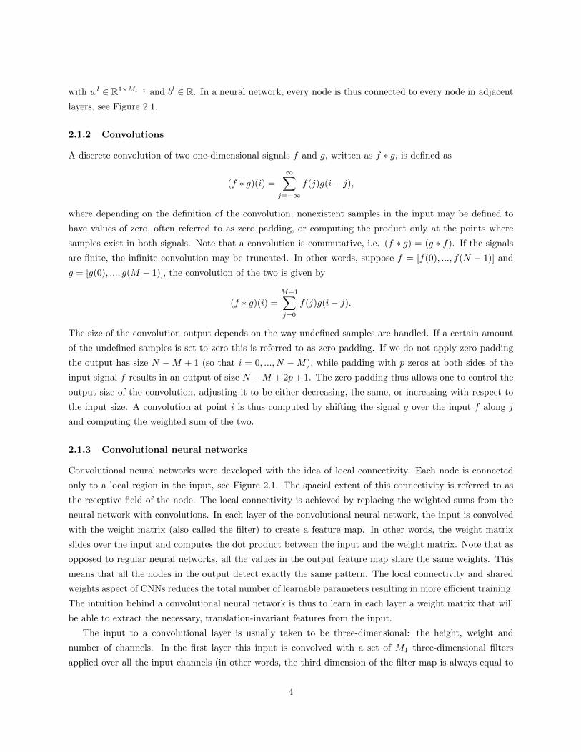
with wl ∈ R1×Ml−1 and bl ∈ R. In a neural network, every node is thus connected to every node in adjacent

layers, see Figure 2.1.

2.1.2 Convolutions

A discrete convolution of two one-dimensional signals f and g, written as f ∗ g, is defined as

(f ∗ g)(i) =

∞∑j=−∞

f(j)g(i− j),

where depending on the definition of the convolution, nonexistent samples in the input may be defined to

have values of zero, often referred to as zero padding, or computing the product only at the points where

samples exist in both signals. Note that a convolution is commutative, i.e. (f ∗ g) = (g ∗ f). If the signals

are finite, the infinite convolution may be truncated. In other words, suppose f = [f(0), ..., f(N − 1)] and

g = [g(0), ..., g(M − 1)], the convolution of the two is given by

(f ∗ g)(i) =

M−1∑j=0

f(j)g(i− j).

The size of the convolution output depends on the way undefined samples are handled. If a certain amount

of the undefined samples is set to zero this is referred to as zero padding. If we do not apply zero padding

the output has size N −M + 1 (so that i = 0, ..., N −M), while padding with p zeros at both sides of the

input signal f results in an output of size N −M + 2p+ 1. The zero padding thus allows one to control the

output size of the convolution, adjusting it to be either decreasing, the same, or increasing with respect to

the input size. A convolution at point i is thus computed by shifting the signal g over the input f along j

and computing the weighted sum of the two.

2.1.3 Convolutional neural networks

Convolutional neural networks were developed with the idea of local connectivity. Each node is connected

only to a local region in the input, see Figure 2.1. The spacial extent of this connectivity is referred to as

the receptive field of the node. The local connectivity is achieved by replacing the weighted sums from the

neural network with convolutions. In each layer of the convolutional neural network, the input is convolved

with the weight matrix (also called the filter) to create a feature map. In other words, the weight matrix

slides over the input and computes the dot product between the input and the weight matrix. Note that as

opposed to regular neural networks, all the values in the output feature map share the same weights. This

means that all the nodes in the output detect exactly the same pattern. The local connectivity and shared

weights aspect of CNNs reduces the total number of learnable parameters resulting in more efficient training.

The intuition behind a convolutional neural network is thus to learn in each layer a weight matrix that will

be able to extract the necessary, translation-invariant features from the input.

The input to a convolutional layer is usually taken to be three-dimensional: the height, weight and

number of channels. In the first layer this input is convolved with a set of M1 three-dimensional filters

applied over all the input channels (in other words, the third dimension of the filter map is always equal to

4

the number of channels in the input) to create the feature output map. Consider now a one-dimensional

input x = (xt)N−1t=0 of size N with no zero padding. The output feature map from the first layer is then given

by convolving each filter w1h for h = 1, ...,M1 with the input:

a1(i, h) = (w1h ∗ x)(i) =

∞∑j=−∞

w1h(j)x(i− j),

where w1h ∈ R1×k×1 and a1 ∈ R1×N−k+1×M1 . Note that since the number of input channels in this case is

one, the weight matrix also has only one channel. Similar to the feedforward neural network, this output is

then passed through the non-linearity h(·) to give f1 = h(a1).

In each subsequent layer l = 2, ..., L the input feature map, f l−1 ∈ R1×Nl−1×Ml−1 , where 1×Nl−1×Ml−1

is the size of the output filter map from the previous convolution with Nl−1 = Nl−2 − k + 1, is convolved

with a set of Ml filters wlh ∈ R1×k×Ml−1 , h = 1, ...,Ml, to create a feature map al ∈ R1×Nl×Ml :

al(i, h) = (wlh ∗ f l−1)(i) =

∞∑j=−∞

Ml−1∑m=1

wlh(j,m)f l−1(i− j,m).

The output of this is then passed through the non-linearity to give f l = h(al). The filter size parameter k

thus controls the receptive field of each output node. Without zero padding, in every layer the convolution

output has width Nl = Nl−1 − k + 1 for l = 1, .., L. Since all the elements in the feature map share the

same weights this allows for features to be detected in a time-invariant manner, while at the same time it

reduces the number of trainable parameters. The output of the network after L convolutional layers will

thus be the matrix fL, the size of which depends on the filter size and number of filters used in the final

layer. Depending on what we want our model to learn, the weights in the model are trained to minimize the

error between the output from the network fL and the true output we are interested in.

Figure 2.1: A feedforward neural network with three layers (L) vs. a convolutional neural network with two

layers and filter size 1 × 2, so that the receptive field of each node consists of two input neurons from the

previous layer and weights are shared across the layers, indicated by the identical colors (R).

5

2.2 Structure

Consider a one-dimensional time series x = (xt)N−1t=0 . Given a model with parameter values θ, the task for

a predictor is to output the next value x(t+ 1) conditional on the series’ history, x(0), ..., x(t). This can be

done by maximizing the likelihood function

p(x|θ) =

N−1∏t=0

p(x(t+ 1)|x(0), ..., x(t), θ).

To learn this likelihood function, we present a convolutional neural network in the form of the WaveNet

architecture [13] augmented with a number of recent architectural improvements for neural networks such

that the architecture can be applied successfully to time series prediction.

Time series often display long-term correlations, so to enable the network to learn these long-term depen-

dencies we use stacked layers of dilated convolutions. As introduced in [16], a dilated convolution outputs a

stack of Ml feature maps given by

(wlh ∗d f l−1)(i) =

∞∑j=−∞

Ml−1∑m=1

wlh(j,m)f l−1(i− d · j,m),

where d is the dilation factor and Ml the number of channels. In other words, in a dilated convolution the

filter is applied to every dth element in the input vector, allowing the model to efficiently learn connections

between far-apart data points. We use an architecture similar to [16] and [13] with L layers of dilated

convolutions l = 1, ..., L and with the dilations increasing by a factor of two: d ∈ [20, 21, ..., 2L−1]. The filters

w are chosen to be of size 1×k := 1×2. An example of a three-layer dilated convolutional network is shown

in Figure 2.2. Using the dilated convolutions instead of regular ones allows the output y to be influenced

by more nodes in the input. The input of the network is given by the time series x = (xt)N−1t=0 . In each

subsequent layer we apply the dilated convolution, followed by a non-linearity, giving the output feature

maps f l, l = 1, ..., L. These L layers of dilated convolutions are then followed by a 1× 1 convolution which

reduces the number of channels back to one, so that the model outputs a one-dimensional vector. Since we

are interested in forecasting the subsequent values of the time series, we will train the model so that this

output is the forecasted time series x = (xt)N−1t=0 .

The receptive field of each neuron was defined as the set of elements in its input that modifies the output

value of that neuron. Now, we define the receptive field r of the model to be the number of neurons in the

input in the first layer, i.e. the time series, that can modify the output in the final layer, i.e. the forecasted

time series. This then depends on the number of layers L and the filter size k, and is given by

r := 2L−1k.

In Figure 2.2, the receptive field is given by r = 8, one output value is influenced by eight input neurons.

As we already mentioned, sometimes it is convenient to pad the input with zeros around the border. The

size of this zero-padding then controls the size of the output. In our case, to not violate the adaptability

constraint on x, we want to make sure that the receptive field of the network when predicting x(t + 1)

contains only x(0), ..., x(t). To do this we use causal convolutions, where the word causal indicates that the

6

Figure 2.2: A dilated convolutional neural network with three layers.

convolution output should not depend on future inputs. In time series this is equivalent to padding the input

with a vector of zeros of the size of the receptive field, so that the input is given by

[0, ..., 0, x(0), ..., x(N − 1)] ∈ RN+r,

and the output of the L-layer Wavenet is

[x(0), ..., x(N)] ∈ RN+1.

At training time the prediction of x(1), ..., x(N) is thus computed by convolving the input with the kernels

in each layer l = 1, ..., L, followed by the 1 × 1 convolution. At testing time a one-step ahead prediction

x(t + 1) for (t + 1) ≥ r is given by inputting [x(t + 1 − r), ..., x(t)] in the trained model. An n-step ahead

forecast is made sequentially by feeding each prediction back into the network at the next time step, e.g. a

two-step ahead out-of-sample forecast x(t+ 2) is made using [x(t+ 2− r), ..., x(t+ 1)].

The idea of the network is thus to use the capabilities of convolutional neural networks as autoregressive

forecasting models. In a simple autoregressive model of order p the forecasted value for x(t+ 1) is given by

x(t+ 1) =∑p

i=1 αixt−i + ε(t), where αi, i = 1, ..., p are learnable weights and ε(t) is white noise. With the

WaveNet model as defined above, the forecasted conditional expectation for every t ∈ {0, ..., N} is

E[x(t+ 1)|x(t), ..., x(t− r)] = β1(x(t− r)) + ...+ βr(x(t)),

where the functions βi, i = 1, ..., r are data-dependent and optimized through the convolutional network.

We remark that even though the weights depend on the underlying data, due to the convolutional structure

of the network, the weights are shared across the outputted filter map resulting in a weight matrix that is

translation-invariant.

Objective function. The network weights, the filters wlh, are trained to minimize the mean absolute error

(MAE); to avoid overfitting, i.e. too large weights, we use L2 regularization with regularization term γ, so

that the cost function is given by

E(w) =1

N

N−1∑t=0

|x(t+ 1)− x(t+ 1)|+ γ

2

L∑l=0

Ml+1∑h=1

(wlh)2, (1)

7

where x(t + 1) denotes the forecast of x(t + 1) using x(0), ..., x(t). Minimizing E(w) results in a choice of

weights that make a tradeoff between fitting the training data and being small. Too large weights often

result in the network being overfitted on the training data, so the L2 regularization, by forcing the weights

to not become too big, enables the model to generalize better on unseen data.

Remark 1 (Relation to the Bayesian framework). In a Bayesian framework minimizing this cost function

is equivalent to maximizing the posterior distribution under a Laplace distributed likelihood function centered

at the value outputted by the model x(t+ 1) with a fixed scale parameter β = 12 ,

p(x(t+ 1)|x(0), ..., x(t), θ) ∼ Laplace(x(t+ 1), β),

and with a Gaussian prior on the model parameters.

The output is obtained by running a forward pass through the network with the optimal weights being

a point estimate from the posterior distribution. Since the MAE is a scale-dependent accuracy measure one

should normalize the input data to make the error comparable for different time series.

Weight optimization. The aim of training the model is to find the weights that minimize the cost function

in (1). A standard weight optimization is based on gradient descent in which one incrementally updates the

weights based on the gradient of the error function,

wlh(τ + 1) = wl

h(τ)− η∇E(w(τ)), (2)

for τ = 1, ..., T , where T is the number of training iterations and η is the learning rate. Each iteration τ thus

consists of a forward run in which one computes the forecasted vector x and the corresponding error E(w(τ)),

and a backward pass in which the gradient vector ∇E(w(τ)), the derivatives with respect to each weight

wlh, is computed and the weights are updated according to (2). The gradient vector is computed through

backpropagation, which amounts to applying the chain rule iteratively from the error function computed in

the final layer until the gradient with respect to the required layer weight wlh is obtained:

∂E(w(τ))

∂wlh(j,m)

=

Nl∑i=1

∂E(w(τ))

∂f l(i, h)

∂f l(i, h)

∂al(i, h)

∂al(i,m)

∂wlh(j,m)

,

where we sum over all the nodes in which the weight of interest occurs. The number of training iterations

T is chosen so as to achieve convergence in the error. Here we employ a slightly modified weight update by

using the Adam gradient descent [10]. This method computes adaptive learning rates for each parameter by

keeping an exponentially decaying average of past gradients and squared gradients and use these to update

the parameters. The adaptive learning rate allows the gradient descent to find the minimum more accurately.

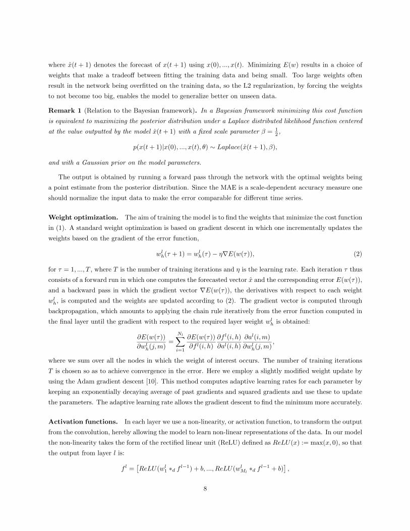
Activation functions. In each layer we use a non-linearity, or activation function, to transform the output

from the convolution, hereby allowing the model to learn non-linear representations of the data. In our model

the non-linearity takes the form of the rectified linear unit (ReLU) defined as ReLU(x) := max(x, 0), so that

the output from layer l is:

f l =[ReLU(wl

1 ∗d f l−1) + b, ..., ReLU(wlMl∗d f l−1 + b)

],

8

where b ∈ R denotes the bias that shifts the input to the nonlinearity, ∗d denotes as usual the convolution

with dilation d and f l ∈ R1×Nl×Ml+1 denotes the output of the convolution with filters whl , h = 1, ...,Ml in

layer l. Unlike the gated activation function used in [13] for audio generation, here we propose to use the

ReLU as it was found to be most efficient when applied to the forecasting of the non-stationary, noisy time

series. The final layer, l = L, has a linear activation function, which followed by the 1×1 convolution then

outputs the forecasted value of the time series x = [x(0), ..., x(N)].

When training a deep neural network, one of the problems keeping the network from learning the optimal

weights is that of the vanishing/exploding gradient [1][5]. As backpropagation computes the gradients by the

chain rule, when the derivative of the activation function takes on either small or large values, multiplication

of these numbers can result in the gradients for the weights in the initial layers to vanish or explode,

respectively. This results in either the weights being updated too slowly due to the too small gradient, or

not being able to converge to the minimum due to gradient descent step being too large. One solution to

this problem is to initialize the weights of the convolutional layers in such a way that neither in the forward

nor in the backward propagation of the network the weights reduce or magnify the magnitudes of the input

signal and gradients, respectively. A proper initialization of the weights would keep the signal and gradients

in a reasonable range of values throughout the layers so that no information will be lost while training the

network. As derived in [6], to ensure that the variance of the input is similar to the variance of the output,

a sufficient condition is

1

2zVar[wl

h] = 1, for h = 1, ...,Ml+1,∀l,

which leads to a zero-mean Gaussian distribution whose standard deviation is√

2/z, where z is the total

number of trainable parameters in the layer. In other words, the weights of the ReLU units are initialized

(for τ = 0) as

wlh ∼ N

(0,

√2

z

),

with z = Ml · 1 · k, the number of filters in layer l times the filter size 1× k.

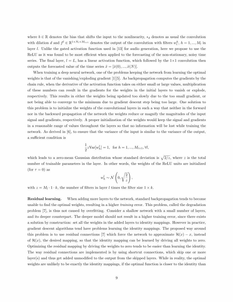
Residual learning. When adding more layers to the network, standard backpropagation tends to become

unable to find the optimal weights, resulting in a higher training error. This problem, called the degradation

problem [7], is thus not caused by overfitting. Consider a shallow network with a small number of layers,

and its deeper counterpart. The deeper model should not result in a higher training error, since there exists

a solution by construction: set all the weights in the added layers to identity mappings. However in practice,

gradient descent algorithms tend have problems learning the identity mappings. The proposed way around

this problem is to use residual connections [7] which force the network to approximate H(x) − x, instead

of H(x), the desired mapping, so that the identity mapping can be learned by driving all weights to zero.

Optimizing the residual mapping by driving the weights to zero tends to be easier than learning the identity.

The way residual connections are implemented is by using shortcut connections, which skip one or more

layer(s) and thus get added unmodified to the output from the skipped layers. While in reality, the optimal

weights are unlikely to be exactly the identity mappings, if the optimal function is closer to the identity than

9

a zero mapping, the proposed residual connections will still aid the network in learning the better optimal

weights.

Similar to [13], in our network, we add a residual connection after each dilated convolution from the input

to the convolution to the output. In the case of Ml > 1 the output from the non-linearity is passed through

a 1×1 convolution prior to adding the residual connection. This is done to make sure that the residual

connection and the output from the dilated convolution both have the same number of channels. This allows

us to stack multiple layers, while retaining the ability of the network to correctly map dependencies learned

in the initial layers.

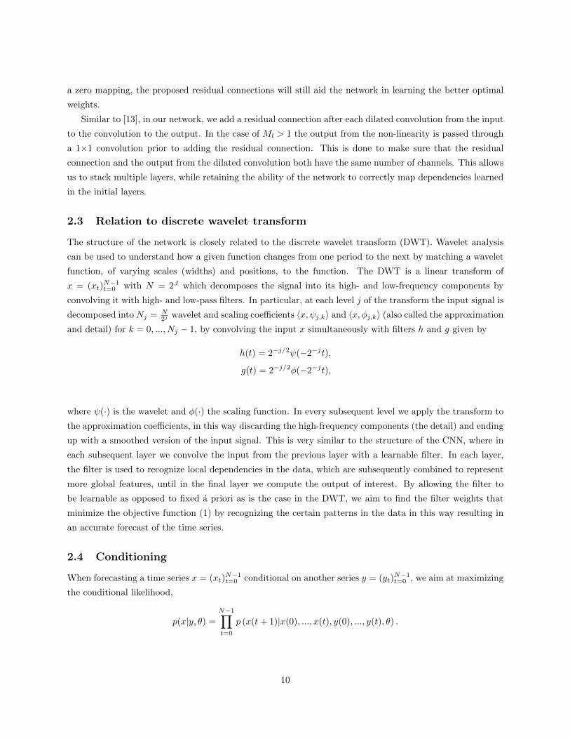
2.3 Relation to discrete wavelet transform

The structure of the network is closely related to the discrete wavelet transform (DWT). Wavelet analysis

can be used to understand how a given function changes from one period to the next by matching a wavelet

function, of varying scales (widths) and positions, to the function. The DWT is a linear transform of

x = (xt)N−1t=0 with N = 2J which decomposes the signal into its high- and low-frequency components by

convolving it with high- and low-pass filters. In particular, at each level j of the transform the input signal is

decomposed into Nj = N2j wavelet and scaling coefficients 〈x, ψj,k〉 and 〈x, φj,k〉 (also called the approximation

and detail) for k = 0, ..., Nj − 1, by convolving the input x simultaneously with filters h and g given by

h(t) = 2−j/2ψ(−2−jt),

g(t) = 2−j/2φ(−2−jt),

where ψ(·) is the wavelet and φ(·) the scaling function. In every subsequent level we apply the transform to

the approximation coefficients, in this way discarding the high-frequency components (the detail) and ending

up with a smoothed version of the input signal. This is very similar to the structure of the CNN, where in

each subsequent layer we convolve the input from the previous layer with a learnable filter. In each layer,

the filter is used to recognize local dependencies in the data, which are subsequently combined to represent

more global features, until in the final layer we compute the output of interest. By allowing the filter to

be learnable as opposed to fixed a priori as is the case in the DWT, we aim to find the filter weights that

minimize the objective function (1) by recognizing the certain patterns in the data in this way resulting in

an accurate forecast of the time series.

2.4 Conditioning

When forecasting a time series x = (xt)N−1t=0 conditional on another series y = (yt)

N−1t=0 , we aim at maximizing

the conditional likelihood,

p(x|y, θ) =

N−1∏t=0

p (x(t+ 1)|x(0), ..., x(t), y(0), ..., y(t), θ) .

10

The conditioning on the time series y is done by computing the activation function of the convolution with

filters w1h and v1h in first layer as

ReLU(w1h ∗d x+ b) +ReLU(v1h ∗d y + b),

for each of the filters h = 1, ...,M1. When predicting x(t+ 1) the receptive field of the network must contain

only x(0), ..., x(t) and y(0), ..., y(t). Therefore, similar to the input, to preserve causality the condition is

appended with a vector of zeros the size of the receptive field. In [13] the authors propose to take v1h as

a 1 × 1 filter. Given the short input window, this type of conditioning is not always able to capture all

dependencies between the time series. Therefore, we use a 1 × k convolution, increasing the probability of

the correct dependencies being learned with fewer layers. The receptive field of the network thus contains

2L−1k elements of both the input and the condition(s).

Instead of the residual connection in the first layer, we add skip connections parametrized by 1×1 convolu-

tions from both the input as well as the condition to the result of the dilated convolution. The conditioning

can easily be extended to a multivariate M × N time series by using M dilated convolutions from each

separate condition and adding them to the convolution with the input. The parametrization of the skip con-

nections makes sure that our model is able to correctly extract the necessary relations between the forecast

and both the input and condition(s). Specifically, if a particular condition does not improve the forecast, the

model can simply learn to discard this condition by setting the weights in the parametrized skip connection

(i.e. in the 1×1 convolution) to zero. This enables the conditioning to boost predictions in a discriminative

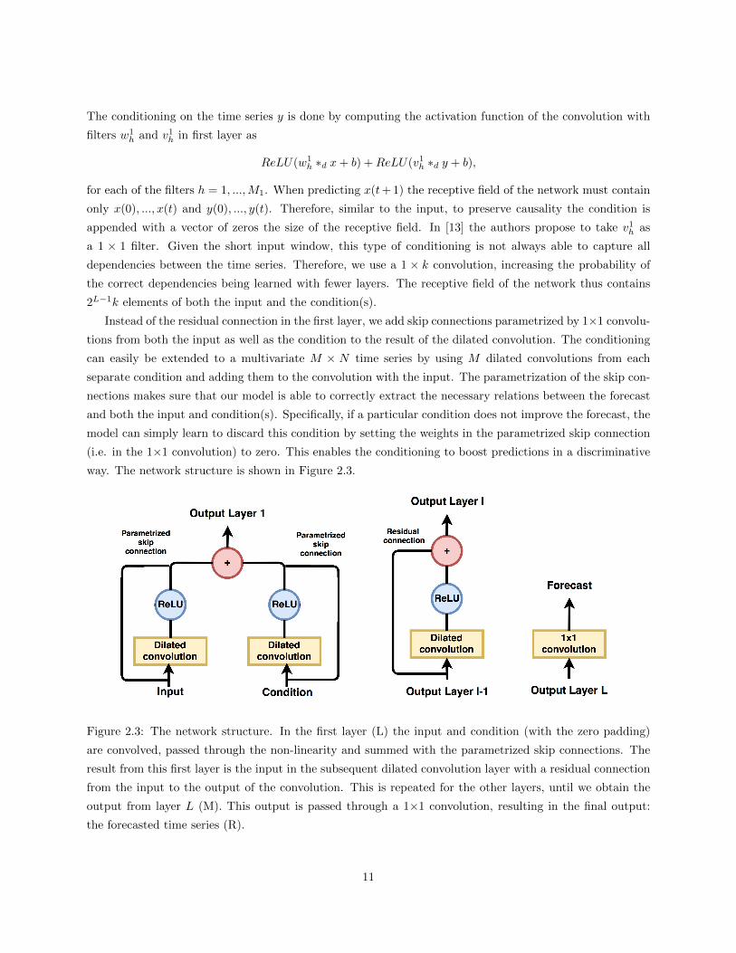
way. The network structure is shown in Figure 2.3.

Figure 2.3: The network structure. In the first layer (L) the input and condition (with the zero padding)

are convolved, passed through the non-linearity and summed with the parametrized skip connections. The

result from this first layer is the input in the subsequent dilated convolution layer with a residual connection

from the input to the output of the convolution. This is repeated for the other layers, until we obtain the

output from layer L (M). This output is passed through a 1×1 convolution, resulting in the final output:

the forecasted time series (R).

11

3 Experiments

Here, we evaluate the performance of the proposed Wavenet architecture versus current state-of-the-art

models (RNNs and autoregressive models) when applied to learning dependencies in chaotic, non-linear

time series. The parameters in the model, unless otherwise mentioned, are set to k = 2, L = 4, Ml = 1,

l = 0, ..., L − 1, the Adam learning rate is set to 0.001 and the number of training iterations is 20000. The

regularization rate is chosen to be 0.001. We train networks with different random seeds, discard any network

which underperforms already on the training set and report the average results on the test set over three

selected networks.

3.1 An artificial example

In order to show the ability of the model to learn both linear and non-linear dependencies in and between

time series, we train and test the model on the chaotic Lorenz system. The Lorenz map is defined as the

solution (X,Y, Z) to a system of ordinary differential equations (ODEs) given by

X = σ(Y −X)

Y = X(ρ− Z)− Y

Z = XY − βY,

with initial values (X0, Y0, Z0). We present in Table 3.1 the one-step ahead forecasting results for each of the

three coordinates (X,Y, Z) with the unconditional WaveNet (uWN) and the conditional Wavenet (cWN).

In the cWN the forecast of e.g. Xt contains Xt−1, ..., Xt−1−r, Yt−1, ..., Yt−1−r and Zt−1, ..., Zt−1−r. We

use a training time series of length 1000, i.e. (Xt)1000t=1 , (Yt)

1000t=1 and (Zt)

1000t=1 . Then we perform a one-step

ahead forecast of Xt, Yt and Zt for t = 1000, ..., 1500, and compare the forecasted series Xt, Yt and Zt to

the true series. The RMSE is computed over this test set. Comparing the results of the uWN with the

RMSE benchmark of 0.00675 from [9] obtained with an Augmented LSTM, we conclude that the network

is well-capable of extracting both linear and non-linear relationships in and between time series. At the

same time, conditioning on other related time series reduces the standard deviation as once can see from the

smaller standard deviation in the RMSE of the cWN compared to the uWN.

Coordinate RMSE uWN RMSE cWN

X 0.00577 (0.00242) 0.00174 (0.00133)

Y 0.00864 (0.00487) 0.00583 (0.00350)

Z 0.00496 (0.00363) 0.00536 (0.00158)

Table 3.1: RMSE (mean (standard deviation)) for the one-step ahead forecast of the Lorenz map with

(X0, Y0, Z0) = (0, 1, 1.05), σ = 10, ρ− 28 and β = 8/3. The cWN results for each coordinate are conditioned

on the other two in the system. The current benchmark RMSE is 0.00675 from [9].

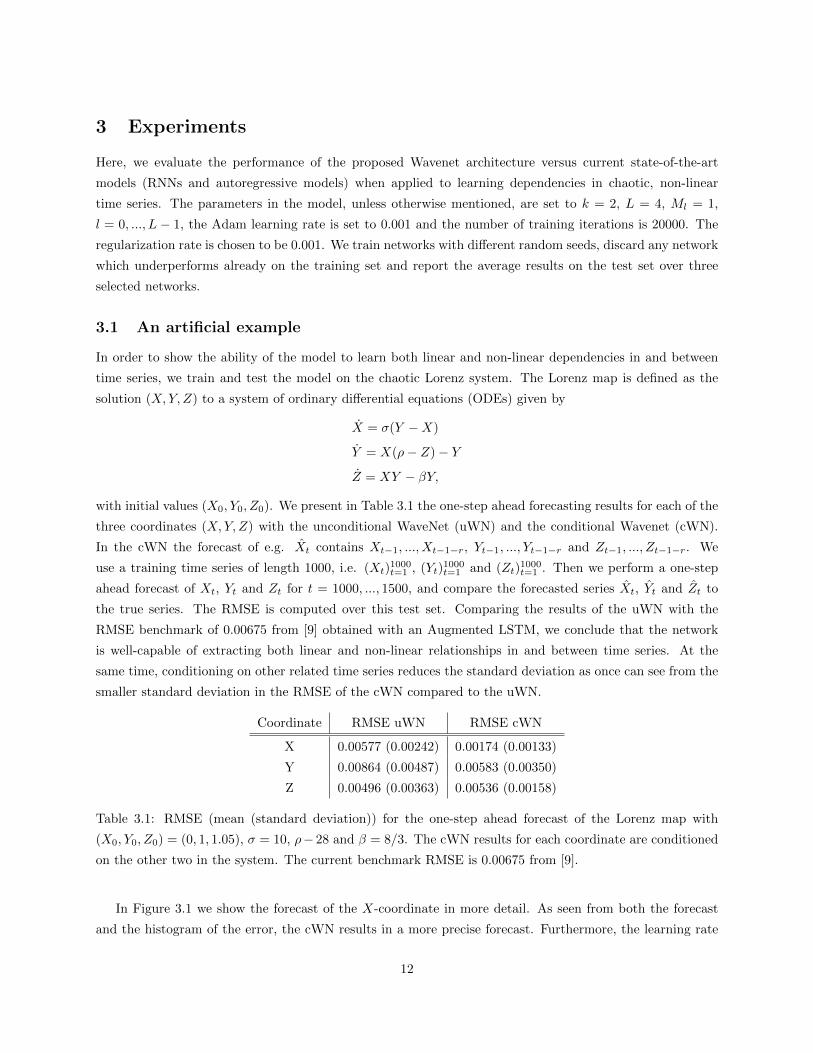
In Figure 3.1 we show the forecast of the X-coordinate in more detail. As seen from both the forecast

and the histogram of the error, the cWN results in a more precise forecast. Furthermore, the learning rate

12

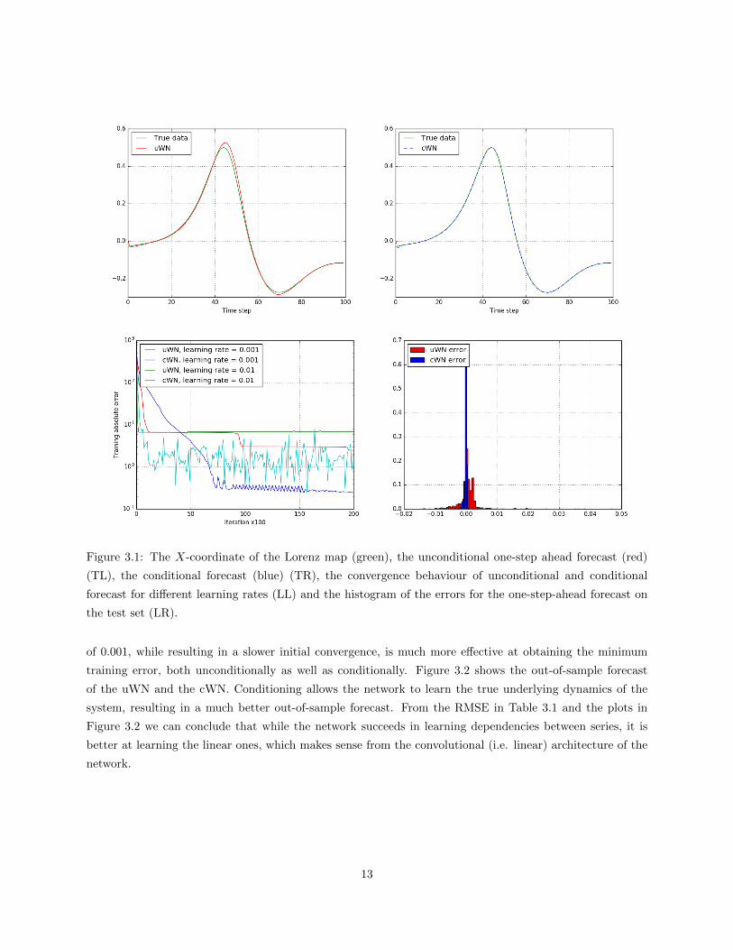
Figure 3.1: The X-coordinate of the Lorenz map (green), the unconditional one-step ahead forecast (red)

(TL), the conditional forecast (blue) (TR), the convergence behaviour of unconditional and conditional

forecast for different learning rates (LL) and the histogram of the errors for the one-step-ahead forecast on

the test set (LR).

of 0.001, while resulting in a slower initial convergence, is much more effective at obtaining the minimum

training error, both unconditionally as well as conditionally. Figure 3.2 shows the out-of-sample forecast

of the uWN and the cWN. Conditioning allows the network to learn the true underlying dynamics of the

system, resulting in a much better out-of-sample forecast. From the RMSE in Table 3.1 and the plots in

Figure 3.2 we can conclude that while the network succeeds in learning dependencies between series, it is

better at learning the linear ones, which makes sense from the convolutional (i.e. linear) architecture of the

network.

13

Figure 3.2: The training sample t ∈ [0, 1000] and a fully out-of-sample forecast for time steps t ∈ [1000, 1500]

for the X-coordinate (L) and the Y -coordinate (R)

3.2 Financial data

We analyze the performance of the network on the S&P500 data in combination with the volatility index

and the CBOE 10 year interest rate to analyze the ability of the model to extract – both unconditionally as

well as conditionally– meaningful trends from the noisy datasets. Furthermore, we test the performance on

several exchange rates.

3.2.1 Data preparation

We define a training period of 750 days (approximately three years) and a testing period of 350 days

(approximately one year) on which we perform the one-day ahead forecasting. The data from 01-01-2005

until 31-12-2016 is split into nine of these periods with non-overlapping testing periods. Let P st be the value

of time series s at time t. We define the return for s at time t over a one-day period as

Rst =

P st − P s

t−1P st−1

.

Then we normalize the returns by subtracting the mean, µtrain, and dividing by the standard deviation,

σtrain, obtained over all the time series that we will condition on in the training period (note that using the

mean and standard deviation over the train and test set would result in look-ahead biases). The normalized

return is then given by

Rst =

Rst − µtrain

σtrain.

We then divide the testing periods into three main study periods: period A from 2008 until 2010, period B

from 2011 until 2013 and period C from 2014 until 2016. The performance is then evaluated by performing

one-step ahead forecasts over these testing periods and comparing the MASE scaled by a naive forecast and

the HITS rate. An MASE smaller than one means that the absolute size of the forecasted return is more

14

accurate than that of a naive forecast, while a high HITS rate shows that the model is able to correctly

forecast the direction of the returns.

3.2.2 Benchmark models

We compare the performance of the WaveNet model with several well-known benchmarks: an autoregressive

model widely used by econometricians, and an LSTM [8][4], currently the state-of-the-art in time series

forecasting. Similar to [4] the LSTM is implemented using one LSTM layer with 25 hidden neurons and a

dropout of 0.1 followed by a fully connected output layer with one neuron and we use 500 training epochs.

LSTM networks require sequences of input features for training, and we construct the sequences using

r = 2L−1k historical time steps so that the receptive field of the WaveNet model is the same as the distance

that the LSTM can see into the past. The LSTM is implemented to take as input a matrix consisting of

sequences of all the features (the input and condition(s)), so that its performance can be compared to that

of the VAR and the cWN.

3.2.3 Results

Index forecasting We compare the performance of the unconditional and the conditional WaveNet in

forecasting the S&P500, in the cWN case conditioned on both the volatility index and the CBOE 10 year

interest rate. From Table 3.2 we see that the unconditional WaveNet performs best in terms of MASE. The

conditional WaveNet exploits the correlation between the three time series resulting in a higher hit rate, but

a slightly worse MASE compared to the unconditional one as it is fitted on multiple noisy series. The LSTM

also performs similar to the cWN in terms of the HITS rate, but results in a higher MASE, meaning that

both networks are able to forecast the direction of the returns, but the LSTM is worse at predicting the size

of the return. After 2010 the dependencies between the S&P500 and the interest rate and volatility index

seem to have weakened (due to e.g. the lower interest rate or higher spreads) as the improvement of the

conditional WaveNet over the unconditional WaveNet is smaller. This suggests that the WaveNet can be

used to recognize these switches in the underlying financial regimes. Overall, in terms of the HITS rate the

WaveNet performs similar to the state-of-the-art LSTM, in particular in period A, when strong dependencies

were still present between the index, interest rate and volatility. In the other two periods the performance

of the cWN in terms of the HITS is similar to that of a naive and the autoregressive forecast, from which we

infer that there are no longer strong dependencies present between the time series. Furthermore, the good

performance of the naive model in periods B and C can be explained by the fact that it implicitly uses the

knowledge that the period after the financial crisis was a bull market with a rising price trend. From these

results we can conclude that the WaveNet is indeed able to recognize patterns in the underlying datasets, if

these are present. If not, the WaveNet model does not overfit on the noise in the series, as can be seen by

the consistently lower MASE compared to the other models.

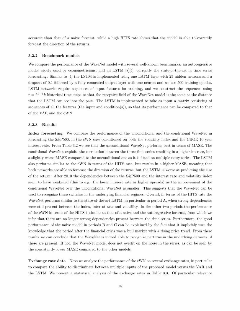
Exchange rate data Next we analyze the performance of the cWN on several exchange rates, in particular

to compare the ability to discriminate between multiple inputs of the proposed model versus the VAR and

the LSTM. We present a statistical analysis of the exchange rates in Table 3.3. Of particular relevance

15

A B C

Model MASE HITS MASE HITS MASE HITS

Naive 1 0.513 1 0.504 1 0.555

VAR 0.698 0.507 0.701 0.505 0.696 0.551

LSTM 0.873(0.026) 0.525(0.006) 1.067(0.021) 0.496(0.016) 0.929(0.021) 0.531(0.008)

uWN 0.685(0.025) 0.515(0.007) 0.681(0.002) 0.484(0.007) 0.684(0.006) 0.537(0.011)

cWN 0.699(0.042) 0.524(0.009) 0.693(0.014) 0.500(0.009) 0.701(0.015) 0.536(0.016)

Table 3.2: MASE and HITS (mean(standard deviation)) for a one-step ahead forecast over the periods A,

B and C of the S&P500, both unconditional and conditional on the volatility index and the CBOE 10 year

interest rate.

to the performance of the model are the standard deviation, skewness and kurtosis. A high standard

deviation means that there is a lot of variance in the data. This could cause models to underperform as

they become unable to accurately forecast the rapid movements. A high positive or negative skewness,

meaning the asymmetry of the returns around its mean value, indicates the existence of a long right or left

tail, respectively. We train the neural network to fit a symmetric distribution centered at the mean of the

dataset. The existence of this tail could result in the trained model performing worse in cases of high absolute

skewness. Kurtosis is a measure of the tails of the dataset compared to those of a normal distribution. A

high kurtosis is the result of infrequent extreme deviations. If a model tends to overfit the dataset, and in

particular overfit on these extreme deviations, a high kurtosis would result in a worse performance. Figure

3.3 shows the correlations between the exchange rates in the three periods. As expected, the exchange rates

that contain the same currencies exhibit stronger correlations than those with different currencies.

Stock Mean Return Standard deviation Skewness Kurtosis

A B C A B C A B C A B C

EURUSD -0.022 0.017 -0.061 1.751 0.572 0.942 0.864 0.165 0.090 25.91 1.706 1.910

EURJPY -0.050 0.053 -0.049 2.867 0.806 1.049 1.448 0.080 -0.685 43.96 1.246 5.556

GBPJPY -0.110 0.048 -0.044 2.067 0.686 1.209 -0.009 0.387 -1.129 17.23 2.743 13.45

EURGBP 0.045 0.018 -0.022 1.623 0.436 0.915 1.092 -0.229 0.444 26.60 0.606 4.919

GPBUSD -0.073 0.012 -0.058 0.975 0.453 0.895 -0.257 0.039 -1.289 1.616 0.591 15.06

Table 3.3: Statistical analysis of five foreign exchange rates.

In Table 3.4 we present the results of the conditional WaveNet forecast over the exchange rate data,

conditioning on the other exchange rates. Exchange rate data tends to contain long-term dependencies, so

we expect the WaveNet model, with its ability of learning long term relationships, to perform well. As we

see from the table, the WaveNet consistently outperforms the vector-autoregressive model and the LSTM in

terms of the MASE. In period A the data has a very high kurtosis, probably due to the global financial crisis

16

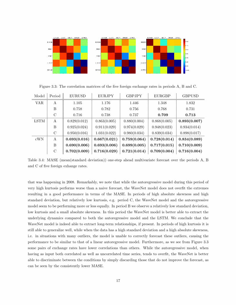
Figure 3.3: The correlation matrices of the five foreign exchange rates in periods A, B and C.

Model Period EURUSD EURJPY GBPJPY EURGBP GBPUSD

VAR A 1.105 1.176 1.446 1.348 1.832

B 0.758 0.782 0.756 0.768 0.731

C 0.716 0.738 0.737 0.709 0.713

LSTM A 0.829(0.012) 0.863(0.005) 0.880(0.004) 0.868(0.005) 0.893(0.007)

B 0.925(0.024) 0.911(0.029) 0.974(0.029) 0.948(0.023) 0.934(0.014)

C 0.950(0.016) 1.031(0.022) 0.980(0.034) 0.839(0.034) 0.898(0.017)

cWN A 0.693(0.016) 0.667(0.021) 0.759(0.064) 0.728(0.014) 0.834(0.089)

B 0.690(0.006) 0.693(0.006) 0.699(0.005) 0.717(0.015) 0.710(0.009)

C 0.702(0.009) 0.716(0.029) 0.721(0.014) 0.709(0.004) 0.716(0.004)

Table 3.4: MASE (mean(standard deviation)) one-step ahead multivariate forecast over the periods A, B

and C of five foreign exhange rates.

that was happening in 2008. Remarkably, we note that while the autoregressive model during this period of

very high kurtosis performs worse than a naive forecast, the WaveNet model does not overfit the extremes

resulting in a good performance in terms of the MASE. In periods of high absolute skewness and high

standard deviation, but relatively low kurtosis, e.g. period C, the WaveNet model and the autoregressive

model seem to be performing more or less equally. In period B we observe a relatively low standard deviation,

low kurtosis and a small absolute skewness. In this period the WaveNet model is better able to extract the

underlying dynamics compared to both the autoregressive model and the LSTM. We conclude that the

WaveNet model is indeed able to extract long-term relationships, if present. In periods of high kurtosis it is

still able to generalize well, while when the data has a high standard deviation and a high absolute skewness,

i.e. in situations with many outliers, the model is unable to correctly forecast these outliers, causing the

performance to be similar to that of a linear autoregressive model. Furthermore, as we see from Figure 3.3

some pairs of exchange rates have lower correlations than others. While the autoregressive model, when

having as input both correlated as well as uncorrelated time series, tends to overfit, the WaveNet is better

able to discriminate between the conditions by simply discarding those that do not improve the forecast, as

can be seen by the consistently lower MASE.

17

4 Discussion and conclusion

In this paper we presented and analysed the performance of a method for conditional time series forecasting

based on a convolutional neural network known as the WaveNet architecture [13]. The network makes use

layers of dilated convolutions applied to the input and multiple conditions, in this way learning the trends

and relations in and between the data. We analysed the performance of the WaveNet model on various time

series, and compared the performance with the current state-of-the-art method in time series forecasting,

the LSTM model, and a linear autoregressive model. We conclude that even though time series forecasting

remains a complex task and finding one model that fits all is hard, we have shown that the WaveNet is a

simple, efficient and easily interpretable network that can act as a strong baseline for forecasting. Nevertheless

there is still room for improvement. As we saw in the example in Section 3.1, while summing the convolved

condition with the convolved input after the first layer allowed the network to learn (weakly non-) linear

relationships in the data, the results suggest that one might design a network that is better able of extracting

non-linear dynamics by e.g. computing the product at each location between the input and the condition

with an outer product. Furthermore, the WaveNet model proved to be a strong competitor to LSTM models,

in particular when taking into consideration the training time. While on the relatively short time series the

prediction time is negligible when compared to the training time, for longer time series the prediction of the

autoregressive model may be sped up by implementing a recent variation that exploits the memorization

structure of the network, see [12]. Finally, it is well-known that correlations between data points are stronger

on an intraday basis. Therefore, it might be interesting to test the model on intraday data to see if the

ability of the model to learn long-term dependencies is even more valuable in that case.

Acknowledgements

This research is supported by the European Union in the the context of the H2020 EU Marie Curie Initial

Training Network project named WAKEUPCALL

References

[1] Y. Bengio, P. Simard, and P. Frasconi, Learning Long-Term Dependencies with Gradient Descent

is Difficult, IEEE Transactions on Neural Networks, 5 (1994).

[2] M. Binkowski, G. Marti, and P. Donnat, Autoregressive convolutional neural networks for asyn-

chronous time series, ICML 2017 Time Series Workshop, (2017).

[3] K. Chakraborty, K. Mehrotra, C. K. Mohan, and S. Ranka, Forecasting the Behavior of

Multivariate Time Series using Neural Networks, Neural networks, 5 (1992), pp. 961–970.

[4] T. Fisher and C. Krauss, Deep learning with long short-term memory networks for financial market

predictions, FAU Discussion papers in Economics, (2017).

18

[5] X. Glorot and Y. Bengio, Understanding the Difficulty of Training Deep Feedforward Neural Net-

works, Proceedings of the 13th International Conference on Artificial Intelligence and Statistics, (2010).

[6] K. He, X. Zhang, S. Ren, and J. Sun, Delving deep into rectifiers: Surpassing human-level per-

formance on imagenet classification, in Proceedings of the IEEE international conference on computer

vision, 2015, pp. 1026–1034.

[7] , Deep residual learning for image recognition, in Proceedings of the IEEE conference on computer

vision and pattern recognition, 2016, pp. 770–778.

[8] S. Hochreiter and J. Schmidhuber, Long short- term memory, Neural computation, 9 (1997),

pp. 1735–1780.

[9] D. Hsu, Time series forecasting based on augmented long short-term memory, arXiv preprint

arXiv:1707.00666, (2017).

[10] D. Kingma and J. Ba, Adam: A method for stochastic optimization, arXiv preprint arXiv:1412.6980,

(2014).

[11] A. Krizhevsky, I. Sutskever, and G. E. Hinton, ImageNet Classification with Deep Convolutional

Neural Networks, Advances in Neural Information Processing Systems 25, (2012), pp. 1097–1105.

[12] P. Ramachandran, T. L. Paine, P. Khorrami, M. Babaeizadeh, S. Chang, Y. Zhang, M. A.

Hasegawa-Johnson, R. H. Campbell, and T. S. Huang, Fast generation for convolutional autore-

gressive models, arXiv preprint arXiv:1704.06001, (2017).

[13] A. van den Oord, S. Dieleman, H. Zen, K. Simonyan, O. Vinyals, A. Graves, N. Kalch-

brenner, A. Senior, and K. Kavukcuoglu, WaveNet: A Generative Model for Raw Audio, ArXiv

e-prints, (2016).

[14] A. van den Oord, N. Kalchbrenner, O. Vinyals, L. Espeholt, A. Graves, and

K. Kavukcuoglu, Conditional Image Generation with PixelCNN Decoders, CoRR, abs/1606.05328

(2016).

[15] Z. Wang, W. Yan, and T. Oates, Time Series Classification from Scratch with Deep Neural Net-

works: A Strong Baseline, CoRR, abs/1611.06455 (2016).

[16] F. Yu and V. Koltun, Multi-Scale Context Aggregation by Dilated Convolutions, ArXiv e-prints,

(2015).

19