Embed Size (px)
Citation preview

1
AGEC 603
Production and Cost Relationships
• Homogeneous products
– Products from different producers are perfect
substitutes
• No barriers to entry or exit
– Resources are free to move in and out of the sector
• Large number of buyers and sellers
– No market power – price takers
• Perfect information
– Including quantities, prices, quality, sources of
resources etc.
Conditions for Perfect
Competition
• Land - includes renewable (forests) and non-
renewable (minerals) resources
• Labor - all owner and hired labor services,
excluding management
• Capital - manufactured goods such as fuel,
chemicals, tractors and buildings
• Management - production decisions
designed to achieve specific economic goal
Classification of Inputs
2
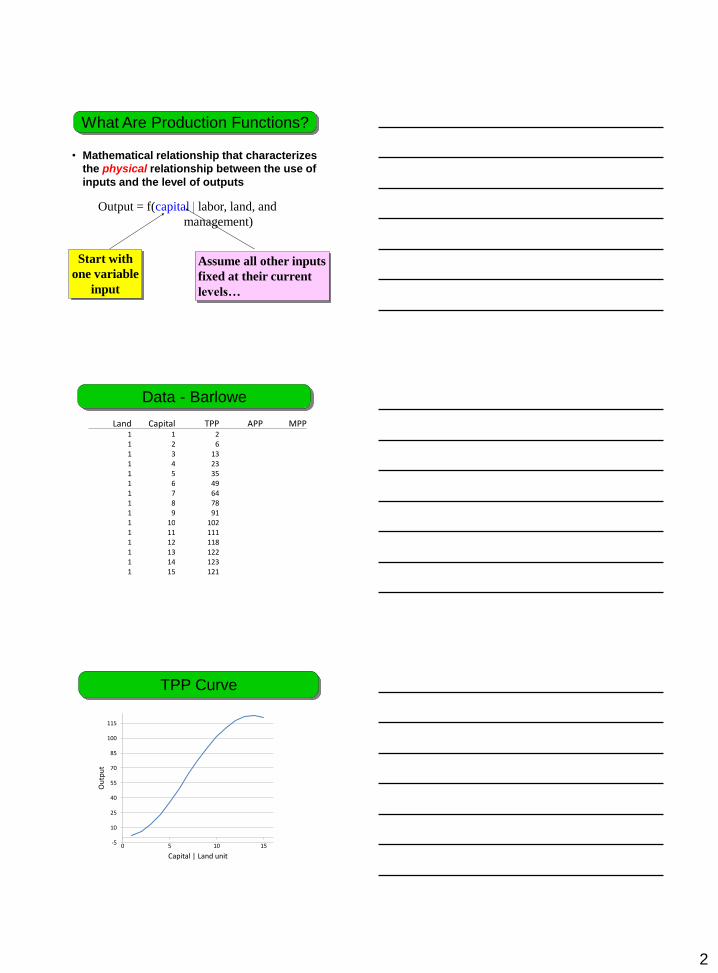
• Mathematical relationship that characterizes
the physical relationship between the use of
inputs and the level of outputs
What Are Production Functions?
Output = f(capital | labor, land, and
management)
Start with
one variable
input
Assume all other inputs
fixed at their current
levels…
Data - Barlowe
Land Capital TPP APP MPP1 1 21 2 61 3 131 4 231 5 351 6 491 7 641 8 781 9 911 10 1021 11 1111 12 1181 13 1221 14 1231 15 121
TPP Curve
-5
10
25
40
55
70
85
100
115
0 5 10 15
Ou
tpu
t
Capital | Land unit
3
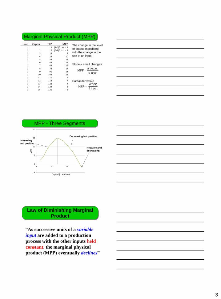
The change in the level
of output associated
with the change in the
use of an input.
Slope – small changes
Partial derivative
MPP =𝛿 𝑇𝑃𝑃
𝛿 input
Marginal Physical Product (MPP)
input
outputMPP
Land Capital TPP MPP1 1 2 (2-0)/(1-0) = 21 2 6 (6-2)/(2-1) = 41 3 13 71 4 23 101 5 35 121 6 49 141 7 64 151 8 78 141 9 91 131 10 102 111 11 111 91 12 118 71 13 122 41 14 123 11 15 121 -2
-5
0
5
10
15
20
0 5 10 15
MP
P
Capital | Land unit
MPP - Three Segments
Increasing
and positive
Decreasing but positive
Negative and
decreasing
“As successive units of a variable
input are added to a production
process with the other inputs held
constant, the marginal physical
product (MPP) eventually declines”
Law of Diminishing Marginal
Product

4
• Represents the
output per unit of
input
Average Physical Product (APP)
inputtotal
outputtotalAPP
Land Capital TPP APP1 1 2 2/1 = 2.0001 2 6 6/2 = 3.0001 3 13 13/3 = 4.3331 4 23 5.7501 5 35 7.0001 6 49 8.1671 7 64 9.1431 8 78 9.7501 9 91 10.1111 10 102 10.2001 11 111 10.0911 12 118 9.8331 13 122 9.3851 14 123 8.7861 15 121 8.067
0
5
10
15
20
0 5 10 15
AP
P
Capital | Land unit
APP Graphically
Increasing and positive Decreasing
but never goes negative
Data
Land Capital TPP APP MPP1 1 2 2.000 21 2 6 3.000 41 3 13 4.333 71 4 23 5.750 101 5 35 7.000 121 6 49 8.167 141 7 64 9.143 151 8 78 9.750 141 9 91 10.111 131 10 102 10.200 111 11 111 10.091 91 12 118 9.833 71 13 122 9.385 41 14 123 8.786 11 15 121 8.067 -2
5
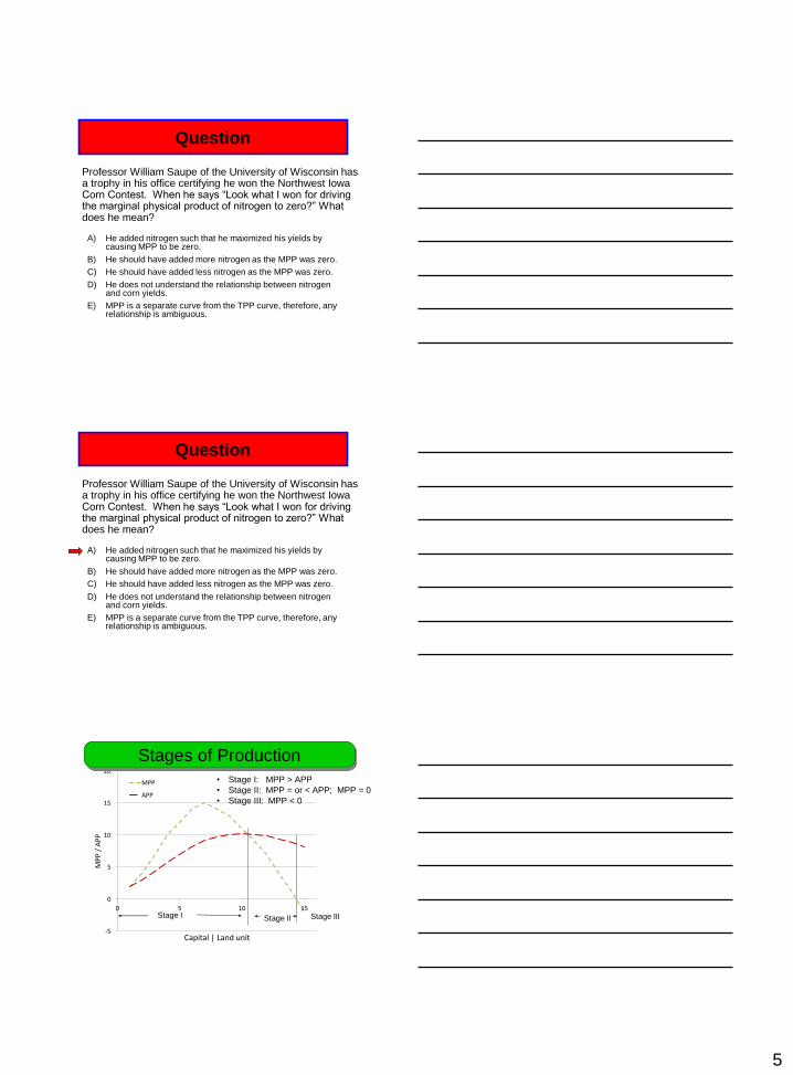
Professor William Saupe of the University of Wisconsin has a trophy in his office certifying he won the Northwest Iowa Corn Contest. When he says “Look what I won for driving the marginal physical product of nitrogen to zero?” What does he mean?
Question
A) He added nitrogen such that he maximized his yields by causing MPP to be zero.
B) He should have added more nitrogen as the MPP was zero.
C) He should have added less nitrogen as the MPP was zero.
D) He does not understand the relationship between nitrogen and corn yields.
E) MPP is a separate curve from the TPP curve, therefore, any relationship is ambiguous.
-5
0
5
10
15
20
0 5 10 15
MP
P /
AP
P
Capital | Land unit
MPP
APP
Stages of Production
Stage I Stage II Stage III
• Stage I: MPP > APP
• Stage II: MPP = or < APP; MPP = 0
• Stage III: MPP < 0

6
-5
10
25
40
55
70
85
100
115
0 5 10 15
Ou
tpu
t
Capital | Land unit
TPP
APP
MPP
Relationships - Know
TPP
MPP
APP
Stage I
Stage II
Stage III
Assume a firm is producing where the MPP is negative. At this point of production, we know the APP and TPP curves are
Question
A) Both are negative.
B) One is negative and the other is positive but the relationship is unknown without further information.
C) Production is elastic at this point.
D) TPP is negative and APP is positive.
E) Both positive.
Assume a firm is producing where the MPP is negative. At this point of production, we know the APP and TPP curves are
Question
-15
-10
-5
0
5
10
15
20
25
30
35
0 2 4 6 8 10 12
Pickers per Day
Co
rn d
oze
n ~
0
20
40
60
80
100
120
140
160
0 2 4 6 8 10 12
Co
rn D
ozen
`
Stage IIIStage IIStage I
0
20
40
60
80
100
120
140
160
0 2 4 6 8 10 12
Positive
TPP
Positive
APP
A) Both are negative.
B) One is negative and the other is positive but the relationship is unknown without further information.
C) Production is elastic at this point.
D) TPP is negative and APP is positive.
E) Both positive. APP and TPP are always positive. KNOW WHY?
7
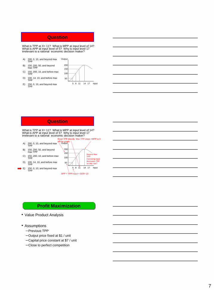
What is TPP at X= 11? What is MPP at input level of 14? What is APP at input level of 5? Why is input level 17 irrelevant to a rational economic decision maker?
Question
A) 200, 0, 10, and beyond max TPP
B) 150, 200, 50, and beyond max TPP
C) 150, 200, 10, and before max TPP
D) 100, 14, 10, and before max TPP
E) 150, 0, 10, and beyond max TPP
5 8 11 14 17 input
Output
200
150
100
50
Max TPP slope =MPP is 0
APP = TPP/ input = 50/5= 10
Read TPP directly
off the graph
Beyond Max
TPP
Increasing input
decreases TPP
so why use?
• Value Product Analysis
• Assumptions
–Previous TPP
–Output price fixed at $1 / unit
–Capital price constant at $7 / unit
–Close to perfect competition
Profit Maximization

8
TVP
LandCapital TPP APP MPP TVP1 1 2 2.000 2 1*2 = 21 2 6 3.000 4 1*6 = 61 3 13 4.333 7 131 4 23 5.750 10 231 5 35 7.000 12 351 6 49 8.167 14 491 7 64 9.143 15 641 8 78 9.750 14 781 9 91 10.111 13 911 10 102 10.200 11 1021 11 111 10.091 9 1111 12 118 9.833 7 1181 13 122 9.385 4 1221 14 123 8.786 1 1231 15 121 8.067 -2 121
TVP = price * TPP
Note price = $1
Not generally the case
MVP
LandCapital TPP APP MPP TVP MVP1 1 2 2.000 2 2 1*2 = 21 2 6 3.000 4 6 1*4 = 41 3 13 4.333 7 13 71 4 23 5.750 10 23 101 5 35 7.000 12 35 121 6 49 8.167 14 49 141 7 64 9.143 15 64 151 8 78 9.750 14 78 141 9 91 10.111 13 91 131 10 102 10.200 11 102 111 11 111 10.091 9 111 91 12 118 9.833 7 118 71 13 122 9.385 4 122 41 14 123 8.786 1 123 11 15 121 8.067 -2 121 -2
MVP = price * MPP
or change in TVP / change
in input
Marginal return per unit of
input
Note price = $1
Not generally the case
AVP
Land Capital TPP APP MPP TVPMVP AVP1 1 2 2.000 2 2 2 1*2 = 21 2 6 3.000 4 6 4 1*3 = 31 3 13 4.333 7 13 7 4.3331 4 23 5.750 10 23 10 5.7501 5 35 7.000 12 35 12 7.0001 6 49 8.167 14 49 14 8.1671 7 64 9.143 15 64 15 9.1431 8 78 9.750 14 78 14 9.7501 9 9110.111 13 91 13 10.1111 10 10210.200 11 102 11 10.2001 11 11110.091 9 111 9 10.0911 12 118 9.833 7 118 7 9.8331 13 122 9.385 4 122 4 9.3851 14 123 8.786 1 123 1 8.7861 15 121 8.067 -2 121 -2 8.067
AVP = price * APP or
TVP / total input
Note price = $1
Not generally the
case

9
Total Variable Cost - TVC
Land Capital TPP APP MPP TVP MVP AVP TC1 1 2 2.000 2 2 2 1*2 = 2 7*1 = 71 2 6 3.000 4 6 4 1*3 = 3 7*2 = 141 3 13 4.333 7 13 7 4.333 211 4 23 5.750 10 23 10 5.750 281 5 35 7.000 12 35 12 7.000 351 6 49 8.167 14 49 14 8.167 421 7 64 9.143 15 64 15 9.143 491 8 78 9.750 14 78 14 9.750 561 9 91 10.111 13 91 13 10.111 631 10 102 10.200 11 102 11 10.200 701 11 111 10.091 9 111 9 10.091 771 12 118 9.833 7 118 7 9.833 841 13 122 9.385 4 122 4 9.385 911 14 123 8.786 1 123 1 8.786 981 15 121 8.067 -2 121 -2 8.067 105
TC
= p
rice o
f input * in
put le
vel
AFC and MFC
Land Capital TPP APP MPP TVP MVP AVP TC AFC MFC1 1 2 2.000 2 2 2 1*2 = 2 7 7/1 = 7 7/1 = 7
1 2 6 3.000 4 6 4 1*3 = 3 14 14/2 = 7(14-7)/ (2-1)=7
1 3 13 4.333 7 13 7 4.333 21 7 71 4 23 5.750 10 23 10 5.750 28 7 71 5 35 7.000 12 35 12 7.000 35 7 71 6 49 8.167 14 49 14 8.167 42 7 71 7 64 9.143 15 64 15 9.143 49 7 71 8 78 9.750 14 78 14 9.750 56 7 71 9 91 10.111 13 91 13 10.111 63 7 71 10 102 10.200 11 102 11 10.200 70 7 71 11 111 10.091 9 111 9 10.091 77 7 71 12 118 9.833 7 118 7 9.833 84 7 71 13 122 9.385 4 122 4 9.385 91 7 71 14 123 8.786 1 123 1 8.786 98 7 71 15 121 8.067 -2 121 -2 8.067 105 7 7
MFC = marginal factor cost = additional cost
associated with the application of each
successive variable input = ∆ in TC / ∆ input
AFC = average factor cost = cost per unit of input
= TC / input level
In this case the AFC = MFC = constant = $7
Why?
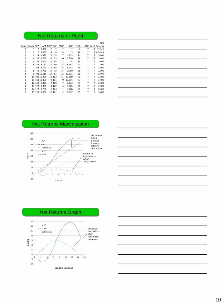
Net Returns or Profit
Land Capital TPP APP MPP TVP MVP AVP TC AFC MFCNet
Returns
1 1 2 2.000 2 2 2 2 7 7 7 2-7=-51 2 6 3.000 4 6 4 3 14 7 7 6-14=-81 3 13 4.333 7 13 7 4.333 21 7 7 -8.001 4 23 5.750 10 23 10 5.750 28 7 7 -5.001 5 35 7.000 12 35 12 7. 35 7 7 0.001 6 49 8.167 14 49 14 8.167 42 7 7 7.001 7 64 9.143 15 64 15 9.143 49 7 7 15.001 8 78 9.750 14 78 14 9.750 56 7 7 22.001 9 91 10.111 13 91 13 10.111 63 7 7 28.001 10 102 10.200 11 102 11 10.200 70 7 7 32.001 11 111 10.091 9 111 9 10.091 77 7 7 34.001 12 118 9.833 7 118 7 9.833 84 7 7 34.001 13 122 9.385 4 122 4 9.385 91 7 7 31.001 14 123 8.786 1 123 1 8.786 98 7 7 25.001 15 121 8.067 -2 121 -2 8.067 105 7 7 16.00
Net Returns = TVP – TC
10
Net Returns or Profit
Land Capital TPP APP MPP TVP MVP AVP TVC AFC MFCNet
Returns
1 1 2 2.000 2 2 2 2 7 7 7 2-7=-51 2 6 3.000 4 6 4 3 14 7 7 6-14=-81 3 13 4.333 7 13 7 4.333 21 7 7 -8.001 4 23 5.750 10 23 10 5.750 28 7 7 -5.001 5 35 7.000 12 35 12 7. 35 7 7 0.001 6 49 8.167 14 49 14 8.167 42 7 7 7.001 7 64 9.143 15 64 15 9.143 49 7 7 15.001 8 78 9.750 14 78 14 9.750 56 7 7 22.001 9 91 10.111 13 91 13 10.111 63 7 7 28.001 10 102 10.200 11 102 11 10.200 70 7 7 32.001 11 111 10.091 9 111 9 10.091 77 7 7 34.001 12 118 9.833 7 118 7 9.833 84 7 7 34.001 13 122 9.385 4 122 4 9.385 91 7 7 31.001 14 123 8.786 1 123 1 8.786 98 7 7 25.001 15 121 8.067 -2 121 -2 8.067 105 7 7 16.00
-20
0
20
40
60
80
100
120
140
0 2 4 6 8 10 12 14 16
Do
llars
Captial
TVP
TVC
Net Returns
MFC
MVP
Net Returns Maximization
Net returns
max at
greatest
distance
between
TVP and TC
Occurs at
input level in
which
MFC = MVP
-10
-5
0
5
10
15
20
25
30
35
0 2 4 6 8 10 12 14 16
Do
llars
Capital | Land unit
MFC
MVP
Net Returns
Net Returns Graph
Input level
that MFC =
MVP
maximizes
net returns

11
• Fixed costs – do not vary with the level
of input use
• Variable costs – vary with the level of
input use
• Similar to production can obtain curves
such as total, average, and marginal
costs
Short-Run Costs
• Fixed costs = 0 in Barlowe
• With only two inputs, land and capital the
profits we are generating are returns to
the fixed input – land
• Usually TC = TVC + FC but our case
–FC = 0, therefore TC = TVC
• OK
–returns to land
–fixed costs do not influence decision making
Note on Fixed Costs
Total Costs
• Recall capital costs = $7 / unit
Land Capital TPP FC TVC FC+TVC =TC1 1 2 0 1 * 7 = 7 0 + 7 = 71 2 6 0 2 * 7 = 14 0 + 14 = 141 3 13 0 3 * 7 = 21 211 4 23 0 28 281 5 35 0 35 351 6 49 0 42 421 7 64 0 49 491 8 78 0 56 561 9 91 0 63 631 10 102 0 70 701 11 111 0 77 771 12 118 0 84 841 13 122 0 91 911 14 123 0 98 981 15 121 0 105 105
Note,
Will ignore
Land and FC
in proceeding
slides!

12
Total Costs - Graphically
0
20
40
60
80
100
120
Do
llars
Output or TPP
After max TTP decreases
but costs still increase.
Produce in Stage III?
Cost increase at
increasing rate.
Cost increase at
decreasing rate.
Average / Marginal Costs• Average cost = total cost / output
• Marginal cost = change in total costs / change in output
Capital TPP TC ATC MC1 2 7 7/2 = 3.50 (7-0)/(2-0) = 3.502 6 14 14/6 = 2.33 (14-7)/(6-2) = 1.753 13 21 21/13 = 1.62 (21-14)/(13-6) = 1.004 23 28 1.22 0.705 35 35 1.00 0.586 49 42 0.86 0.507 64 49 0.77 0.478 78 56 0.72 0.509 91 63 0.69 0.54
10 102 70 0.69 0.6411 111 77 0.69 0.7812 118 84 0.71 1.0013 122 91 0.75 1.7514 123 98 0.80 7.0015 121 105 0.87 -3.50
Why MC is
not relevant
in stage III!
Marginal / Average Costs
0.00
1.00
2.00
3.00
4.00
5.00
6.00
7.00
8.00
Do
llars
Output or TPP
MC
AC
13
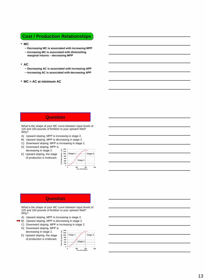
• MC
– Decreasing MC is associated with increasing MPP
– Increasing MC is associated with diminishing
marginal returns – decreasing MPP
• AC
– Decreasing AC is associated with increasing APP
– Increasing AC is associated with decreasing APP
• MC = AC at minimum AC
Cost / Production Relationships
What is the shape of your MC curve between input levels of 125 and 150 pounds of fertilizer to your spinach field? Why?
A) Upward sloping, MPP is increasing is stage 2.
B) Upward sloping, MPP is decreasing in stage 2.
C) Downward sloping, MPP is increasing in stage 2.
D) Downward sloping, MPP is
decreasing in stage 2.
E) Upward sloping, the stage
of production is irrelevant.
Question
Stage 1
Stage 2
Stage 3

14
Net Returns = TVP - TC
0
20
40
60
80
100
120
140
Do
llars
Output or TPP
TC
TVP
Net returns
max at
greatest
distance
between
TVP and TC
Similar to what we have been doing
• Total Revenue (TVP) = price x quantity – WHY?
• Average Revenue – revenue per unit of output
• Marginal Revenue – change in total revenue as
output changes
• Objective maximize net returns given fixed land
unit
Short-Run Decisions
output
revenueMR
outputtotal
revenuetotalAR
Average / Marginal Revenues
• Recall price of $1
TPP TPP * price = TR AR MR2.00 2 * 1 = 2.00 2/2 = 1.00 (2-0)/(2-0) = 16.00 6* 1 = 6.00 6/6 = 1.00 (6-2)/(6-2) = 1
13.00 13.00 1.00 123.00 23.00 1.00 135.00 35.00 1.00 149.00 49.00 1.00 164.00 64.00 1.00 178.00 78.00 1.00 191.00 91.00 1.00 1
102.00 102.00 1.00 1111.00 111.00 1.00 1118.00 118.00 1.00 1122.00 122.00 1.00 1123.00 123.00 1.00 1121.00 121.00 1.00 1
𝐴𝑅 = 𝑇𝑅/𝑇𝑃𝑃 M𝑅 = Δ𝑇𝑅/𝛥𝑇𝑃𝑃

15
• Perfect competition in the short run produce at the point
MC = MR
Level of Output MC = MR
Net revenue
maximizing
point MC = MR
0.00
1.00
2.00
3.00
4.00
5.00
6.00
7.00
Do
llars
Output or TPP
MC
AC
MR
• Why? Examine MR and MC curves
Level of Output MC = MR
MC
MR
MCb
MCA
MC < MR
Produce more – Why?
MC > MR
Produce less – Why?
MC = MR
Correct output level – Why?
TR and TC Areas
Note change in y-axis for clarity
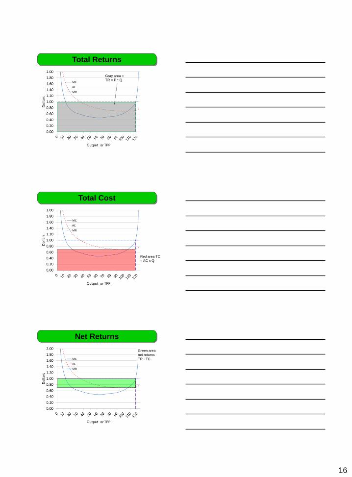
16
Total Returns
Gray area =
TR = P * Q
Total Cost
Red area TC
= AC x Q
Net Returns
Green area
net returns
TR - TC

17
• Breakeven price - price that just covers total costs
• TR = TC implies economic profits are zero
Breakeven Price
Price = $0.69
= min AC
• Breakeven price - price that just covers total costs
• TR = TC implies economic profits are zero
Breakeven Price
Gray area TR
Price = $0.69
= min AC
• Breakeven price - price that just covers total costs
• TR = TC implies economic profits are zero
Breakeven Price
Price = $0.69
= min AC
Red area TC
Notice
profits = 0
18
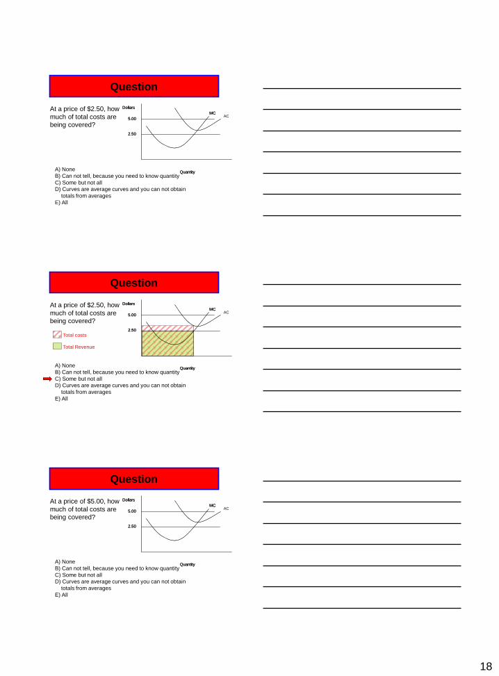
At a price of $2.50, how
much of total costs are
being covered?
Question
A) None
B) Can not tell, because you need to know quantity
C) Some but not all
D) Curves are average curves and you can not obtain
totals from averages
E) All
Quantity
5.00
2.50
MCAC
Dollars
Quantity
5.00
2.50
MC
Dollars
At a price of $2.50, how
much of total costs are
being covered?
Question
A) None
B) Can not tell, because you need to know quantity
C) Some but not all
D) Curves are average curves and you can not obtain
totals from averages
E) All
Total costs
Total Revenue
Quantity
5.00
2.50
MCAC
Dollars
Quantity
5.00
2.50
MC
Dollars
At a price of $5.00, how
much of total costs are
being covered?
Question
A) None
B) Can not tell, because you need to know quantity
C) Some but not all
D) Curves are average curves and you can not obtain
totals from averages
E) All
Quantity
5.00
2.50
MCAC
Dollars
Quantity
5.00
2.50
MC
Dollars
19
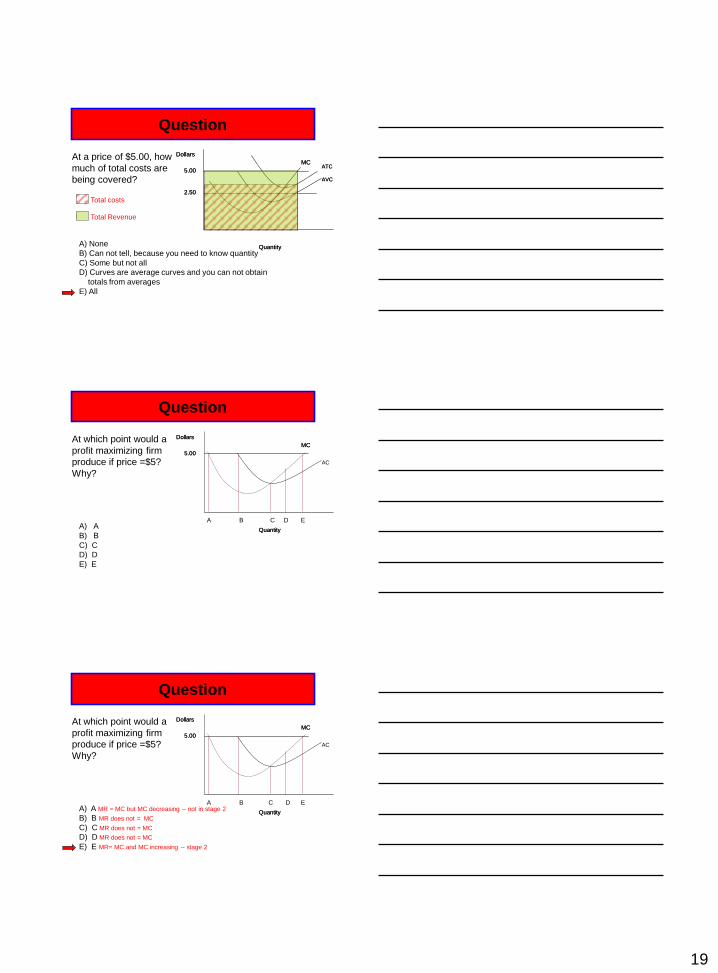
At a price of $5.00, how
much of total costs are
being covered?
Question
Quantity
5.00
2.50
MCATC
AVC
Dollars
Quantity
5.00
2.50
MCATC
AVC
Dollars
A) None
B) Can not tell, because you need to know quantity
C) Some but not all
D) Curves are average curves and you can not obtain
totals from averages
E) All
Total costs
Total Revenue
At which point would a
profit maximizing firm
produce if price =$5?
Why?
Question
A) A
B) B
C) C
D) D
E) E
Quantity
5.00
MC
AC
Dollars
Quantity
5.00
MC
Dollars
A B C D E
At which point would a
profit maximizing firm
produce if price =$5?
Why?
Question
A) A MR = MC but MC decreasing -- not in stage 2
B) B MR does not = MC
C) C MR does not = MC
D) D MR does not = MC
E) E MR= MC and MC increasing -- stage 2
Quantity
5.00
MC
AC
Dollars
Quantity
5.00
MC
Dollars
A B C D E
20
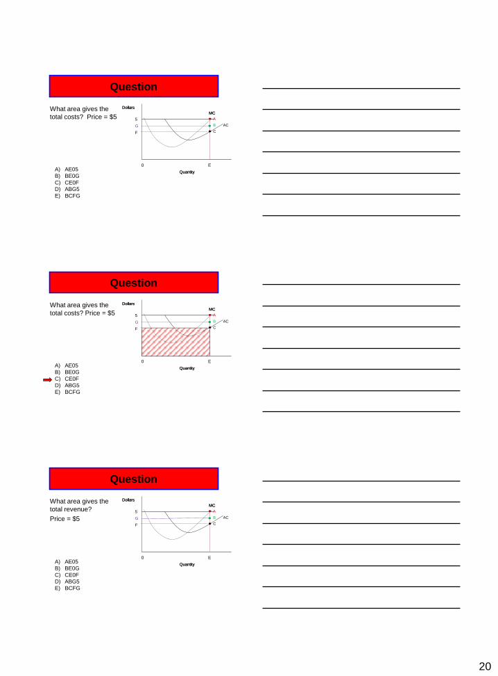
What area gives the
total costs? Price = $5
Question
Quantity
5
G
F
MC
AC
Dollars
Quantity
MC
Dollars
0 E
A
B
C
A) AE05
B) BE0G
C) CE0F
D) ABG5
E) BCFG
What area gives the
total costs? Price = $5
Question
Quantity
5
G
F
MC
AC
Dollars
Quantity
MC
Dollars
0 E
A
B
C
A) AE05
B) BE0G
C) CE0F
D) ABG5
E) BCFG
What area gives the
total revenue?
Price = $5
Question
Quantity
5
G
F
MC
AC
Dollars
Quantity
MC
Dollars
0 E
A
B
C
A) AE05
B) BE0G
C) CE0F
D) ABG5
E) BCFG

21
What area gives the
total revenue?
Price = $5
Question
A) AE05
B) BE0G
C) CE0F
D) ABG5
E) BCFG
Quantity
5
G
F
MC
AVC
Dollars
Quantity
MC
AVC
Dollars
0 E
A
B
C
What area gives profits?
Price = $5
Question
Quantity
5
G
F
MC
AC
Dollars
Quantity
MC
Dollars
0 E
A
B
C
A) AE05
B) BE0G
C) CE0F
D) ABG5
E) BCFG
A) AE05
B) BE0G
C) CE0F
D) ACF5
E) BCFG
What area gives profits?
Question
Quantity
5
G
F
MC
AC
Dollars
Quantity
MC
Dollars
0 E
A
B
C

22
• Land the fixed factor
– Short Run - land usually assumed fixed
– Long Run - land is variable
• Define economic land use
• Intensity
– Refers to the relative amount of capital and labor
combined with units of land in the production process -
relative amounts of capital and labor
• high ratio implies intensive use
• downtown vs. ranch
• Two Concepts
– Intensive margin
– Extensive margin
Intensity of Land Use
• Concept applies to all uses of land
• Intensive Margin
– Input level associated with maximizing net returns
• MFC = MVP or
• MC = MR
Intensive Margin of Land
We will concentrate on cost curves
Give same point
MR
5
10
15
20
25
30
5 10 15 20 25 30 35 40 450
MC
AC
Pri
ce
Output
Intensive Margin – Good
Area of insufficient input use Area of too much input use
Intensive margin
Green box = net returnsProduce at MR = MC
Assume occurs at 15 units of capital
23
MR
5
10
15
20
25
30
5 10 15 20 25 30 35 40 450
AC
PR
ICE
Output
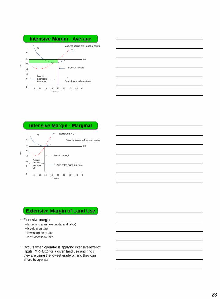
Intensive Margin - Average
Area of
insufficient
input use Area of too much input use
Intensive margin
MC
Assume occurs at 10 units of capital
MR
5
10
15
20
25
30
5 10 15 20 25 30 35 40 450
AC
PR
ICE
Output
Intensive Margin - Marginal
Area of
insuffici
ent input
use
Area of too much input use
Intensive margin
MC
Assume occurs at 5 units of capital
Net returns = 0
• Extensive margin
– large land area (low capital and labor)
– break even tract
– lowest grade of land
– least accessible site
• Occurs when operator is applying intensive level of
inputs (MR=MC) for a given land use and finds
they are using the lowest grade of land they can
afford to operate
Extensive Margin of Land Use

24
Extensive Margin
AC
MR
Pri
ce
Output
MC
AC
MR
Pri
ce
Output
MC AC
MR
Pri
ce
Output
MC
Good Average Marginal
Intensive margins Extensive margin
Decreasing Land Capacity
Eco
no
mic
Cap
acit
y o
f La
nd
Continuum
15
10
5
Good Average Marginal
Intensive margins
Extensive margin
Decreasing Land Capacity
Eco
no
mic
Cap
acit
y o
f La
nd
Continuum
15
10
5
Good Average Marginal
Intensive margins for
Best land
Sub average land
25
Decreasing Land Capacity
Eco
no
mic
Cap
acit
y o
f La
nd 15
10
5
Good Average Marginal
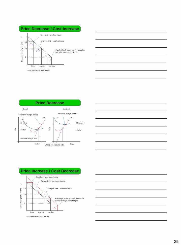
Marginal land – taken out of productionExtensive margin shifts to left
Price Decrease / Cost Increase
Good land – uses less inputs
Average land – uses less inputs
Price Decrease
AC
MR before
Pri
ce
Output
MCAC
MR before
Pri
ce
Output
MC
Good Marginal
Intensive margin beforeIntensive margin before
MR after
Intensive margin after
MR after
Would not produce after
Price Increase / Cost Decrease
Decreasing Land Capacity
Eco
no
mic
Cap
acit
y o
f La
nd 15
10
5
Good Average Marginal
Sub marginal land –put into productionExtensive margin shifts to right
Good land – uses more inputs
Average land – uses more inputs
Marginal land – uses more inputs

26
Price Increase
AC
MR beforePri
ce
Output
MC
ACMR before
Pri
ce
Output
MC
Good Sub marginal
Intensive margin afterIntensive margin after
MR after
Intensive margin before
MR after
Intensive margin before
Not producing
• Type of use
– Commercial vs. residential vs. farming
– Technology
• For a given use– Characteristics of the land
– Changing economic conditions
– Owners expectations and attitudes
– Technology
Factors Influencing Intensity
• Equi-marginal principle
• If a resources is limited, maximum net returns
occur when MVP is at least equal to the next
best alternative (opportunity cost)
• MVP will be equal
• Example
• Assumptions• Three tracts of land - not homogenous
• 30 units of the input available
• TVP and MVP varying between the tracts – next table
• Input costs = $3 / unit = MFC
Equi-marginal Principle
27
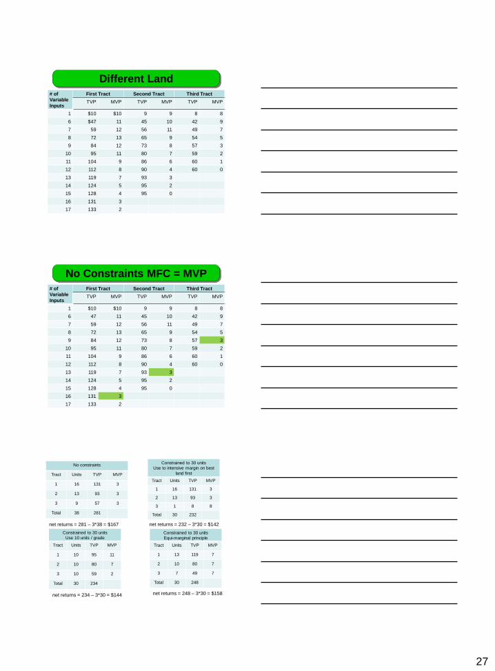
Different Land
# of
Variable
Inputs
First Tract Second Tract Third Tract
TVP MVP TVP MVP TVP MVP
1 $10 $10 9 9 8 8
6 $47 11 45 10 42 9
7 59 12 56 11 49 7
8 72 13 65 9 54 5
9 84 12 73 8 57 3
10 95 11 80 7 59 2
11 104 9 86 6 60 1
12 112 8 90 4 60 0
13 119 7 93 3
14 124 5 95 2
15 128 4 95 0
16 131 3
17 133 2
No Constraints MFC = MVP
# of
Variable
Inputs
First Tract Second Tract Third Tract
TVP MVP TVP MVP TVP MVP
1 $10 $10 9 9 8 8
6 47 11 45 10 42 9
7 59 12 56 11 49 7
8 72 13 65 9 54 5
9 84 12 73 8 57 3
10 95 11 80 7 59 2
11 104 9 86 6 60 1
12 112 8 90 4 60 0
13 119 7 93 3
14 124 5 95 2
15 128 4 95 0
16 131 3
17 133 2
No constraints
Tract Units TVP MVP
1 16 131 3
2 13 93 3
3 9 57 3
Total 38 281
Constrained to 30 units
Use to intensive margin on best
land first
Tract Units TVP MVP
1 16 131 3
2 13 93 3
3 1 8 8
Total 30 232
Constrained to 30 units
Use 10 units / grade
Tract Units TVP MVP
1 10 95 11
2 10 80 7
3 10 59 2
Total 30 234
Constrained to 30 units
Equi-marginal principle
Tract Units TVP MVP
1 13 119 7
2 10 80 7
3 7 49 7
Total 30 248
net returns = 281 – 3*38 = $167 net returns = 232 – 3*30 = $142
net returns = 234 – 3*30 = $144 net returns = 248 – 3*30 = $158
28
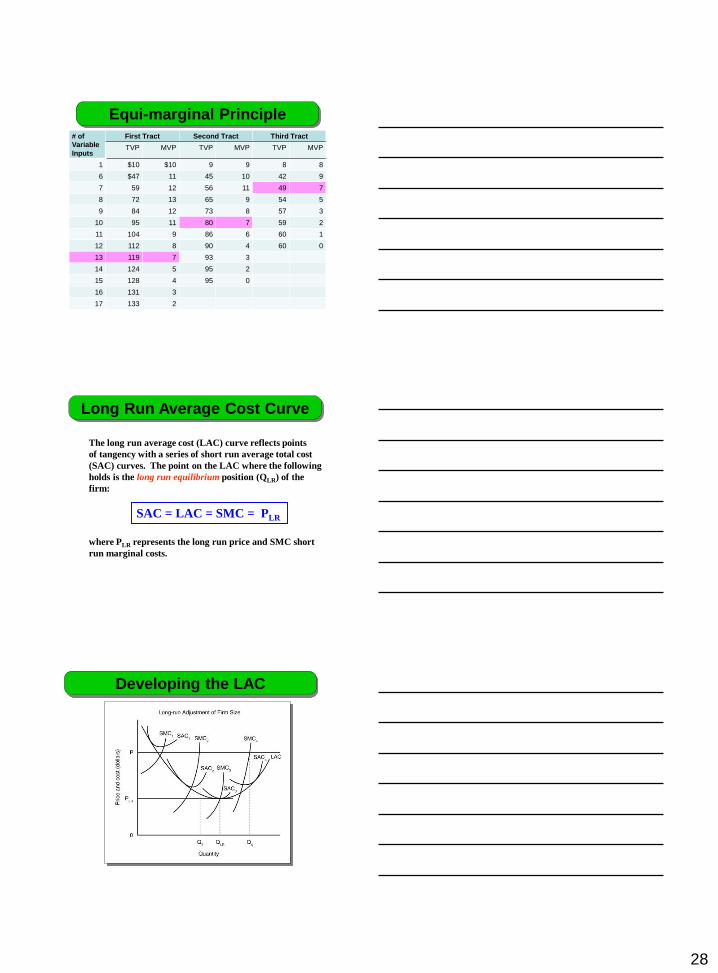
Equi-marginal Principle
# of
Variable
Inputs
First Tract Second Tract Third Tract
TVP MVP TVP MVP TVP MVP
1 $10 $10 9 9 8 8
6 $47 11 45 10 42 9
7 59 12 56 11 49 7
8 72 13 65 9 54 5
9 84 12 73 8 57 3
10 95 11 80 7 59 2
11 104 9 86 6 60 1
12 112 8 90 4 60 0
13 119 7 93 3
14 124 5 95 2
15 128 4 95 0
16 131 3
17 133 2
The long run average cost (LAC) curve reflects points
of tangency with a series of short run average total cost
(SAC) curves. The point on the LAC where the following
holds is the long run equilibrium position (QLR) of the
firm:
SAC = LAC = SMC = PLR
where PLR represents the long run price and SMC short
run marginal costs.
Long Run Average Cost Curve
Developing the LAC

29
• Increasing returns to size – increase in output is
more than proportional increase in input use
– LAC is decreasing when firm is expanded
• Decreasing returns to size - increase in output is
less than proportional increase in input use
– LAC is increasing when firm is expanded
• Constant returns to size - increase in output is
equal to the proportional increase in input use
– LAC is horizontal when firm is expanded
Economies of Size
Returns to Size
DecreasingIncreasing
Constant
What can we say about the four
firms in this graph?

30
Q3
WHY?
Size 1 would lose
money at price P
Q3
Firm size 2, 3 and 4
would earn a profit
at price P….
WHY?
Q3
Firm #2’s profit would
be the area shown
below…
31
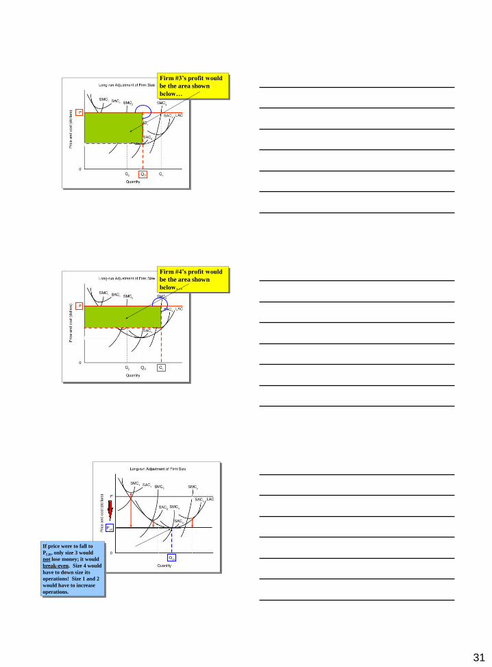
Q3
Firm #3’s profit would
be the area shown
below…
Q3
Firm #4’s profit would
be the area shown
below…
If price were to fall to
PLR, only size 3 would
not lose money; it would
break-even. Size 4 would
have to down size its
operations! Size 1 and 2
would have to increase
operations.