Embed Size (px)
Citation preview

Conduction Heat Transfer
Reading Problems10-1→ 10-6 10-20, 10-35, 10-49, 10-54, 10-59, 10-69,
10-71, 10-92, 10-126, 10-143, 10-157, 10-16211-1→ 11-2 11-14, 11-17, 11-36, 11-41, 11-46, 11-97, 11-104
General Heat ConductionFrom a 1st law energy balance:
∂E
∂t= Qx − Qx+∆x
If the volume to the element is given asV = A ·∆x, then the mass of the element is
m = ρ ·A ·∆xx=0
xx
x+ xD
x=Linsulated
Qx
Qx+ xD
A
The energy term (KE = PE = 0) is
E = m · u = (ρ ·A ·∆x) · u
For an incompressible substance the internal energy is du = C dT and we can write
∂E
∂t= ρCA∆x
∂T
∂t
Heat flow along the x−direction is a product of the temperature difference.
Qx =kA
∆x(Tx − Tx+∆x)
where k is the thermal conductivity of the material. In the limit as ∆x→ 0
Qx = −kA∂T
∂x
This is Fourier’s law of heat conduction. The −ve in front of k guarantees that we adhere to the2nd law and that heat always flows in the direction of lower temperature.
1

We can write the heat flow rate across the differential length, ∆x as a truncated Taylor seriesexpansion as follows
Qx+∆x = Qx +∂Qx
∂x∆x
when combined with Fourier’s equation gives
Qx+∆x = −kA∂T
∂x︸ ︷︷ ︸Qx
−∂
∂x
(kA
∂T
∂x
)∆x
Noting that
Qx − Qx+∆x =∂E
∂t= ρCA∆x
∂T
∂t
By removing the common factor of A∆x we can then write the general 1-D conduction equationas
∂
∂x
(k∂T
∂x
)︸ ︷︷ ︸
longitudinalconduction
= ρC∂T
∂t︸ ︷︷ ︸thermalinertia
↙ ↘
Steady Conduction Transient Conduction
•∂T
∂t→ 0
• properties are constant
• temperature varies in a linear manner
• heat flow rate defined by Fourier’sequation
• resistance to heat flow: R =∆T
Q
• properties are constant
• therefore∂2T
∂x2=ρC
k
∂T
∂t=
1
α
∂T
∂t
where thermal diffusivity is defined as
α =k
ρC
• exact solution is complicated
• partial differential equation can besolved using approximate or graphicalmethods
2

Steady Heat Conduction
Thermal Resistance Networks
Thermal circuits based on heat flow rate, Q, temperature difference, ∆T and thermal resistance,R, enable analysis of complex systems.
Thermal Resistance
The thermal resistance to heat flow (◦C/W ) can be constructed for all heat transfer mechanisms,including conduction, convection, and radiation as well as contact resistance and spreading resis-tance.
R - film resistancef
R - fin resistancefin
R - base resistanceb
R - spreading resistancesR - contact resistancec
Tsource
Tsink
Conduction: Rcond =L
kA
Convection: Rconv =1
hA
Radiation: Rrad =1
hradA−→ hrad = εσ(T 2
s + T 2surr)(Ts + Tsurr)
Contact: Rc =1
hcA−→ hc see Table 10-2
Cartesian Systems
Resistances in Series
The heat transfer across the fluid/solid interface is based on Newton’s law of cooling
Q = hA(Tin − Tout) =Tin − ToutRconv
where Rconv =1
hA
3

The heat flow through a solid material of conductivity, k is
Q =kA
L(Tin − Tout) =
Tin − ToutRcond
where Rcond =L
kA
By summing the temperature drop acrosseach section, we can write:
Q R1 = (T∞1 − T1)
Q R2 = (T1 − T2)
Q R3 = (T2 − T3)
Q R4 = (T3 − T∞2)
Q
(4∑i=1
Ri
)= (T∞1 − T∞2)
The total heat flow across the system can be written as
Q =T∞1 − T∞2
Rtotal
where Rtotal =4∑i=1
Ri
4

Resistances in Parallel
For systems of parallel flow paths asshown above, we can use the 1st lawto preserve the total energy
Q = Q1 + Q2
where we can write
L
T1
T2
R1
R2
R3
k1
k2
k3
Q1 =T1 − T2
R1
R1 =L
k1A1
Q2 =T1 − T2
R2
R2 =L
k2A2
Q =∑Qi = (T1 − T2)
(∑ 1
Ri
)where
1
Rtotal
=∑ 1
Ri
= UA
In general, for parallel networks we can use a parallel resistor network as follows:
T1
T1
T2 T
2
R1
RtotalR
2
R3
=
1
Rtotal
=1
R1
+1
R2
+1
R3
+ · · ·
and
Q =T1 − T2
Rtotal
5

Thermal Contact Resistance
• real surfaces have microscopic roughness,leading to non-perfect contacts where
– 1 - 4% of the surface area is in solid-solidcontact, the remainder consists of air gaps
• the total heat flow rate can bewritten as
Qtotal = hcA∆Tinterface
where:
hc = thermal contact conductanceA = apparent or projected area of the contact∆Tinterface = average temperature drop across the interface
The conductance, hc and the contact resistance,Rc can be written as
hcA =Qtotal
∆Tinterface=
1
Rc
Table 10-2 can be used to obtain some representative values for contact conductance
Table 10-2: Contact Conductances
6

Cylindrical Systems
L
r1
r2
Qr
T1
T2
A=2 rLp
k
r
Steady, 1D heat flow from T1 to T2
in a cylindrical system occurs in a ra-dial direction where the lines of con-stant temperature (isotherms) are con-centric circles, as shown by the dottedline and T = T (r).Performing a 1st law energy balanceon a control mass from the annularring of the cylindrical cylinder gives:
Qr =T1 − T2(
ln(r2/r1)
2πkL
) where R =
(ln(r2/r1)
2πkL
)
Composite Cylinders
Then the total resistance can be written as
Rtotal = R1 +R2 +R3 +R4
=1
h1A1
+ln(r2/r1)
2πk2L+
ln(r3/r2)
2πk3L+
1
h4A4
7
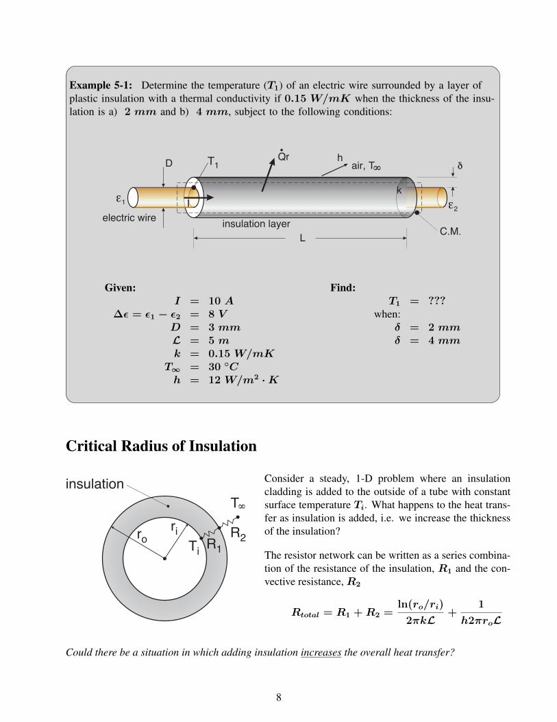
Example 5-1: Determine the temperature (T1) of an electric wire surrounded by a layer ofplastic insulation with a thermal conductivity if 0.15 W/mK when the thickness of the insu-lation is a) 2 mm and b) 4 mm, subject to the following conditions:
Given: Find:I = 10 A T1 = ???
∆ε = ε1 − ε2 = 8 V when:D = 3 mm δ = 2 mmL = 5 m δ = 4 mmk = 0.15 W/mK
T∞ = 30 ◦Ch = 12 W/m2 ·K
Critical Radius of Insulation
Consider a steady, 1-D problem where an insulationcladding is added to the outside of a tube with constantsurface temperature Ti. What happens to the heat trans-fer as insulation is added, i.e. we increase the thicknessof the insulation?
The resistor network can be written as a series combina-tion of the resistance of the insulation, R1 and the con-vective resistance,R2
Rtotal = R1 +R2 =ln(ro/ri)
2πkL+
1
h2πroL
Could there be a situation in which adding insulation increases the overall heat transfer?
8

dRtotal
dro=
1
2πkroL−
1
h2πr2oL
= 0 ⇒ rcr,cyl =k
h[m]
resis
tan
ce
Rtotal
R1
added insulation
lowers resistance
added insulation
increases resistance
Rbare
R2
ri
ror
c
There is always a value of rcr,cal, but there is a minimum in heat transfer only if rcr,cal > ri
Spherical Systems
For steady, 1D heat flow in spherical geometries we can writethe heat transfer in the radial direction as
Q =4πkriro
(r0 − ri)(Ti − To) =
(Ti − To)R
where: R =ro − ri4πkriro
ri
ro
Ti
To
The critical radius of insulation for a spherical shell is given as
rcr,sphere =2k
h[m]
9

Heat Transfer from Finned SurfacesWe can establish a 1st law balance over the thin slice ofthe fin between x and x+ ∆x such that
Qx − Qx+∆x − P∆x︸ ︷︷ ︸Asurface
h(T − T∞) = 0
From Fourier’s law we know
Qx − Qx+∆x = kAc
d2T
dx2∆x
Therefore the conduction equation for a fin with constantcross section is
kAc
d2T
∂x2︸ ︷︷ ︸longitudinalconduction
−hP (T − T∞)︸ ︷︷ ︸lateral
convection
= 0
Let the temperature difference between the fin and the surroundings (temperature excess) beθ = T (x)− T∞ which allows the 1-D fin equation to be written as
d2θ
dx2−m2θ = 0 where m =
(hP
kAc
)1/2
The solution to the differential equation for θ is
θ(x) = C1 sinh(mx) + C2 cosh(mx) [≡ θ(x) = C1emx + C2e
−mx]
Potential boundary conditions include:
Base: → @x = 0 θ = θbTip: → @x = L θ = θL [T -specified tip]
θ =dθ
dx
∣∣∣∣∣x=L
= 0 [adiabatic (insulated) tip]
θ → 0 [infinitely long fin]
Substituting the boundary conditions to find the constants of integration, the temperature distribu-tion and fin heat transfer rate can be determined as follows:
Case 1: Prescribed temperature (θ@ x+L = θL)
θ(x)
θb=
(θL/θb) sinhmx+ sinhm(L− x)
sinhmL
10

Qb = M(coshmL− θL/θb)
sinhmL
Case 2: Adiabatic tip(dθ
dx
∣∣∣∣∣x=L
= 0
)
θ(x)
θb=
coshm(L− x)
coshmLQb = M tanhmL
Case 3: Infinitely long fin (θ → 0)
θ(x)
θb= e−mx Qb = M
where
m =√hP/(kAc)
M =√hPkAc θb
θb = Tb − T∞
Fin Efficiency and Effectiveness
The dimensionless parameter that compares the actual heat transfer from the fin to the ideal heattransfer from the fin is the fin efficiency
η =actual heat transfer rate
maximum heat transfer rate whenthe entire fin is at Tb
=Qb
hPLθb
If the fin has a constant cross section then
η =tanh(mL)
mL
An alternative figure of merit is the fin effectiveness given as
εfin =total fin heat transfer
the heat transfer that would haveoccurred through the base area
in the absence of the fin
=Qb
hAcθb
11

How to Determine the Appropriate Fin Length
• theoretically an infinitely long fin willdissipate the most heat
• but practically, an extra long fin is in-efficient given the exponential temper-ature decay over the length of the fin
• so what is a realistic fin length in orderto optimize performance and cost
If we determine the ratio of heat flow for afin with an insulated tip (Case 2) versus aninfinitely long fin (Case 3) we can assess therelative performance of a conventional fin
QCase 2
QCase 3
=M tanhmL
M= tanhmL
High
heat
transfer
Low
heat
transfer
No
heat
transfer
T
T
T
x
Tb
L
T = highT= low
T = 0
h, T
T(x)
0
Transient Heat ConductionPerforming a 1st law energy balance on a planewall gives
Qcond =TH − TsL/(k ·A)
= Qconv =Ts − T∞1/(h ·A)
where the Biot number can be obtained as follows:
TH − TsTs − T∞
=L/(k ·A)
1/(h ·A)=
internal resistance to H.T.external resistance to H.T.
=hL
k= Bi
Rint << Rext: the Biot number is small and we can conclude
TH − Ts << Ts − T∞ and in the limit TH ≈ Ts
Rext << Rint: the Biot number is large and we can conclude
Ts − T∞ << TH − Ts and in the limit Ts ≈ T∞
12

Transient Conduction Analysis• if the internal temperature of a body remains relatively constant with respect to time
– can be treated as a lumped system analysis
– heat transfer is a function of time only, T = T (t)
T T T T
T(t)
L LL L
tt
x x
T(x,0) = Ti
T(x,t)
Bi 0.1≤ Bi > 0.1
Bi ≤ 0.1: temperature profile is not a function of positiontemperature profile only changes with respect to time→ T = T (t)use lumped system analysis
Bi > 0.1: temperature profile changes with respect to time and position→ T = T (x, t)use approximate analytical or graphical solutions (Heisler charts)
Lumped System Analysis
At t > 0, T = T (x, y, z, t), however, whenBi ≤ 0.1 then we can assume T ≈ T (t).
13

Performing a 1st law energy balance on the control volume shown below
dEC.M.
dt= Ein − Eout + Eg↗0
If we assume PE andKE to be negligible then
dU
dt= −Q ⇐
dU
dt< 0 implies U is decreasing
For an incompressible substance specific heat is constant and we can write
mC︸ ︷︷ ︸≡Cth
dT
dt= − Ah︸︷︷︸
1/Rth
(T − T∞)
where Cth = lumped capacitance
CthdT
dt= −
1
Rth
(T − T∞)
We can integrate and apply the initial condition, T = Ti @t = 0 to obtain
T (t)− T∞Ti − T∞
= e−t/(Rth·Cth) = e−t/τ = e−bt
where
1
b= τ
= Rth · Cth
= thermal time constant
=mC
Ah=ρV C
Ah
The total heat transferred over the time period 0→ t∗ is
Qtotal = mC(Ti − T∞)[1− e−t∗/τ ]
14

Example 5-2: Determine the time it takes a fuse to melt if a current of 3 A suddenly flowsthrough the fuse subject to the following conditions:
Given:D = 0.1 mm Tmelt = 900 ◦C k = 20 W/mK
L = 10 mm T∞ = 30 ◦C α = 5× 10⁻⁵ m2/s ≡ k/ρCp
Assume:
• constant resistance R = 0.2 ohms
• the overall heat transfer coefficient is h = hconv + hrad = 10 W/m2K
• neglect any conduction losses to the fuse support
15

Approximate Analytical and Graphical Solutions (Heisler Charts)IfBi > 0.1
• need to solve the partial differential equation for temperature
• leads to an infinite series solution⇒ difficult to obtain a solution(see pp. 481 - 483 for exact solution by separation of variables)
We must find a solution to the PDE
∂2T
∂x2=
1
α
∂T
∂t⇒
T (x, t)− T∞Ti − T∞
=∞∑
n=1,3,5...
Ane
(−λn
L
)2
αt
cos
(λnx
L
)
By using dimensionless groups, we can reduce the temperature dependence to 3 dimensionlessparameters
Dimensionless Group Formulation
temperature θ(x, t) =T (x, t)− T∞Ti − T∞
position X = x/L
heat transfer Bi = hL/k Biot number
time Fo = αt/L2 Fourier number
note: Cengel uses τ instead of Fo.
Now we can write
θ(x, t) = f(X,Bi, Fo)
The characteristic length for the Biot number is
slab L = Lcylinder L = rosphere L = ro
contrast this versus the characteristic length for the lumped system analysis.
16

With this, two approaches are possible
1. use the first term of the infinite series solution. This method is only valid for Fo > 0.2
2. use the Heisler charts for each geometry as shown in Figs. 11-15, 11-16 and 11-17
First term solution: Fo > 0.2→ error about 2% max.
Plane Wall: θwall(x, t) =T (x, t)− T∞Ti − T∞
= A1e−λ2
1Fo cos(λ1x/L)
Cylinder: θcyl(r, t) =T (r, t)− T∞Ti − T∞
= A1e−λ2
1Fo J0(λ1r/ro)
Sphere: θsph(r, t) =T (r, t)− T∞Ti − T∞
= A1e−λ2
1Fosin(λ1r/ro)
λ1r/ro
λ1, A1 can be determined from Table 11-2 based on the calculated value of the Biot number (willlikely require some interpolation). The Bessel function, J0 can be calculated using Table 11-3.
Using Heisler Charts
• find T0 at the center for a given time (Table 11-15 a, Table 11-16 a or Table 11-17 a)
• find T at other locations at the same time (Table 11-15 b, Table 11-16 b or Table 11-17 b)
• findQtot up to time t (Table 11-15 c, Table 11-16 c or Table 11-17 c)
Example 5-3: An aluminum plate made of Al 2024-T6 with a thickness of 0.15 m isinitially at a temperature of 300 K. It is then placed in a furnace at 800 K with aconvection coefficient of 500 W/m2K.
Find: i) the time (s) for the plate midplane to reach 700 Kii) the surface temperature at this condition. Use both the Heisler charts
and the approximate analytical, first term solution.
17