Confined water effects on the viscous flow around a tanker

International Shipbuilding Progress 60 (2013) 309–343 309DOI 10.3233/ISP-130101IOS Press

Confined water effects on the viscous flow arounda tanker with propeller and rudder

L. Zou ∗ and L. LarssonChalmers University of Technology, Gothenburg, Sweden

A ship travelling in canals or narrow channels may encounter hydrodynamic forces and momentscaused by a nearby side bank. Since most canals are shallow the effect of the bottom can also be con-siderable. Knowledge of these effects is crucial for safe navigation. The present paper introduces a studyin the framework of a project applying Computational Fluid Dynamics (CFD) in the prediction of con-fined water effects. Using a steady state Reynolds Averaged Navier–Stokes solver, this study investigatesthe shallow-water and bank effects on a tanker moving straight ahead at low speed in a canal characterizedby surface piercing banks. The tanker is fitted with a rudder and a propeller at a zero propeller rate and atself-propulsion. In the systematic computations, a series of cases are considered with varying water depthand ship-to-bank distance, as well as different canal configurations. In the computations, the double modelapproximation is adopted to simulate the flat free surface. The non-rotating propeller is treated as an ap-pendage composed of shaft and blades, while the operating propeller is approximated by body forces,simulated by a lifting line potential flow model. Validation of forces and moments against experimentaldata has been performed in previous studies. The emphasis of the present paper is placed on the effectson the flow field and the physical explanation of these effects.

Keywords: Confined water effects, computational fluid dynamics, hydrodynamic forces and moments,verification and validation, flow field analysis

1. Introduction

As long as a ship is surrounded by the water flow, the forces and moments actingon it are affected by the presence of solid boundaries of the flow field, such as ashallow seabed below the hull, or a side bank in the vicinity of the hull. The term“shallow-water effects” in this case refers to the influence from the seabed, and “bankeffects” to the influence from the side bank. In a canal, often both effects are signif-icant. The influence on flow and hydrodynamic quantities then results in significantchanges in ship motion, and leads to problems in ship maneuvering and navigation.The explanation of confined water effects is that when the distance between the hulland the seabed or the side bank is narrowed, the flow is accelerated and the pressureis accordingly decreased, which induces a variation in the hydrodynamic character-istics. The produced hydrodynamic forces, especially in extremely shallow canals,

*Corresponding author. E-mail: [email protected].

0020-868X/13/$27.50 © 2013 – IOS Press and the authors. All rights reserved

310 L. Zou and L. Larsson / Confined water effects on the viscous flow

may considerably affect the maneuvering performance of the ship, making it diffi-cult to steer. The ship may collide with the side bank and/or run aground due to theso-called “squat” phenomenon. From this point of view, confined water effects areextremely important for ship navigation. In the past few decades, many investiga-tions on confined water effects have been carried out, both experimentally and nu-merically. A notable event was the International Conference on Ship Maneuvering inShallow and Confined Water: Bank Effects [13], at which the participants expressedbroad concern about this problem and presented many interesting papers.

However, historical investigations of bank effects have mostly relied on experi-mental tools, such as model tests and empirical or semi-empirical formulae, whichnormally treat the bank effect as a function involving hull-bank distance, water depth,ship speed, hull form, bank geometry, propeller performance, etc. During the 1970s,Norrbin at SSPA, Sweden, carried out experimental research and then, based on theexperiments, proposed empirical formulae to estimate the hydrodynamic forces forflooded [25], vertical [24] and sloping [24] banks. Li et al. [19] continued Norrbin’sinvestigations and tested the bank effect in extreme conditions for three different hullforms (tanker, ferry and catamaran). The influence of ship speed, propeller loadingand bank inclination was evaluated. Ch’ng et al. [3] conducted a series of model testsand developed an empirical formula to estimate the bank-induced sway force andyaw moment for a ship handling simulator. In recent years, comprehensive modeltests in a towing tank have been carried out at Flanders Hydraulics Research (FHR),Belgium, to build up mathematical models for bank-effect investigations and to pro-vide data for computation validation. Vantorre et al. [30] discussed the influence ofwater depth, lateral distance, forward speed and propulsion on the hydrodynamicforces and moments based on a systematic captive model test program for three shipmodels moving along a vertical surface-piercing bank. They also proposed empiri-cal formulae for the prediction of ship-bank interaction forces. From extensive tests,Lataire et al. [15] developed a mathematical model for the estimation of the hydrody-namic forces, moments and motions taking into consideration ship speed, propulsionand ship/bank geometry.

Although empirical formulae are widely used for bank-effect predictions, theyhave their shortcomings due to the approximation. They should only be used forcases within a given range of hull forms and conditions. Otherwise, the predictionis barely reliable. To establish a mathematical model, a significant number of sys-tematic and expensive model tests is always required. However, the most importantweakness of most experiments and empirical relations is their inability to providedetailed information on the flow field, which can explain the flow mechanism be-hind the bank effects. In view of this, researchers resort to using numerical methodsto deal with the phenomena of bank effects. Among existing numerical methods, thepotential flow method is the most common one. For instance, the slender-body theorydeveloped by Tuck [28,29] is still widely used for ship squat prediction in confinedwaters [10]. Other examples of the potential flow method are available in the stud-ies by, e.g., Newman [23], Miao et al. [22] and Lee et al. [16]. All these references

L. Zou and L. Larsson / Confined water effects on the viscous flow 311

only give quantitative predictions of the forces and moments on the hull travellingin canal or channel, but without any information on the flow field. Using a viscousflow method, Lo et al. [20] studied the bank effect on a container ship model us-ing CFD software based on the Navier–Stokes equations. The effect of vessel speedand distance to bank on the magnitude and temporal variation of the yaw angle andsway force were reported. Some details of the predicted flow field are available inthis work. Wang et al. [31] studied the vertical bank effects using a Reynolds Av-eraged Navier–Stokes (RANS) method. This study predicted viscous hydrodynamicforces on a Series 60 hull at varying water depth to draught ratios and ship-to-bankdistances, as well as simulated the pressure distribution on the hull.

In an ongoing project at Chalmers a CFD method is used in the prediction of con-fined water effects, such as shallow-water effects, bank effects and the ship-to-shipinteraction. Regarding the investigation of shallow-water and bank effects, valida-tion of viscous forces and moments against experimental data has been presented inthree reports: Zou et al. [34,35] and Zou [33]. In these reports, forces and momentspredicted by a RANS solver have shown reasonable correspondence with the mea-surements in terms of the variation of water depth and ship-bank distance. To furtherextend the investigation of confined-water effects in [34], the present paper aims atexplaining the effects on the flow field and the physical explanation of these effects.

2. Geometries and test conditions

The test cases for systematic computations were determined from straight-linecaptive model tests for a second variant of the KRISO Very Large Crude-oil Carrier(KVLCC2).

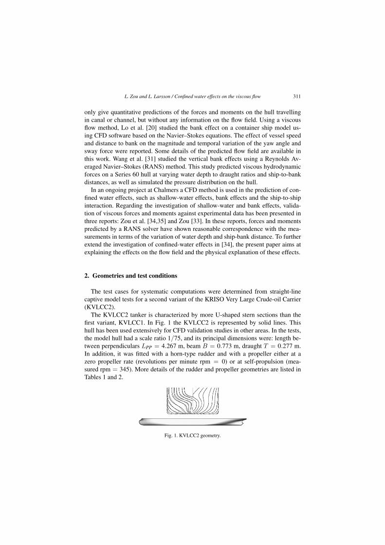
The KVLCC2 tanker is characterized by more U-shaped stern sections than thefirst variant, KVLCC1. In Fig. 1 the KVLCC2 is represented by solid lines. Thishull has been used extensively for CFD validation studies in other areas. In the tests,the model hull had a scale ratio 1/75, and its principal dimensions were: length be-tween perpendiculars LPP = 4.267 m, beam B = 0.773 m, draught T = 0.277 m.In addition, it was fitted with a horn-type rudder and with a propeller either at azero propeller rate (revolutions per minute rpm = 0) or at self-propulsion (mea-sured rpm = 345). More details of the rudder and propeller geometries are listed inTables 1 and 2.

Fig. 1. KVLCC2 geometry.


Table 1

Rudder data (model scale)

Type Horn

Section NACA0018

Wetted surface area (m2) 0.0486

Lateral area (m2) 0.0243

Table 2

Propeller data (model scale)

Name MOERI KP458

Type Fixed pitch

No. of propeller Single

No. of blades 4

Diameter DR (m) 0.131

Pitch ratio PR/DR(0.7R) 0.721

Expanded area ratio AE/A0 0.431

Rotation Right hand

Hub ratio 0.155

Skew (◦) 21.150

Rake (◦) 0.000

Fig. 2. Geometry of the towing tank built with two canals. (Colors are visible in the online version of thearticle; http://dx.doi.org/10.3233/ISP-130101.)

The captive model tests were made in two canals (A and B), built up in the shal-low water towing tank at the Flanders Hydraulics Research (FHR) in co-operationwith the Maritime Technology Division of Ghent University, Belgium. The KVLCC2tanker was tested at a speed U0 = 0.356 m/s (6 knots full scale) along one side ofthe canals, i.e. it moved close to the vertical bank (Canal A) and the bank with slope1 : 1 (Canal B) at its starboard side. A brief illustration of the Canal A and Canal Bconfigurations shaped by surface-piercing banks is given in Fig. 2 (the arrow indi-cates the direction of motion), and cross-section profiles of the two canals are furtherpresented in Fig. 3. The tests in Canal A and Canal B were conducted at three differ-ent under keel clearances (UKC), namely 50%, 35% and 10% of the draught (waterdepth to ship draught ratio h/T = 1.50, 1.35, 1.10), and at four different lateralpositions (ship-bank distance) chosen in combination with the water depth [34]. The


Fig. 3. Cross-sections of Canal A (top) and Canal B (bottom), seen in the direction of motion.

Table 3

Matrix of test conditions

yB Canal A

1.180 1.316 1.961 2.431

Canal B

h/T 0.758 0.909 1.632 2.173

1.50 (UKC = 50%T ) 0

1.35 (UKC = 35%T ) 0/345 0/345 0/345 0/345

1.10 (UKC = 10%T ) 0

non-dimensional ship-bank distance yB is defined as below, following the proposalsby e.g., Ch’ng et al. [3]:

1yB

=B

2

(1yP

+1yS

), (1)

yP , yS represents the respective distance from the ship center-plane to the toe ofthe bank at the port/starboard side. This description thus takes two side banks intoconsideration, due to the non-uniform bank geometries and canal configurations.

A subset of the test conditions was selected for the validation including varia-tions of the water depth and the ship-bank distance. Details are shown in Table 3.“0” represent the test cases with only a non-rotating propeller (rpm = 0), while“0/345” indicate cases with the propeller both at a zero rpm and at self-propulsion(rpm = 345). As can be seen, there are six water depth and ship-bank distance com-binations in each canal, some of which rather extreme, which put the computationaltools to a severe test. No waves are considered, since the tanker moves at a low speed(U0 = 0.356 m/s). The corresponding Froude number is Fr = U0/

√gLPP = 0.055

(largest depth Froude number Frh = U0/√gh = 0.206) and the Reynolds number is

Re = U0 · LPP/ν = 1.513 × 106 (g is the acceleration of gravity and ν is the kine-matic viscosity of water). As a result, the double model approximation is adoptedand no sinkage and trim is considered.


3. Computational method

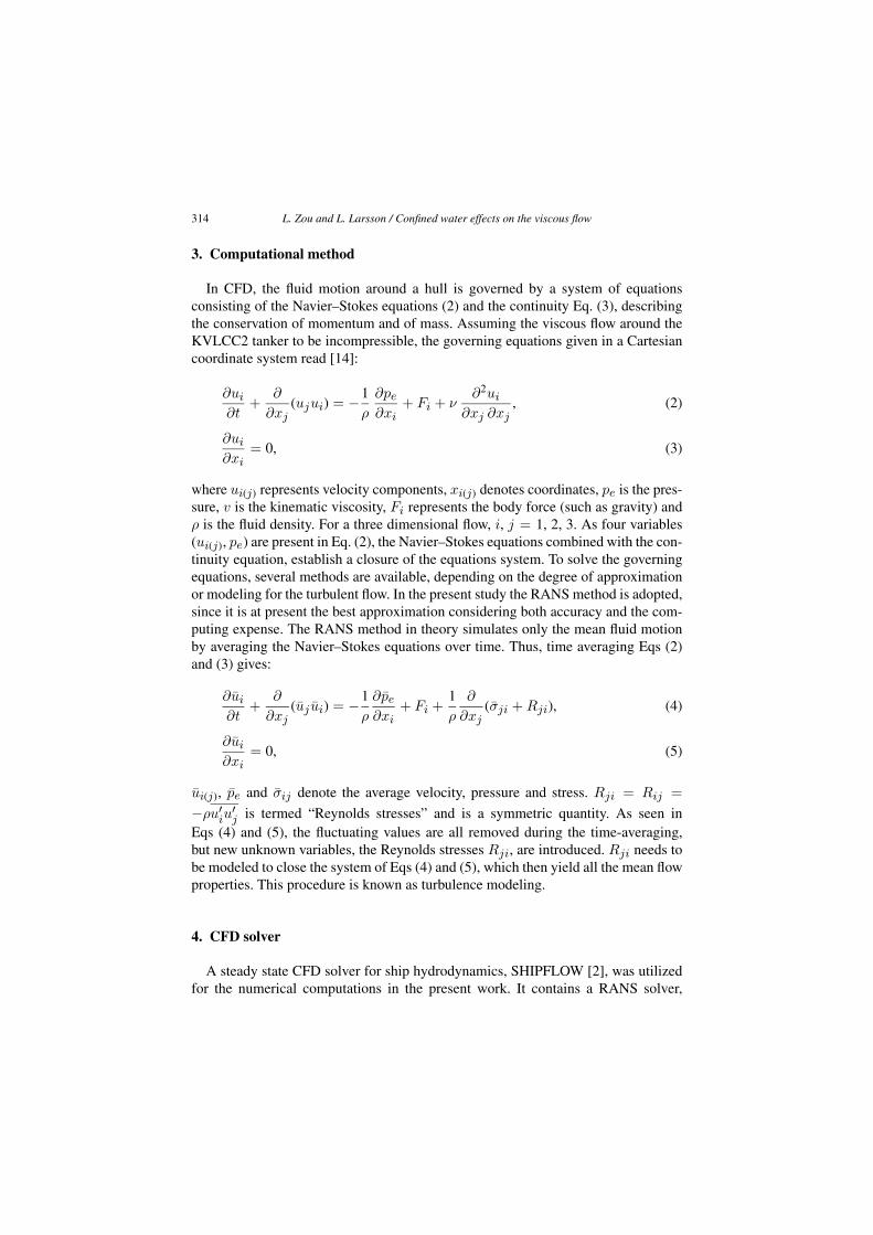
In CFD, the fluid motion around a hull is governed by a system of equationsconsisting of the Navier–Stokes equations (2) and the continuity Eq. (3), describingthe conservation of momentum and of mass. Assuming the viscous flow around theKVLCC2 tanker to be incompressible, the governing equations given in a Cartesiancoordinate system read [14]:

∂ui∂t

+∂

∂xj(ujui) = −1

ρ

∂pe∂xi

+ Fi + ν∂2ui

∂xj ∂xj, (2)

∂ui∂xi

= 0, (3)

where ui(j) represents velocity components, xi(j) denotes coordinates, pe is the pres-sure, v is the kinematic viscosity, Fi represents the body force (such as gravity) andρ is the fluid density. For a three dimensional flow, i, j = 1, 2, 3. As four variables(ui(j), pe) are present in Eq. (2), the Navier–Stokes equations combined with the con-tinuity equation, establish a closure of the equations system. To solve the governingequations, several methods are available, depending on the degree of approximationor modeling for the turbulent flow. In the present study the RANS method is adopted,since it is at present the best approximation considering both accuracy and the com-puting expense. The RANS method in theory simulates only the mean fluid motionby averaging the Navier–Stokes equations over time. Thus, time averaging Eqs (2)and (3) gives:

∂ui∂t

+∂

∂xj(uj ui) = −1

ρ

∂pe∂xi

+ Fi +1ρ

∂

∂xj(σji +Rji), (4)

∂ui∂xi

= 0, (5)

ui(j), pe and σij denote the average velocity, pressure and stress. Rji = Rij =

−ρu′iu′j is termed “Reynolds stresses” and is a symmetric quantity. As seen in

Eqs (4) and (5), the fluctuating values are all removed during the time-averaging,but new unknown variables, the Reynolds stresses Rji, are introduced. Rji needs tobe modeled to close the system of Eqs (4) and (5), which then yield all the mean flowproperties. This procedure is known as turbulence modeling.

4. CFD solver

A steady state CFD solver for ship hydrodynamics, SHIPFLOW [2], was utilizedfor the numerical computations in the present work. It contains a RANS solver,


XCHAP, based on the finite volume method. In XCHAP, the discretization of con-vective terms is implemented by a Roe scheme [27] and for the diffusive fluxes cen-tral differences are applied. To approach second order accuracy, a flux correction isadopted [6]. An Alternating Direction Implicit scheme (ADI) is utilized to solve thediscrete equations. Two turbulence models are available in XCHAP: the Shear StressTransport k–ω model (k–ω SST model) [21] and the Explicit Algebraic Stress Model(EASM) [5,9]. As for the specified boundary conditions, the available options are:inflow, outflow, no-slip, slip and interior conditions. (a) Inflow condition: is normallysatisfied at an inlet plane of the computational domain to guarantee an undisturbedflow in front of a hull. In XCHAP it specifies a fixed velocity equal to the ship speedand estimated values of k and ω. The pressure gradient normal to the inlet plane is setto zero. (b) Outflow condition: describes zero normal gradients of velocity, k, ω andfixed pressure at a downstream outlet plane of the domain far behind a hull. (c) No-slip condition: simulates a solid wall boundary (e.g. a hull surface) by designatingzero value to velocity components, k, normal pressure gradient, and treating ω fol-lowing [12]. (d) Slip condition: specifies the normal velocity component and normalgradient of all other flow quantities (e.g. pressure) as zero. It simulates a symmetrycondition on flat boundaries. (e) Interior condition: describes the boundary data byinterpolation from another grid.

5. Computational setup

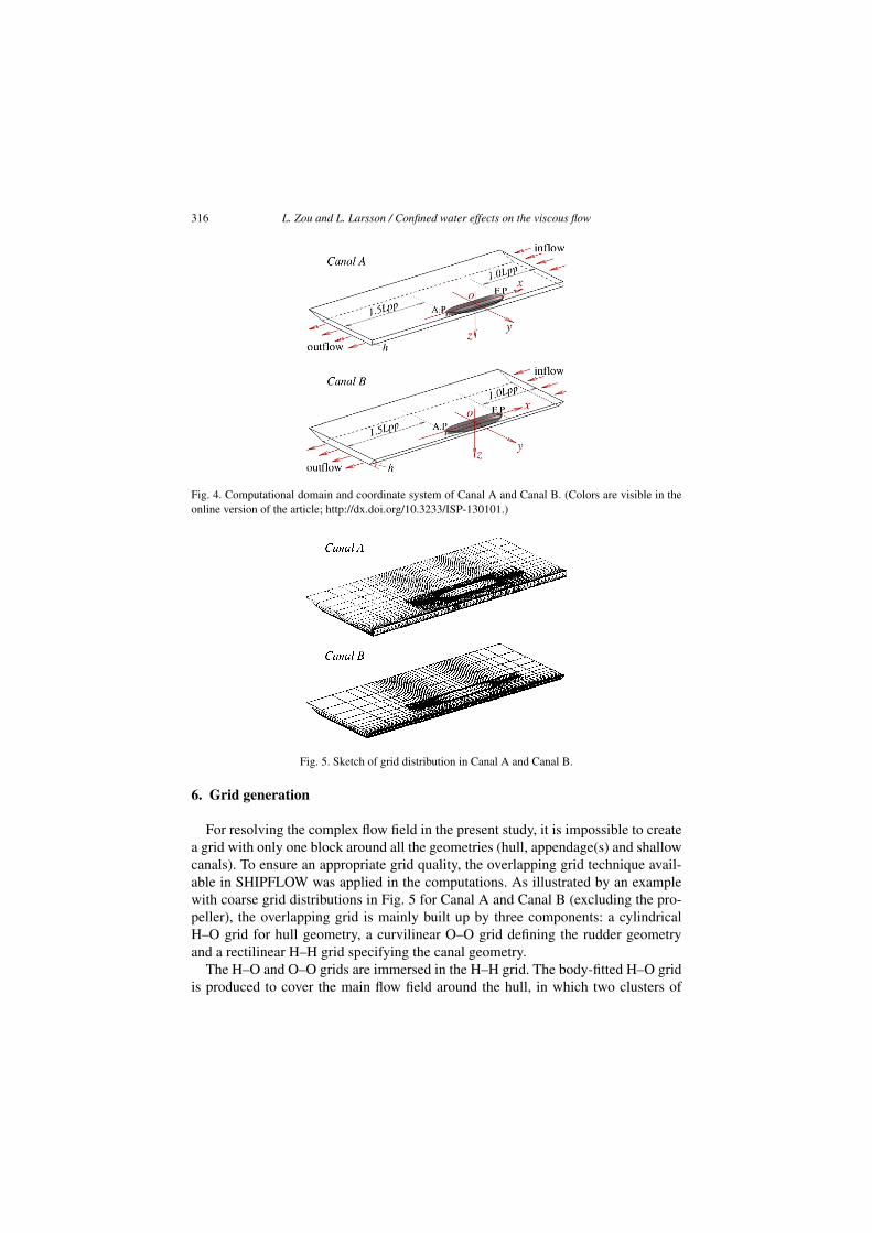
Due to the asymmetry of the bank geometry and so the flow field, the compu-tational domain has to cover the flow field around the whole hull in the canal.A schematic diagram indicating the coordinate system and the computational domainfor Canal A and Canal B is given in Fig. 4. As presented in the figure, the coordinatesystem is defined as a body-fixed and right-handed Cartesian system, with the ori-gin at the intersection of the flat free surface, the ship center-plane and the mid-shipsection. The axes x, y, z are directed towards the bow, to starboard and downwards,respectively.

The computational domain is made up by seven boundaries: inlet plane, outletplane, hull surface, flat free surface, seabed boundary, as well as two side banks.The inlet plane is located at 1.0LPP in front of the fore-perpendicular (F.P.) and theoutlet plane is at 1.5LPP behind the aft-perpendicular (A.P.). The flat free surface isconsidered at z = 0, while the seabed and the two side banks are placed at specificlocations as seen in Table 3. As to the adopted boundary conditions in the com-putations, the no-slip condition is satisfied on the hull surface (no wall function isintroduced and the non-dimensional wall distance y+ < 1.0 is employed instead);the inflow/outflow condition is set at the respective inlet/outlet boundary plane; theslip condition is set at the flat free surface (z = 0), the seabed and the side banks.


Fig. 4. Computational domain and coordinate system of Canal A and Canal B. (Colors are visible in theonline version of the article; http://dx.doi.org/10.3233/ISP-130101.)

Fig. 5. Sketch of grid distribution in Canal A and Canal B.

6. Grid generation

For resolving the complex flow field in the present study, it is impossible to createa grid with only one block around all the geometries (hull, appendage(s) and shallowcanals). To ensure an appropriate grid quality, the overlapping grid technique avail-able in SHIPFLOW was applied in the computations. As illustrated by an examplewith coarse grid distributions in Fig. 5 for Canal A and Canal B (excluding the pro-peller), the overlapping grid is mainly built up by three components: a cylindricalH–O grid for hull geometry, a curvilinear O–O grid defining the rudder geometryand a rectilinear H–H grid specifying the canal geometry.

The H–O and O–O grids are immersed in the H–H grid. The body-fitted H–O gridis produced to cover the main flow field around the hull, in which two clusters of


grid points are concentrated around the bow and stern regions so as to resolve theflow field more precisely. A small outer radius (0.2LPP) of the cylindrical grid isused for Canal A to save grid points and an even smaller radius (0.12LPP) of thecylindrical H–O grid is applied for Canal B. The body-fitted component O–O typegrid is generated internally to describe the rudder. Finally, a “box” of the rectilinearH–H grid is employed to take care of the remaining part of the domain within theinflow plane, outflow plane, seabed and side banks.

7. Experiences from a previous verification and validation study and aninvestigation of modeling error

Prior to the systematic computations, a preliminary verification and validation(V&V) study was performed [33] to assess the numerical error and to clarify themodeling error in the computations. This was accomplished through a grid conver-gence and formal validation study for the predicted forces and moments. In thissection, a brief description of the study and the results are introduced.

For the grid convergence study a representative test was set up, with its basic spec-ification comparable with that of the systematic computations. A KVLCC2 modeltanker (scale factor 1/45.714) moved slowly at U0 = 0.530 m/s (Fr = 0.064/Frh =0.237, Re = 3.697 × 106) in a shallow canal with vertical, surface piercing sidebanks. No appendage was attached to the tanker, but the condition was quite ex-treme: h/T = 1.12 and a non-dimensional ship-to-bank distance yB = 0.6B. Thecanal configuration is given in Fig. 6, indicating that the hull is moving close to thebank on the port side of the canal. Computational settings (coordinates system, do-main, grid generation, boundary conditions, etc.) in the grid convergence study werein accordance with the descriptions in the previous sections.

The estimation of numerical errors and uncertainties followed the proposal by Eçaet al. [7,8], see the Appendix. Six systematically refined grids were created with auniform grid refinement ratio r = 4

√2 to enable a curve fit by the Least Squares

Root method, so as to minimize the impact of scatter on the determination of gridconvergence. The grid convergence study was made for the non-dimensional longi-tudinal force (X ′), sway force (Y ′), roll moment (K ′) and yaw moment (N ′), whichare defined as follows:

X ′ = X/(0.5ρU2

0LPPT), Y ′ = Y/

(0.5ρU2

0LPPT),

K ′ = K/(0.5ρU2

0LPPT2), N ′ = N/

(0.5ρU2

0L2PPT

).

Fig. 6. Canal configuration in grid convergence study.


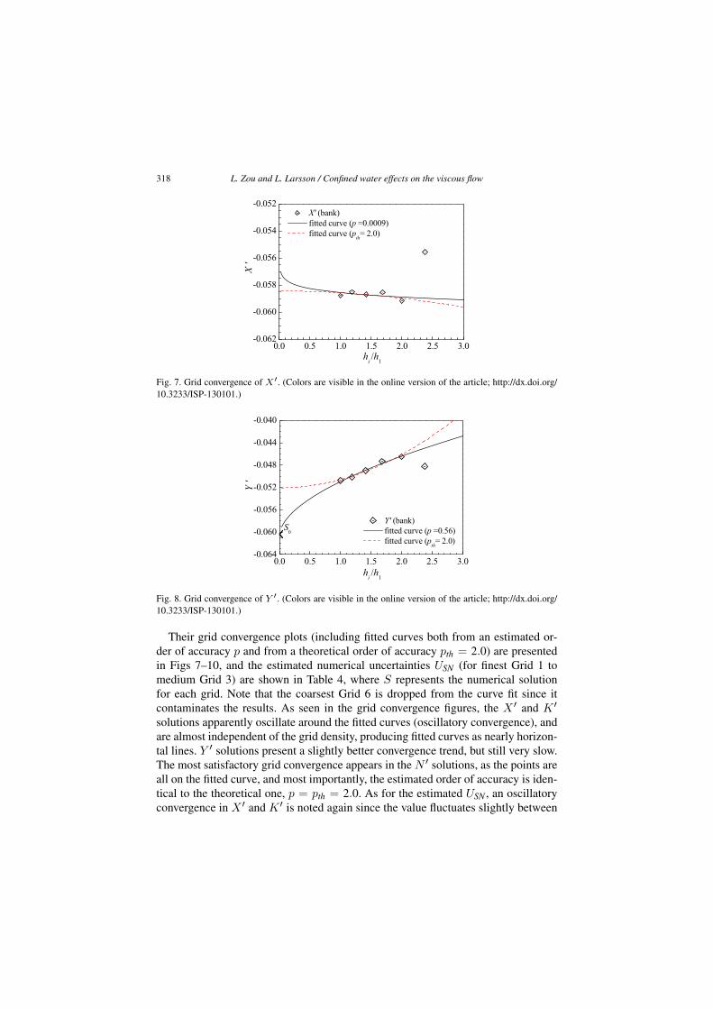
Fig. 7. Grid convergence of X′. (Colors are visible in the online version of the article; http://dx.doi.org/10.3233/ISP-130101.)

Fig. 8. Grid convergence of Y ′. (Colors are visible in the online version of the article; http://dx.doi.org/10.3233/ISP-130101.)

Their grid convergence plots (including fitted curves both from an estimated or-der of accuracy p and from a theoretical order of accuracy pth = 2.0) are presentedin Figs 7–10, and the estimated numerical uncertainties USN (for finest Grid 1 tomedium Grid 3) are shown in Table 4, where S represents the numerical solutionfor each grid. Note that the coarsest Grid 6 is dropped from the curve fit since itcontaminates the results. As seen in the grid convergence figures, the X ′ and K ′

solutions apparently oscillate around the fitted curves (oscillatory convergence), andare almost independent of the grid density, producing fitted curves as nearly horizon-tal lines. Y ′ solutions present a slightly better convergence trend, but still very slow.The most satisfactory grid convergence appears in the N ′ solutions, as the points areall on the fitted curve, and most importantly, the estimated order of accuracy is iden-tical to the theoretical one, p = pth = 2.0. As for the estimated USN , an oscillatoryconvergence in X ′ and K ′ is noted again since the value fluctuates slightly between


Fig. 9. Grid convergence of K′. (Colors are visible in the online version of the article; http://dx.doi.org/10.3233/ISP-130101.)

Fig. 10. Grid convergence of N ′. (Colors are visible in the online version of the article; http://dx.doi.org/10.3233/ISP-130101.)

Table 4

Numerical uncertainties of X′, Y ′ and K′, N ′

X′ Y ′ K′ N ′

p 0.0009 0.56 0.004 2.00

|USN%S|1 3.32 24.45 4.95 4.54

|USN%S|2 3.34 26.21 4.91 6.67

|USN%S|3 3.33 29.91 4.90 8.54

Grid 1, Grid 2 and Grid 3. Uncertainties in Y ′ and N ′ tend to be converged. However,Y ′ presents a slower convergence and its numerical uncertainty is much larger.

From the grid convergence study, it seems very difficult to obtain grid convergencein bank-effects computations, even with a fine grid discretization (i.e. approximately,


8 million grid points). Considering both the accuracy and the computing expense,a density similar to that of Grid 3 was adopted in the systematic computations.

At the first stage of systematic investigations, the computations were made for thetests with only non-rotating propeller in Canal A. The EASM model was applied andto simplify the computation, the still propeller was not included. The measured totalresistance with deducted thrust was used for direct comparison with the predictedresistance (namely X ′). Following a procedure in the ASME V&V 20 2009 stan-dard [1], a formal validation study was performed for the test condition h/T = 1.1and yB = 1.316 in Canal A, in combination with the experimental data from FHR.

In the procedure, the concepts of a validation uncertainty Uval(U2val ≈ U2

num+U2D)

and a comparison error |E| = |S − D| are introduced. S is the numerical solutionand Unum is its uncertainty. D and UD represent the experimental data and the cor-responding uncertainty. Comparing Uval and |E|, if |E| � Uval, the modeling erroris within the “noise level” imposed by the numerical and experimental uncertainty,and not much can be concluded about the source of the error; but if |E| � Uval, thesign and magnitude of E could be used as to improve the modeling. In the validationstudy, the numerical uncertainty Unum was approximated as the grid discretizationuncertainty USN estimated from the grid convergence study (the iterative uncertaintywas neglected), while the data uncertainty UD was available from FHR [4]. The esti-mated uncertainties and comparison errors for hydrodynamics quantities X ′, Y ′, K ′,N ′ are presented in Table 5, where the measured data (D) are used for normalization.As can be seen from the validation study, Y ′ and N ′ present a larger comparison er-ror than validation uncertainty, implying that there were significant modeling errorsin computations and/or measurements.

An investigation of modeling errors in the computations was then carried out byevaluating the influence of neglected waves, non-free sinkage and trim, turbulencemodeling and absence of propeller. The investigation indicated that the wave effectwas negligible, and the influence of sinkage and trim was generally very small, how-ever, it could not be neglected for the K ′ and N ′ moments at the very shallow waterdepth (h/T = 1.1). As for the turbulence model, the Menter k–ω SST model wasapplied for the same computations and it produced slightly better results than theEASM model. Furthermore, including the non-rotating propeller was shown to beimportant, especially for the longitudinal force X ′.

According to the investigation of modeling errors, the computations should beimproved to increase the accuracy taking the sources of modeling error into con-sideration. Therefore based on their significance in specific conditions: the Menter

Table 5

Validation results of X′, Y ′, K′, N ′

X′ Y ′ K′ N ′

|UD%D| 4.40 18.80 7.10 2.78

|USN%D| 3.27 8.38 3.57 6.92

|Uval%D| 5.48 20.58 7.95 7.46

|E%D| 1.85 71.99 27.19 18.94


k–ω SST model was used for turbulence modeling, the computed initial sinkageand trim were added for the tests at the shallowest water depth (h/T = 1.1), whilethe propeller geometry was included in the test conditions with rpm = 0. Finally, thecomputations were extended to all the test conditions for Canal A and Canal B (in Ta-ble 3), including the rotating propeller with varying ship-bank distance. It should benoted that some of the modeling improvements have been presented before [33,34],but the present paper is the first where all improvements have been introduced in asystematic way. Also, the rotating propeller is introduced here for the first time.

8. Propeller simulation

For predicting propeller performance, the non-rotating propeller (zero rpm) wassimply treated as a fixed appendage composed of propeller shaft and four blades. InSHIPFLOW, the rotating propeller is approximated by body forces in the propellerdisc, specified as a cylindrical component grid embedded into the hull grid. Theforces, transferred to XCHAP, are obtained from a lifting line potential flow modelwith an infinite number of blades. Therefore, the force at each point in the propellerdisc is independent of time, approximating a propeller-induced steady flow. The lift-ing line model is interactively coupled with the XCHAP at every ten iteration steps,and the effective wake field and the forces are consequently produced. Thus, thefluid flow passing through the volume grid cells at the propeller disc is acceleratedand the propeller behavior is simulated. More comprehensive specifications of thislifting line model are given in [18,32], and some early applications of this model areavailable in [11,32].

The main computational settings have been introduced in previous sections. How-ever, the propeller grids were not discussed. Examples of the hull-propeller-ruddersurface meshes are presented in Fig. 11(a) and (b) with coarse densities for clarity.Note the difference in grids for the non-rotating and rotating propellers.

Fig. 11. Surface meshes of hull, propeller and rudder. (a) With non-rotating propeller. (b) With rotatingpropeller (body force).


9. Forces and moments

In this section, hydrodynamic forces X ′, Y ′ and moments K ′, N ′ from varyingwater depths and ship-bank distances in Canal A and Canal B are presented. Thepredicted flow field will be shown in the following sections. All the computed forcesand moments are compared with the test data from FHR. It should be noticed thatthe measured data were obtained in a confidential project, so that the absolute valuesof the data and computed results are hidden in the following figures, and only zerovalues are given for reference. Results from the variation of water depth are shown inFigs 12 and 13 for Canal A and B respectively. As for the varying ship-bank distanceat h/T = 1.35, results with the non-rotating (0-rpm) and rotating propeller (self) arepresented in Fig. 14 for Canal A and in Fig. 15 for Canal B.

Fig. 12. X′, Y ′ force and K′, N ′ moment versus h/T in Canal A. (a) X′, Y ′ force. (b) K′, N ′ moment.(Colors are visible in the online version of the article; http://dx.doi.org/10.3233/ISP-130101.)

Fig. 13. X′, Y ′ force and K′, N ′ moment versus h/T in Canal B. (a) X′, Y ′ force. (b) K′, N ′ moment.(Colors are visible in the online version of the article; http://dx.doi.org/10.3233/ISP-130101.)


Fig. 14. X′, Y ′ force and K′, N ′ moment versus yB in Canal A. (a) X′, Y ′ force. (b) K′, N ′ moment.(Colors are visible in the online version of the article; http://dx.doi.org/10.3233/ISP-130101.)

Fig. 15. X′, Y ′ force and K′, N ′ moment versus yB in Canal B. (a) X′, Y ′ force. (b) K′, N ′ moment.(Colors are visible in the online version of the article; http://dx.doi.org/10.3233/ISP-130101.)

Compared with measurements, the tendencies of hydrodynamic forces and mo-ments are captured well in both canals. As seen in Figs 12 and 13, the X ′ force andK ′ moment increase when the hull bottom approaches the seabed, while the Y ′ force(a suction force towards the bank) behaves in a different way. It is almost unchangedbetween h/T = 1.5 and 1.35, but drops rapidly between h/T = 1.35 and 1.1. TheN ′ moment shows a monotonic increase for diminishing water depth, but is verysmall for the larger depths. The tendencies are very similar for both canals.

Results for varying bank distance at the same water depth h/T = 1.35 are pre-sented in Figs 14 and 15. The cases with non-rotating propeller exhibit good corre-spondence between computed X ′ results and measured data and the trends are wellpredicted for the Y ′ force and K ′ and N ′ moments. It is seen that both forces, X ′

and Y ′, increase monotonically when the bank is approached, as does the heeling


moment K ′. The N ′ moment is almost constant and very small over the whole rangeof distances. Again, the trends are very similar in both canals.

For the rotating propeller, the only available data is for the closest distance. Thereis generally a good prediction of the change of the variables at this distance due tothe propeller. This holds for X ′, Y ′ and N ′ and for both canals. However, the changein K ′ has the wrong sign. All predicted forces and moments exhibit an increase dueto the propeller. In particular, the N ′ moment changes from very small to significant.

10. Pressure distributions

To facilitate the understanding of predicted viscous forces and moments and ofthe mechanism of confined-water effects, this section presents the predicted pressuredistributions on the hull (CP , normalizing the pressure by 0.5ρU2), which have adirect connection with the resulting forces and moments. In particular, the pressuredifference between the two sides of the hull is shown below each pressure distribu-tion. The purpose is to ensure a straightforward impression of its contribution to theforces and moments, among which contributions to the lateral force Y ′ and yaw mo-ment N ′ are of most interest. Considering the fact that the starboard side of the hullalways faces the close side bank and encounters the largest influence from this bank,the pressure difference ΔCP (S−P ) is presented on the starboard side and its value isobtained by subtracting the pressure on the port side from that on the starboard side(S − P ). It should be mentioned that no measured flow field is available, thereforein this and following sections, only computed flow field will be presented.

In Fig. 16(a)–(c), CP and ΔCP (S−P ) for varying water depth with non-rotatingpropeller in Canal A are presented, while results in Canal B are shown inFig. 17(a)–(c). Solid contour lines represent positive pressure, while dashed contourlines indicate negative values. A clear difference in the pressure distribution betweenthe water depths at this specific ship-bank distance is shown in these figures. Thelarger the clearance between the hull and the seabed, the smaller the pressure varia-tions along the hull.

In general, a high pressure region is noted at the bow due to stagnation, and itssize and value are largest at the shallowest water depth h/T = 1.1. At this depththere is also a large region of low pressure that covers the parallel middle body ofthe hull in both canals, resulting from the blockage effect. Since in these cases theship-bank distance is also small (yB = 1.316 in Canal A, yB = 0.909 in Canal B),the blockage comes from both the bank and the shallow water. But the shallow-watereffect is slightly stronger, as the largest reduction happens on the bottom of the fore-body, and in Canal B this reduction region is larger because the space between thehull and seabed/bank is smaller due to the sloping bank, see Figs 16(a) and 17(a).

On the fore-body the flow entering into the narrow gap between the hull and theseabed/bank is accelerated, giving rise to the decrease of the pressure. However thelow pressure is not maintained over the whole hull. Instead, the pressure increases(but still with negative values) on the aft-body. The explanation is that the high-speed


Fig. 16. Pressure distribution and difference against h/T (yB = 1.316) in Canal A with non-rotatingpropeller. (a) CP , ΔCP (S−P ) and streamlines on the seabed at h/T = 1.1. (b) CP and ΔCP (S−P )at h/T = 1.35. (c) CP and ΔCP (S−P ) at h/T = 1.5. (Colors are visible in the online version of thearticle; http://dx.doi.org/10.3233/ISP-130101.)

flow from the bow is slowed down. Some of the flow escapes towards the port side.This is clearly seen from the streamlines over the seabed in Canal A, seen from thebottom of the seabed in Fig. 16(a). A remarkable cross flow towards the port side isdeveloped under the fore-body, so the flow speed at the stern is reduced comparingwith that at the fore-body. The notable flow separation at the stern at the shallowestwater depth also gives rise to a large pressure difference between the bow and stern,thus a large resistance (X ′ force) is expected. This will be discussed in a separatesection below.


Fig. 17. Pressure distribution and difference against h/T (yB = 0.909) in Canal B with non-rotat-ing propeller. (a) CP and ΔCP (S−P ) at h/T = 1.1. (b) CP and ΔCP (S−P ) at h/T = 1.35.(c) CP and ΔCP (S−P ) at h/T = 1.5. (Colors are visible in the online version of the article;http://dx.doi.org/10.3233/ISP-130101.)

Turning next to the pressure difference between starboard and port sides for un-derstanding the trends of the forces and moments in Figs 12 and 13, a decrease ofthe pressure difference is noted with an increasing clearance between the hull and theseabed. At all water depths, however, a positive difference is presented at the bowand stern, while negative difference is shown on the parallel middle body. The for-mer generates a force pushing the hull away from the side bank, and the latter is anattraction force towards the bank. At h/T = 1.1, the region with negative pressuredifference covers the whole parallel middle body and generates a large force towardsthe bank. However the positive pressure differences at the bow has a large magnitudeand produces a large repulsion force which more or less balances with the attraction.Therefore, the Y ′ force is relatively small at the smallest water depth. With an in-crease of water depth, the positive pressure at the bow is dramatically reduced andthe pressure at the stern contributes very little, so the negative pressure dominatesand a larger attraction force (Y ′) is produced. While the whole hull is attracted to-


wards the bank, a bow-out yaw moment N ′ is produced as the positive pressure atthe bow is much larger than that at the stern. N ′ is reduced with increasing waterdepth due to the decrease of the pressure difference at the bow. Thus, using the pres-sure distributions, the tendencies of forces and moments against water depth can beexplained.

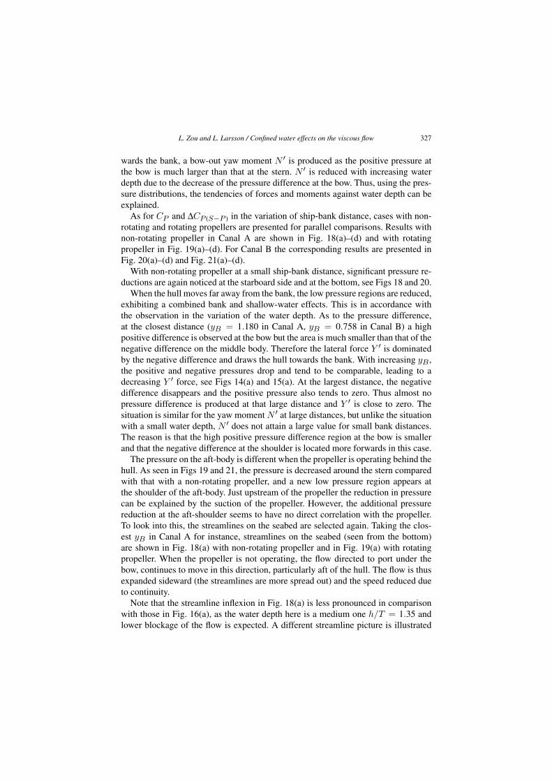
As for CP and ΔCP (S−P ) in the variation of ship-bank distance, cases with non-rotating and rotating propellers are presented for parallel comparisons. Results withnon-rotating propeller in Canal A are shown in Fig. 18(a)–(d) and with rotatingpropeller in Fig. 19(a)–(d). For Canal B the corresponding results are presented inFig. 20(a)–(d) and Fig. 21(a)–(d).

With non-rotating propeller at a small ship-bank distance, significant pressure re-ductions are again noticed at the starboard side and at the bottom, see Figs 18 and 20.

When the hull moves far away from the bank, the low pressure regions are reduced,exhibiting a combined bank and shallow-water effects. This is in accordance withthe observation in the variation of the water depth. As to the pressure difference,at the closest distance (yB = 1.180 in Canal A, yB = 0.758 in Canal B) a highpositive difference is observed at the bow but the area is much smaller than that of thenegative difference on the middle body. Therefore the lateral force Y ′ is dominatedby the negative difference and draws the hull towards the bank. With increasing yB ,the positive and negative pressures drop and tend to be comparable, leading to adecreasing Y ′ force, see Figs 14(a) and 15(a). At the largest distance, the negativedifference disappears and the positive pressure also tends to zero. Thus almost nopressure difference is produced at that large distance and Y ′ is close to zero. Thesituation is similar for the yaw moment N ′ at large distances, but unlike the situationwith a small water depth, N ′ does not attain a large value for small bank distances.The reason is that the high positive pressure difference region at the bow is smallerand that the negative difference at the shoulder is located more forwards in this case.

The pressure on the aft-body is different when the propeller is operating behind thehull. As seen in Figs 19 and 21, the pressure is decreased around the stern comparedwith that with a non-rotating propeller, and a new low pressure region appears atthe shoulder of the aft-body. Just upstream of the propeller the reduction in pressurecan be explained by the suction of the propeller. However, the additional pressurereduction at the aft-shoulder seems to have no direct correlation with the propeller.To look into this, the streamlines on the seabed are selected again. Taking the clos-est yB in Canal A for instance, streamlines on the seabed (seen from the bottom)are shown in Fig. 18(a) with non-rotating propeller and in Fig. 19(a) with rotatingpropeller. When the propeller is not operating, the flow directed to port under thebow, continues to move in this direction, particularly aft of the hull. The flow is thusexpanded sideward (the streamlines are more spread out) and the speed reduced dueto continuity.

Note that the streamline inflexion in Fig. 18(a) is less pronounced in comparisonwith those in Fig. 16(a), as the water depth here is a medium one h/T = 1.35 andlower blockage of the flow is expected. A different streamline picture is illustrated


Fig. 18. Pressure distribution and difference against yB (h/T = 1.35) in Canal A with non-rotatingpropeller. (a) CP , ΔCP (S−P ) and streamlines at yB = 1.180. (b) CP and ΔCP (S−P ) at yB = 1.316.(c) CP and ΔCP (S−P ) at yB = 1.961. (d) CP and ΔCP (S−P ) at yB = 2.431. (Colors are visible inthe online version of the article; http://dx.doi.org/10.3233/ISP-130101.)

in Fig. 19(a) with a rotating propeller. Passing over the bow, a similar cross flowis generated towards the port side. However after the mid-ship, the flow turns backtowards the starboard side due to suction of the operating propeller. Near the sternthe flow moves to starboard, rather than to port. There is thus a concentration of the


Fig. 19. Pressure distribution and difference against yB (h/T = 1.35) in Canal A with rotating propeller.(a) CP , ΔCP (S−P ) and streamlines at yB = 1.180. (b) CP and ΔCP (S−P ) at yB = 1.316. (c) CPand ΔCP (S−P ) at yB = 1.961. (d) CP and ΔCP (S−P ) at yB = 2.431. (Colors are visible in theonline version of the article; http://dx.doi.org/10.3233/ISP-130101.)

streamlines to starboard and the speed is high, giving rise to the pressure reductionin that region. Comparing the cases with non-rotating and rotating propeller, moresuction force (Y ′) is generated on the hull with rotating propeller as greater lowpressure area is produced on the parallel middle body, starboard side. As to the N ′

moment the pressure differences at the bow are almost unchanged, while with the


Fig. 20. Pressure distribution and difference against yB (h/T = 1.35) in Canal B with non-rotatingpropeller. (a) CP and ΔCP (S−P ) at yB = 0.758. (b) CP and ΔCP (S−P ) at yB = 0.909. (c) CP andΔCP (S−P ) at yB = 1.632. (d) CP and ΔCP (S−P ) at yB = 2.173. (Colors are visible in the onlineversion of the article; http://dx.doi.org/10.3233/ISP-130101.)

rotating propeller the pressure is reduced at the stern, starboard side, contributing toa higher bow-out N ′ moment.

11. Streamlines on hull surface and horizontal planes

As shown above, the predicted pressure distribution offers a global view of theflow around the hull and an explanation of the forces and moments (particularly Y ′


Fig. 21. Pressure distribution and difference against yB (h/T = 1.35) in Canal B with rotating pro-peller. (a) CP and ΔCP (S−P ) at yB = 0.758. (b) CP and ΔCP (S−P ) at yB = 0.909. (c) CP andΔCP (S−P ) at yB = 1.632. (d) CP and ΔCP (S−P ) at yB = 2.173. (Colors are visible in the onlineversion of the article; http://dx.doi.org/10.3233/ISP-130101.)

and N ′) a ship encounters in a canal caused by the shallow-water and bank effects.In the present section, more details of the flow will be presented. The focus is on theaft-body where a massive flow separation occurs. Since this has a large influence onthe X ′ force this will be discussed as well. To highlight the complexity of the flow incanals, a double model KVLCC2 hull in deep water (without any appendage) at thesame Re number is considered for reference. As a benchmark case, it has been testedby many experimental institutes. For instance, the measured limiting streamlines ina wind tunnel were reported by Lee et al. [17].

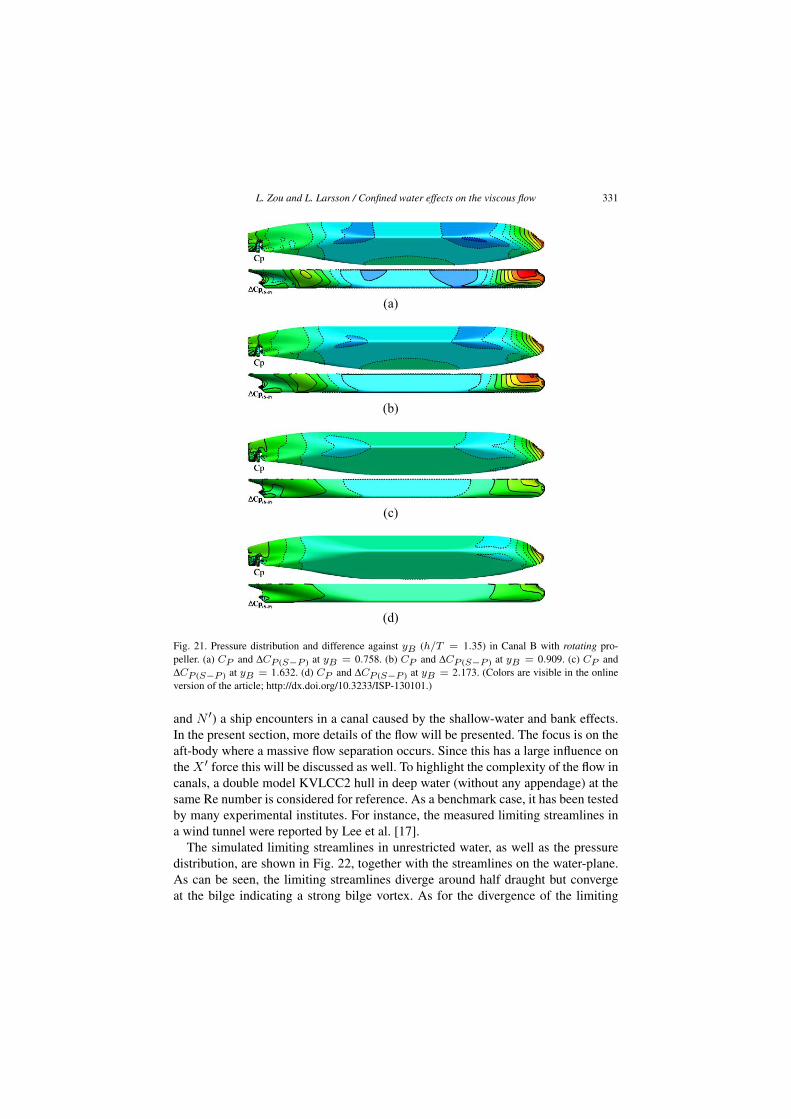
The simulated limiting streamlines in unrestricted water, as well as the pressuredistribution, are shown in Fig. 22, together with the streamlines on the water-plane.As can be seen, the limiting streamlines diverge around half draught but convergeat the bilge indicating a strong bilge vortex. As for the divergence of the limiting


streamlines near the stern, at a saddle point S1 the flow partly goes upwards towardsthe water-plane and partly almost vertically downwards to the propeller shaft whereanother saddle point S2 is formed. A small bubble separation is found at the keel.The predicted limiting streamlines agree very well with the measurements by Leeet al. [17]. Negative pressures are noted at the aft-shoulder and bilge due to thelarge curvature of the hull surface; while towards the stern positive pressures areindicated.

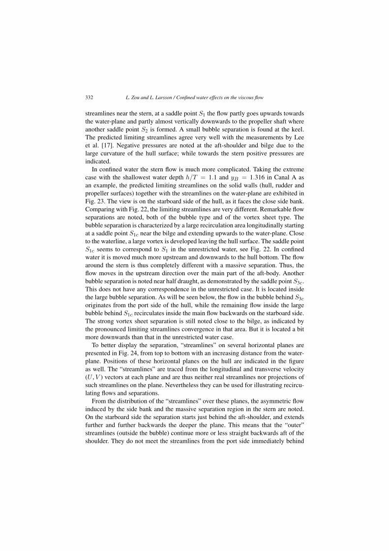
In confined water the stern flow is much more complicated. Taking the extremecase with the shallowest water depth h/T = 1.1 and yB = 1.316 in Canal A asan example, the predicted limiting streamlines on the solid walls (hull, rudder andpropeller surfaces) together with the streamlines on the water-plane are exhibited inFig. 23. The view is on the starboard side of the hull, as it faces the close side bank.Comparing with Fig. 22, the limiting streamlines are very different. Remarkable flowseparations are noted, both of the bubble type and of the vortex sheet type. Thebubble separation is characterized by a large recirculation area longitudinally startingat a saddle point S1c near the bilge and extending upwards to the water-plane. Closeto the waterline, a large vortex is developed leaving the hull surface. The saddle pointS1c seems to correspond to S1 in the unrestricted water, see Fig. 22. In confinedwater it is moved much more upstream and downwards to the hull bottom. The flowaround the stern is thus completely different with a massive separation. Thus, theflow moves in the upstream direction over the main part of the aft-body. Anotherbubble separation is noted near half draught, as demonstrated by the saddle point S3c.This does not have any correspondence in the unrestricted case. It is located insidethe large bubble separation. As will be seen below, the flow in the bubble behind S3coriginates from the port side of the hull, while the remaining flow inside the largebubble behind S1c recirculates inside the main flow backwards on the starboard side.The strong vortex sheet separation is still noted close to the bilge, as indicated bythe pronounced limiting streamlines convergence in that area. But it is located a bitmore downwards than that in the unrestricted water case.

To better display the separation, “streamlines” on several horizontal planes arepresented in Fig. 24, from top to bottom with an increasing distance from the water-plane. Positions of these horizontal planes on the hull are indicated in the figureas well. The “streamlines” are traced from the longitudinal and transverse velocity(U ,V ) vectors at each plane and are thus neither real streamlines nor projections ofsuch streamlines on the plane. Nevertheless they can be used for illustrating recircu-lating flows and separations.

From the distribution of the “streamlines” over these planes, the asymmetric flowinduced by the side bank and the massive separation region in the stern are noted.On the starboard side the separation starts just behind the aft-shoulder, and extendsfurther and further backwards the deeper the plane. This means that the “outer”streamlines (outside the bubble) continue more or less straight backwards aft of theshoulder. They do not meet the streamlines from the port side immediately behind


Fig. 22. Streamlines and pressure distributions on a double model KVLCC2 in unrestricted water. (Colorsare visible in the online version of the article; http://dx.doi.org/10.3233/ISP-130101.)

Fig. 23. Streamlines and pressure distributions at h/T = 1.1 and yB = 1.316 in Canal A. (Colors arevisible in the online version of the article; http://dx.doi.org/10.3233/ISP-130101.)

the stern, as they do in an unseparated flow. This means that the high pressure re-gion normally found close to the stern and caused by the concave curvature of thestreamlines in this region is absent. Comparing Figs 23 and 22 this effect is clearlyseen.

Looking at the “streamlines” on the port side, they in fact exhibit a similar be-havior. There is not much concave curvature near the stern. The curvature appearsfurther aft, where the streamlines from the main flow on the two sides meet. There-fore the pressure is not very high even on the port side. (As will be seen below it ishowever slightly larger than on the starboard side.)


Fig. 24. Top view of “streamlines” on horizontal planes. (a) Positions of the horizontal planes. (b) Fromtop to bottom: z/LPP = 0, 0.01, 0.02, 0.03, 0.04, 0.05 and 0.06. (Colors are visible in the online versionof the article; http://dx.doi.org/10.3233/ISP-130101.)


The missing high pressure region on the two sides of the stern causes a consid-erable increase in resistance. This is clearly seen in the plots of the X ′ force inFigs 12(a) and 13(a). For the present shallow water depth the resistance (solid line)is about three times that in unrestricted water (dash-dot line). The effect is reduced atthe largest tested water depth where the ratio is about two. As seen in Fig. 25 the sep-aration zone is reduced with the water depth, but it is still significant at h/T = 1.5.

Turning next to the influence on streamlines by different propeller performance,results of the closest ship-bank distance at h/T = 1.35 in Canal A with non-rotatingand rotating propeller are presented in Figs 26 and 27, respectively. As shown in thelimiting streamline figures, an operating propeller considerably changes the flow infront of it. In general, the propeller suction attracts the flow towards the propellerdisc. There is however, a region of backward flow close to the surface even just infront of the propeller. The details will be explained in the next section.

Fig. 25. Streamlines against water depth in Canal A. (a) h/T = 1.35. (b) h/T = 1.5. (Colors are visiblein the online version of the article; http://dx.doi.org/10.3233/ISP-130101.)


Fig. 26. Streamlines with non-rotating propeller: h/T = 1.35 and yB = 1.180 in Canal A. (Colors arevisible in the online version of the article; http://dx.doi.org/10.3233/ISP-130101.)

Fig. 27. Streamlines with rotating propeller: h/T = 1.35 and yB = 1.180 in Canal A. (Colors are visiblein the online version of the article; http://dx.doi.org/10.3233/ISP-130101.)

12. Hull-propeller-rudder interaction: Local pressure distributions,axial velocity contours and cross-flow vectors

In the present section more details of the flow without and with the rotating pro-peller will be presented for the cases seen in Figs 26 and 27. (The most extremecase with the rotating propeller.) Results are demonstrated by the local pressure dis-tributions (CP ) on the port and starboard sides of the aft-body, together with theaxial velocity contours (U0-rpm or Uself , seen from the stern) on the propeller planex/LPP = −0.4825 and the local cross-flow vectors around the propeller disc. Resultswith non-rotating and rotating propeller are shown in Figs 28 and 29, respectively.

With a non-rotating propeller, the pressure on the whole aft-body is small as ex-plained above. Considering the large differences between the flows on the port andstarboard side, revealed in Fig. 24, the pressures are surprisingly similar on the twosides. Far aft, the pressure is however slightly higher on the port side, which gives


Fig. 28. Local pressure distributions on the surfaces and axial velocity contours/cross-flow vectors at thepropeller plane: h/T = 1.35 and yB = 1.180 in Canal A (non-rotating propeller). (Colors are visible inthe online version of the article; http://dx.doi.org/10.3233/ISP-130101.)


Fig. 29. Local pressure distributions on the surfaces and axial velocity contours/cross-flow vectors at thepropeller plane: h/T = 1.35 and yB = 1.180 in Canal A (rotating propeller). (Colors are visible in theonline version of the article; http://dx.doi.org/10.3233/ISP-130101.)


rise to the negative pressure difference seen in this region in Fig. 18(a). In the upperpart, near the leading edge of the rudder, a high pressure region appears on the portside and a low pressure region is on the opposite side. As mentioned above, thereis a cross-flow from the port side into the separation bubble aft of S3c. This is whatcauses the asymmetric pressure. The cross-flow is also clearly seen in the vector plotin Fig. 28, above the propeller disk. In fact there is a cross-flow in the other directionbelow the propeller disk, but its magnitude is much smaller and it has only a verysmall effect on the symmetry of the pressure.

To indicate the complex flow around the rudder the limiting streamlines there aredisplayed in the figure. On the port side the flow is essentially backwards, as canalso be inferred from the “streamline” plots of Fig. 24. However, on the starboardside the rudder is within the recirculating region of the main separation bubble andthe flow is essentially forwards. Obviously the rudder will not work well under suchconditions.

When the propeller is rotating behind the hull, see Fig. 29, the pressure on theaft-body is decreased, as expected. The high pressure region above and behind thepropeller is also as normally expected. Since the rudder operates in the slipstream,both the pressure and the streamlines have changed completely as compared to thecase of Fig. 28. The stagnation in the upper part of the rudder in Fig. 28 has disap-peared. Inside the propeller slipstream, the port side of the rudder has a high pressurearea around the leading edge above the propeller shaft center-plane and a low pres-sure just below the center-plane. The opposite situation happens to the starboard side.This is a result of the right-handed rotation of the propeller slipstream, as illustratedby the axial velocity contours and the cross-flow vectors on the propeller plane.

Comparing the velocity contours of Figs 28 and 29 it is seen that the low speedregion in the main separation bubble is reduced with the operating propeller, in ac-cordance with the observations for the limiting streamlines. In unrestricted water thenominal wake is of course symmetric but the velocities have an upward component.This gives rise to an asymmetric loading, since the blades going down to starboardencounter a larger angle of attack than those going up to port. Therefore the star-board side of the propeller disk is more heavily loaded than the port one. Lookingat the velocity contours in Fig. 29 it is seen that the velocities to port are larger thanon the other side. This is opposite to what is expected for a right turning propeller,but is due to the fact that the velocities in the nominal wake are much smaller tostarboard. The increase in velocity through the disk is larger on the starboard side.Since the velocity is so small in this region the propeller blades will have to operateat a very large angle of attack, like in bollard pull, and generate a large thrust. This isconsistent with the larger reduction in pressure on the starboard side compared withthe port side due to the propeller, and seen in Fig. 29. It is also consistent with theresults of Fig. 14, where the propeller induces a bow-out moment.

Like in unrestricted water the reduced pressure around the stern creates an in-creased resistance force X ′ (thrust deduction). In Fig. 14 this is seen as the differ-ence between the non-rotating and rotating cases. The magnitude of the effect seemsto be as large as in unrestricted water.


13. Conclusions

Applying a steady state RANS method, confined-water effects on a KVLCC2tanker appended with a rudder and a propeller in two canals have been studied inthe present paper. The selected systematic conditions include both extremely shal-low water depths and close ship-bank distances, which have made the computationsrather difficult. In addition, propeller effects (at a zero propeller rate and at self-propulsion) have been taken into consideration. In earlier work, a grid convergencestudy and a formal validation study followed by an investigation of modeling errorswere performed. Experiences from these preliminary studies provided knowledge ofthe numerical error/uncertainty, and most importantly, of the modeling errors in theRANS computations of this kind. In the present study the best available models wereadopted. The predicted tendencies of viscous forces and moments in terms of vary-ing water depth and ship-bank distance have shown to be qualitatively in accordancewith the measurement data. The emphasis of the present paper is the predicted flowfield, which is used to explain the effect of the confined water.

The predicted pressure distributions have offered an insight into the forces andmoments acting on the hull. A high pressure region appears at the bow of the hulldue to the stagnation. Further downstream the pressure is reduced more than in anunrestricted flow due to the blockage from shallow seabed and/or close side bank.The low pressure region starting from the fore-shoulder covers the whole parallelmiddle body on the starboard side, facing the bank, and is extended towards thestern region. However, the pressure gradually increases backwards due to the factthat the flow “escapes” to the port side under the bottom. At the stern the pressure ismuch lower than in an undisturbed flow due to a massive separation on the starboardside, starting near the aft shoulder. This separation causes a large recirculation zoneextending backwards behind the rudder. The whole flow around the stern therebygets asymmetric. In an unrestricted flow the streamlines from the two sides meet atthe stern and create a high pressure. In the present case the streamlines outside theseparation bubble meet further aft, so no high pressure is created at the stern. Thiscauses a large increase in resistance, for the most extreme case about three times, ascompared with the unrestricted water case.

The propeller increases the velocity around the aft-body, just like in unrestrictedflow, but due to the very low velocities on the starboard side, this half of the propellergets more heavily loaded. It therefore sucks more flow on the starboard side and thereduced pressure causes a bow-out moment on the hull with the rotating propeller.

Acknowledgements

The present work was funded by Chalmers University of Technology, Swedenand the China Scholarship Council. Computing resources were provided by C3SE,Chalmers Centre for Computational Science and Engineering. The authors thank


Mr. Guillaume Delefortrie (Flanders Hydraulics Research, Belgium) and Mr. EvertLataire (Maritime Technology Division, Ghent University, Belgium) for providingthe experimental data.

Appendix. Grid convergence study

The grid convergence study followed the method by Eça et al. [7], based on theRichardson Extrapolation (RE) and a Grid Convergence Index (GCI) proposed byRoache [26]. With Richardson Extrapolation, the grid discretization error δRE in anumerical solution can be expressed in a power series in the step size as:

δRE = Si − S0 = αhpi ,

where Si is the solution on the ith grid (i = 1, 2, . . . ,ng , ng – available number ofgrids ng > 3); S0 is the extrapolated solution to the zero step size; α is a constant;hi represents the step size (grid spacing) of the ith grid and p is the order of accuracyin the numerical method.

To determine the three unknowns (S0, α, p) in the equation above with more thanthree solutions, the observed order of accuracy p can be estimated through the curvefit of the Least Squares Root approach, minimizing the following function:

f (S0,α, p) =

√√√√ ng∑i=1

(Si −

(S0 + αh

pi

))2.

The convergence condition is decided as below:

1. Monotonic convergence: p > 0.2. Oscillatory convergence: nch � INT(ng/3), where nch is the number of

triplets with (Si+1 − Si)(Si − Si−1) < 0.3. Anomalous behaviour: otherwise.

Three alternative error estimators are then introduced (the first two estimators areobtained from curve fit as well):

δ02RE = Si − S0 = α02h

2i ,

δ12RE = Si − S0 = α11hi + α12h

2i ,

δΔM=

ΔM

(hng/h1) − 1,

where ΔM is the data range, ΔM = max(|Si − Sj |), 1 � i, j � ng , hng is the stepsize of the ngth grid.


The numerical uncertainty still follows the form in [26]: USN = FS · |δRE|, FS isa factor of safety. Based on the convergence condition, the numerical uncertainty isformulated as follows:

1. Monotonic convergence:

a. 0.95 � p � 2.05: USN = 1.25δRE + USD,b. p � 0.95: USN = min(1.25δRE + USD, 3δ12

RE + U12SD),

c. p � 2.05: USN = max(1.25δRE + USD, 3δ02RE + U02

SD).

2. Oscillatory convergence: USN = 3δΔM .3. Anomalous behaviour: USN = min(3δΔM

, 3δ12RE + U12

SD), where USD, U02SD, U12

SDare standard deviations of the curve fits.

References

[1] ASME V&V 20–2009, Standard for Verification and Validation in Computational Fluid Dynamicsand Heat Transfer, American Society of Mechanical Engineers, New York, 2009.

[2] L. Broberg, B. Regnström and M. Östberg, SHIPFLOW theoretical manual, FLOWTECH Interna-tional AB, Gothenburg, Sweden, 2007.

[3] P.W. Ch’ng, L.J. Doctors and M.R. Renilson, A method of calculating the ship-bank interactionforces and moments in restricted water, International Shipbuilding Progress 40(421) (1993), 7–23.

[4] G. Delefortrie, K. Eloot and F. Mostaert, SIMMAN 2012: Execution of model tests with KCS andKVLCC2. Version 2_0, WL Rapporten, 846_01, Flanders Hydraulics Research, Antwerp, Belgium,2011.

[5] G.B. Deng, P. Queutey and M. Visonneau, Three-dimensional flow computation with Reynoldsstress and algebraic stress models, in: Engineering Turbulence Modeling and Experiments, Vol. 6,W. Rodi and M. Mulas, eds, Elsevier, 2005, pp. 389–398.

[6] E. Dick and J. Linden, A multi-grid method for steady incompressible Navier–Stokes equationsbased on flux difference splitting, International Journal for Numerical Methods in Fluids 14 (1992),1311–1323.

[7] L. Eça, G. Vaz and M. Hoekstra, Code verification, solution verification and validation in RANSsolvers, in: Proceedings of ASME 29th International Conference OMAE2010, June 6–11, 2010,Shanghai, China.

[8] L. Eça, G. Vaz and M. Hoekstra, A verification and validation exercise for the flow over a backwardfacing step, V European Conference on Computational Fluid Dynamics, ECCOMAS CFD 2010,J.C.F. Pereira and A. Sequeira, eds, June 2010, Lisbon.

[9] T.B. Gatski and C.G. Speziale, On explicit algebraic stress models for complex turbulent flows,Journal of Fluid Mech. 254 (1993), 59–78.

[10] T. Gourlay, Slender-body methods for predicting ship squat, Ocean Engineering 35(2) (2008),191–200.

[11] K.J. Han, Numerical optimization of hull/propeller/rudder configurations, Doctor thesis, ChalmersUniversity of Technology, Gothenburg, Sweden, 2008.

[12] A. Hellsten and S. Laine, Extension of the k–ω-SST turbulence model for flows over rough surfaces,in: AIAA-97-3577, 1997, pp. 252–260.

[13] International Conference on Ship Maneuvering in Shallow and Confined Water: Bank Effects,Antwerp, Belgium, 2009, available at: http://www.bankeffects.ugent.be/index.html.

[14] L. Larsson and H. Raven (eds), Ship Resistance and Flow, Society of Naval Architects and MarineEngineers, New York, 2010.


[15] E. Lataire, M. Vantorre and K. Eloot, Systematic model tests on ship-bank interaction effects, in:Proceedings of International Conference on Ship Maneuvering in Shallow and Confined Water:Bank Effects, Antwerp, Belgium, May 2009.

[16] C.K. Lee and S.G. Lee, Investigation of ship maneuvering with hydrodynamic effects between shipand bank, Journal of Mechanical Science and Technology 22(6) (2008), 1230–1236.

[17] S.J. Lee, H.R. Kim, W.J. Kim and S.H. Van, Wind tunnel tests on flow characteristics of the KRISO3600 TEU containership and 300K VLCC double-deck ship models, Journal of Ship Research 47(1)(2003), 24–38.

[18] D.Q. Li, Investigation on the propeller-rudder interaction by numerical methods, Doctor thesis,Chalmers University of Technology, Gothenburg, Sweden, 1994.

[19] D.Q. Li, M. Leer-Andersen, P. Ottosson and P. Trägårdh, Experimental investigation of bank effectsunder extreme conditions, in: Practical Design of Ships and Other Floating Structures, ElsevierScience, Oxford, 2001, pp. 541–546.

[20] D.C. Lo, D.T. Su and J.M. Chen, Application of computational fluid dynamics simulations to theanalysis of bank effects in restricted waters, Journal of Navigation 62 (2009), 477–491.

[21] F.R. Menter, Zonal two equation k–ω turbulence models for aerodynamic flows, in: 24th FluidDynamics Conference, Orlando, AIAA paper 93-2906, 1993.

[22] Q.M. Miao, J.Z. Xia, A.T. Chwang et al., Numerical study of bank effects on a ship travellingin a channel, in: Proceedings of 8th International Conference on Numerical Ship Hydrodynamics,Busan, Korea, 2003.

[23] J.N. Newman, The green function for potential flow in a rectangular channel, Journal of EngineeringMathematics, Anniversary Issue (1992), 51–59.

[24] N. Norrbin, Bank clearance and optimal section shape for ship canals, in: 26th PIANC InternationalNavigation Congress, Brussels, Belgium, Section 1, Subject 1, 1985, pp. 167–178.

[25] N. Norrbin, Bank effects on a ship moving through a short dredged channel, in: 10th ONR Sympo-sium on Naval Hydrodynamics, Cambridge, MA, 1974.

[26] P.J. Roache, Verification and validation in computational science and engineering, Hermosa Pub-lishers, Albuquerque, 1998.

[27] P.L. Roe, Approximate Riemann solvers, parameter vectors, and difference schemes, Journal ofComputational Physics 43 (1981), 357–372.

[28] E.O. Tuck, A systematic asymptotic expansion procedure for slender ships, Journal of Ship Research8 (1964), 15–23.

[29] E.O. Tuck, Shallow water flows past slender bodies, Journal of Fluid Mechanics 26 (1966), 81–95.[30] M. Vantorre, G. Delefortrie et al., Experimental investigation of ship-bank interaction forces,

in: Proceedings of International Conference on Marine Simulation and Ship Maneuverability,MARSIM’03, Kanazawa, Japan, 2003.

[31] H.M. Wang, Z.J. Zou, Y.H. Xie and W.L. Kong, Numerical study of viscous hydrodynamic forceson a ship navigating near bank in shallow water, in: Proceedings of the Twentieth InternationalOffshore and Polar Engineering Conference, June 20–25, 2010, Beijing, China.

[32] D.H. Zhang, Numerical computation of ship stern/propeller flow, Doctor thesis, Chalmers Universityof Technology, Gothenburg, Sweden, 1990.

[33] L. Zou, CFD predictions including verification and validation of hydrodynamic forces and momentson a ship in restricted waters, Licentiate thesis, Chalmers University of Technology, Gothenburg,Sweden, June 2011.

[34] L. Zou, L. Larsson, G. Delefortrie and E. Lataire, CFD prediction and validation of ship-bank inter-action in a canal, in: Proceedings of 2nd International Conference on Ship Maneuvering in Shallowand Confined Water, Trondheim, Norway, 2011.

[35] L. Zou, L. Larsson and M. Orych, Verification and validation of CFD predictions for a maneuveringtanker, Journal of Hydrodynamics, Ser. B 22(5) (2010), 438–445.

Documents

Confined water effects on the viscous flow around a tanker