Embed Size (px)
Citation preview

Confirmatory Factor AnalysisUsing OpenMx & R
(CFA) Practical Session
Timothy C. Bates

Confirmatory Factor Analysisto test theory
• Are there 5 independent domains of personality?
• Do domains have facets?• Is Locus of control the same as primary
control?• Is prosociality one thing , or three?• Is Grit independent of Conscientiousness?

Prosocial Obligations
• Prosociality covers several domains, e.g.– Workplace: voluntary overtime– Civic life: Giving evidence in court– Welfare of others: paying for other’s healthcare
• CFA can test the fit of theories– Which hypothesised model fits best?
• 3 indicators of one factor?• 3 correlated factors?• 3 independent factors?

Factor structure of Prosociality
• Distinct domains?
Work1
Work 2
Work 3
Civic 1
Civic 2
Civic 3
Welfare 1
Welfare 2
Welfare 3
Work Civic Welfare

Factor structure of Prosociality
• One underlying prosociality factor?
Work1
Work 2
Work 3
Civic 1
Civic 2
Civic 3
Welfare 1
Welfare 2
Welfare 3
Prosociality

Factor structure of Prosociality
• Hierarchical structure: Common and distinct factors?
Work1
Work 2
Work 3
Civic 1
Civic 2
Civic 3
Welfare 1
Welfare 2
Welfare 3
Work Civic Welfare
Prosociality
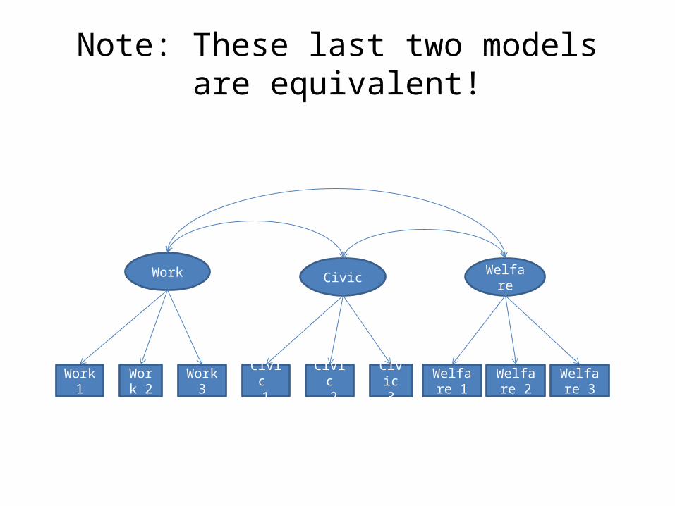
Note: These last two models are equivalent!
Work1
Work 2
Work 3
Civic 1
Civic 2
Civic 3
Welfare 1
Welfare 2
Welfare 3
Work Civic Welfare

CFA with R & OpenMx
• library(OpenMx)• What is OpenMx?
– “OpenMx is free and open source software for use with R that allows estimation of a wide variety of advanced multivariate statistical models.”
• Homepage: http://openmx.psyc.virginia.edu/
• # library(sem)

Our data
• Dataset: Midlife Study of Well-Being in the US (Midus)• Prosocial obligations - c. 1000 individuals
– How much obligation do you feel…• to testify in court about an accident you witnessed?’
[civic]• to do more than most people would do on your kind of
job?’ [work]• to pay more for your healthcare so that everyone had
access to healthcare? [welfare]

Preparatory code
First we need to load OpenMxrequire(OpenMx)
Now lets get the data (R can read data off the web)myData= read.csv("http://www.subjectpool.com/prosocial_data.csv")
? What are the names in the data?summary(myData) # We have some NAs
myData= na.omit(myData) # imputation is another solution
summary(myData)
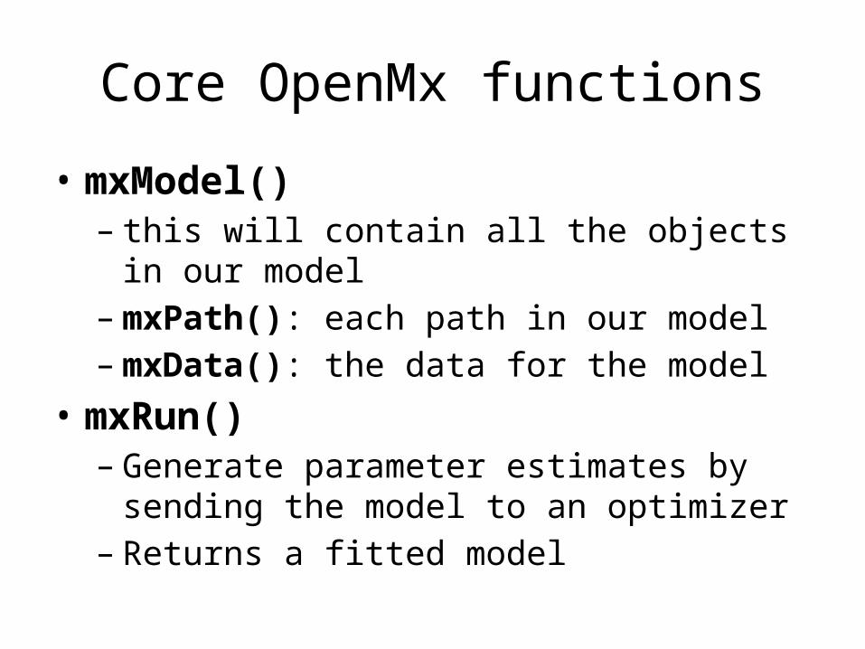
Core OpenMx functions
• mxModel()– this will contain all the objects in our model– mxPath(): each path in our model– mxData(): the data for the model
• mxRun() – Generate parameter estimates by sending the
model to an optimizer– Returns a fitted model
CFA on our competing models
• Three competing models to test today:1. One general factor2. Three uncorrelated factors3. Three correlated factors
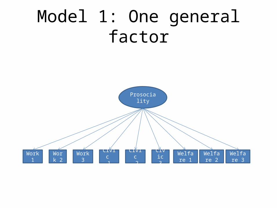
Model 1: One general factor
Work1
Work 2
Work 3
Civic 1
Civic 2
Civic 3
Welfare 1
Welfare 2
Welfare 3
Prosociality
• Quite a bit more code than you have used before:– We’ll go through it step-by-step
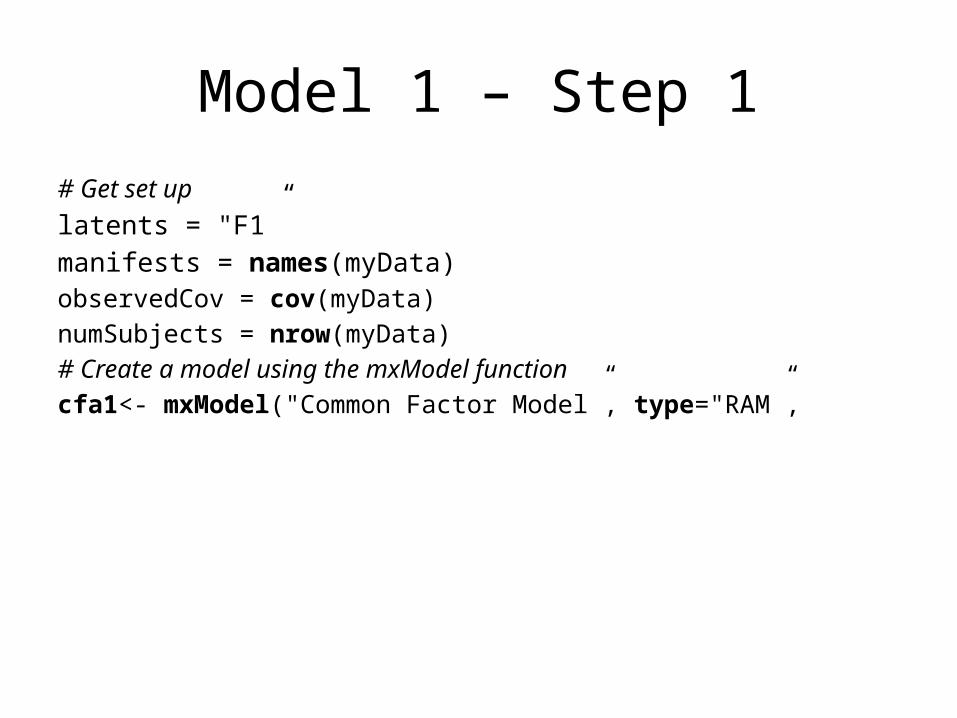
Model 1 – Step 1# Get set uplatents = "F1”manifests = names(myData)observedCov = cov(myData)numSubjects = nrow(myData)# Create a model using the mxModel functioncfa1<- mxModel("Common Factor Model”, type="RAM”,

Model 1 – Step 2# Here we set the measured and latent variables manifestVars = manifests,latentVars = latents,

Model 1 – Step 3# Create residual variance for manifest variables using mxPathmxPath( from=manifests, arrows=2, free=T, values=1, labels=paste("error”, 1:9, sep=“”) ),
# using mxPath, fix the latent factor variance to 1mxPath( from="F1", arrows=2, free=F, values=1, labels ="varF1”),
# Using mxPath, specify the factor loadingsmxPath(from="F1”, to=manifests, arrows=1, free=T, values=1, labels =paste(”l”, 1:9, sep=“”)),
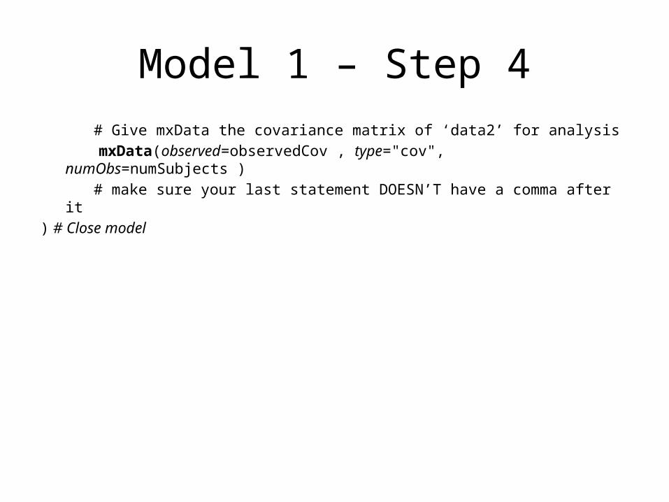
Model 1 – Step 4 # Give mxData the covariance matrix of ‘data2’ for analysis mxData(observed=observedCov , type="cov", numObs=numSubjects ) # make sure your last statement DOESN’T have a comma after it) # Close model
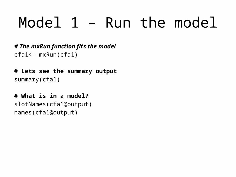
Model 1 – Run the model# The mxRun function fits the modelcfa1<- mxRun(cfa1)
# Lets see the summary outputsummary(cfa1)
# What is in a model?slotNames(cfa1@output)names(cfa1@output)
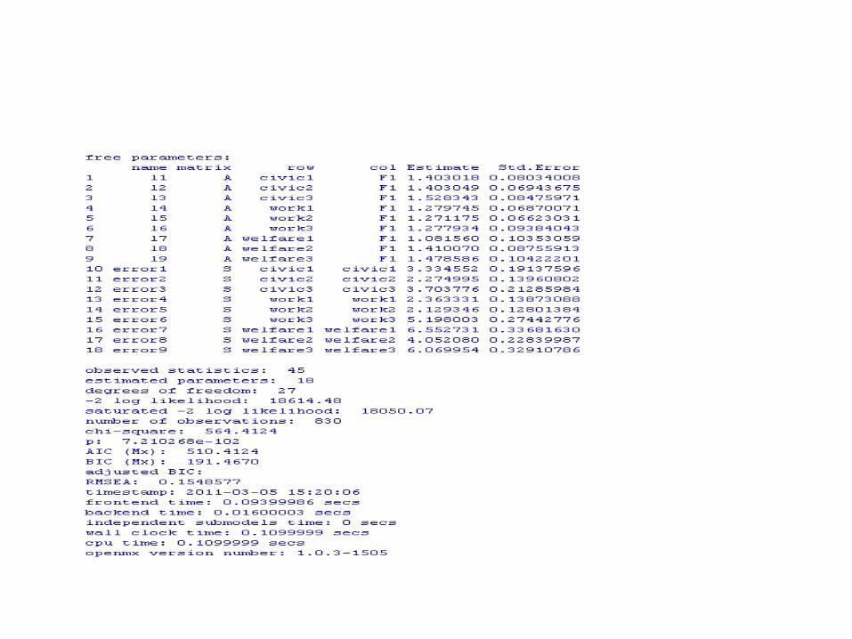

Summary Output
# Ideally, chi-square should be non-significantchi-square: 564.41; p: < .001
# Lower is better for AIC and BICAIC (Mx): 510.41BIC (Mx): 191.47
# < .06 is good fit: This model is a bad fitRMSEA: 0.15
Story so far…
• Model 1 (one common factor) is a poor fit to the data)
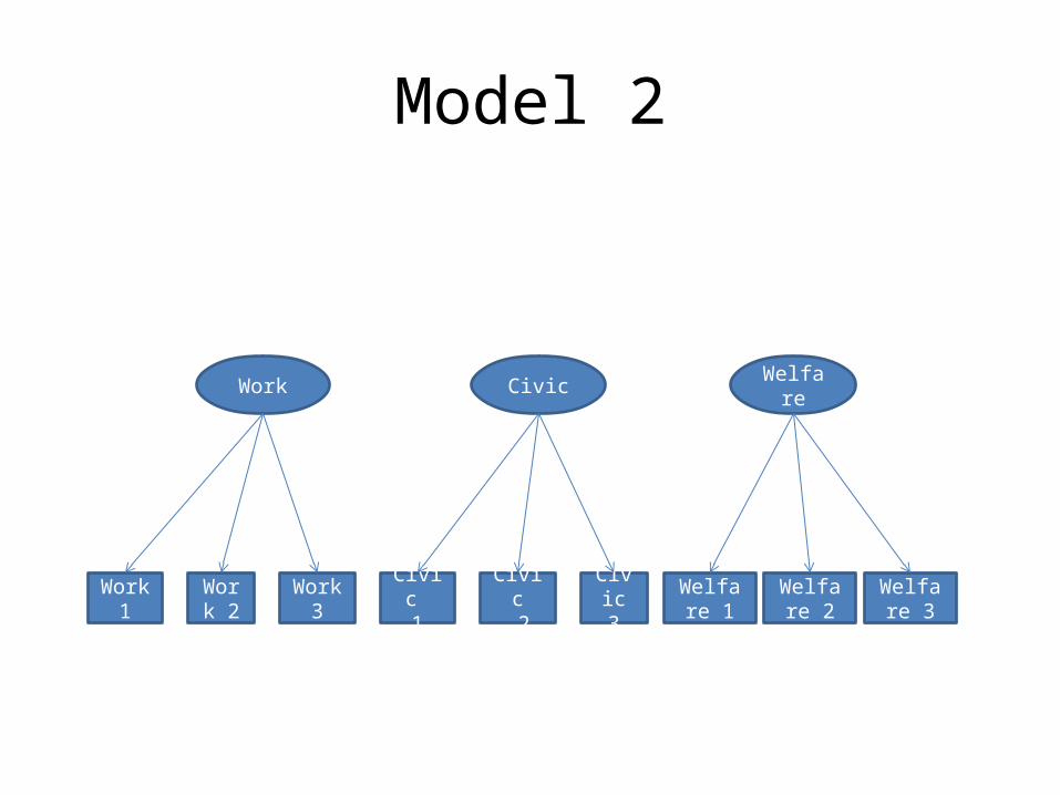
Model 2
Work1
Work 2
Work 3
Civic 1
Civic 2
Civic 3
Welfare 1
Welfare 2
Welfare 3
Work Civic Welfare
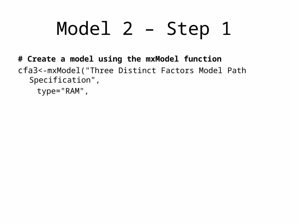
Model 2 – Step 1 # Create a model using the mxModel functioncfa3<-mxModel("Three Distinct Factors Model Path Specification", type="RAM",

Model 2 – Step 2# Here we name the measured variables manifestVars=manifests,
# Here we name the latent variablelatentVars=c("F1","F2", "F3"),

Model 2 – Step 3# Create residual variance for manifest variablesmxPath(from=manifests, arrows=2, free=T,values=1, labels=c("error”, 1:9, sep=“”)),

Model 2 – Step 4# Specify latent factor variances mxPath(from=c("F1","F2", "F3"), arrows=2,free=F, values=1, labels=c("varF1","varF2", "varF3") ),
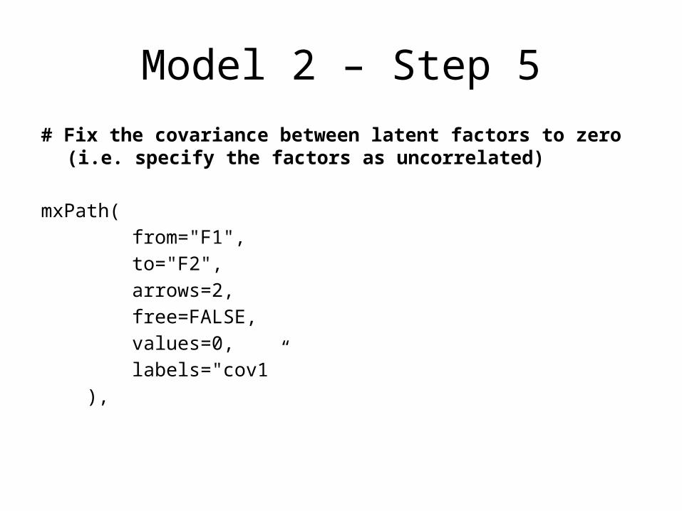
Model 2 – Step 5# Fix the covariance between latent factors to zero (i.e. specify the factors
as uncorrelated)
mxPath( from="F1", to="F2", arrows=2, free=FALSE, values=0, labels="cov1” ),
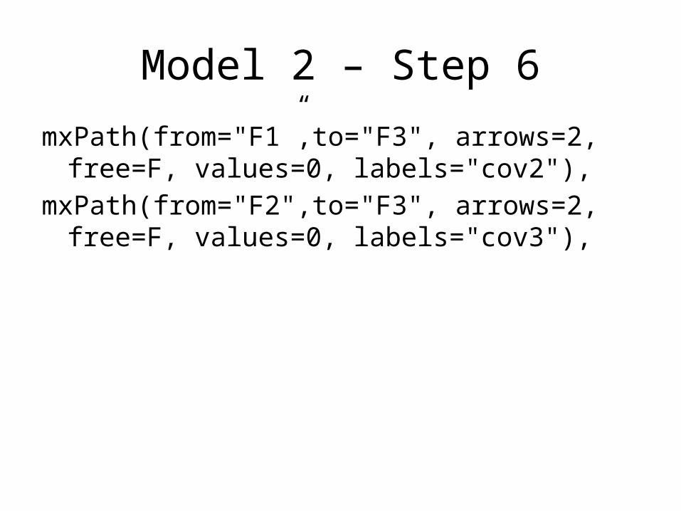
Model 2 – Step 6
mxPath(from="F1”,to="F3", arrows=2, free=F, values=0, labels="cov2"),
mxPath(from="F2",to="F3", arrows=2, free=F, values=0, labels="cov3"),

Model 2 – Step 7
# Specify the factor loading i.e. here we specify that F1 loads on work1, 2, and 3 mxPath( from="F1", to=c("work1","work2","work3"), arrows=1, free=T, values=1, labels=c("l1","l2","l3")),mxPath( from="F2", to=c("civic1","civic2", "civic3"), arrows=1, free=T, values=1, labels=c("l4","l5", "l6")),
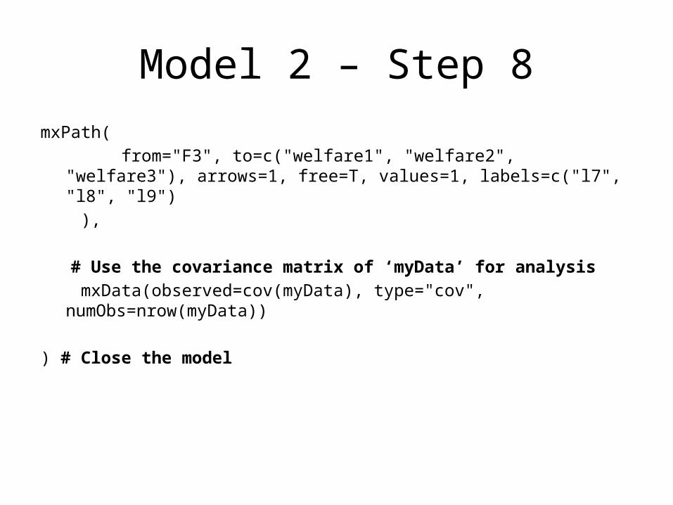
Model 2 – Step 8mxPath( from="F3", to=c("welfare1", "welfare2", "welfare3"), arrows=1, free=T, values=1,
labels=c("l7", "l8", "l9") ),
# Use the covariance matrix of ‘myData’ for analysis mxData(observed=cov(myData), type="cov", numObs=nrow(myData))
) # Close the model
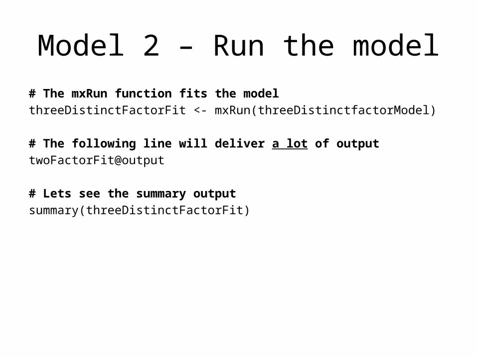
Model 2 – Run the model# The mxRun function fits the modelthreeDistinctFactorFit <- mxRun(threeDistinctfactorModel)
# The following line will deliver a lot of outputtwoFactorFit@output
# Lets see the summary outputsummary(threeDistinctFactorFit)


Summary Output# Ideally, chi-square should be non-significantchi-square: 576.50; p: <.0001
# Lower is better for AIC and BICAIC (Mx): 522.50 BIC (Mx): 197.51
# <.08 is a reasonable fit: This model is a poor fitRMSEA: 0.16
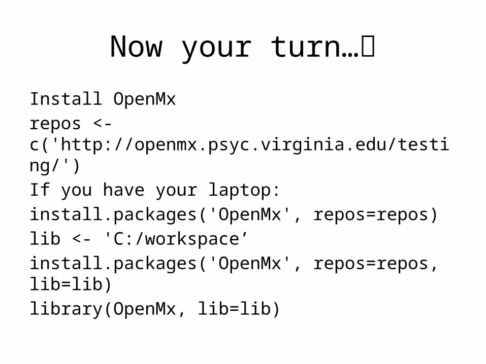
Now your turn…
Install OpenMxrepos <- c('http://openmx.psyc.virginia.edu/testing/')If you have your laptop:install.packages('OpenMx', repos=repos)lib <- 'C:/workspace’install.packages('OpenMx', repos=repos, lib=lib)library(OpenMx, lib=lib)