Confocal fluorescence microscopy of colloidal quantum dots

Confocal fluorescence microscopyof colloidal quantum dots

THESIS

submitted in partial fulfillment of therequirements for the degree of

BACHELOR OF SCIENCEin

PHYSICS

Author : M. van den NieuwenhuijzenStudent ID : 2042096Supervisor : prof. dr. M.P. van ExterSecond corrector : prof. dr. M.A.G.J. Orrit

Leiden, The Netherlands, March 10, 2021

Confocal fluorescence microscopyof colloidal quantum dots

M. van den Nieuwenhuijzen

Huygens-Kamerlingh Onnes Laboratory, Leiden UniversityP.O. Box 9500, 2300 RA Leiden, The Netherlands

March 10, 2021

Abstract

This thesis investigates the fluorescence properties of 605 nm and 655 nmcolloidal quantum dots. Samples with different densities of both types ofquantum dots were created and examined with a confocal fluorescencemicroscope. In particular, the thesis focuses on the spatial distribution ofthe quantum dots on the sample, the characteristics of their luminescencedecay and the effects of blinking and bleaching.Three different methods were used to study the former phenomena. Spa-tial scans of the samples helped to locate the quantum dots and revealedthat they have a high tendency to cluster. Time-resolved measurementsunder pulsed excitation provided information on the luminescence decayand show varying, multi-exponential decay times. Finally, extended (min-utes long) observation under c.w. excitation provided information on theeffects of blinking and bleaching. Based on the experimental results, thethesis finally gives an advice on the use of the investigated quantum dotsfor follow-up research.

Contents

1 Introduction 7

2 Theory 92.1 Fluorescence of quantum dots 92.2 Resolution and confocal microscopy 10

3 Setup and samples 133.1 Experimental setup and conditions 133.2 Technical acquisition and data processing 16

3.2.1 Spatial scanning 163.2.2 Luminescence decay 173.2.3 Bleaching and blinking 18

3.3 Alignment procedure 193.4 Samples 203.5 Equipment 223.6 Notes on setup development 23

4 605 nm organic quantum dots 254.1 Introduction 254.2 Spatial scans 254.3 Luminescence decay 284.4 Bleaching and blinking 334.5 Conclusions 36

5 655 nm organic quantum dots 395.1 Introduction 395.2 Spatial scans 395.3 Luminescence decay 43

Version of March 10, 2021– Created March 10, 2021 - 11:19

5

6 CONTENTS

5.4 Bleaching and blinking 495.5 Conclusions 51

6 Concluding discussion 53

7 Appendix 557.1 Python measurement UI 557.2 Python measurement classes 64

6


Chapter 1Introduction

The main aim of this research project and this thesis is to investigate thefluorescence properties of two types of commercial core-shell-structurecolloidal organic quantum dots with the use of a confocal fluorescencemicroscope. Quantum dots are semiconductor nanocrystals that exhibitfluorescence behaviour. They can be excited by photons that surpass aspecific minimum energy. They then release the absorbed energy after acertain amount of time by photons of a lower energy. A lot of research hasbeen conducted on the behaviour of fluorescent semiconductor nanocrys-tals and ways to improve them. An overview of this earlier developmentuntil 2010 can be found in ref. [4]. Quantum dots offer many applicationsin modern technology and bio-imaging. An overview of some applica-tions of quantum dots can be found in ref. [1] and ref. [6].

Although quantum dots are capable of fluorescence, their fluorescencebehaviour and physical properties are by no means constant. Propertieslike particle size, absorption wavelength, emission wavelength, character-istic luminescence decay time, blinking, bleaching etc. can differ widelyfrom one type of quantum dot to the next, or even between quantum dotsof the same type. Our research addresses the spatial distribution of thequantum dots, the strength and dynamics of their fluorescence, and theirluminescence decay.

A confocal fluorescence microscope was built to investigate the quan-tum dots. By spincoating quantum dot solutions with different concentra-tions on glass samples, the quantum dots could be observed in groups aswell as in isolation. The details of this setup and the different samples arediscussed in Chapter 3. A large portion of the experiments was automatedwith the use of Python scripts, which can be found in the Appendix along-side a brief explanation of the code. A description of the different mea-


7

8 Introduction

surement procedures and data processing is given in Section 3.2. Duringthe development of the experimental setup various challenges and unex-pected results were encountered, and are documented briefly at the end ofChapter 3.

Chapter 4 and 5 discuss the results of the research on the two types ofquantum dots in parallel. Analogous to the general order of experiments,spatial scans of the different samples are discussed and compared first.The spatial scans are succeeded by a presentation and discussion of theresults concerning the luminescent decay of the quantum dots. Finally,the time-resolved dynamics of the fluorescent signal of the quantum dotsare investigated.

The thesis is concluded by an overarching discussion comparing themain results of the two types of quantum dots. Finally, based on the gen-eral conclusions of this research, an advice on the further use of thesequantum dots in similar or follow-up research is given.

The appendix of the thesis consists of the python code that was writtento automate the different experiments coupled with a brief explanation ofthe UI and the different Python classes.

8


Chapter 2Theory

2.1 Fluorescence of quantum dots

Both types of quantum dots used for this research consist of a semicon-ductor core of CdSe (cadmium selenide) or CdTe (cadmium telluride) sur-rounded by a semiconductor shell of ZnS (zinc sulfide) (the manufacturerThermoFischer Scientific does not enclose the exact composition of thequantum dots). Finally, the surface of the shell is coated with an aliphatichydrocarbon surface, making them soluble in organic solvents. More in-formation about the properties of the quantum dots can be found in ref. [7]

The fluorescence behaviour of a (bulk) semiconductor crystal can bedescribed by inter-band energy transitions. The energy bands of a semi-conductor are typically completely filled from the bottom up until a certainenergy band, which is referred to as the ’valence band’. All energy bandsabove this valence band are unoccupied. The first energy band to followthe valence band is called the conduction band. The energy difference be-tween the valence band and the conducting band is called the band-gapEg. By the means of a photon with an energy hω > Eg, an electron can bepromoted from the valence band to the conducting band, leaving a holein the valence band. The photon is absorbed in this process. The pro-moted electron will quickly lose its energy by emitting phonons and ’fallsdown’ to the bottom of the conduction band. At the same time, the holewill bubble up to the top of the valence band. Therefore, the recombina-tion of the electron-hole will typically release a photon with an energy ofEg. The result is a small emission line-width compared to the absorptionspectrum. The width of this emission line typically relates to the thermalenergy present among the charge carriers, with a line-width in the orderof kBT at temperature T. However, the effect of rotationally and vibra-


9

10 Theory

tionally excited levels on the emission line-width can exceed the effect ofthe thermal energy on the line-width. In the case of nanocrystals, or quan-tum dots, the picture is more complex, as the electrons are confined in allspatial directions. The result of this confinement is a reduction of the en-ergy bands into more discrete energy levels. More theory on this mattercan be found in section 4.6 and appendix D.1 of ref. [3]

Quantum dots occasionally enter a temporary non-fluorescent state,also called ’blinking’. The phenomenon of blinking is reported and inves-tigated often in other research. In 2009, Smith et al. concluded that theblinking of quantum dots can be suppressed by the use of a core/shellcomposition. [8] This is supported by the manufacturer, as according tothem, the semiconductor shell improves the optical properties of the quan-tum dot. [7] Wang et al. also concluded that the nature of the core/shellcomposition plays a role in the prevalence of bleaching. [11] This paperwas later retracted however, because the fluoresence signal they had inves-tigated originated from defects in silica glasses. [10] Michalet et al. discussthe occurrence of blinking and several aspects of this phenomenon. [5] Astatistical analysis of this blinking showed a positive correlation betweenthe excitation intensity and the average time a quantum dot resides in anon-fluorescent state. The correlation between spectral jumps and blink-ing is also discussed. It was found that blinking events are often pairedwith drifts or jumps of the emission spectrum of a few nanometers. Fi-nally, the influence of the environment (in particular the influence of wa-ter vapor) on the photo-physical properties is emphasized, stating that theenvironment can have a large influence on the emission of quantum dotsand that this influence can vary between individual quantum dots.

The occurrence of bleaching is discussed rarely in other research. VanSark et al. report bleaching after 2.5 minutes of continued exposure to a20 kW cm−2 laser power. [9]

2.2 Resolution and confocal microscopy

The experimental setup that was used in this research focuses a laser beamon a sample with the use of an objective. When the laser beam is uniformlydistributed over the aperture of the objective, an Airy disk is expectedin the focus plane with a radius r0 = 0.61λ/NA, relating to the spatialresolution of the setup. Therefore, the expected area A f of the laser beamfocus is A f = πr2

0.As is stated in the title of the thesis, the used fluorescence microscope

was built to be confocal. This means that the detected area on the sample

10


2.2 Resolution and confocal microscopy 11

precisely matches the area on the sample which is illuminated by the laser,if the setup is aligned properly. This was achieved by making the part ofthe setup that images the laser beam onto the objective aperture and thepart of the setup that captures the beam of fluorescence signal identical.The result of this confocality is that only signal is generated and receivedfrom parts of the sample that are in the focal area of the setup, eliminatingout-of-focus signal. As only the focal area of the setup can be observedat a time, scanning methods must be used to image larger portions of thesample.


11

Chapter 3Setup and samples

3.1 Experimental setup and conditions

Figure 3.1 is a schematic representation of the experimental setup that wasused for the experiments discussed in Chapter 4 and Chapter 5. Table 3.1gives a description of each part of the experimental setup. The post-fibersetup was built to be confocal. The maximum power of the laser beamat the sample was measured to be ∼ 1 mW and will be referred to as P0throughout the thesis. The background signal was minimized by blockingall sources of light as much as possible. However, the background fluo-rescence from the sample glass could not be suppressed and is present inall following measurements. The nature of this background signal canbe observed in Figure 3.3. In addition to the background fluorescenceof the sample glass, the signal of a very dim quantum dot can be seenat around z = 68. The background of the fluorescence glass varied from∼ 1400 counts/s to ∼ 600 counts/s in this setup at a laser power of P0,depending on z-position of the focus and the applied laser power. In anon-confocal version of the setup, the background fluorescence signal ofthe glass reached intensities up to 2 · 105 counts/s, where the single-modedetection fiber was replaced by a multi-mode fiber with a 50 micron core.In this version of the setup, the background fluorescence of the glass wasalso found to exhibit a slight saturation of signal strength when increasingthe laser power. All experiments were carried out at room temperature.

The emission spectrum of the 605 nm quantum dots was measuredwith the Ocean Optics QE65000 spectrometer and shown in figure 3.2. Thespectrometer was put in place of the single photon counting module in thesetup and connected to a multi-mode optic fiber with a 50 µm core insteadof a single-mode fiber. On the right of the Figure the signal of the 520 nm


13

14 Setup and samples

laser can be seen, already partially filtered out by the dichroic mirror. Nextto the laser signal, a second signal peak can be observed around 540 nm.The source of this peak is unknown. Finally, a third peak around 605 nmcan be observed, corresponding to the emission spectrum of the 605 nmquantum dots.

Figure 3.1: Schematic representation of the experimental setup. Distances are notto scale.

14


3.1 Experimental setup and conditions 15

number description1 single mode optic fiber with a NA=0.14, transporting the laser

from the upper setup to the lower setup2 20x objective with a NA=0.173 Achromatic mirror4 HUV-1100 BG Photodiode with variable resistance. Used to mea-

sure the laser power indirectly5 PI E-517 piezo controller and piezo used to manipulate the posi-

tion of the sample (7) with high precision6 Beamdump7 Sample8 100x objective with a NA=0.90, mounted to a platform that can

be translated in the z-direction with a µm precision9 Aperture set to laser beam width10 Dichroic mirror (DMLP550: 50% T/R at 550 nm)11 Wedge prism. Redirects a small portion of the laser beam (∼ 5%)

into the photodiode sensor12 20x objective with a NA=0.1713 single mode optic fiber with a NA=0.14, transporting the fluores-

cence signal to the single photon counting module (SPCM)14 single photon counting module (SPCM-AQRH-14-FC and

SPCM-AQR-14-FC). For more details on the SPCM, see ref. [2]15 connection between the pre-fiber setup and the post-fiber setup16 ALPHALAS PICOPOWER-LD 520 nm laser, used in both contin-

uous wave mode as pulsed mode17 Thorlabs LCC1620 Liquid Crystal Optical Shutter, used to control

the laser power focused on the sample18 Blue filters to filter out additional wavelengths besides the 520

nm laser beam (Thorlabs FB530-10)19 10x objective with an NA=0.1720 Thorlabs MF630-69 (red/orange) color filter, with a transmission

spectrum of 630 ± 69 nm21 Occasional 10x or 100x achromatic filter in order to reduce the

signal strength22 Black screen blocking laser light from the upper part of the setup23 Contraption of cardboard covering up the indicated part of the

setup to prevent background light from entering the optic fiberTable 3.1: List of used materials in experimental setup, shown in Figure 3.1.


15


Figure 3.2: Emission spectrum of the 605 nm quantum dots relative to the back-ground signal before signal filtering (except for the dichroic mirror).

3.2 Technical acquisition and data processing

This section reviews the different methods used in this research in detail.In addition, methods of data preparation are discussed.

3.2.1 Spatial scanning

Spatial scans involved recording the fluorescence signal strength in counts/sat different positions on the sample. After the setup was aligned and fo-cused properly (see Section 3.3), The PI E-517 was set to an initial positionof choice. Afterwards, the sample was repeatedly translated by the piezocontroller in the x direction for a desired number of steps s over a length dof choice and then translated in the y direction similarly, each time a line inthe x direction was completed. Therefore, in order to read the data pointsin chronological order, one must read the spatial scans from left to rightand then from bottom to top. At each location, the fluorescence signalstrength was recorded and stored in a digital, 2-dimensional array. Usinga false-color scale, the data from the array was plotted in a 2-dimensional

16


3.2 Technical acquisition and data processing 17

figure. The range of the false-color scale was adjusted to the minimumand maximum fluorescence signal value of the measurement, or in somecases set to the upper and lower bound of the SPCM detection rate range.

3.2.2 Luminescence decay

The luminescence decay was measured with the use of the th260 boardand the matching TimeHarp software. The sample was illuminated withlaser pulses triggered by a built-in trigger generator at a frequency of 1MHz (generated by the ALPHALAS Picosecond Pulse Diode Laser anddriver). This trigger signal was also routed to the sync input of the th260.After each laser pulse was fired, the th260 recorded the detection time ofthe incoming fluorescence photons relative to the last received trigger sig-nal. The detected photons were counted and distributed over 32768 = 215

0.025 ns bins, with a total range of 215 ∗ 0.025 ns = 819.2ns. Comparing thismeasurement range to the period of the pulsed laser of 1/106 Hz = 1 µs,we find a measurement ’duty cycle’ of 82%. This ’duty cycle’ will be usedlater on in the thesis to compare background signals.

The result of this photon event binning is a histogram showing theamount of photons that were detected after a certain amount of time afterthe last received trigger signal. Measurements of different duration havebeen carried out, typically between 180 and 3600 s. After each measure-ment, the data was super-binned in order to increase the signal to noise ra-tio. Because of a delay between the trigger signal and the fluorescence sig-nal photons, the decay curves were preceded by ∼ 120 ns of backgroundsignal. The average value of this background signal was calculated andsubtracted from all data points. Data points that became negative as aconsequence of this subtraction were then omitted from the data set. Inorder to compare different measurements more effectively and to createproper fit functions, the data points were then translated in such a waythat the peak value of the luminescence decay is always found at t = 0.


17


With the scipy.optimize Python library and its optimize curve fit func-tion, the resulting data was fitted with a single exponential decay tem-plate function (SEDTF) and a double exponential decay template function(DEDTF). The SEDTF is defined as follows:

Isingle(t) = A exp(− t

τ

). (3.1)

The parameters A and τ signify amplitude in counts/bin and characteris-tic decay time in ns respectively and were optimized to the data.

The DEDTF is defined as:

Idouble(t) = A exp(− t

τ1

)+ B exp

(− t

τ2

). (3.2)

Again, parameters A, B and τ1, τ2 signify amplitude in counts/bin andcharacteristic decay time in ns respectively. Both fitting functions do notinclude a background parameter, as the background signal has alreadybeen subtracted from all data points when the fitting procedure is exe-cuted.

Because of the exponential nature of the data, data values at the start ofmeasurements have a higher weight in the curve optimization algorithmcompared to data values that occur later in the decay curve. This bias wascounteracted by fitting the square root of the equations to the square rootof the data points. The resulting fit was applied to the first two decadesof decay of the data only, as longer time scales are not in the scope of thisresearch. In addition, the first two nanoseconds after the peak value ofthe decay are not used for the fitting process in order to exclude poten-tial jitter around the initial peak. Using the optimized parameters of thefitted functions, the characteristic decay times of the exponential decay ofthe quantum dots were estimated. Finally, after the fitting procedure isfinished, a small uniform filter with a window of 5 data points is appliedto the original data to further decrease noise and is plotted alongside thefitted functions.

3.2.3 Bleaching and blinking

Using the Time-Tagged Time-Resolved (TTTR) mode of the th260, fluores-cence photon events were recorded for a duration of 120 s and time-taggedwith a temporal resolution of < 25 ps. The recorded events were then dis-tributed over 0.1 s bins. The measurements were used to investigate thetime resolved dynamics of the fluorescence signal of quantum dots.

18


3.3 Alignment procedure 19

3.3 Alignment procedure

The following procedure was carried out before measurements in order tooptimize alignment and signal power of the setup.

1. The z-position of the objective is adjusted until a focus of the laserbeam is seen in the detection arm behind the dichroic mirror. This fo-cus point corresponds to either the reflection of the laser at the frontof the sample glass or the back of the sample glass. The position isset in order to focus the laser beam on the front of the glass sample.

2. The red 630 nm color filter is removed temporarily and the signal re-ceived by the SPCM in counts/s is maximized by adjusting variouselements of the setup. Generally, the position of the optic fiber con-nected to the SPCM is optimized in combination with the two pre-ceding achromatic mirrors. Occasionally, a 10x or 100x achromaticfilter is used in order to prevent saturation of the SPCM.

3. The red 630 nm color filter is placed back in position. A z-scan is car-ried out in order to find the z-position of the sample where the laserbeam is focused on the surface of the sample glass. A typical z-scanis showed in Figure 3.3. At small z-positions, the fluorescence fromthe glass is visible. As the focus of the laser beam exits the glass byincreasing the distance between the objective and the sample, the sig-nal transitions to the dark count rate of the SPCM (∼ 600 counts/s).

4. The z-position of the sample is set to the transition point from airto sample glass. Then a spatial scan is performed in order to findsources of fluorescence signal on the sample. If a source is found,the sample position is set to the corresponding coordinates of thissource.

5. When the laser is focused on the fluorescent object, another z-scan isperformed in order to find the z-position resulting in the maximumfluorescence signal.

6. Once a maximum is found, the z-position of the optic fiber connectedto the SPCM is optimized to the new z-position of the sample. Thenanother z-scan is performed in order to find the new optimal posi-tion. This is repeated twice.

After following the previous steps, the experimental setup was alignedproperly and was used for various experiments.


19


Figure 3.3: Fluorescence signal strength versus the z-position of the sample rela-tive to some fixed point (parallel to the distance vector between the objective andthe sample).

3.4 Samples

The samples that were used in this research were made using the followingthree solutions:

Solution 1:50 µl PMMA in anisol 4.5% mixed with 50 µl 605 nm quantum dot solutionin decane (1 µM quantum dots) and then sonicated for 5 min.

Solution 2:6000 µl 4.5% PMMA in anisol mixed with 1 µl 605 nm quantum dot solu-tion in decane (1 µM quantum dots) and then sonicated for 5 min. We cancalculate the amount of quantum dots in a cubic micrometer solution asfollows:

10−6 M/L6000

= 1.7 · 10−10 M/L = 1.7 · 10−25 M/µm3 ≈ 0.1 particle/µm3.

We find that the resulting concentration is 0.1 qdots/µm3.

Solution 4:6000 µl 4.5% PMMA in anisol + 1 µl 655 nm quantum dot solution inunknown solvent (unknown Molar concentration of quantum dots) son-icated for 5 min.

20


3.4 Samples 21

Solution 5:600 µl 4.5% PMMA in anisol + 20 µl 655 nm quantum dot solution inunknown solvent (unknown Molar concentration of quantum dots) son-icated for 5 min.

The 605 nm quantum dot solution in decane was manufactured byThermoFischer Scientific (formerly called Life Technologies) and are 5 yearsold at the time of measurement. The manufacturer does not enclose detailsabout the structure of the quantum dots. The quantum dots consist of ei-ther a CdSe or CdTe core with a semiconductor shell of ZnS. According tothe manufacturer, the quantum dots have a diameter of approximately 20nm. [7]

The 655 nm quantum dot solution was also manufactured by Ther-moFischer Scientific but has an unknown age. Similar to the 605 nm quan-tum dots, the exact structure of the quantum dots is unknown. The solu-tion has an unknown Molar concentration of quantum dots, solved in anunknown solvent. Although the manufacturer strongly discourages freez-ing, the solution was frozen in water for an unknown amount of time.

Using the former solutions, different quantum dot samples have beenprepared and are listed below.

Sample 3:Solution 1 spincoated for 1 min at 2000 rpm.

Sample 6:Solution 2 spincoated for 1 min at 1500 rpm.

Sample 10:Solution 4 spincoated for 80 s at 1500 rpm.

Sample 11:Pure 655 nm quantum dot solution spincoated for 1 min at 1500 rpm.

Sample 12:Solution 5 spincoated for 45 s at 2000 rpm.


21


3.5 Equipment

ALPHALAS Picosecond Pulse Laser Diode (520 nm)

The ALPHALAS Picosecond Pulse Laser Diode (520 nm) offers both a con-tinuous wave mode and a pulsed mode with a pulse width smaller than60 ps. The continuous wave mode was used primarily for the creationof cross section scans of the different samples and time traces, whereasthe pulsed mode was used to measure the luminescence lifetime of dif-ferent quantum dots and clusters. The continuous wave mode provides apeak power of ∼ 15 mW collimated, coherent 520 nm light, whereas thepulsed mode provides pulses with a peak power of ∼ 200 mW. A lot ofpower from the laser is lost by spectral filtering, transmission through asingle-mode fiber and reflection from a dichroic and other mirrors beforethe beam reaches the sample. The laser power that finally arrives the sam-ple is ∼ 1 mW, which will be referred to with P0 throughout the thesis. Theaverage power of the pulsed laser mode obviously depends on the pulsefrequency, which can be set by the internal trigger source of the ALPHA-LAS laser diode driver. Generally the maximum average pulse power was10−3 of the maximum continuous wave power at a typical pulse frequencyof 500-1000 kHz.

Single Photon Counter Module

A PerkinElmer single photon counter module (SPCM) was used to de-tect the incoming fluorescent photons from the quantum dots. It uses anavalanche photodiode to convert photons into an electrical pulse that isprocessed by the th260. It has a wavelength range of 400 nm to 1060 nm,which includes the typical 605 nm and 655 nm fluorescence wavelengthsof the relevant quantum dots. Two versions of this type of single photoncounter have been used. The SPCM-AQRH-11 has a dark count rate of∼ 2000 counts/s and will be referred to as the ’old’ SPCM. The SPCM-AQRH-14 has a dark count rate of ∼ 500 counts/s and will be referred toas the ’new’ SPCM. Both detectors have a dead time of 32 ns and a photondetection efficiency of ∼ 60% at a detection wavelength of 600 nm and adetection efficiency of ∼ 65% at a detection wavelength of 650 nm.

PicoQuant TimeHarp 260 (PICO)

The TimeHarp 260 (th260) is a time-correlated single photon counting PCIeboard that is able to resolve the time-difference between single photon

22


3.6 Notes on setup development 23

events detected by the SPCM with a 25 ps resolution. The time resolutionof 25 ps makes this device very suitable for the investigation of fluorescentproperties of matter on a microscopic scale. In this research, the TimeHarp260 board is used for determining the photon rate of emission, for resolv-ing the characteristic time of fluorescent decay and to make time traces inorder to capture time resolved dynamics of the sources of fluorescence.

3.6 Notes on setup development

A compact list of encountered problems during the development of thesetup (and their solutions) is given below.

• In order to minimize the background fluorescence signal of the sam-ple glass, a series of orange color filters was originally placed be-tween the dichroic mirror and the detection optic fiber. It was laterdiscovered that the orange filter introduced unexpected artefacts, ascan be seen in Figure 3.4. Afterwards, the orange filters were re-moved.

• Another problem that can be observed in Figure 3.4 is the recordedafter-pulsing of the pulsed laser instead of the expected single pulse.This was eventually fixed by setting the Constant Fraction Discrimi-nator (CFD) zero crossing level to -10 mV and the CFD trigger levelto -30 mV. The exact reason why this solved the problem is unclear.

• Single quantum dots and small quantum dot clusters were discov-ered to have a relatively low fluorescence signal strength. A darkcount rate of 1000 counts/s was too high for the detection of theseweaker sources of fluorescence. The ’old’ SPCM was replaced withanother ’new’ SPCM with a lower dark count rate.

• The fluorescence signal of the high density samples was high enoughto saturate the SPCM. It is advised to set the laser power with cautionso to not saturate and potentially damage the detection devices.

• Formerly, a multi-mode optic fiber (MMF) was used to receive thefluorescence signal photons as it made alignment of the experimentalsetup easier. However, replacing the MMF with a single-mode opticfiber drastically decreased the background signal.


23


Figure 3.4: Comparison of the pulsed laser signal without orange color (orange)filters versus the pulsed laser signal with orange color filters (blue).

24


Chapter 4605 nm organic quantum dots

4.1 Introduction

This chapter describes the fluorescence properties of the colloidal 605 nmquantum dots. The properties of the fluorescence signal, fluorescent de-cay and bleaching and blinking behaviour have been investigated and theresults are discussed and compared with theoretical models (for more de-tails on the research methods, see Section 3.2). Two different samples werestudied: Sample 3, created with a solution with a high concentration ofquantum dots and Sample 6, created with a solution with a low concen-tration of quantum dots (more details of the samples can be found in Sec-tion 3.4). All experiments have been carried out on both samples and arethen compared. Finally, the chapter ends with conclusions based on thereported experimental results.

4.2 Spatial scans

Results

A typical spatial scan of Sample 3 with a high density of quantum dotscan be seen on the left of Figure 4.1. It shows fluorescent signal varyingfrom 2.8 · 104 counts/s to 3.0 · 105 counts/s, with a dark count rate of ∼600 counts/s. The local maxima have an average FWHM of ∼ 1.6 µm.This scan was carried out with a laser power of 10−2P0 in order to preventbleaching and saturation of the SPCM.

On the right of Figure 4.1, a typical spatial scan of Sample 6 with a lowdensity of quantum dots is shown. The fluorescent signal varies between


25

26 605 nm organic quantum dots

5 · 102 and 3 · 103 counts/s, with the same dark count rate. The backgroundfluorescence signal of ∼ 1000 counts/s of the sample glass can also beobserved (see Section 3.3 for more details about the glass fluorescence).Similar to the high density sample, the local maxima of the low densitysample have a FWHM of ∼ 1.6 µm. The corresponding scan was carriedout with a laser power of 0.2P0 in order to prevent bleaching.

Figure 4.1: Spatially resolved fluorescence of high and low density samples. Left:High density sample (Sample 3) measured with a laser power of 0.01P0. Right:Low density sample (Sample 6) measured with a laser power of 0.2P0. The scaleof both images is adjusted to the upper and lower bounds of the correspondingdata.

26


4.2 Spatial scans 27

Discussion

Comparing the spatial scan of Sample 3 with Sample 6 in Figure 4.1, pro-nounced differences between the intensities of the local maxima of flu-orescent signal can be observed. Accounting for the difference in laserpower that was used during scanning and the fluorescence signal fromthe sample glass, we see a (0.2/0.01) · (3 · 105/2 · 103) = 3000 fold increasein signal strength. Both scans show a similar spatial resolution, with aFWHM of ∼ 0.8 µm for local maxima. The theoretical limit of the spatialresolution of this setup using a microscope objective with a NA of 0.9 wasdetermined to be 0.35 µm (see Section 2.2). Comparing this to the scanningresults, we find an actual spatial resolution about 2 times the theoreticallimit. This is expected, as the microscope objective was under-filled in or-der to maximize laser power on the sample. As the FWHM is independenton the fluorescent signal strength, it follows that

dobject r.

where dobject is the radius of the imaged fluorescent objects and r the spa-tial resolution. This is in agreement with the size estimation of the manu-facturer, stating that the overall size of the quantum dots is approximately20 nm. [7] The independence of the width of the local maxima on theirmaximum fluorescence signal shows the quantum dots have a high ten-dency to cluster together.

This observation yields that the amount of quantum dots located ina cluster is proportional to its fluorescence signal, meaning that the highdensity sample quantum dot cluster on the left of Figure 4.1 contains anorder of 3000 times more quantum dots compared to the cluster shown onthe right.


27


4.3 Luminescence decay

Results

Figure 4.2 shows the luminescence lifetime of the big cluster, earlier intro-duced on the left of Figure 4.1. The measurement was carried out with apulsed laser signal with an average laser power of 10−3P0 and pulses witha width less than 60 ns and a pulse peak power of 200-250 mW. A back-ground level of 492.2 counts/bin was subtracted from the original dataset. With a total of 1024 0.8 ns bins and a measurement duration of 180 s,we can calculate the background signal in counts/s:

492.2 counts/bin180 s · 0.82

· 1024 bins = 3.41 · 103 counts/s.

Where the value of 0.82 is the measurement duty cycle (for more infor-mation of the measurement duty cycle, see Section 3.2). This backgroundsignal is in agreement with the earlier measured background count ratelevels of the old SPCM (see Section 3.5). Data points that ended up belowzero after background subtraction have been omitted from the data (formore details on the data preparation and analysis process, see Section 3.2).We compare the shape of the luminescence decay of the quantum dot clus-ter with the optimized SEDTF (see Section 3.2). The resulting fit is shownin green in Figure 4.2, with optimized parameters A = 1.3 · 105 counts/binand τ = 20.2 ± 0.1 ns.

In addition to the SEDTF, the data is also compared to the optimizedDEDTF. The resulting fit is shown in red in Figure 4.2, with optimizedparameters A = 8.1 · 104 ± 0.2 · 104 counts/bin, τ1 = 14.0 ± 0.2 ns, B =5.4 · 104 ± 0.2 · 104 counts/bin and τ2 = 26.4 ± 0.3 ns.

Figure 4.3 shows the time-resolved fluorescence on various spots aroundthe same local maximum of fluorescence signal on Sample 6. Again, themeasurements were carried out with a pulsed laser signal with an averagelaser power of 10−3P0 and pulses with a width < 60 ns and a peak powerof 200-250 mW. A noise level of 325.4 counts/bin was subtracted fromthe data. Using the SEDTF and parameter optimization, we find the opti-mized parameters A = 5.2 · 102 ± 0.3 · 102 counts/bin and τ = 7.5± 0.4 nsfor the sum of all measurements, illustrated in purple in Figure 4.3. Thefits of this sum of the measurements are shown in Figure 4.4. We find thatthe characteristic decay time τ for the individual measurements is withina 1 ns range of the collective characteristic decay time of 7.5 ns, which canalso be observed in the figure. In contrast, the fluorescence signal strengthwas found to vary with the spatial scanning location.

28


4.3 Luminescence decay 29

Figure 4.2: Decay trace of a bright quantum dot cluster compared to two expo-nential fitting functions. Green: single exponential fit function (see Equation 3.1).Red: double exponential fit function (see Equation 3.2).

Figure 4.3: Luminescence decay of a dim quantum dot cluster measured on dif-ferent locations.


29


Figure 4.4: Luminescence decay of the sum of the measurement shown in Fig-ure 4.3. The single exponent fit decay rate was found to be 8.6 ± 0.3 ns. Thedouble exponent fit decay rates were found to be 3.3± 1.5 ns with a relative mag-nitude of 0.4 and 11 ± 1.7 ns with a relative magnitude of 0.6.

Figure 4.5 shows the luminescence decay of different sources of fluores-cence. No alterations were made to the earlier explained measurementconditions for the measurements of Figure 4.5. The blue line representsa bright cluster on the low density sample that was measured for 360 s,the yellow line shows a summation of two 1800 s measurements on a dimcluster on the low density sample and the purple line illustrates the lumi-nescence decay of a very dim cluster measured over a period of 900 s, alsomeasured on the low density sample. In addition, the earlier introducedluminescence decay from Figure 4.2 is shown in green in Figure 4.5. Incontrast to other figures, a bin size of 0.4 ns was chosen instead of 0.8 nsin order to preserve details of the other measurements with a lower sig-nal strength. The sum of the measurements of Figure 4.3 is also shown inred in Figure 4.5. Because the duration of the different experiments differ,the signal strength can not be compared based on this figure. Using theSEDTF, we find the characteristic decay times τ for the measurements thatare included in the corresponding figure shown in Table 4.1.

Figure 4.6 compares the luminescence decay of three different 605 nmquantum dot clusters. The blue line in this figure represents a 1800 s mea-surement of a very dim quantum dot cluster, also shown in Figure 4.8.

30



Line color τ measurement timeGreen (Sample 3) 20.2 ± 0.1 ns 180 sRed (Sample 6) 7.5 ± 0.4 ns 720 sYellow (Sample 6) 4.4 ± 0.3 ns 3600 sBlue (Sample 6) 7.7 ± 0.4 ns 360 sPurple (Sample 6) 6.1 ± 1.2 ns 900 s

Table 4.1: list of characteristic decay times τ corresponding to Figure 4.5.

Figure 4.5: Comparison of fluorescent decay curves. Corresponding characteris-tic decay times can be found in Table 4.1. Because experiments differ widely induration, the signal strength can not be compared in a meaningful way.

Discussion

The luminescence decay of a quantum dot cluster was fitted using equa-tions 3.1 and 3.2 (see Section 3.2), shown in Figure 4.2. We find that dur-ing the first decade of decay, the luminescence decay of the quantum dotcluster can be described by the SEDTF, with optimized parameters A =1.3 · 105 counts/bin and τ = 20.2 ± 0.1 ns. After the first decade, the lu-minescence decay can no longer be accurately described by the SEDTF.Comparing the luminescence decay with the optimized DEDTF, we findthat the luminescence decay can be accurately described with this func-tion, using optimized parameters A = 8.1 · 104 ± 0.2 · 104 counts/bin, τ1 =14.0 ± 0.2 ns, B = 5.4 · 104 ± 0.2 · 104 counts/bin and τ2 = 26.4 ± 0.3 ns.


31


Figure 4.6: Comparison of measurements on three different 605 nm quantum dotclusters. Green: Very bright quantum dot cluster. Yellow: Dim quantum dotcluster. Blue: Very dim quantum dot cluster (possibly a single quantum dot).

After two decades of decay, the DEDTF also fails to describe the measure-ments accurately. Domains beyond the second decade of decay are how-ever not in the scope of this research. If we analyse the optimized param-eters of the DEDTF, we find that the faster decay component accounts for8.1 · 104/(5.4 · 104 + 8.1 · 104) ≈ 0.6 part of the decay and the slower decaycomponent for 0.4.

We conclude that the initial nanoseconds of luminescence decay of the605 nm quantum dots can be described by the SEDTF.

Analyzing the results from Figure 4.3, we find that the found character-istic decay time τ is likely independent from spatial variations in contrastto signal strength. This reinforces the assumption that dobject r.

Comparing the results from Figure 4.2 and Figure 4.3, we find largedifferences in apparent characteristic decay time τ. This variety in char-acteristic decay times is illustrated further in Figure 4.5 and Table 4.1 andshow characteristic decay times ranging between 4.4 ns and 20.2 ns. Ingeneral, we found that brighter quantum dot clusters have longer charac-teristic decay times than quantum dot clusters that are more dim.

From Figure 4.6 we conclude that very dim quantum dot clusters andsingle quantum dots have insufficient fluorescence signal strength for ameasurement of the luminescence decay.

32


4.4 Bleaching and blinking 33

4.4 Bleaching and blinking

Results

Figure 4.7 shows the decrease in fluorescence intensity of the quantumdot cluster shown on the right of Figure 4.1 over time when exposed toa continuous 520 nm laser signal with power P0. The Figure consists of4 concatenated consecutive 120 s measurements of time tagged photonevents. After each measurement, the photon events were binned in 0.1 sbins and counted. Each measurement starts with ∼ 8 s of backgroundsignal with the laser turned off, resulting in the repeating plateaus sep-arating each 120 s measurement. The plateaus have an average value of∼ 60 counts/bin, corresponding to 600 counts/s, which agrees with thedark count rate of the ’new’ SPCM. The first 120 s measurement also in-cludes a second plateau, were the laser is turned on, but focused on anempty spot of the sample, measuring the fluorescence from the sampleglass. The average value of this plateau is 100 counts/bin, correspond-ing to 1000 counts/s, which agrees with the background signal that can beseen on the right of Figure 4.1. Over the 4 consecutive 120 s measurementsthe fluorescence signal strength has decreased with ∼ 8500 counts/s.

In addition to the decay of fluorescence intensity over time, the quan-tum dot cluster showed dynamics on both the 100 ms scale as well asthe seconds scale. Large fluctuations with an amplitude in the order of102 counts/bin have been observed on time scales between 1 and 10 s.

Figure 4.8 shows a 120 s time trace of a different quantum dot clus-ter at a laser power of P0, similar to Figure 4.7. Again, fluctuations influorescence intensity were observed, but in contrast to Figure 4.7, thefluorescence signal drops to the level of background fluorescence at ∼1200 counts/s and back to the original signal strength repeatedly. Theseperiods of ’darkness’ have a duration on time scales of 100 ms as well asseconds.

Similar to Figure 4.7, three additional measurements on the same quan-tum dot cluster have been carried out and are concatenated to the origi-nal measurement, resulting in Figure 4.9. Again, each measurement startswith ∼ 5 s of background signal. In addition to the on-off blinking events,a decrease of ∼ 1000 counts/s of the maximum fluorescence signal overthe four consecutive measurements was observed. The decrease was ob-served to occur in steps of ∼ 250 counts/s between measurements and nodecrease was found during the measurements.


33


Figure 4.7: Concatenation of the four 120s time trace measurements of the quan-tum dot cluster on the right of Figure 4.1. Each plateau signifies the start of a new120s measurement. The second plateau of the first measurement (5s < t < 12s) isthe fluorescence of the sample glass, measured at a coordinate without quantumdots.

Figure 4.8: Time resolved dynamics of a very dim quantum dot cluster (first 120seconds). Similar to Figure 4.7, the first plateau is the background signal and thesecond plateau is the background fluorescence signal generated by the sampleglass.

34



Figure 4.9: Concatenation of the four 120 s measurements of the time trace of thequantum dot cluster from Figure 4.8, measured with laser power P0. Each plateausignifies the start of a new 120 s measurement.

Discussion

From the time trace experiments we conclude that the 605 nm quantumdots show both blinking and bleaching behaviour, which should be takeninto account during other measurements. Figure 4.7 illustrates the ef-fect of bleaching and shows a continuous decrease of fluorescence sig-nal. Because the decrease is gradual and continuous, we conclude thatthe amount of quantum dots in this cluster is high.

Figure 4.8 shows the effect of blinking. Fluorescence signal jumps of400 counts/bin have been observed on time scales of 100 ms as well as sec-onds to tens of seconds. Comparing Figure 4.8 to Figure 4.7 we concludethat the number of quantum dots in this cluster must be much smallerthan the number of quantum dots in the cluster of Figure 4.7. The rapidand sudden jumps suggest the fluorescence signal is generated by a singlequantum dot.

Conversely, the concatenation of the additional 120 s measurements ofFigure 4.8, shown in Figure 4.9, shows a gradual decrease in the maximumfluorescence intensity between measurements, starting at ∼ 500 counts/binand ending at ∼ 400 counts/bin. The decrease appears to happen betweenmeasurements with steps of 25 counts/bin. In addition, smaller jumps of100 counts/bin have been observed, which can be seen around t = 150 s.It could be argued that the gradual decrease of fluorescence intensity wascaused by a drift in the experimental setup. However, this hypothetical


35


drift would have induced variations in the background fluorescence sig-nal as well, which was never observed in this or any other experiment. Inaddition, the hypothetical drift would also have a chance to increase theobserved fluorescence signal if the setup was not aligned perfectly. Thiswas also never observed in any experiment. We therefore conclude thatthe results shown in Figure 4.9 are not likely to be caused by a drift in theexperimental setup. Instead, the gradual decrease and the small jumps ofthe fluorescence signal suggest additional contributions from other quan-tum dots.

4.5 Conclusions

Experiments show that the investigated 605 nm quantum dots have widelydiffering fluorescence characteristics. In the cross sectional scans we haveobserved fluorescent sources with differing signal strength up to a factor1000-5000 and comparable FWHM sizes of ∼ 1.6 µm. We conclude thatthe quantum dots have a high tendency of clustering. Both samples with ahigh concentration of quantum dots and samples with a low concentrationof quantum dots show quantum dot clusters. In addition, we concludethat these quantum dot clusters have a size much smaller than the spatialresolution of the experimental setup.

The estimated characteristic decay time of the 605 nm quantum dotsdiffers widely and ranges between 4.4 ns and 20.2 ns. The luminescencedecay is only exponential in the first decade of decay and slows down onlonger time scales, suggesting other, slower energy transitions play a non-negligible role in the decay behaviour of the 605 nm quantum dots. Usinga double exponential decay function, the decay behaviour of the quan-tum dots can be described better if the signal strength was sufficient. Ingeneral, brighter clusters showed larger characteristic decay times in com-parison to more dim quantum dot clusters. As the characteristic decaytime was not effected by small spatial variations of the scanning coordi-nates, we conclude again that the size of the quantum dot clusters is muchsmaller than the spatial resolution of the experimental setup.

Measurements of the time resolved dynamics of collections of quan-tum dots show that the effects of bleaching and blinking are prevalent andshould be taken into account when conducting research. Figure 4.9 showsboth extreme blinking behaviour, as well as gradual bleaching effects, sug-gesting the fluorescence signal was generated by a single quantum dot, orthat the system consist of multiple quantum dots that are in a ’dark’, non-excitable state most of the time. We conclude that this blinking behaviour

36


4.5 Conclusions 37

hinders the detection of single quantum dots greatly in this setup and wetherefore do not recommend the use of these 605 nm quantum dots incomparable or successive research projects.


37

Chapter 5655 nm organic quantum dots

5.1 Introduction

Parallel to the previous chapter, this chapter describes the fluorescenceproperties of the colloidal 655 nm quantum dots. The properties of the flu-orescence signal, fluorescent decay and bleaching and blinking behaviourhave been investigated using the same methods and the results are dis-cussed and compared with theoretical models. Three different sampleswere studied: Sample 11, created with a solution with a (relatively) highconcentration of quantum dots in comparison to the other samples, Sample10, created with a solution with a (relatively) low concentration of quan-tum dots and Sample 12, created with a solution with a concentration ofquantum dots between the former two samples (more details of the sam-ples can be found in Section 3.4). Most experiments have been carried outon Sample 10 and Sample 11 and are then compared. Finally, the chapterends with conclusions based on the reported experimental results.

5.2 Spatial scans

Results

A spatial scan of Sample 11 with a high density of quantum dots can beseen on the left of Figure 5.1. It shows fluorescent signal varying from 3 ·102 counts/s to 5.6 · 104 counts/s, with a dark count rate of ∼ 600 counts/s(see Section 3.2 for a description of the scanning method). The local max-ima have an average FWHM of ∼ 2 µm. This scan was carried out with alaser power of 10−2P0 in order to prevent bleaching and saturation of the


39


SPCM. In addition to the two bright fluorescence sources, many weakersources can be observed with counts rates of 1 · 104-2 · 104, surroundingthe bright fluorescence sources. The middle of the image shows regionswhere the fluorescence signal does not surpass the background fluores-cence signal of the sample glass.

The right hand part of Figure 5.1 shows a spatial scan of Sample 10 witha low density of quantum dots. A single fluorescence source is visible atthe coordinates [28, 25]. The fluorescence signal varies between 5 · 102 and1 · 103 counts/s, with the same dark count rate. The background fluores-cence signal of ∼ 800 counts/s of the sample glass can also be observed(see Section 3.1 for more details about the glass fluorescence). Althoughthe local maximum is barely distinguishable from the background signal,we verified that the maximum at the coordinates [28, 25] corresponds to asingle quantum dot. This observation will be discussed later in Section 5.4.The FWHM of this maximum could not be determined from the spatialscan, as half of its value 1 · 103/2 ≈ 5 · 102 does not surpass the backgroundsignal. The corresponding scan was carried out with a laser power of P0in order to maximize the fluorescence signal strength.

Additional scans of the low density sample with a higher resolutionare shown in Figure 5.2. The minimum count rate of the left scan is 7 ·102 counts/s and the maximum count rate is 2 · 103 counts/s, with thesame dark count rate. From this scan, the FWHM can be determined andis estimated to be 5 - 6 pixels, or ∼ 1.2 µm. An additional observation is theelongation of the x-dimension of the fluorescence source. This elongationcan also be observed in the left scan of Figure 5.2.

40


5.2 Spatial scans 41

Figure 5.1: Spatially resolved fluorescence of high and low density samples. Left:High density sample (Sample 11) measured with a laser power 0.01P0. Right: Lowdensity sample (Sample 10) measured with a laser power of P0. The scale of bothimages is adjusted to the upper and lower bounds of the corresponding data.

Figure 5.2: Spatially resolved fluorescence scans of two different quantum dotclusters on the low density sample with laser power P0. The scale is adjusted tothe upper and lower bounds of the corresponding data.

Discussion

We compare the spatial scan of Sample 11 with Sample 10 in Figure 5.1 andfind great differences between the intensities and abundances of the localmaxima of fluorescent signal. Accounting for the difference in laser powerthat was used during scanning and the background fluorescence signalfrom the sample glass, we see a (1/0.01) · (5.6 · 104/(1 · 103 − 700) ≈ 2 ·


41


104 fold increase in signal strength when comparing the local maxima ofFigure 5.1.

Both scans show a similar spatial resolution, with a FWHM of 1.2 -2 µm for local maxima. We compare the earlier discussed theoretical spa-tial resolution with the scanning results and find an actual spatial resolu-tion about 2 times the theoretical limit. We conclude that the actual spatialresolution has not changed between scans of the 605 nm quantum dotssamples and the 655 nm quantum dots samples.

In addition, we reconfirm the earlier stated relation

dobject r,

where dobject is the ’characteristic’ length of the imaged fluorescent objectsand r the spatial resolution, again conform the size approximation of themanufacturer of 20 nm. [7] The width of the local maxima shows no rela-tion to the maximum fluorescence signal of the local maxima. We concludethat the 655 nm quantum dots have a high tendency to cluster, similar tothe 605 nm quantum dots. In contrast, the left side of Figure 5.1 showsregions where only the signal strength of background fluorescence wasmeasured, suggesting the solution of quantum dots used for spin coatingwas not homogeneous, resulting in super-cluster structures on the sample.

Again, if we assume the fluorescence signal that is generated by aquantum dot cluster is proportional to the number of quantum dots in thegiven cluster, we find that the high density sample quantum dot clusteron the right of Figure 5.1 contains an order of 2 · 104 times more quantumdots compared to the cluster shown on the right.

The shape of the imaged fluorescence sources in Figure 5.2 is longeralong the x-axis. We attribute this variation in shape to the combinationof blinking and the scanning method, where the sample is scanned fromleft to right and then from bottom to top. Coordinates that are adjacent inthe x-direction are measured consecutively, whereas coordinates that areadjacent in the y-direction are measured after a scan in the x-direction iscompleted. As the time scale of dark states of quantum dots was observedto be in the order of seconds, similar to the time it took to scan a line in thex-direction, it means that the transition from a luminous state to a darkstate and back of a quantum dot (cluster) is most prominently visible inthe x-direction. It could be argued that quantum dot clusters cannot ex-hibit blinking behaviour. However, the earlier discussed Figure 4.9 showsclear blinking behaviour in the case of a fluorescence source with a flu-orescence intensity of 5000 counts/s. Although the elongation in the x-direction could be caused by a misalignment in the setup, this effect was

42



never observed for more luminous fluorescence sources. We therefore con-clude that this effect is unlikely to be caused by a flaw in the experimentalsetup.

5.3 Luminescence decay

Results

Figure 5.3 shows the luminescence lifetime of a bright 655 nm quantumdot cluster. The measurement was carried out with a pulsed laser signalwith an average laser power of ∼ 10−3P0 and pulses with a width of lessthan 60 ns and a pulse peak power of 200-250 mW. A background levelof 235.5 counts/bin was subtracted from the original data set (more in-formation on how this background level was determined can be found inSection 3.2). With a total of 1024 0.8 ns bins and a measurement durationof 540 s, we can calculate the background signal in counts/s:

235.5 counts/bin180 s · 0.82

· 1024 bins = 5 · 102 counts/s.

Where the value of 0.82 is the measurement duty cycle (for more in-formation about the measurement duty cycle, see Section 3.2). The valueof 5 · 102 counts/s corresponds to the dark count rate of the new SPCM(see Section 3.5). Data points that ended up below zero after backgroundsubtraction have been omitted from the data (for more details on the datapreparation and analysis process, see Section 3.2). Again, we compare theshape of the luminescence decay of the quantum dot cluster to the SEDTF.The resulting fit is shown in green in Figure 5.3, with optimized parame-ters A = 1.4 · 105 ± 0.02 · 105 counts/bin and τ = 31.9 ± 0.4 ns.

In addition to the fitted SEDTF, the optimized DEDTF was also com-pared to the actual data. The fitted DEDTF function is shown in red line inFigure 4.2, with optimized parameters A = 1.1 · 105 ± 0.01 · 105 counts/bin,τ1 = 14.5± 0.2 ns, B = 6 · 104 ± 0.1 · 104 counts/bin and τ2 = 44.3± 0.3 ns.Figure 5.4 shows the first two decades of decay in more detail. Note thegood quality of the data and the clear deviation between the data and thefitted SEDTF.


43


Figure 5.3: Decay trace of a bright 655 nm quantum dot cluster. The single ex-ponent fit decay rate was found to be 31.9 ± 0.4 ns. The double exponent fitdecay rates were found to be 14.5 ± 0.2 ns with a relative magnitude of 0.6 and44.3 ± 0.3 ns with a relative magnitude of 0.4.

Figure 5.4: Zoomed view of the first two decades of decay of the luminescencedecay first introduced in Figure 5.3.

44



The measurement shown in Figure 5.3 was repeated with the power of thepulsed laser reduced by a factor 1000 and is shown in Figure 5.5 alongsidethe measurement from Figure 5.3. The same measurements conditions ap-ply. Using the same fitting methods, we find the following optimized pa-rameters for the low laser power measurement: A = 414 ± 11 counts/binand τ = 26.9± 0.7 ns. We found a small difference in the characteristic de-cay time between the low and high laser power measurement. However,when we restrict the fitting procedure of the SEDTF to the first decade ofdecay, we found τ = 26.0 ± 0.3 ns for the high laser power measurementand τ = 26.3 ± 0.7 ns for the low laser power measurement.

Figure 5.5: Comparison of the decay rate at low pulsed laser power (∼ 10−6 P0)and maximum pulsed laser power (∼ 10−3 P0).

Figure 5.7 and Figure 5.8 show further investigation of the correlationbetween the intensity of a quantum dot cluster and its characteristic decaytime. Multiple measurements of the luminescence decay have been per-formed on different locations of the sample. All decay traces have beenanalysed using the SEDTF fit and were applied to the first decade of de-cay. The position-dependent count rates are indicated in the legend ofFigure 5.7 and ranged from 600 counts/s to 2 · 105 counts/s. The position-dependent count rates were extracted from spatial scans of the high den-sity sample (Sample 11), carried out with a laser power of 10−2 P0 (thecount rates are position dependent because the quantum dot density dif-fers with the spatial location). In this case, the background signal was


45


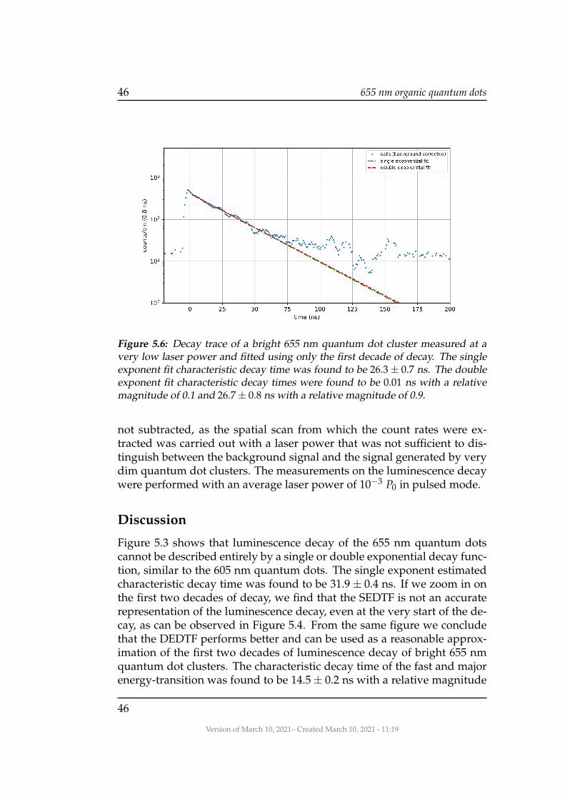
Figure 5.6: Decay trace of a bright 655 nm quantum dot cluster measured at avery low laser power and fitted using only the first decade of decay. The singleexponent fit characteristic decay time was found to be 26.3 ± 0.7 ns. The doubleexponent fit characteristic decay times were found to be 0.01 ns with a relativemagnitude of 0.1 and 26.7 ± 0.8 ns with a relative magnitude of 0.9.

not subtracted, as the spatial scan from which the count rates were ex-tracted was carried out with a laser power that was not sufficient to dis-tinguish between the background signal and the signal generated by verydim quantum dot clusters. The measurements on the luminescence decaywere performed with an average laser power of 10−3 P0 in pulsed mode.

Discussion

Figure 5.3 shows that luminescence decay of the 655 nm quantum dotscannot be described entirely by a single or double exponential decay func-tion, similar to the 605 nm quantum dots. The single exponent estimatedcharacteristic decay time was found to be 31.9 ± 0.4 ns. If we zoom in onthe first two decades of decay, we find that the SEDTF is not an accuraterepresentation of the luminescence decay, even at the very start of the de-cay, as can be observed in Figure 5.4. From the same figure we concludethat the DEDTF performs better and can be used as a reasonable approx-imation of the first two decades of luminescence decay of bright 655 nmquantum dot clusters. The characteristic decay time of the fast and majorenergy-transition was found to be 14.5 ± 0.2 ns with a relative magnitude

46



Figure 5.7: Comparison of luminescence decay of different quantum dot clusters.The position-dependent count rates are indicated in the legend.

Figure 5.8: Scatter plot of the estimated single exponential characteristic decaytimes of the measurements shown in Figure 5.7 over the position-dependentcount rate from a spatial scan.

of 0.6 and a characteristic decay time of 44.3 ± 0.3 for the slower energy-


47


transition with a relative magnitude of 0.4.

From Figure 5.4 we conclude that the SEDTF cannot be used to accuratelydescribe the first two decades of luminescence decay of 655 nm quantumdots.

From Figure 5.5 we conclude that the estimated decay rate does notdepend on the laser power, nor the received signal strength by the SPCM.We discovered that the optimization of the SEDTF on the luminescencedecay of the bright quantum dot cluster depends on the range that thefitting is applied. A fit of the SEDTF over the first two decades of decayresulted in an estimated characteristic decay time τ of 31.9 ns, whereas afit over solely the first decade of decay resulted in the estimation τ = 26.3.As the low power measurement only shows approximately one decade ofdecay before the background signal takes over, we are convinced the fitrestricted to the first decade of decay is more reliable when comparing thehigh and low power measurement.

When we applied the DEDTF fit to the first decade of decay of the lowpower measurement, we found characteristic decay times τ1 = 0.01 nswith a relative magnitude of 0.1 and τ2 = 26.7 ± 0.8 ns with a relativemagnitude of 0.9. As the major estimated characteristic decay time is verycomparable to the SEDTF decay time and has high relative magnitude, weconclude that the luminescence decay of the 655 nm quantum dot clustercan be described with a SEDTF during the first decade of decay at very lowlaser powers. It is unclear what the underlying cause is for this differencebetween the low and high laser power measurement.

From Figure 5.8 we conclude that the 655 nm quantum dots have widelydiffering characteristic decay times, ranging from τ = 2 ns up to τ = 26 nsfor the SEDTF fits on the first decade of decay. As was already stated forthe 605 nm quantum dots, brighter quantum dot clusters generally showlonger characteristic decay times. Figure 5.8 reinforces this observation.We find a positive correlation between the fluorescence signal strengthfrom a spatial scan and the estimated characteristic decay time using theSEDTF on the first decade of decay. It remains unclear what causes largerquantum dot clusters to have a slower luminescence decay.

48



5.4 Bleaching and blinking

Results

Figure 5.9 shows the gradual decrease of the fluorescence signal of a quan-tum dot cluster on Sample 12 (the medium density sample) when exposedto a continuous wave laser power of P0. The corresponding measurementhad a duration of 120 s and was performed with a laser power of P0. Thetime tagged photon events were distributed over 1 s bins. The first ∼ 5 swere measured with the laser turned off and show the background signal,resulting in the first plateau with a value of ∼ 450 counts per 1 s bin. Thenext ∼ 5 s were measured at an empty spot on the sample, measuringthe fluorescence signal generated by the sample glass, resulting in the sec-ond plateau with a value of ∼ 1300 counts per 1 s bin. After the secondplateau, the laser is focused on the quantum dot cluster. An initial signalstrength of 2 · 103 counts/s was found. Over the course of 110 s, the fluo-rescence signal strength gradually drops to 1.8 · 103 counts/s, resulting ina bleaching rate of ∼ 0.1% per second.

Figure 5.9: Time resolved dynamics of a quantum dot cluster on Sample 12. Thefirst plateau is the dark count rate of the new SPCM. The second plateau is thebackground fluorescence of the sample glass. The apparent gradual bleachingof 2 counts/s2 is surprising, as it suggests that a single quantum dot contributesvery little to the total signal strength of the quantum dot cluster during this mea-surement. We conclude that the laser beam was not focused optimally on thequantum dot cluster during the measurement, resulting in a sub-optimal signalstrength.

Figure 5.10 shows the time resolved dynamics of a fluorescence source


49


on Sample 10 (also shown on the right of Figure 5.1). The figure consistsof four concatenated, 120 s TTTR measurements of photon events thatare distributed over 0.1 s bins. The measurements were carried out witha laser power P0. Each measurement starts with ∼ 5 s of backgroundsignal, resulting in the four signal drops that can be seen in the figure.Again, the plateaus have a value of approximately 50-60 counts/bin, or500-600 counts/s, corresponding roughly to the dark count rate of the’new’ SPCM. Each plateau is followed by ∼ 5 s of recording of the flu-orescence signal from the sample glass, with a value of approximately70 counts/bin, or 700 counts/s, corresponding with the background flu-orescence signal that can be observed on the right of Figure 5.1. Afteraround 60 s, fluorescence signal that surpassed the background fluores-cence signal was observed, increasing the measured signal with a value ofof approximately 30-40 counts/bin or ∼ 300-400 counts/s. This is in agree-ment with the fluorescence signal value for the local variable of the rightspatial scan of Figure 5.1. This fluorescence signal showed up and disap-peared periodically, with periods of darkness in the order of 10-50 s. Afterthe second 120 s measurement, the fluorescence signal of a 1000 counts/swas not observed again, as can be seen in the figure.

Figure 5.10: Concatenation of the four 120s time trace measurements of the quan-tum dot on the right of Figure 5.1. Each plateau signifies the start of a new 120smeasurement. Each plateau is followed by ∼ 5 s of sample glass fluorescence.

50


5.5 Conclusions 51

Discussion

From the time trace experiments we conclude that the 655 nm quantumdots also show both blinking and bleaching behaviour, which should betaken into account during other measurements.

Quantized bleaching can be observed in Figure 5.10. After approx-imately 200 seconds of laser exposure with power P0, the fluorescencesignal of the quantum dot(s) disappeared and did not reappear duringthe following experiments. We conclude that the quantum dot(s) havebleached as a consequence of prolonged high power laser exposure.

In addition to the quantized bleaching, Figure 5.10 shows blinkingbehaviour. We observed periods of approximately 10 - 50 s of fluores-cence darkness. When the fluorescence signal reappears after a periodof darkness, it appears to return to the original signal strength of ∼ 300-400 counts/s, showing only two states.

The observation of quantized bleaching combined with the apparenttwo-state blinking behaviour convinces us that the quantum dot shown onthe right of Figure 5.1 is a single quantum dot, producing ∼ 300 detectedfluorescence photons per second at a laser power of P0.

5.5 Conclusions

Similar to the 605 nm quantum dots, the 655 nm quantum dots have widelydiffering fluorescence characteristics. In the cross sectional scans we haveobserved fluorescent sources with differing signal strength up to a factor2 · 104 and comparable FWHM sizes of ∼ 1.2 − 2 µm. We conclude thatthe actual spatial resolution has remained constant between the measure-ments on the 605 nm and 655 nm quantum dots. In addition, we concludethat the 655 nm quantum dots also have a high tendency of clustering andeven super clustering and that these clusters have a size much smallerthan the spatial resolution of the experimental setup. In contrast to theobserved clustering, it is plausible that a single quantum dot has also beenobserved on the right of Figure 5.1.

The first two decades of luminescence decay of bright 655 nm quan-tum dot clusters cannot be described accurately by a fitted SEDTF. How-ever, measurements on the same quantum dot cluster with a far lowerlaser power show luminescence decay that can be described by a SEDTFmuch better. The estimated characteristic decay time did not differ be-tween these measurements. It is unclear what causes the difference in theshape of the luminescence decay measured with high and low laser power.


51


A fit of the DEDTF on the luminescence decay of bright quantum dot clus-ters proved to be more successful, again suggesting that other, slower en-ergy transitions play a prominent role in the luminescence decay of 655nm quantum dot clusters.

The estimated characteristic decay time of the 655 nm quantum dotsdiffers widely and ranges between 2 ns and 26 ns when fitted with theSEDTF on the first decade of decay. This difference in characteristic decaytime can be observed in Figure 5.7. From Figure 5.8 we conclude that thefluorescence signal strength from a spatial scan and the estimated charac-teristic decay time are positively correlated.

Similar to the 605 nm quantum dots, the effects of bleaching and blink-ing were observed for the 655 nm quantum dots and should be taken intoaccount when conducting research. Gradual bleaching was observed andis shown in Figure 5.9, where the fluorescence signal drops with a rate of2 counts/s2. In comparison, Figure 5.10 shows instantaneous bleachingwith a signal drop of 300 counts/s. We conclude that the laser was not op-timally focused during the experiment shown in Figure 5.9. In addition tothe instantaneous signal drop, we observed two-level blinking behaviour.The combination of these two observations makes it very plausible that thematching fluorescence source is a single quantum dot. With this assump-tion, we conclude that single 655 nm quantum dots have a signal strengthof ∼ 300 counts/s when exposed to a laser power of P0.

52


Chapter 6Concluding discussion

Chapter 4 and 5 discuss the results of research on the fluorescence prop-erties of 605 nm and 655 nm colloidal quantum dots respectively. Bothtypes of quantum dots were investigated using the same methods. Thischapter aims to compare the conclusions of both chapters and to give anoverall conclusion on the general fluorescence characteristics of both typesof quantum dots.

In general, spatial scans show a high tendency of clustering for both thehigh density samples and the low density samples. We determined thespatial resolution of the confocal setup by analyzing the FWHM of localmaxima of fluorescence signal of different magnitudes. We found that theFWHM does not depend on the signal strength of the local maxima andconclude that the size of the imaged quantum dot clusters is much smallerthan the spatial resolution of the setup. Both type of quantum dots showhigh diversity in cluster brightness, with signal strength differing up toa factor 5000 between clusters on the high density samples and clusterson the low density samples. If we assume that the measured fluorescenceintensity of a cluster is proportional to the number of quantum dots in thegiven cluster, we find high variation in the number of quantum dots thatare located in the observed clusters. The background fluorescence signal of∼ 800− 1200 counts/s generated by the sample glass was a limiting factorin the detection of single quantum dots. A single quantum dot has beendetected in the case of 655 nm quantum dots, with an estimated signalstrength of ∼ 300 counts/s when exposed to a laser power of P0 ≈ 1 mW.

The luminescence decay of both types quantum dots was found to dif-fer widely and to be correlated to the number of quantum dots in a quan-tum dot cluster. Characteristic decay times have been estimated by fittinga single exponent decay template function to the data. The estimated de-


53

54 Concluding discussion

cay times differed between 6 ns and 20 ns for the 605 nm quantum dotsand 2 ns and 26 ns for the 655 nm quantum dots. Both types of quantumdots show exponential decay that cannot entirely be described by a singleexponent decay function. Only the first two decades of decay of bright 605nm quantum dot clusters can be approximated by the single exponent de-cay template function, whereas even the first decade of decay of bright 655nm quantum dot clusters cannot be approximated in this way. However,when bright 655 nm quantum dot clusters were measured with a very lowlaser power, the luminescence decay could be described by a single expo-nent decay function. In contrast to the shape of the decay, the estimatedcharacteristic decay time remained constant. It remains unclear why theshape of the luminescent decay changes with the provided laser power.

A double exponent decay function proved to be a better approximationof the observed behaviour, but is only able to reasonably describe the firsttwo decades of decay for both types of quantum dots. We conclude thatboth types of quantum dots show other, slower energy transitions thatplay a non-negligible role in the luminescence decay.

The effect of blinking and bleaching have been observed for the twotypes of quantum dots. Both 605 nm and 655 nm quantum dot clusterson the high density samples show a gradual decrease of fluorescence overtime when exposed to a maximum laser power of P0. This effect of bleach-ing has also been observed to occur in a more quantized way, where thesignal appears to decrease in steps of 250 counts/s in the case of 605 nmquantum dots. In the case of the 655 nm quantum dots, a sudden andpermanent drop of fluorescence signal of 300 counts/s to the backgroundfluorescence level was observed. Based on the similarity of these drops influorescence signal, we make the tentative assumption that single quan-tum dots have a fluorescence signal strength of ∼ 300 counts/s in thissetup when exposed to a laser power of P0 ≈ 1 mW.

The effect of blinking was only encountered when investigating dimquantum dot clusters. These small ensembles of quantum dots showedsudden temporary periods of lower or non-existent fluorescence signal ontime scales of 0.1 seconds up to tens of seconds. This blinking behaviourcan also be observed indirectly in the spatial scans, where sources of fluo-rescence seem to be stretched in the x-direction.

In conclusion, we do not recommend the use of these quantum dots forsimilar or follow-up research, as the fluorescence properties differ widelyand because the quantum dots are very susceptible to the effects of bleach-ing and blinking.

54


Chapter 7Appendix

7.1 Python measurement UI

With the use of the TKinter module for python, a UI class was developedto facilitate the measurement process. Figures 7.1, 7.2 and 7.3 show thedifferent windows of the UI. Figure 7.3 shows the main window of the UI.

On the left of the main window spatial scans can be executed. Thefields ’start x pos’ and ’start y pos’ take values between 0 and 100 and setthe starting coordinates of the spatial scan. The field ’distance’ is used toset the scanning distance for both the x and y direction (be cautious withthis input value, as the PI-E517 has a maximum range of ∼ 100 µm). The’steps’ field controls the amount of measurements steps taken to traversethe scanning distance. The amount of data points therefore is steps2. Thebuttons below are self-explanatory.

To the right of the scanning menu, we find a menu that is loosely re-lated to saturation measurement. The three upper fields can be used to setthe position of the PI-E517 by entering the coordinates and pressing the’set piezo position’ button on the right of the window. The buttons beloware self-explanatory. One important button is the ’set min attenuator volt-age’ button and its matching input field right below. This can be used toset the maximum laser power when performing any other measurement.A higher voltage means a lower laser power, with a voltage ranging from0 to 5 volts.

To the right of the saturation menu, a bleaching measurement menu isfound. These function were rarely used and need more testing.

All the way to the right the general options can be found. The differentfunctions are explained in Table 7.1.


55

56 Appendix

button functioncreate new experiment opens the experiment naming prompt

and creates a new experiment direc-tory. All measurements performed af-ter this action will be stored in thisnew directory.

exit program sets the laser power to 0 (in order toprevent bleaching) and terminates theprogram.

call custom function executes a custom function which canbe added to the python ode.

set piezo position sets the position of the PI-E517 tothe coordinates entered in the coordi-nates field above the ’start saturation’button.

get current piezo position prints the current position of the PI-E517 to the console.

get current count rate measures and prints the photon countrate at the current position.

max laser power sets the attenuator voltage to thevalue set by the ’set min attenuatorvoltage’ button (default value is 0).

min laser power sets the attenuator voltage to 5 volts(turns off the laser).

get current laser power estimates the power on the samplebased on the voltage reading of thephotodiode (see Table 3.1.) and printsit to the console.

optimize z position scans the z-position of the PI-E517 onthe currect x and y position and re-turns a graph with the resulting countrate for each z-position. This funtioncan be used to optimize the z-positionof the setup (see Section 3.3).

Table 7.1: General functions of the UI menu.

56


7.1 Python measurement UI 57

Figure 7.1: Starting screen of the measurement UI. The user can input the nameof the experiment directory all the measurement data and figures will be storedin. The directory name will automatically be prefixed by a date tag.

Figure 7.2: Second screen of the measurement UI. The user can choose where theexperiment folder is stored.

The UI is by no means finished and bug-free, and should be testedand tweaked thoroughly before it can be used for follow-up research. ThePython code is provided below.


57

58 Appendix

Figure 7.3: Main measurement UI.

# −*− c o d i n g : u t f −8 −*−# a u t h o r : Matt van den Nieuwenhui jzen , mat tvdn i euwenhui j z en@gmai l . com

import t k i n t e r as tkfrom t k i n t e r import f i l e d i a l o gfrom t k i n t e r import s impledialogfrom datetime import dateimport osimport FLEXperiments as EXPimport timeimport numpy as npimport m a t p l o t l i b . pyplot as p l t

# Func t i on t h a t a s s i g n s w i d g e t s t o a window g r i d b a s e d on t y p edef SetWidgets ( l s t ) :

index=0for i in l s t :

i f i s i n s t a n c e ( i , tk . Label ) :i . gr id ( row=index , column=1 , s t i c k y =”w” )

e l i f i s i n s t a n c e ( i , tk . Button ) :i . gr id ( row=index , column=0 , s t i c k y = ’nsew ’ )index +=1

e lse :i . gr id ( row=index , column=0 , s t i c k y = ’ e ’ )index +=1

return

c l a s s ExpManager ( ) :”””ExpManager c r e a t e s a b r i d g e be tween t h e UI and t h e d i f f e r e n tmeasurement c l a s s e s and f u n c t i o n s .”””

#TODO: p r i n t t ime i n d i c a t i o n s#TODO: s a v e f i l e s o f z s can#TODO: power management with a t t e n u a t o r#TODO: f i x s i z e d i f f e r e n c e be tween scan p l o t s

def i n i t ( s e l f ) :

s e l f . e x p f o l d e r = ”C:/ Users/ l i o n /Documents/Matt BRP python/DATA/datadump”

58



s e l f . Scan = EXP . XYScan ( path= s e l f . e x p f o l d e r )s e l f . Sat = EXP . S a t u r a t i o n ( )s e l f . Bleach = EXP . Bleaching ( )

s e l f . CreateExpFolder ( )

s e l f . polmax = 0s e l f . polmin = 5

s e l f . PDzero = s e l f . Sat . GetPower ( )s e l f . SetPolar izerMin ( )return

def CreateExpFolder ( s e l f ) :”””Asks t h e u s e r f o r a pa th where t h e d a t a o f t h i s s e s s i o n s h o u l d be s a v e d .”””

input window = tk . Tk ( )input window . withdraw ( )exp name = simpledialog . a s k s t r i n g ( ” Input ” , ” Create new experiment : ” ,

parent=input window )

f o l d e r p i c k e r = tk . Tk ( )f o l d e r p i c k e r . withdraw ( )f i l e p a t h = f i l e d i a l o g . a s k d i r e c t o r y ( )

today = date . today ( ) . s t r f t i m e ( ”%Y%m%d” )

s e l f . e x p f o l d e r = ”/ ” . format ( f i l e p a t h , today , exp name )s e l f . Scan . path = s e l f . e x p f o l d e r

i f ( not os . path . e x i s t s ( s e l f . e x p f o l d e r ) ) : os . mkdir ( s e l f . e x p f o l d e r )input window . destroy ( )f o l d e r p i c k e r . destroy ( )return

def SetPolAngle ( s e l f ) :value = max ( min ( f l o a t ( ent po langle . get ( ) ) , 5 ) , 0 )s e l f . polmax = valueprint ( ” a t t e n u a t o r vol tage s e t to V” . format ( value ) )return

def GetPower ( s e l f ) :print ( ” l a s e r power i s watts ” . format ( s e l f . Sat . GetPower ( ) − s e l f . PDzero ) )

def OptimizeZ ( s e l f ) :# t o d o r e s e t z p o s i t i o ns e l f . SetPolarizerMax ( )s e l f . Scan . ZScan ( s e l f . e x p f o l d e r )s e l f . SetPolar izerMin ( )

def SaveScan ( s e l f ) :s e l f . Scan . SaveData ( s e l f . e x p f o l d e r )return

def PlotScan ( s e l f ) :


59

60 Appendix

s e l f . Scan . PlotData ( )s e l f . Scan . PlotData ( lower l im =100 , upper lim =3000 , l i n e a r =True )s e l f . Scan . PlotData ( lower l im =100 , upper lim =1000 , l i n e a r =True )s e l f . Scan . PlotData ( lower l im=None , upper lim=None , l i n e a r =True )return

def MakeScan ( s e l f ) :s e l f . SetPolarizerMax ( )s t a r t p o s = [ f l o a t ( e n t y s t a r t . get ( ) ) , f l o a t ( e n t x s t a r t . get ( ) ) ]d i s t a n c e = f l o a t ( e n t s c a n d i s t a n c e . get ( ) )s t eps = i n t ( e n t s c a n s t e p s . get ( ) )

print ( ” s t a r t i n g scan ” )s e l f . GetPower ( )

s e l f . Scan . Scan ( s t a r tp o s , dis tance , s teps )s e l f . SetPolar izerMin ( )s e l f . PlotScan ( )return

def S e t P o s i t i o n ( s e l f ) :x = ent xcoord . get ( )y = ent ycoord . get ( )z = ent zcoord . get ( )s e l f . Scan . SetXY ( y , x )s e l f . Scan . SetZ ( z )print ( ” p o s i t i o n s e t ! ” )return

def GetPos i t ion ( s e l f ) :p o s i t i o n = s e l f . Scan . ReturnCurrentPiezoPosi t ion ( )print ( ” current p o s i t i o n : ” )print ( p o s i t i o n )return p o s i t i o n

def GetCountRate ( s e l f ) :s e l f . SetPolarizerMax ( )time . s leep ( 2 )print ( ” count r a t e a t current p o s i t i o n ” )print ( s e l f . Scan . ReturnCountRate ( autoDisable=True ) )s e l f . SetPolar izerMin ( )return

def MeasureSaturation ( s e l f ) :s e l f . SetPolarizerMax ( )s e l f . Sat . MeasureSaturation ( s e l f . e x p f o l d e r )s e l f . SetPolar izerMin ( )

def SetPolarizerMax ( s e l f ) :s e l f . Sat . Se tPolar izerAngle ( s e l f . polmax )

def SetPolar izerMin ( s e l f ) :s e l f . Sat . Se tPolar izerAngle ( s e l f . polmin )

def BleachExp ( s e l f ) :

60



s e l f . SetPolarizerMax ( )time = f l o a t ( ent b leacht ime . get ( ) )s teps = i n t ( e n t b l e a c h s t e p s . get ( ) )s e l f . Bleach . MeasureBleaching ( time , steps , s e l f . GetPos i t ion ( ) )s e l f . SetPolar izerMin ( )return

def PlotB leach ( s e l f ) :s e l f . Bleach . PlotData ( )return

def SaveBleach ( s e l f ) :s e l f . Bleach . SaveData ( )return

def d e l ( s e l f ) :s e l f . SetPolar izerMin ( )del s e l f . Satdel s e l f . Scandel s e l f . Bleachwindow . destroy ( )

Experiment = ExpManager ( )

# ======================================================# TKINTER WINDOWS# ======================================================

window = tk . Tk ( )window . t i t l e ( ” Experiment Manager” )window . r e s i z a b l e ( width=False , height=Fa l se )

entryWidth = 5

# ======================================================# scan s e c t i o n# ======================================================frame scan = tk . Frame ( )

scan i tems = [l b l x s t a r t := tk . Label ( master=frame scan , t e x t =” s t a r t x pos” ) ,e n t x s t a r t := tk . Entry ( master=frame scan , width=entryWidth ) ,

l b l y s t a r t := tk . Label ( master=frame scan , t e x t =” s t a r t y pos” ) ,e n t y s t a r t := tk . Entry ( master=frame scan , width=entryWidth ) ,

l b l s c a n d i s t a n c e := tk . Label ( master=frame scan , t e x t =” d i s t a n c e ” ) ,e n t s c a n d i s t a n c e := tk . Entry ( master=frame scan , width=entryWidth ) ,

l b l s c a n s t e p s := tk . Label ( master=frame scan , t e x t =” s teps ” ) ,e n t s c a n s t e p s := tk . Entry ( master=frame scan , width=entryWidth ) ,

btn scan := tk . Button ( master=frame scan , t e x t =” s t a r t xy−scan ” , command=Experiment. MakeScan ) ,

b t n p l o t s c := tk . Button ( master=frame scan , t e x t =” p l o t l a s t xy−scan ” , command=


61

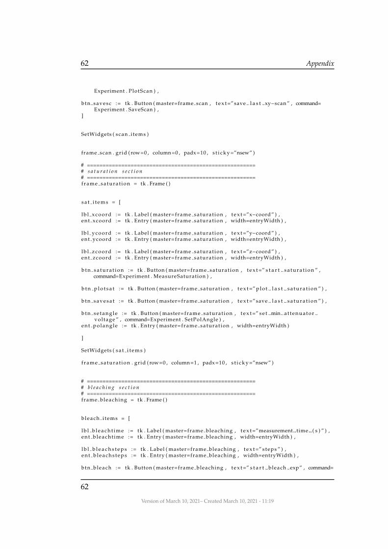
62 Appendix

Experiment . PlotScan ) ,

b tn savesc := tk . Button ( master=frame scan , t e x t =” save l a s t xy−scan ” , command=Experiment . SaveScan ) ,

]

SetWidgets ( scan i tems )

frame scan . gr id ( row=0 , column=0 , padx=10 , s t i c k y =”nsew” )

# ======================================================# s a t u r a t i o n s e c t i o n# ======================================================f r a m e s a t u r a t i o n = tk . Frame ( )

s a t i t e m s = [

l b l x c o o r d := tk . Label ( master=frame saturat ion , t e x t =”x−coord ” ) ,ent xcoord := tk . Entry ( master=frame saturat ion , width=entryWidth ) ,

l b l y c o o r d := tk . Label ( master=frame saturat ion , t e x t =”y−coord ” ) ,ent ycoord := tk . Entry ( master=frame saturat ion , width=entryWidth ) ,

l b l z c o o r d := tk . Label ( master=frame saturat ion , t e x t =”z−coord ” ) ,ent zcoord := tk . Entry ( master=frame saturat ion , width=entryWidth ) ,

b t n s a t u r a t i o n := tk . Button ( master=frame saturat ion , t e x t =” s t a r t s a t u r a t i o n ” ,command=Experiment . MeasureSaturation ) ,

b t n p l o t s a t := tk . Button ( master=frame saturat ion , t e x t =” p l o t l a s t s a t u r a t i o n ” ) ,

b t n s a v e s a t := tk . Button ( master=frame saturat ion , t e x t =” save l a s t s a t u r a t i o n ” ) ,

b t n s e t a n g l e := tk . Button ( master=frame saturat ion , t e x t =” s e t min a t t e n u a t o rvol tage ” , command=Experiment . SetPolAngle ) ,

en t po langle := tk . Entry ( master=frame saturat ion , width=entryWidth )

]

SetWidgets ( s a t i t e m s )

f r a m e s a t u r a t i o n . gr id ( row=0 , column=1 , padx=10 , s t i c k y =”nsew” )

# ======================================================# b l e a c h i n g s e c t i o n# ======================================================f rame bleaching = tk . Frame ( )

b leach i tems = [

l b l b l e a c h t i m e := tk . Label ( master=frame bleaching , t e x t =”measurement time ( s ) ” ) ,ent b leacht ime := tk . Entry ( master=frame bleaching , width=entryWidth ) ,

l b l b l e a c h s t e p s := tk . Label ( master=frame bleaching , t e x t =” s teps ” ) ,e n t b l e a c h s t e p s := tk . Entry ( master=frame bleaching , width=entryWidth ) ,

b tn bleach := tk . Button ( master=frame bleaching , t e x t =” s t a r t bleach exp” , command=

62



Experiment . BleachExp ) ,

b t n p l o t b l e a c h := tk . Button ( master=frame bleaching , t e x t =” p l o t l a s t bleach exp” ) ,

b tn savebleach := tk . Button ( master=frame bleaching , t e x t =” save l a s t bleach exp” )]

SetWidgets ( b leach i tems )

frame bleaching . gr id ( row=0 , column=2 , padx=10 , s t i c k y =”nsew” )

# ======================================================# g e n e r a l o p t i o n s# ======================================================

f rame general = tk . Frame ( )

ge ner a l i t ems = [b t n s e t p a t h := tk . Button ( master=frame general , t e x t =” c r e a t e new experiment ” ,

command=Experiment . CreateExpFolder ) ,b t n e x i t := tk . Button ( master=frame general , t e x t =” e x i t program” , command=

Experiment . d e l ) ,btn customfunct ion := tk . Button ( master=frame general , t e x t =” c a l l custom funct ion ”

) ,

b t n s e t p o s i t i o n := tk . Button ( master=frame general , t e x t =” s e t piezo p o s i t i o n ” ,command=Experiment . S e t P o s i t i o n ) ,

b t n g e t p o s i t i o n := tk . Button ( master=frame general , t e x t =” get current piezop o s i t i o n ” , command=Experiment . GetPos i t ion ) ,

b tn getcount := tk . Button ( master=frame general , t e x t =” get current count r a t e ” ,command=Experiment . GetCountRate ) ,

bnt setpolmax := tk . Button ( master=frame general , t e x t =”max l a s e r power” , command=Experiment . SetPolarizerMax ) ,

bnt setpolmin := tk . Button ( master=frame general , t e x t =”min l a s e r power” , command=Experiment . SetPolar izerMin ) ,

bnt getpower := tk . Button ( master=frame general , t e x t =” get current l a s e r power” ,command=Experiment . GetPower ) ,

bnt opt imizez := tk . Button ( master=frame general , t e x t =” optimize z p o s i t i o n ” ,command=Experiment . OptimizeZ ) ,

]

SetWidgets ( ge ne ra l i t ems )

frame general . gr id ( row=0 , column=3 , padx=10 , s t i c k y =”nsew” )

# Run t h e a p p l i c a t i o nwindow . mainloop ( )


63

64 Appendix

7.2 Python measurement classes

Below, the python code that was used to control the different devices fromthe experimental setup is shown. It consists of 3 classes. The XYScan classholds all actions and data related to spatial scanning of the fluorescencesignal and can be used to set the position of the piezo controller with thefunctions SetXY and SetZ. The Bleaching class holds all actions and datarelated to a bleaching measurement. This class was rarely used, as a timetrace with the use of the th260 software proved to be a more useful methodof observing bleaching. Finally, the Saturation class holds all actions anddata related to saturation measurements. This class can also be used to setand measure the current laser power with the functions SetPolarizerAngle(this name is deprecated since the laser power controlling polarizer waslater replaced by a voltage controlled optical attenuator) and GetPower.

# −*− c o d i n g : u t f −8 −*−# a u t h o r : Matt van den Nieuwenhui jzen , mat tvdn i euwenhui j z en@gmai l . com

from PIpiezo import E517from th260 master import th260 as THimport numpy as npimport timeimport mathimport m a t p l o t l i b . pyplot as p l timport t h o r l a b s a p t as apt

import nidaqmx as dxfrom nidaqmx . cons tants import Edgefrom nidaqmx . cons tants import Acquisit ionTypefrom nidaqmx import s t r e a m w r i t e r s

import Analyt i cs as AL

# Minimal t i m e d e l a y be tween c o n s e c u t i v e measurements o f a d e v i c eTimeHarpSleep = 0 . 1 5piezoSleep = 0 . 1

# Deadtime o f t h e s p cDEADTIME = 40e−9

# Upper and l o w e r l i m i t o f count r a t e range o f t h e th260 APITH upper=np . log10 (5 e5 )TH lower=np . log10 (8 e1 )

# r e t u r n s a t imes tampdef TimeStamp ( ) :

return s t r ( i n t ( time . time ( ) ) )

# c o r r e c t s t h e count r a t e b a s e d on d e a d t i m edef CountCorrection ( countra te ) :

return (1/(1 −DEADTIME* countra te ) ) * countra te

# ==========================================================

64


7.2 Python measurement classes 65

# XYSCAN# ==========================================================

c l a s s XYScan ( ) :”””XYScan manages a l l a c t i o n s t h a t a r e r e l a t e d t o s c a n s o f t h e sample .”””

# TODO: SPC dead −t ime count r a t e c o r r e c t i o n# TODO: f i x l i m i t s o f p l o t s# TODO: s a v e v a l u e s o f z s can

def i n i t ( s e l f , path ) :s e l f . Piezo = E517 . E517 ( )

s e l f . TimeHarp = TH. TH260 (TH. g e t a v i l a b l e d e v i c e s ( ) [ 0 ] )

s e l f . xCoords = [ ]s e l f . yCoords = [ ]s e l f . counts = [ ]

s e l f . maxima = [ ]

s e l f . timeStamp = 0

s e l f . zcoord = 0

s e l f . s t a r t p o s = 0s e l f . d i s t a n c e = 100s e l f . s t eps = 10

s e l f . Figure = Nones e l f . Ax = None

# I f t r u e more i n f o r m a t i o n i s p r i n t e d dur ing t h e e x p e r i m e n t ss e l f . debug = Trues e l f . path = path

print ( ”XYScan i n i t i a l i s e d ” )return

def EnableTH ( s e l f ) :s e l f . TimeHarp . openDevice ( )s e l f . TimeHarp . i n i t i a l i z e ( s e t t i n g s = ’mode ’ : 2 )

def DebugMode( s e l f , mode) :# T og g l e debug modei f (mode) : s e l f . debug = Truee lse : s e l f . debug = Fa lse

def ZScan ( s e l f , path ) :# TODO: f i x f i r s t p o i n t o f measurement ?

c u r r e n t p o s i t i o n = s e l f . ReturnCurrentPiezoPosi t ion ( )s e l f . EnableTH ( )

# t h e f i r s t measurement i s a lways o f f f o r some r e a s o n . . .= s e l f . ReturnCountRate ( )

p o s i t i o n s = np . arange ( 0 , 100 , 0 . 5 )counts = np . empty ( p o s i t i o n s . shape )


65

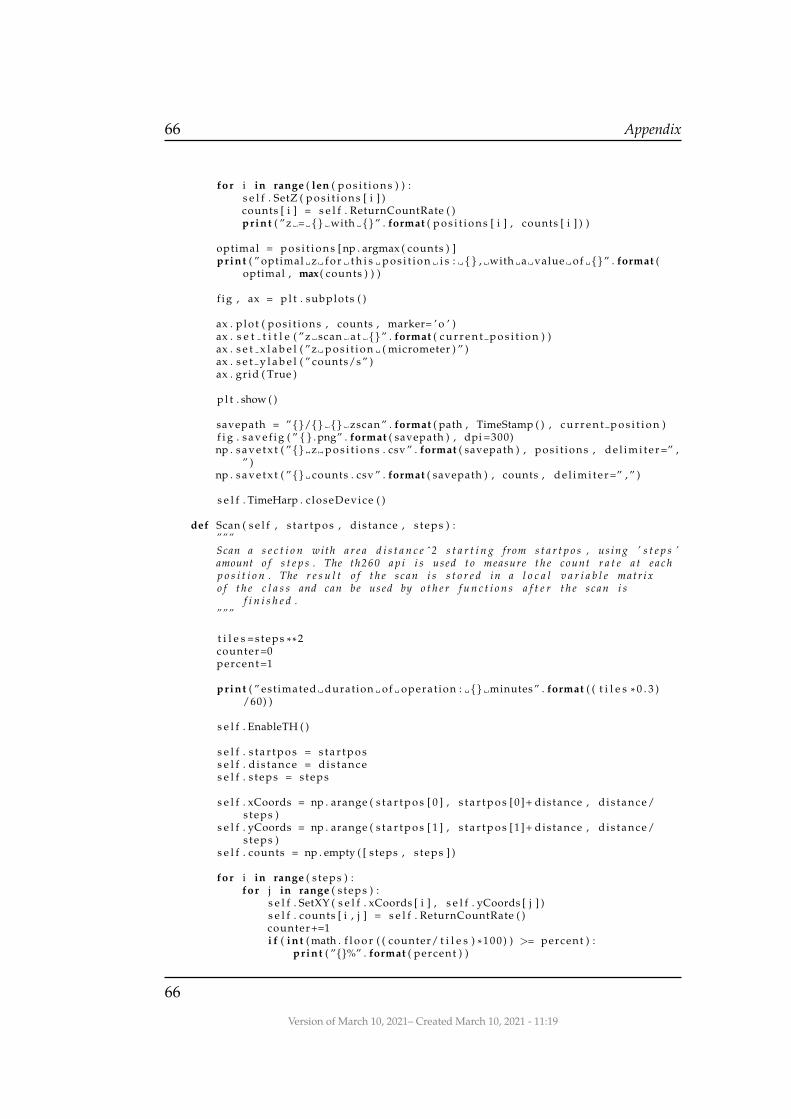
66 Appendix

for i in range ( len ( p o s i t i o n s ) ) :s e l f . SetZ ( p o s i t i o n s [ i ] )counts [ i ] = s e l f . ReturnCountRate ( )print ( ”z = with ” . format ( p o s i t i o n s [ i ] , counts [ i ] ) )

optimal = p o s i t i o n s [ np . argmax ( counts ) ]print ( ” optimal z f o r t h i s p o s i t i o n i s : , with a value of ” . format (

optimal , max ( counts ) ) )

f ig , ax = p l t . subplots ( )

ax . p l o t ( pos i t ions , counts , marker= ’ o ’ )ax . s e t t i t l e ( ”z scan at ” . format ( c u r r e n t p o s i t i o n ) )ax . s e t x l a b e l ( ”z p o s i t i o n ( micrometer ) ” )ax . s e t y l a b e l ( ” counts/s ” )ax . gr id ( True )

p l t . show ( )

savepath = ”/ zscan ” . format ( path , TimeStamp ( ) , c u r r e n t p o s i t i o n )f i g . s a v e f i g ( ” . png” . format ( savepath ) , dpi =300)np . s a v e t x t ( ” z p o s i t i o n s . csv ” . format ( savepath ) , pos i t ions , d e l i m i t e r =” ,

” )np . s a v e t x t ( ” counts . csv ” . format ( savepath ) , counts , d e l i m i t e r =” , ” )

s e l f . TimeHarp . c loseDevice ( )

def Scan ( s e l f , s t a r t p o s , dis tance , s teps ) :”””Scan a s e c t i o n with a r e a d i s t a n c e ˆ2 s t a r t i n g from s t a r t p o s , us ing ’ s t e p s ’amount o f s t e p s . The th260 a p i i s used t o measure t h e count r a t e a t e a c hp o s i t i o n . The r e s u l t o f t h e scan i s s t o r e d in a l o c a l v a r i a b l e mat r i xo f t h e c l a s s and can be used by o t h e r f u n c t i o n s a f t e r t h e s can i s

f i n i s h e d .”””

t i l e s =s teps * * 2counter =0percent =1

print ( ” est imated duration of operat ion : minutes ” . format ( ( t i l e s * 0 . 3 )/60) )

s e l f . EnableTH ( )

s e l f . s t a r t p o s = s t a r t p o ss e l f . d i s t a n c e = d i s t a n c es e l f . s t eps = s teps

s e l f . xCoords = np . arange ( s t a r t p o s [ 0 ] , s t a r t p o s [ 0 ]+ dis tance , d i s t a n c e/s teps )

s e l f . yCoords = np . arange ( s t a r t p o s [ 1 ] , s t a r t p o s [ 1 ]+ dis tance , d i s t a n c e/s teps )

s e l f . counts = np . empty ( [ steps , s teps ] )

for i in range ( s t eps ) :for j in range ( s teps ) :

s e l f . SetXY ( s e l f . xCoords [ i ] , s e l f . yCoords [ j ] )s e l f . counts [ i , j ] = s e l f . ReturnCountRate ( )counter+=1i f ( i n t ( math . f l o o r ( ( counter/ t i l e s ) * 1 0 0 ) ) >= percent ) :

print ( ”%” . format ( percent ) )

66



percent +=1

print ( ”” )print ( ”Scan completed ! ” )# s e l f . maxima = AL . FindLocalMaxima ( s e l f . c o u n t s )# s e l f . maxima [ : , 0 ] = s e l f . s t a r t p o s [0 ] + s e l f . maxima * ( s e l f . d i s t a n c e / s e l f .

s t e p s )# s e l f . maxima [ : , 1 ] = s e l f . s t a r t p o s [1 ] + s e l f . maxima * ( s e l f . d i s t a n c e / s e l f .

s t e p s )

# p r i n t (” l o c a l maxima found a t : ” )# p r i n t ( s e l f . maxima )

s e l f . timeStamp = TimeStamp ( )

s e l f . TimeHarp . c loseDevice ( )return

def SetXY ( s e l f , xCoord , yCoord ) :”””S e t s t h e x and y p o s i t i o n o f t h e PI c o n t r o l l e r .”””s e l f . Piezo . s e t p o s i t i o n ( x=yCoord , y=None , z=xCoord )time . s leep ( piezoSleep )return

def SetZ ( s e l f , zCoord ) :”””S e t t h e z p o s i t i o n o f t h e PI c o n t r o l l e r . I n c r e a s i n g t h e z w i l li n c r e a s e t h e d i s t a n c e be tween t h e sample and t h e o b j e c t i v e .( t h i s n e e d s t o be c h e c k e d ! )”””

s e l f . Piezo . s e t p o s i t i o n ( x=None , y=zCoord , z=None )time . s leep ( piezoSleep )s e l f . zcoord = zCoordreturn

def ReturnCurrentPiezoPosi t ion ( s e l f ) :”””Asks t h e PI c o n t r o l l e r f o r i t s c u r r e n t p o s i t i o n s and r e t u r n s t h e r e s u l t .”””posDic = s e l f . Piezo . g e t p o s i t i o n ( )return [ posDic [ ’X ’ ] , posDic [ ’Y ’ ] , posDic [ ’Z ’ ] ]

def PlotData ( s e l f , lower l im=TH lower , upper lim=TH upper , l i n e a r =False ,c o l o r = p l t . cm . j e t ) :”””P l o t t h e r e s u l t s o f t h e l a s t s can us ing a l o g a r i t h m i c h e a t map .”””

i f ( s e l f . xCoords . s i z e == 0 or s e l f . yCoords . s i z e == 0 or s e l f . counts . s i z e== 0) :print ( ”No data a v a i l a b l e ” )return

s e l f . Figure , s e l f . Ax = p l t . subplots ( )


67

68 Appendix

s e l f . Figure . s e t s i z e i n c h e s ( 9 , 5 , forward=True )

i f ( l i n e a r ) :counts = s e l f . countstag = ’ l i n ’

e lse :counts = np . log10 ( s e l f . counts )tag = ’ log10 ’

im = s e l f . Ax . pcolor ( s e l f . yCoords , s e l f . xCoords , counts , vmin=lower lim ,vmax=upper lim , shading= ’ n e a r e s t ’ , cmap= c o l o r )

s e l f . Ax . s e t x l a b e l ( ”x p o s i t i o n ( micrometer ) ” )s e l f . Ax . s e t y l a b e l ( ”y p o s i t i o n ( micrometer ) ” )s e l f . Ax . gr id ( True , c o l o r =” black ” , lw = 0 . 5 )cb = s e l f . Figure . c o l or ba r ( im , ax= s e l f . Ax)cb . s e t l a b e l ( ” log ( counts/s ) ” , r o t a t i o n =270 , labelpad =15)s e l f . Ax . s e t a s p e c t ( ” equal ” )s e l f . Ax . s e t t i t l e ( ” counts/s per pos i t ion , z=” . format ( s e l f .

ReturnCurrentPiezoPosi t ion ( ) [ 1 ] ) )p l t . show ( )

savepath = ”/” . format ( s e l f . path , s e l f . timeStamp )

s e l f . Figure . s a v e f i g ( ” xy−scan − .png” . format ( savepath , tag ,lower lim , upper lim ) , dpi =300)

return

def SaveData ( s e l f , path ) :”””Save t h e d a t a o f t h e l a s t s can t o a g i v e n pa th in c s v f o r m a t .”””

i f ( s e l f . Figure == None ) : s e l f . PlotData ( )savepath = ”/” . format ( path , s e l f . timeStamp )np . s a v e t x t ( ” x . csv ” . format ( savepath ) , s e l f . xCoords , d e l i m i t e r =” , ” )np . s a v e t x t ( ” y . csv ” . format ( savepath ) , s e l f . yCoords , d e l i m i t e r =” , ” )np . s a v e t x t ( ” counts . csv ” . format ( savepath ) , s e l f . counts , d e l i m i t e r =” , ” )return

def ReturnCountRate ( s e l f , autoDisable=Fa l se ) :”””Return t h e measured count r a t e o f t h e TH a t t h e c u r r e n t p o s i t i o n .”””

i f ( autoDisable ) : s e l f . EnableTH ( )counts = s e l f . TimeHarp . getCountRate ( channel =0)time . s leep ( TimeHarpSleep )i f ( autoDisable ) : s e l f . TimeHarp . c loseDevice ( )return counts

def d e l ( s e l f ) :s e l f . TimeHarp . c loseDevice ( )

# ==========================================================# BLEACHING# ==========================================================

68



c l a s s Bleaching ( ) :”””B l e a c h i n g manages a l l a c t i o n s t h a t a r e r e l a t e d t o a b l e a c h i n g e x p e r i m e n t .”””

# TODO: enhance p l o t t i n g

def i n i t ( s e l f ) :s e l f . TimeHarp = TH. TH260 (TH. g e t a v i l a b l e d e v i c e s ( ) [ 0 ] )

s e l f . timeArray = [ ]s e l f . counts = [ ]

s e l f . Figure = Nones e l f . Ax = None

s e l f . P o s i t i o n = [ ]return

def EnableTH ( s e l f ) :s e l f . TimeHarp . openDevice ( )s e l f . TimeHarp . i n i t i a l i z e ( s e t t i n g s = ’mode ’ : 2 )return

def ReturnCountRate ( s e l f , autoDisable=Fa l se ) :i f ( autoDisable ) : s e l f . EnableTH ( )counts = s e l f . TimeHarp . getCountRate ( channel =0)time . s leep ( TimeHarpSleep )i f ( autoDisable ) : s e l f . TimeHarp . c loseDevice ( )return counts

def MeasureBleaching ( s e l f , seconds , steps , p o s i t i o n ) :”””For a d u r a t i o n o f x s e conds , a y amount o f t i m e s t h e count r a t e i smeasured a t a g i v e n p o s i t i o n . I f b l e a c h i n g i s o c c u r i n g , a d e c r e a s e incount r a t e i s e x p e c t e d t o be s e e n o v e r t ime . The r e s u l t i s s t o r e d ina l o c a l v a r i a b l e f o r l a t e r use .”””

s e l f . EnableTH ( )s e l f . P o s i t i o n = p o s i t i o n

s e l f . timeArray = np . arange ( 0 , seconds , seconds/s teps )s e l f . counts = np . empty ( s teps )

for i in range ( s t eps ) :s e l f . counts [ i ] = s e l f . ReturnCountRate ( )time . s leep ( seconds/s teps )print ( ” seconds to go” . format ( seconds − i * ( seconds/s teps ) ) )

s e l f . PlotData ( )s e l f . TimeHarp . c loseDevice ( )return

def PlotData ( s e l f ) :”””P l o t t h e r e s u l t s o f t h e l a s t b l e a c h i n g e x p e r i m e n t .”””


69

70 Appendix

s e l f . Figure , s e l f . Ax = p l t . subplots ( )im = s e l f . Ax . p l o t ( s e l f . timeArray , s e l f . counts , ’ r+ ’ )s e l f . Ax . s e t x l a b e l ( ” time ( s ) ” )s e l f . Ax . s e t y l a b e l ( ” counts ” )s e l f . Ax . s e t t i t l e ( ” counts over time at ” . format ( s e l f . P o s i t i o n ) )p l t . show ( )return

def SaveData ( s e l f , path ) :i f ( s e l f . Figure == None ) : s e l f . PlotData ( )savepath = ”/ ” . format ( path , TimeStamp ( ) , s e l f . P o s i t i o n )s e l f . Figure . s a v e f i g ( ” bleaching . png” . format ( savepath ) , dpi =300)np . s a v e t x t ( ” time . csv ” . format ( savepath ) , s e l f . timeArray , d e l i m i t e r =” , ” )np . s a v e t x t ( ” counts . csv ” . format ( savepath ) , s e l f . counts , d e l i m i t e r =” , ” )return

# ==========================================================# SATURATION# ==========================================================

c l a s s S a t u r a t i o n ( ) :

# TODO: a c c u r a t e v o l t a g e t o power c o n v e r s i o n# TODO: implement s a t u r a t i o n measurement# TODO: l i m i t sample e x p o s i t i o n t o h igh power

def i n i t ( s e l f ) :s e l f . TimeHarp = TH. TH260 (TH. g e t a v i l a b l e d e v i c e s ( ) [ 0 ] )

s e l f . powers = Nones e l f . counts = None

def EnableTH ( s e l f ) :s e l f . TimeHarp . openDevice ( )s e l f . TimeHarp . i n i t i a l i z e ( s e t t i n g s = ’mode ’ : 2 )return

def ReturnCountRate ( s e l f , autoDisable=Fa l se ) :i f ( autoDisable ) : s e l f . EnableTH ( )counts = s e l f . TimeHarp . getCountRate ( channel =0)time . s leep ( TimeHarpSleep )i f ( autoDisable ) : s e l f . TimeHarp . c loseDevice ( )return counts

def MeasureSaturation ( s e l f , path , s teps =100) :s e l f . EnableTH ( )

vo l tages = np . l i n s p a c e ( 0 , 5 , s t eps )s e l f . power = np . empty ( vo l tages . shape )s e l f . counts = np . empty ( vo l tages . shape )

for i in range ( len ( vo l tages ) ) :s e l f . Se tPolar izerAngle ( vo l tages [ i ] )s e l f . power [ i ] = s e l f . GetPower ( )s e l f . counts [ i ] = s e l f . ReturnCountRate ( )

70



s e l f . TimeHarp . c loseDevice ( )

f ig , ax = p l t . subplots ( )ax . p l o t ( s e l f . power , s e l f . counts , marker= ’ o ’ , markersize = 0 . 2 )ax . s e t x l a b e l ( ” est imated power a t sample ( mi l iwat t s ) ” )ax . s e t y l a b e l ( ” counts/s ” )ax . s e t t i t l e ( ” counts/s vs . power a t sample” )ax . gr id ( True )p l t . show ( )

savepath = ”/ s a t u r a t i o n curve ” . format ( path , TimeStamp ( ) )f i g . s a v e f i g ( ” . png” . format ( savepath ) , dpi =300)np . s a v e t x t ( ” power . csv ” . format ( savepath ) , s e l f . power , d e l i m i t e r =” , ” )np . s a v e t x t ( ” counts . csv ” . format ( savepath ) , s e l f . counts , d e l i m i t e r =” , ” )

return

def MeasurePowerCurve ( s e l f ) :p o s i t i o n s = np . l i n s p a c e ( 5 , 0 , 100)power = np . empty ( p o s i t i o n s . shape )

s e l f . Se tPolar izerAngle ( p o s i t i o n s [ 0 ] )time . s leep ( 0 . 0 5 )

for i in range ( len ( p o s i t i o n s ) ) :print ( ” current vol tage = V” . format ( p o s i t i o n s [ i ] ) )s e l f . Se tPolar izerAngle ( p o s i t i o n s [ i ] )power [ i ] = s e l f . GetPower ( )

s e l f . Se tPolar izerAngle ( 5 )p l t . p l o t ( pos i t ions , power , marker= ’ o ’ , markersize = 0 . 2 )p l t . x l a b e l ( ” vol tage on a t t e n u a t o r (V) ” )p l t . y l a b e l ( ” est imated power a t sample ( mi l iwat t s ) ” )p l t . t i t l e ( ”beam power vs . a t t e n u a t o r vol tage ” )p l t . gr id ( True )p l t . show ( )return

def SetPolar izerAngle ( s e l f , vol tage ) :v = min (max ( 0 , vol tage ) , 5 )

daqOut = dx . Task ( )daqOut . ao channels . add ao voltage chan ( ’Dev1/ao0 ’ )w r i t e r = s t r e a m w r i t e r s . AnalogSingleChannelWriter ( daqOut . out stream ,

a u t o s t a r t =True )

w r i t e r . write one sample ( v )

daqOut . stop ( )daqOut . c l o s e ( )

return

def GetPower ( s e l f , avg only=True ) :”””Returns t h e power measured a t t h e d i o d e in m i l i w a t t s .”””

sample rate =20000measure time =0.2


71

72 Appendix

wedge percentage =0.0594respons =0.5r e s i s t a n c e =2e5

daqIn = dx . Task ( )

daqIn . a i c h a n n e l s . add ai vo l tage chan ( ’Dev1/a i 0 ’ )

daqIn . timing . c fg samp clk t iming ( sample rate , source=”” , a c t i v e e d g e=Edge. RISING , sample mode=Acquisit ionType . FINITE , samps per chan = i n t (sample rate * measure time ) )

data = daqIn . read ( i n t ( sample rate * measure time ) )daqIn . stop ( )daqIn . c l o s e ( )

data= np . asarray ( data ) /( wedge percentage * respons * r e s i s t a n c e )

i f ( avg only ) : return np . average ( data ) *1000e lse : return [ np . average ( data ) , np . s td ( data ) ] * 10 00

def d e l ( s e l f ) :s e l f . TimeHarp . c loseDevice ( )

72


Bibliography

[1] Debasis Bera et al. “Quantum Dots and Their Multimodal Applica-tions: A Review”. In: Materials 3.4 (2010), pp. 2260–2345. ISSN: 1996-1944. DOI: 10.3390/ma3042260. URL: https://www.mdpi.com/1996-1944/3/4/2260.

[2] Perkin Elmer. Photodiode Modules Receiver for Analytical MolecularApplications. URL: https://www.perkinelmer.com/PDFS/downloads/dts_photodiodemodulesreceiverforanalyticalmolecularapplications.

pdf. (accessed: 20.01.2021).

[3] Mark Fox and Juha Javanainen. “Quantum Optics: An Introduction”.In: Physics Today - PHYS TODAY 60 (Sept. 2007). DOI: 10.1063/1.2784691.

[4] Nikolai Gaponik et al. “Progress in the Light Emission of ColloidalSemiconductor Nanocrystals”. In: SMALL 6.13 (2010), 1364–1378. DOI:10.1002/smll.200902006.

[5] X Michalet et al. “Properties of fluorescent semiconductor nanocrys-tals and their application to biological labeling”. In: SINGLE MOLECULES2.4 (2001), 261–276. DOI: 10.1002/1438-5171(200112)2:4<261::AID-SIMO261>3.0.CO;2-P.

[6] Mohammad Jafar Molaei. “A review on nanostructured carbon quan-tum dots and their applications in biotechnology, sensors, and chemi-luminescence”. In: Talanta 196 (2019), pp. 456–478. ISSN: 0039-9140.DOI: https : / / doi . org / 10 . 1016 / j . talanta . 2018 . 12 . 042.URL: http://www.sciencedirect.com/science/article/pii/S0039914018313092.


73

https://doi.org/10.3390/ma3042260

https://www.mdpi.com/1996-1944/3/4/2260

https://www.mdpi.com/1996-1944/3/4/2260

https://www.perkinelmer.com/PDFS/downloads/dts_photodiodemodulesreceiverforanalyticalmolecularapplications.pdf



https://doi.org/10.1063/1.2784691

https://doi.org/10.1063/1.2784691

https://doi.org/10.1002/smll.200902006

https://doi.org/10.1002/1438-5171(200112)2:4<261::AID-SIMO261>3.0.CO;2-P

https://doi.org/10.1002/1438-5171(200112)2:4<261::AID-SIMO261>3.0.CO;2-P

https://doi.org/https://doi.org/10.1016/j.talanta.2018.12.042

http://www.sciencedirect.com/science/article/pii/S0039914018313092

http://www.sciencedirect.com/science/article/pii/S0039914018313092

74 BIBLIOGRAPHY

[7] ThermoFisher Scientific. Molecular probes the handbook: qdot nanocrys-tal technology. URL: https://www.thermofisher.com/nl/en/home/references/molecular-probes-the-handbook/ultrasensitive-

detection-technology/qdot-nanocrystal-technology.html. (ac-cessed: 20.01.2021).

[8] Andrew M. Smith and Shuming Nie. “Next-generation quantumdots”. In: NATURE BIOTECHNOLOGY 27.8 (2009), 732–733. DOI:10.1038/nbt0809-732.

[9] Wilfried G.J.H.M. van Sark et al. “Blueing, bleaching, and blink-ing of single CdSe/ZnS quantum dots”. English. In: ChemPhysChem3.10 (Oct. 2002), pp. 871–879. ISSN: 1439-4235. DOI: 10.1002/1439-7641(20021018)3:10<871::AID-CPHC871>3.0.CO;2-T.

[10] Xiaoyong Wang et al. “Non-blinking semiconductor nanocrystals(Retraction of vol 459, pg 686, 2009)”. In: NATURE 527.7579 (2015).DOI: 10.1038/nature15745.

[11] Xiaoyong Wang et al. “RETRACTED: Non-blinking semiconductornanocrystals (Retracted article. See vol. 527, 2015)”. In: NATURE459.7247 (2009), 686–689. DOI: 10.1038/nature08072.

74


https://www.thermofisher.com/nl/en/home/references/molecular-probes-the-handbook/ultrasensitive-detection-technology/qdot-nanocrystal-technology.html



https://doi.org/10.1038/nbt0809-732

https://doi.org/10.1002/1439-7641(20021018)3:10<871::AID-CPHC871>3.0.CO;2-T

https://doi.org/10.1002/1439-7641(20021018)3:10<871::AID-CPHC871>3.0.CO;2-T

https://doi.org/10.1038/nature15745

https://doi.org/10.1038/nature08072