Embed Size (px)
Citation preview
Conformal and projection diagrams in LaTeX
Christa R. OlzGravitational Physics, University of Vienna
Sebastian J. SzybkaAstronomical Observatory, Jagellonian University
Abstract
In general relativity, the causal structure of space-time may some-times be depicted by conformal Carter-Penrose diagrams or a recentextension of these — the projection diagrams. The introduction ofconformal diagrams in the sixties was one of the progenitors of thegolden age of relativity. They are the key ingredient of many scientificpapers. Unfortunately, drawing them in the form suitable for LaTeXdocuments is time-consuming and not easy. We present below a li-brary that allows one to draw an arbitrary conformal diagram in afew simple steps.
1 Introduction
Our diagrams library is based on ePiX — a collection of batch utilities [3]for GNU/Linux and similar platforms that creates mathematically accuratefigures in a form that is suitable to use with LaTeX. The user preparesthe C++ code with a description of a diagram (in a LaTeX -like style) andthen compiles the code with ePiX. The output may have the form of eithera LaTeX picture environment code, or is a pdf or eps file. Only very basicknowledge of C++ syntax is necessary in order to be able to create a diagram.
The original motivation to write the library was the doctoral dissertationof one of us (SJS, [5]), in which many conformal diagrams were presentedthat were constructed using a first version of the library. More recently, we
1
arX
iv:1
305.
2177
v1 [
gr-q
c] 9
May
201
3
co-authored a paper [1] in which an extension of the idea of a conformal dia-gram has been introduced. This extension was named a projection diagram.It provides a systematic procedure to visualize the four-dimensional space-time structure, as opposed to conformal diagrams which are concerned withtwo-dimensional space-times. The paper [1] contains 17 mainly nontrivialdiagrams. Some more examples of diagrams constructed with the diagramslibrary can be found in [4]. In order to draw these, CRO extended andmodified the original library.
1.1 Dependencies, the source code and installation
To use the library, it is necessary to have LaTeX, ePiX and C++ alreadyinstalled. The source of our library (diagrams.h) is available as an ancillaryfile to the arXiv version of this document. This file must be copied to thepath accessible by the C++ compiler (e.g. in linux /usr/local/include).
1.2 Licence
Our library was made as a scientific project, hence it is free software. Pleasecite this article (arXiv reference) if you use it.
2 Building diagrams from blocks
In order to understand the causal properties of a space-time, one must nor-mally find a transformation to null coordinates. However, in many cases,symmetries simplify an analysis considerably and the causal structure maybe read off directly from a form of the metric. Recently, it has been shownhow to apply such a simplified analysis to four-dimensional space-times anddepict their causal structure with the help of projection diagrams [1]. Theprocedure involves an identification of basic blocks of the diagrams and glu-ing them together. Conformal diagrams may also be constructed from basicblocks for several classes of space-times with the help of a simple algorithm.In most cases, the construction reduces to Walker’s procedure [6] that appliesto two-dimensional Lorentzian metrics of the form
g = −F (r)dt2 + F−1(r)dr2 . (2.1)
2
The structure of conformal diagrams for spherically symmetric self-similarspace-times was investigated in [2], where the basic blocks have been identi-fied.
3 Construction of the diagrams
In this chapter, the construction of diagrams is demonstrated with the exam-ple of a conformal diagram for (1+1)-dimensional Minkowski space-time. Webegin by writing a C++ file that assembles the basic blocks of the diagramsand adds further elements such as labels. The procedures required for thisare contained in the library diagrams.h and in the ePiX library epix.h. TheC++ file, let us call it minkowski.xp, is then compiled with ePiX, generatingthe file minkowski.eepic. This can be included in a LaTeX file, which uponcompilation creates the desired diagram in dvi or pdf format. This file maybe further converted to any desired image file format.
3.1 C++ file
The full C++ code is given in Appendix A.1. In this section, we providesome explanations on the code.
3.1.1 Global structure
The header of the file contains references to the ePiX and diagrams libraryand the definition of the namespace that sets the context of the names of theprocedures that we are going to use
#include "epix.h"
using namespace ePiX;
#include "diagrams.h"
The main function starts with a definition of the bounding box wherethe bottom left and the top right corners are defined. This sets our virtualcanvas. The P(.,.) is the ePiX point object. In order to define the real sizeof the picture we set units and provide the size of the picture
3
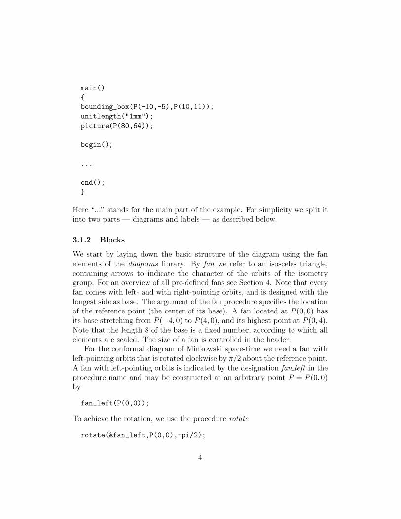
main()
{
bounding_box(P(-10,-5),P(10,11));
unitlength("1mm");
picture(P(80,64));
begin();
...
end();
}
Here “...” stands for the main part of the example. For simplicity we split itinto two parts — diagrams and labels — as described below.
3.1.2 Blocks
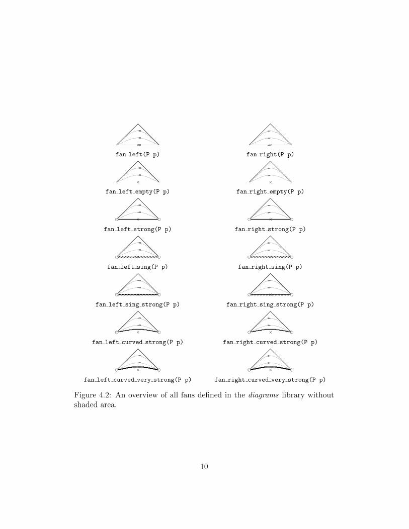
We start by laying down the basic structure of the diagram using the fanelements of the diagrams library. By fan we refer to an isosceles triangle,containing arrows to indicate the character of the orbits of the isometrygroup. For an overview of all pre-defined fans see Section 4. Note that everyfan comes with left- and with right-pointing orbits, and is designed with thelongest side as base. The argument of the fan procedure specifies the locationof the reference point (the center of its base). A fan located at P (0, 0) hasits base stretching from P (−4, 0) to P (4, 0), and its highest point at P (0, 4).Note that the length 8 of the base is a fixed number, according to which allelements are scaled. The size of a fan is controlled in the header.
For the conformal diagram of Minkowski space-time we need a fan withleft-pointing orbits that is rotated clockwise by π/2 about the reference point.A fan with left-pointing orbits is indicated by the designation fan left in theprocedure name and may be constructed at an arbitrary point P = P (0, 0)by
fan_left(P(0,0));
To achieve the rotation, we use the procedure rotate
rotate(&fan_left,P(0,0),-pi/2);
4
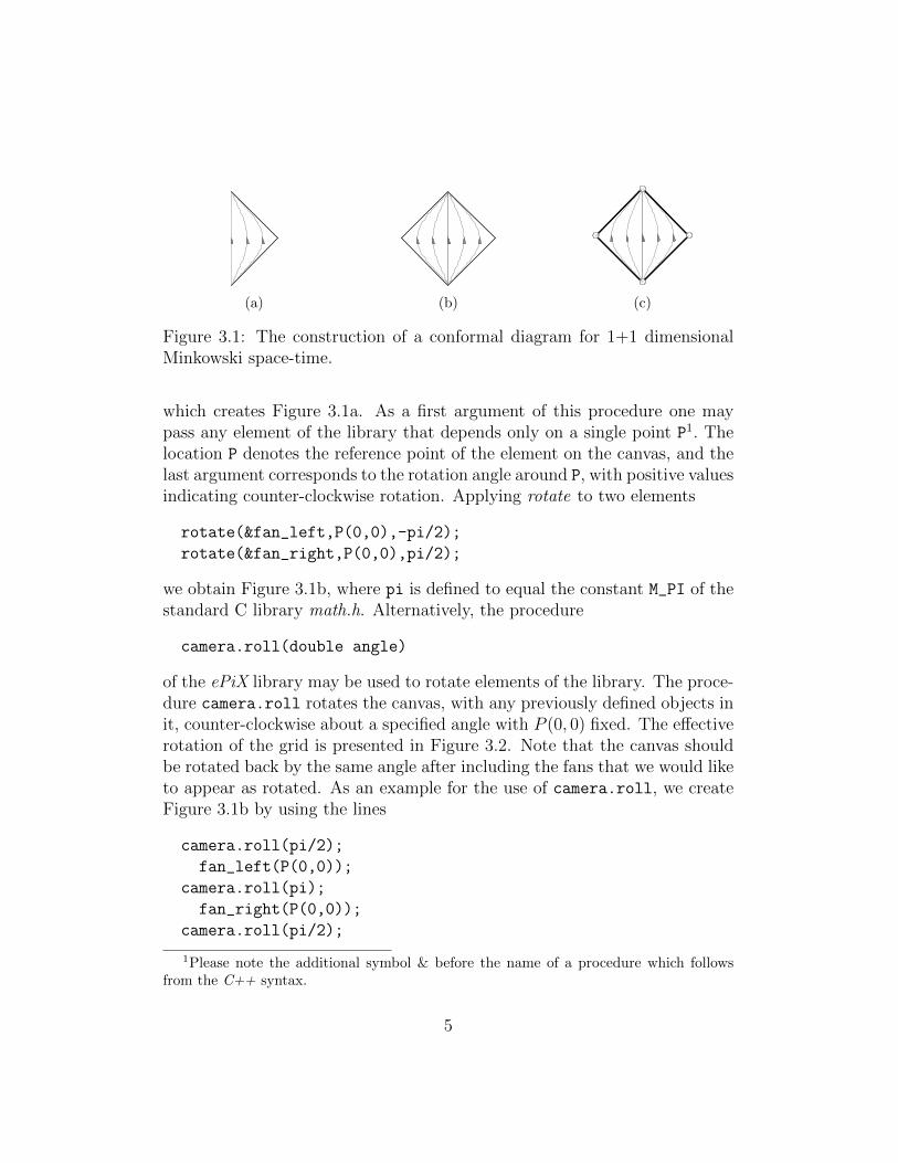
(a) (b) (c)
Figure 3.1: The construction of a conformal diagram for 1+1 dimensionalMinkowski space-time.
which creates Figure 3.1a. As a first argument of this procedure one maypass any element of the library that depends only on a single point P1. Thelocation P denotes the reference point of the element on the canvas, and thelast argument corresponds to the rotation angle around P, with positive valuesindicating counter-clockwise rotation. Applying rotate to two elements
rotate(&fan_left,P(0,0),-pi/2);
rotate(&fan_right,P(0,0),pi/2);
we obtain Figure 3.1b, where pi is defined to equal the constant M_PI of thestandard C library math.h. Alternatively, the procedure
camera.roll(double angle)
of the ePiX library may be used to rotate elements of the library. The proce-dure camera.roll rotates the canvas, with any previously defined objects init, counter-clockwise about a specified angle with P (0, 0) fixed. The effectiverotation of the grid is presented in Figure 3.2. Note that the canvas shouldbe rotated back by the same angle after including the fans that we would liketo appear as rotated. As an example for the use of camera.roll, we createFigure 3.1b by using the lines
camera.roll(pi/2);
fan_left(P(0,0));
camera.roll(pi);
fan_right(P(0,0));
camera.roll(pi/2);
1Please note the additional symbol & before the name of a procedure which followsfrom the C++ syntax.
5
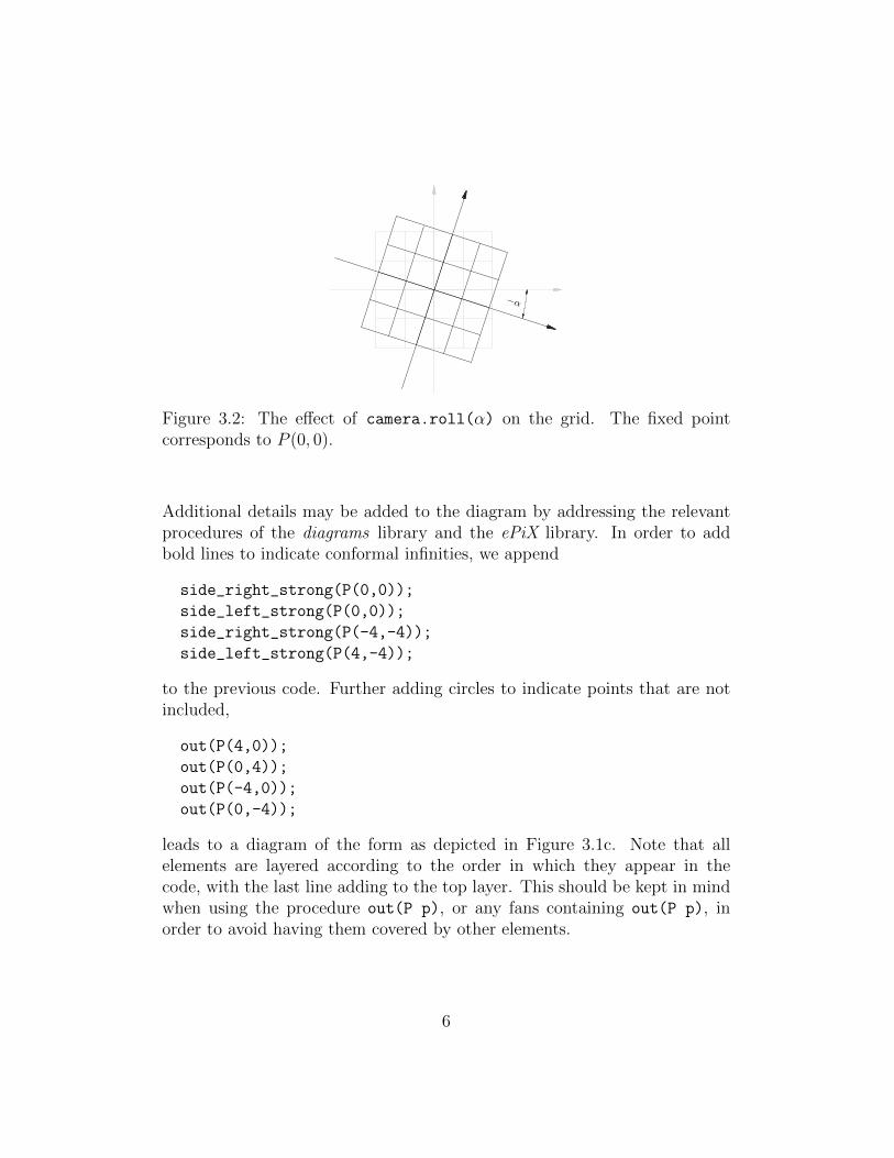
−α
Figure 3.2: The effect of camera.roll(α) on the grid. The fixed pointcorresponds to P (0, 0).
Additional details may be added to the diagram by addressing the relevantprocedures of the diagrams library and the ePiX library. In order to addbold lines to indicate conformal infinities, we append
side_right_strong(P(0,0));
side_left_strong(P(0,0));
side_right_strong(P(-4,-4));
side_left_strong(P(4,-4));
to the previous code. Further adding circles to indicate points that are notincluded,
out(P(4,0));
out(P(0,4));
out(P(-4,0));
out(P(0,-4));
leads to a diagram of the form as depicted in Figure 3.1c. Note that allelements are layered according to the order in which they appear in thecode, with the last line adding to the top layer. This should be kept in mindwhen using the procedure out(P p), or any fans containing out(P p), inorder to avoid having them covered by other elements.
6
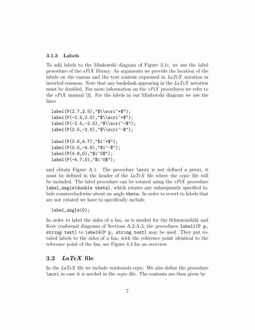
3.1.3 Labels
To add labels to the Minkowski diagram of Figure 3.1c, we use the labelprocedure of the ePiX library. As arguments we provide the location of thelabels on the canvas and the text content expressed in LaTeX notation ininverted commas. Note that any backslash appearing in the LaTeX notationmust be doubled. For more information on the ePiX procedures we refer tothe ePiX manual [3]. For the labels in our Minkowski diagram we use thelines
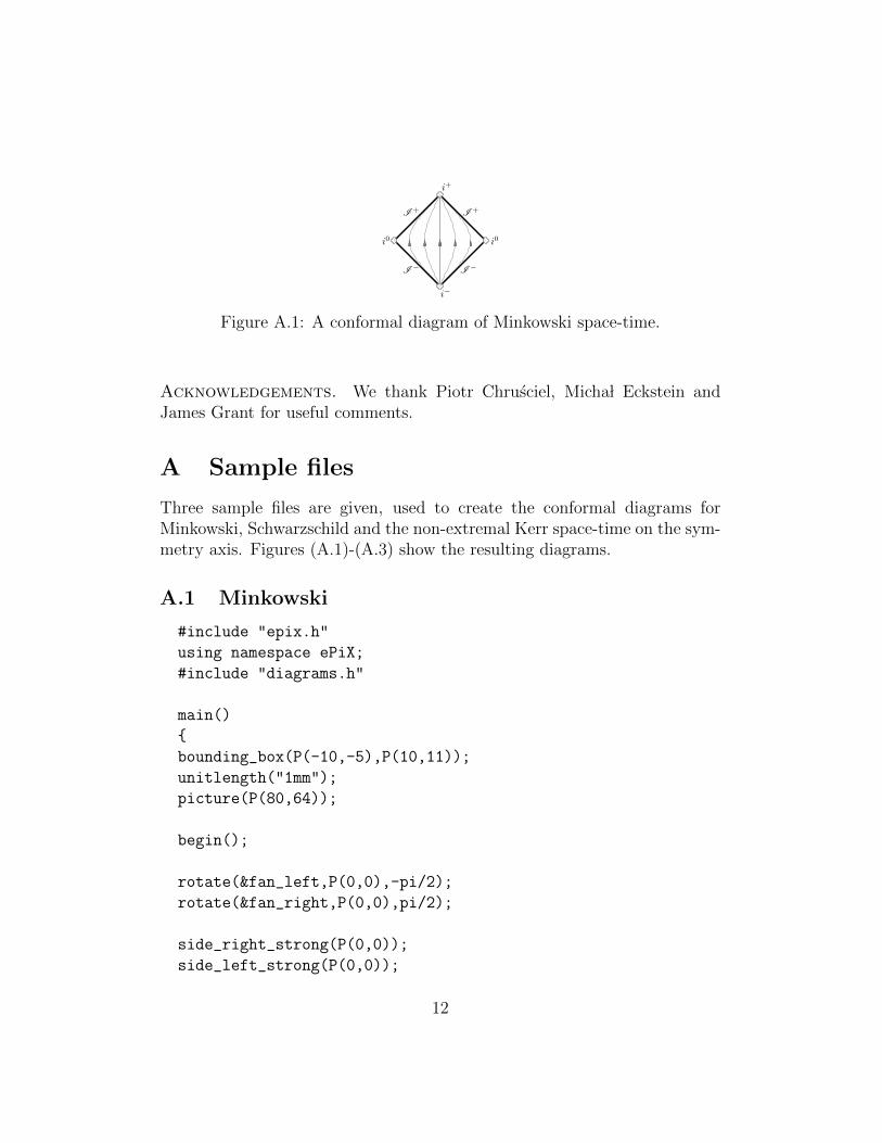
label(P(2.7,2.5),"$\\scri^+$");
label(P(-2.5,2.5),"$\\scri^+$");
label(P(-2.5,-2.5),"$\\scri^-$");
label(P(2.5,-2.5),"$\\scri^-$");
label(P(0.6,4.7),"$i^+$");
label(P(0.5,-4.6),"$i^-$");
label(P(4.8,0),"$i^0$");
label(P(-4.7,0),"$i^0$");
and obtain Figure A.1. The procedure \scri is not defined a priori, itmust be defined in the header of the LaTeX file where the eepic file willbe included. The label procedure can be rotated using the ePiX procedurelabel_angle(double theta), which rotates any subsequently specified la-bels counterclockwise about an angle theta. In order to revert to labels thatare not rotated we have to specifically include
label_angle(0);
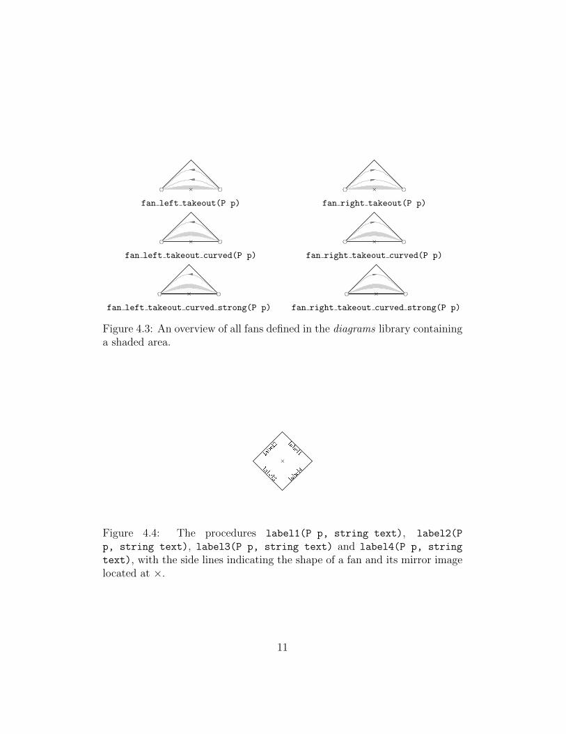
In order to label the sides of a fan, as is needed for the Schwarzschild andKerr conformal diagrams of Sections A.2-A.3, the procedures label1(P p,
string text) to label4(P p, string text) may be used. They put ro-tated labels to the sides of a fan, with the reference point identical to thereference point of the fan, see Figure 4.4 for an overview.
3.2 LaTeX file
In the LaTeX file we include minkowski.eepic. We also define the procedure\scri in case it is needed in the eepic file. The contents are then given by
7
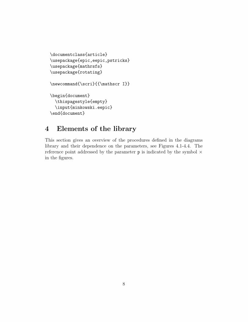
\documentclass{article}
\usepackage{epic,eepic,pstricks}
\usepackage{mathrsfs}
\usepackage{rotating}
\newcommand{\scri}{{\mathscr I}}
\begin{document}
\thispagestyle{empty}
\input{minkowski.eepic}
\end{document}
4 Elements of the library
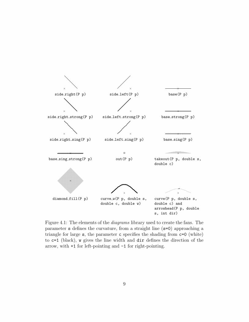
This section gives an overview of the procedures defined in the diagramslibrary and their dependence on the parameters, see Figures 4.1-4.4. Thereference point addressed by the parameter p is indicated by the symbol ×in the figures.
8
×
side right(P p)
×
side left(P p)
×
base(P p)
×
side right strong(P p)
×
side left strong(P p)
×
base strong(P p)
×
side right sing(P p)
×
side left sing(P p)
×
base sing(P p)
×
base sing strong(P p)
×
out(P p)
×
takeout(P p, double s,
double c)
×
diamond fill(P p)
×
curve w(P p, double s,
double c, double w)
×
curve(P p, double s,
double c) and
arrowhead(P p, double
s, int dir)
Figure 4.1: The elements of the diagrams library used to create the fans. Theparameter s defines the curvature, from a straight line (s=0) approaching atriangle for large s, the parameter c specifies the shading from c=0 (white)to c=1 (black), w gives the line width and dir defines the direction of thearrow, with +1 for left-pointing and -1 for right-pointing.
9
×
fan left(P p)
×
fan right(P p)
×
fan left empty(P p)
×
fan right empty(P p)
×
fan left strong(P p)
×
fan right strong(P p)
×
fan left sing(P p)
×
fan right sing(P p)
×
fan left sing strong(P p)
×
fan right sing strong(P p)
×
fan left curved strong(P p)
×
fan right curved strong(P p)
×
fan left curved very strong(P p)
×
fan right curved very strong(P p)
Figure 4.2: An overview of all fans defined in the diagrams library withoutshaded area.
10
×
fan left takeout(P p)
×
fan right takeout(P p)
×
fan left takeout curved(P p)
×
fan right takeout curved(P p)
×
fan left takeout curved strong(P p)
×
fan right takeout curved strong(P p)
Figure 4.3: An overview of all fans defined in the diagrams library containinga shaded area.
label1label2label3 label4×
Figure 4.4: The procedures label1(P p, string text), label2(P
p, string text), label3(P p, string text) and label4(P p, string
text), with the side lines indicating the shape of a fan and its mirror imagelocated at ×.
11
I +I +
I − I −
i+
i−
i0i0
Figure A.1: A conformal diagram of Minkowski space-time.
Acknowledgements. We thank Piotr Chrusciel, Micha l Eckstein andJames Grant for useful comments.
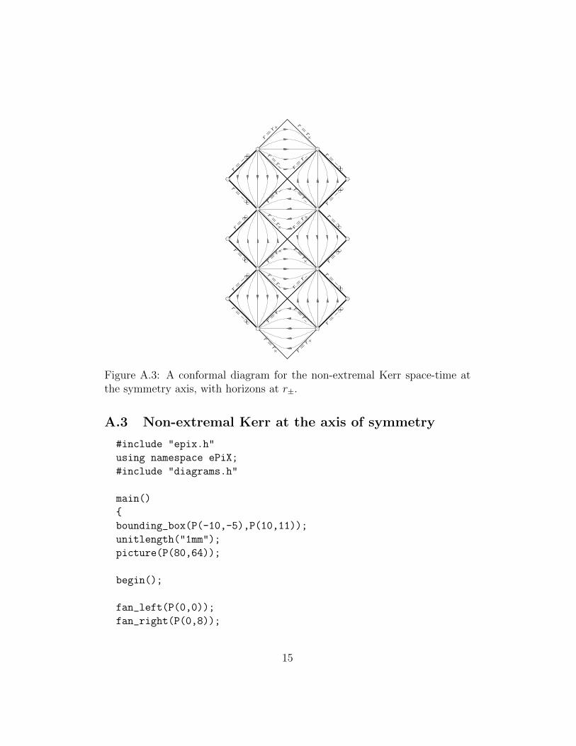
A Sample files
Three sample files are given, used to create the conformal diagrams forMinkowski, Schwarzschild and the non-extremal Kerr space-time on the sym-metry axis. Figures (A.1)-(A.3) show the resulting diagrams.
A.1 Minkowski
#include "epix.h"
using namespace ePiX;
#include "diagrams.h"
main()
{
bounding_box(P(-10,-5),P(10,11));
unitlength("1mm");
picture(P(80,64));
begin();
rotate(&fan_left,P(0,0),-pi/2);
rotate(&fan_right,P(0,0),pi/2);
side_right_strong(P(0,0));
side_left_strong(P(0,0));
12
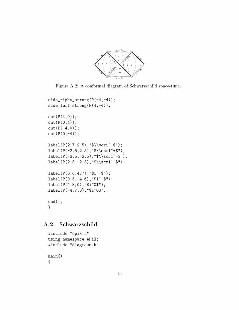
r = 0
r = 0
r=2m
r=2m
r=2m
r=2m
r=∞
r=∞
r=∞
r=∞
Figure A.2: A conformal diagram of Schwarzschild space-time.
side_right_strong(P(-4,-4));
side_left_strong(P(4,-4));
out(P(4,0));
out(P(0,4));
out(P(-4,0));
out(P(0,-4));
label(P(2.7,2.5),"$\\scri^+$");
label(P(-2.5,2.5),"$\\scri^+$");
label(P(-2.5,-2.5),"$\\scri^-$");
label(P(2.5,-2.5),"$\\scri^-$");
label(P(0.6,4.7),"$i^+$");
label(P(0.5,-4.6),"$i^-$");
label(P(4.8,0),"$i^0$");
label(P(-4.7,0),"$i^0$");
end();
}
A.2 Schwarzschild
#include "epix.h"
using namespace ePiX;
#include "diagrams.h"
main()
{
13
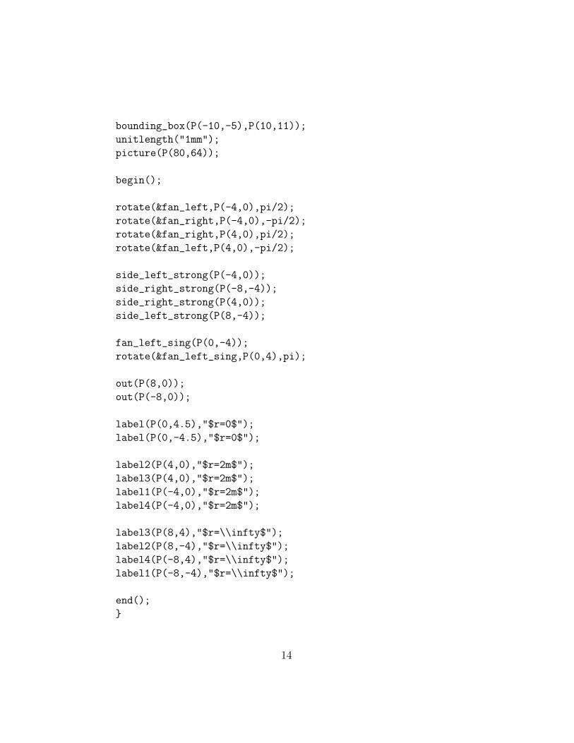
bounding_box(P(-10,-5),P(10,11));
unitlength("1mm");
picture(P(80,64));
begin();
rotate(&fan_left,P(-4,0),pi/2);
rotate(&fan_right,P(-4,0),-pi/2);
rotate(&fan_right,P(4,0),pi/2);
rotate(&fan_left,P(4,0),-pi/2);
side_left_strong(P(-4,0));
side_right_strong(P(-8,-4));
side_right_strong(P(4,0));
side_left_strong(P(8,-4));
fan_left_sing(P(0,-4));
rotate(&fan_left_sing,P(0,4),pi);
out(P(8,0));
out(P(-8,0));
label(P(0,4.5),"$r=0$");
label(P(0,-4.5),"$r=0$");
label2(P(4,0),"$r=2m$");
label3(P(4,0),"$r=2m$");
label1(P(-4,0),"$r=2m$");
label4(P(-4,0),"$r=2m$");
label3(P(8,4),"$r=\\infty$");
label2(P(8,-4),"$r=\\infty$");
label4(P(-8,4),"$r=\\infty$");
label1(P(-8,-4),"$r=\\infty$");
end();
}
14
r=r−r
=r−
r=r+ r
=r+
r=r− r
=r−
r=r+r
=r+
r=r− r
=r−
r=r−r
=r−
r=r+
r=r+
r=r+ r
=r+
r=−∞
r= −∞
r=∞
r=∞
r=−∞
r= −∞
r= −∞
r=−∞
r=∞
r=∞
r= −∞
r=−∞
Figure A.3: A conformal diagram for the non-extremal Kerr space-time atthe symmetry axis, with horizons at r±.
A.3 Non-extremal Kerr at the axis of symmetry
#include "epix.h"
using namespace ePiX;
#include "diagrams.h"
main()
{
bounding_box(P(-10,-5),P(10,11));
unitlength("1mm");
picture(P(80,64));
begin();
fan_left(P(0,0));
fan_right(P(0,8));
15
fan_left(P(0,-16));
fan_right(P(0,-8));
rotate(&fan_right,P(0,0),pi);
rotate(&fan_left,P(0,8),pi);
rotate(&fan_right,P(0,-16),pi);
rotate(&fan_left,P(0,-8),pi);
rotate(&fan_left,P(4,4),-pi/2);
rotate(&fan_right,P(4,-4),-pi/2);
rotate(&fan_left,P(4,-12),-pi/2);
rotate(&fan_left,P(-4,4),pi/2);
rotate(&fan_right,P(-4,-4),pi/2);
rotate(&fan_left,P(-4,-12),pi/2);
rotate(&fan_right,P(4,4),pi/2);
rotate(&fan_left,P(4,-4),pi/2);
rotate(&fan_right,P(4,-12),pi/2);
rotate(&fan_right,P(-4,4),-pi/2);
rotate(&fan_left,P(-4,-4),-pi/2);
rotate(&fan_right,P(-4,-12),-pi/2);
side_left_strong(P(8,0));
side_right_strong(P(-8,0));
side_left_strong(P(8,-8));
side_right_strong(P(-8,-8));
side_left_strong(P(8,-16));
side_right_strong(P(-8,-16));
side_left_strong(P(-4,4));
side_right_strong(P(4,4));
side_left_strong(P(-4,-4));
side_right_strong(P(4,-4));
16
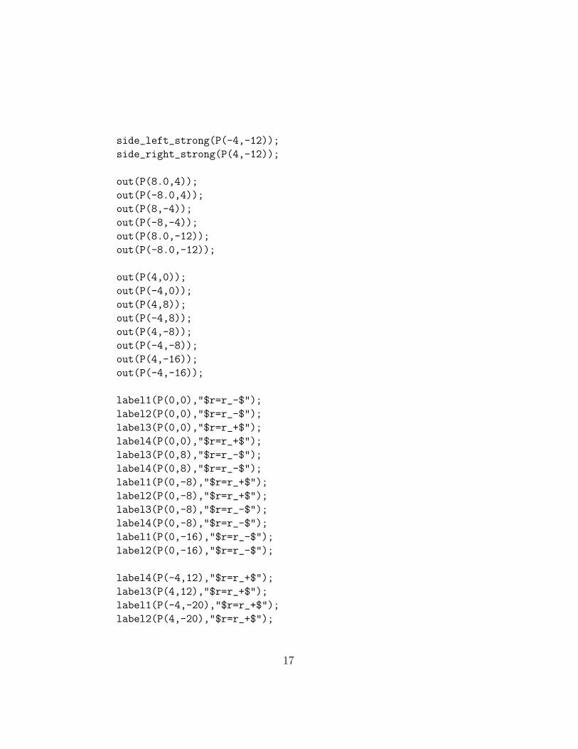
side_left_strong(P(-4,-12));
side_right_strong(P(4,-12));
out(P(8.0,4));
out(P(-8.0,4));
out(P(8,-4));
out(P(-8,-4));
out(P(8.0,-12));
out(P(-8.0,-12));
out(P(4,0));
out(P(-4,0));
out(P(4,8));
out(P(-4,8));
out(P(4,-8));
out(P(-4,-8));
out(P(4,-16));
out(P(-4,-16));
label1(P(0,0),"$r=r_-$");
label2(P(0,0),"$r=r_-$");
label3(P(0,0),"$r=r_+$");
label4(P(0,0),"$r=r_+$");
label3(P(0,8),"$r=r_-$");
label4(P(0,8),"$r=r_-$");
label1(P(0,-8),"$r=r_+$");
label2(P(0,-8),"$r=r_+$");
label3(P(0,-8),"$r=r_-$");
label4(P(0,-8),"$r=r_-$");
label1(P(0,-16),"$r=r_-$");
label2(P(0,-16),"$r=r_-$");
label4(P(-4,12),"$r=r_+$");
label3(P(4,12),"$r=r_+$");
label1(P(-4,-20),"$r=r_+$");
label2(P(4,-20),"$r=r_+$");
17
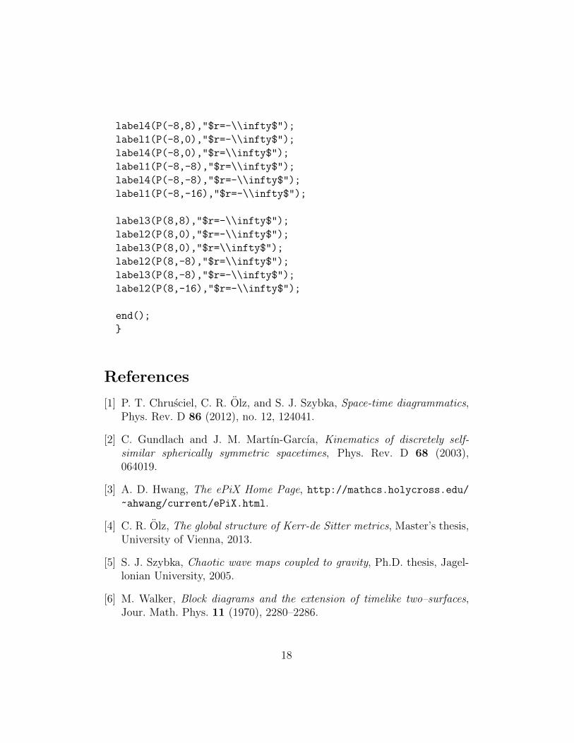
label4(P(-8,8),"$r=-\\infty$");
label1(P(-8,0),"$r=-\\infty$");
label4(P(-8,0),"$r=\\infty$");
label1(P(-8,-8),"$r=\\infty$");
label4(P(-8,-8),"$r=-\\infty$");
label1(P(-8,-16),"$r=-\\infty$");
label3(P(8,8),"$r=-\\infty$");
label2(P(8,0),"$r=-\\infty$");
label3(P(8,0),"$r=\\infty$");
label2(P(8,-8),"$r=\\infty$");
label3(P(8,-8),"$r=-\\infty$");
label2(P(8,-16),"$r=-\\infty$");
end();
}
References
[1] P. T. Chrusciel, C. R. Olz, and S. J. Szybka, Space-time diagrammatics,Phys. Rev. D 86 (2012), no. 12, 124041.
[2] C. Gundlach and J. M. Martın-Garcıa, Kinematics of discretely self-similar spherically symmetric spacetimes, Phys. Rev. D 68 (2003),064019.
[3] A. D. Hwang, The ePiX Home Page, http://mathcs.holycross.edu/
~ahwang/current/ePiX.html.
[4] C. R. Olz, The global structure of Kerr-de Sitter metrics, Master’s thesis,University of Vienna, 2013.
[5] S. J. Szybka, Chaotic wave maps coupled to gravity, Ph.D. thesis, Jagel-lonian University, 2005.
[6] M. Walker, Block diagrams and the extension of timelike two–surfaces,Jour. Math. Phys. 11 (1970), 2280–2286.
18