CONFORMAL MAPPING FOR THE EFFICIENT MFS … · conformal mapping for the efficient mfs solution of dirichlet boundary value problems ... in the case where

CONFORMAL MAPPING FOR THE EFFICIENT MFS SOLUTIONOF DIRICHLET BOUNDARY VALUE PROBLEMS∗

ANDREAS KARAGEORGHIS† AND YIORGOS–SOKRATIS SMYRLIS†

ABSTRACT. In this work, we use conformal mapping to transform harmonic Dirichlet problems that aredefined in simply–connected domains into harmonic Dirichlet problems that are defined in the unit disk.We then solve the resulting harmonic Dirichlet problems efficiently using the Method of Fundamental So-lutions (MFS) in conjunction with Fast Fourier Transforms (FFTs). This technique is extended to harmonicDirichlet problems in doubly–connected domains which are now mapped onto annular domains. Thesolution of the resulting harmonic Dirichlet problems can be carried out equally efficiently using the MFSwith FFTs. Several numerical examples are presented.

1. INTRODUCTION

In Trefftz methods [3, 11], the solution of a boundary value problem is approximated by a linear com-bination of special solutions of the governing equation of the problem in question. One such methodis the Method of Fundamental Solutions (MFS) in which the solution is approximated by a linearcombination of fundamental solutions of the operator of the governing equation, with singularities(sources) located outside the domain of the problem. The MFS has become increasingly popular inrecent years primarily due to the simplicity of its implementation. One of the fundamental questionsin the application of the MFS is the positioning of the sources. One way of dealing with this problemis to let the coordinates of the sources be free, and determine their locations by solving a non–linearleast–squares problem [5, 15]. However, this approach could be costly and has some drawbacks suchas the possibility of the existence of several minima in the non-linear least-squares minimization pro-cess. Alternatively, one may use the version of the MFS where the sources are preassigned (fixed) [6]on a pseudo-boundary surrounding, and usually similar in shape to, the boundary of the problem inquestion ([7]). The solution of Dirichlet harmonic problems in disks, when using the latter approach,has been the subject of several studies [9, 10, 20, 21, 22]. In these, convergence analyses and error esti-mates are presented, and efficient FFT-based methods are proposed. Similar results for Dirichlet har-monic problems in annular domains may be found in [27]. Both the theoretical and implementationalaspects of the MFS is these cases are well understood. Further, the conditioning of the coefficientmatrices arising in the MFS discretization is known to be poor. This ill–conditioning is exacerbatedwhen the domain of the problem under consideration is non–smooth, when the number of degrees offreedom becomes large, and when the distance of the pseudo–boundary from the boundary is large.These implementational difficulties may be alleviated in the case of domains with rotational symme-try. (See [20, Section 4.7].) In the general case of domains without rotational symmetry, the challengebecomes the determination of the distance of the pseudo-boundary from the boundary. One way ofovercoming this difficulty, proposed in [25], is to solve the boundary value problem with the MFS fora range of values of the distance of the pseudo–boundary from the boundary and for each distance

∗Technical Report TR–27–2007, Department of Mathematics and Statistics, University of Cyprus, October 2007.†This work was supported by University of Cyprus grant #8037-3/312-21005.‡Typeface Palatino, Mathpazo– System LATEX2ε.Date: October 29, 2007.2000 Mathematics Subject Classification. Primary 30C20, 35E05, 65N35; Secondary 30C30, 65N38.Key words and phrases. Method of fundamental solutions, Laplace equation, conformal mapping, circulant matrices.

1

2 A. KARAGEORGHIS AND Y.-S. SMYRLIS

find the maximum error in the satisfaction of the boundary conditions on a fixed set of boundarypoints (different from the MFS collocation points). The optimal value of this distance is the one forwhich the maximum error is minimal. This approach, however, requires the solution of a sequenceof problems and could be potentially expensive. In view of the fact that Dirichlet boundary valueproblems on disks and annuli may be solved efficiently, in this work we shall transform a given prob-lem in a simply–connected (resp. doubly–connected) domain into a problem in the unit disk (resp.an annulus) using conformal mappings and then to solve the transformed problem efficiently. In thisapproach, it is interesting to observe that when the conformal mapping opens up an angle, then a sin-gularity is introduced in the image point of the transformed domain. On the other hand, singularitiesdue, for example, to re–entrant corners can be removed by conformal transformations onto the disk.

The purpose of this paper is to show, apparently for the first time, how conformal mappings canbe used to transform harmonic Dirichlet problems in simply– and doubly–connected domains ontoproblems in the unit disk and appropriate annuli, respectively, where they can be solved efficientlyusing FFT–based matrix decomposition algorithms. Also, in this work we illustrate some of the po-tential difficulties associated with this technique, such as the introduction of boundary singularitiesin the transformed problems.

We consider the solution of Laplace’s equation in the complex z = x + iy−plane,

∆u = 0 in Ω, (1.1a)

subject to the Dirichlet boundary condition

u = f (x, y) on ∂Ω, (1.1b)

where the domain Ω is simply–connected. The idea is to use the conformal mapping F to transformproblem (1.1) into the boundary value problem in the complex w = ξ + iη−plane,

∆u = 0 in Ω,u = f (ξ, η) on ∂Ω,

(1.2)

where Ω is now the unit disk. If ξ + iη = x(ξ, η) + iy(ξ, η) is the image of x + iy under F , thenu(ξ, η) = u(x, y), and in particular, f (ξ, η) = f (x, y). Boundary value problem (1.2) can be solvedefficiently with the MFS using the techniques developed in [21, 22, 27].

The paper is organized as follows. In Section 2, we present several examples of problems in simply–connected domains which are mapped onto problems in the unit disk. In Section 3, we describe theefficient implementation of the MFS for the solution of harmonic Dirichlet problems in the unit disk.Numerical results for a number of examples are presented in Section 4. In Section 5, the techniquespresented in sections 2–3 are extended to the case of doubly–connected domains. Finally, in Section6, we provide some concluding remarks.

2. CONFORMAL MAPPINGS

The existence of conformal mappings for simply-connected domains is guaranteed from the Riemannmapping theorem (see e.g.,[29]) which states that If Ω is a simply–connected domain, other that C, andif z0 ∈ Ω, then there exists a unique conformal map F of Ω onto the unit disk so that F (z0) = 0 andF ′(z0) > 0. This mapping may be continuously extended from the boundary of Ω to the unit circle,if the former is a Jordan curve. (Caratheodory–Osgood Theorem [18].)

CONFORMAL MAPPING MFS ALGORITHMS 3

2.1. Exterior of an ellipse. We consider (1.1) in the complex plane when Ω is the exterior of an ellipse.More specifically, Ω is the exterior of the ellipse with major semi-axis a = cosh α and minor semi-axisb = sinh α in the complex z−plane. We know that the transformation [23]

z =12

(w e−α + w−1 eα

), (2.1)

maps the interior of the unit disk to the domain Ω of problem (1.1). The inverse of transformation(2.1) is given by

w = eα(

z−√

z2 − 1)

, (2.2)

and maps the domain Ω (z−plane) onto the interior of the unit disk (w−plane). Therefore, via trans-formation (2.2) the boundary value problem (1.1) in the z−plane with Ω the exterior of an ellipse ismapped onto problem (1.2) in the unit disk. The correspondence between the two domains is shownin Figure 1.

C A

B

D

z−plane

C′ A′

B′

D′

w−plane

FIGURE 1. Conformal mappings from exterior of ellipse to disk

2.2. Interior of an ellipse. We next consider problem (1.1) in the complex plane when Ω is the interiorof an elliptical domain, namely the interior of the ellipse with major semi-axis a > 1 and minor semi-axis b = 1 in the z−complex plane. The transformation ([16], page 296, see also [17])

w =√

k sn(

2K(k)π

sin−1( z√

a2 − 1

), k

), (2.3)

maps the interior of the ellipse Ω of problem (1.1) onto the interior of the unit disk. In the above,sn is the Jacobian elliptic sine and K(k) denotes the complete elliptic integral of the first kind withmodulus k. The inverse of transformation (2.3) is given by

z =√

a2 − 1 sin

π

2K(k)

∫ w√k

0

dt√(1− t2)(1− k2t2)

,

and maps the unit disk (w−plane) onto Ω (z−plane). Thus, via transformation (2.3) the boundaryvalue problem (1.1) in the interior of the ellipse in the z−plane is mapped onto problem 1.2 in theunit disk. The correspondence between the two domains is shown in Figure 2. It should be noted thatthe modulud k satisfies

K(k′)K(k)

=2π

sinh−1(

2aa2 − 1

), (2.4)

where k′ =√

1− k2.


C A

D

B

z−plane

C′ A′

B′

D′

w−plane

FIGURE 2. Conformal mappings from interior of ellipse to disk.

2.3. Cardioid. We next consider problem (1.1) in the complex plane when Ω is the interior of a car-dioid, defined parametrically in polar coordinates by r = 2a2(1 + cos θ) in the complex z−plane. Thecardioid is mapped onto the interior of a disk of radius a with centre v = a in the v−plane, via thetransformation [23]

v = z1/2. (2.5)

The inverse mapping is given by

z = v2.

This disk is subsequently mapped onto the unit disk via

w =1a

(v− a), (2.6)

while the inverse mapping is given by

v = aw + a.

Thus, via transformation (2.5) boundary value problem (1.1) in the interior of the cardioid in thez−plane is mapped onto a problem in a disk with centre v = a and radius a in the v−plane. Subse-quently, this problem is mapped onto problem 1.2 in the unit disk in the w−plane via transformation(2.6). The correspondence between the three domains is shown in Figure 3.

z−plane v−plane w−plane

FIGURE 3. Conformal mappings from interior of cardioid to disk.


z −K + iK′ −K 0 K K + iK′ iK′

v −k−1 −1 0 1 k−1 ∞

w e2i tan−1 k i −1 −i e−2i tan−1 k 1TABLE 1. Correspondence of points in z−, v− and w−planes for rectangle.

z A B Cv 0 1 ∞w −1 −i 1

TABLE 2. Correspondence of points in z−, v− and w−planes for triangle.

2.4. Rectangular domain. We now consider problem (1.1) in the complex z−plane, in the case whereΩ is a rectangle with corners −K, K, K + iK′,−K + iK′, where K and K′ are the complete ellipticintegrals of the first kind with moduli k < 1 and k′ =

√1− k2, respectively. The problem is first

mapped onto the upper half plane of the v−plane via the transformation given by the Jacobian ellipticfunction [16]

v = sn z.

The inverse mapping is given by the incomplete elliptic integral of the first kind [16]

z =∫ v

0

dv√(1− v2) (1− k2v2)

= sn−1(v, k). (2.7)

In (2.7), the modulus k depends on the ratio K′/K. For 0.3 ≤ K′/K ≤ 3, the corresponding valuesof k may be found in [1], Table 17.3. The correspondence of the various points of the boundary ∂Ω ofthe rectangle and points on the real line are given in Table 1 [16]. From the upper half–plane in thev−plane onto the unit disk in the w−plane, we use the transformation

w =v− iv + i

(2.8)

which has the inverse transformation

v = i1 + w1− w

. (2.9)

The correspondence between the key points on the upper half-plane and the boundary of the unitdisk are given in Table 1. The transformations are presented in Figure 4.

2.5. Triangular domain. Finally, we consider problem (1.1) in the complex z−plane when Ω is thetriangle ABC with A = (0, 0) and B lying on the positive real axis. Here, we adopt the notation forthe angles CAB = α and ABC = β. The problem is first mapped onto the upper half plane andsubsequently onto the unit disk via transformations (2.8)-(2.9). The upper half plane is mapped ontothe interior of the triangle ABC via the Schwarz–Christoffel transformation [13, 16]

z =∫ v

0t

απ−1 (1− t)

βπ−1 dt. (2.10)

Clearly the point A is mapped onto the origin of the upper half plane, B onto 1 and C onto infinity.The correspondence of the vertices of the triangle ABC to the various points on the real line and thedisk are presented in Table 2, while the transformations are presented in Figure 5.


−K O K

K+iK′−K+iK′ z−plane

−k−1 −1 O 1 k−1• • • • •

v−plane

−1 1

−i

i eiθ

e−iθ

• •

•

• •

•

w−plane

FIGURE 4. Conformal mappings from rectangle to disk.

3. METHOD OF FUNDAMENTAL SOLUTIONS

In the MFS, the solution u of problem (1.2) is approximated by the harmonic function [15, 19]

uN(c, Q; P) =N

∑`=1

c`K(P, Qα` ), P∈ Ω,

where c = (c1, c2, . . . , cN)T and Q is a 2N−vector containing the coordinates of the singularities

(sources) Qα` , ` = 1, . . . , N, which lie outside Ω. The function K(P, Q) is a fundamental solution of

the Laplacian given by

K(P, Q) = − 12π

log |P−Q|, (3.1)

with |P−Q| denoting the distance between the points P and Q. The singularities Qα` are fixed on the

boundary ∂Ω′ of a disk Ω′ concentric to the unit disk Ω and defined by Ω′ = x ∈ R2 : |x| < R,where R > 1. A set of collocation points PkN

k=1 is placed on ∂Ω. If Pk = (xPk , yPk ), then we take

xPk = cos2(k− 1)π

N, yPk = sin

2(k− 1)π

N, k = 1, . . . , N.

If Qαj =

(xQα

j, yQα

j

), then

xQα`

= R cos2(`− 1 + α)π

N, yQα

`= R sin

2(`− 1 + α)π

N, ` = 1, . . . , N, (3.2)

where the positions of the sources differ by an angle2πα

Nfrom the positions of the boundary points

and 0 ≤ α < 1. In the case α 6= 0, we thus have a rotation of the singularities with respect to theboundary points. This rotation is performed in order to obtain improved results when R− 1 ¿ 1.


Aα

Bβ

C

z−plane

A′ B′ (1) C′ C′

v−plane

• •

−1 1

−i

i

• •

•

w−plane

FIGURE 5. Conformal mappings from triangle to disk.

The coefficients c are determined so that the boundary condition is satisfied at the boundary pointsPkN

k=1:uN(c, Q; Pk) = f (Pk), k = 1, . . . , N.

With obvious notation for f , this yields a linear system of the form

Gαc = f , (3.3)

for the coefficients c, where the elements of the matrix Gα are given by

Gαk,` = − 1

2πlog |Pk −Qα

` |, k, ` = 1, . . . , N.

Clearly, Gα is a circulant matrix and the system (3.3) can be solved efficiently using the matrix decom-position algorithm of [21, 22]. If U∗ = 1√

N(e2πi(k−1)(`−1)/N)N

k,`=1, we premultiply system (3.3) by U

to obtain UGαU∗Uc = U f or DUc = U f or Dc = f , where c = Uc and f = U f and the matrixD is diagonal [4], with entries

dj

Nj=1. The solution is thus clearly, ci = fi/di, i = 1, . . . , N. Having

obtained c, we can find c from c = U∗ c. We thus have the following matrix decomposition algorithm[21, 22]:

Algorithm.

Step 1. Compute f = U f.

Step 2. Construct the diagonal matrix D.

Step 3. Evaluate c.

Step 4. Compute c = U∗ c.


Cost. This algorithm requires O(N log N) operations.

An efficient MATLAB code implementation of the method described in this section is presented inAppendix I. In it, the maximum error on the boundary is calculated in the case f (x, y) = e4x cos 4y.

4. NUMERICAL RESULTS

In all numerical examples, the maximum relative error on 25 uniformly distributed points (which arenot collocation points) on the boundary of the unit circle was calculated for various values of N.

Example 1: Exterior of an ellipse. We first consider problem (1.1) in which Ω is the domain exteriorto the ellipses defined by α = 0.1, 0.5. The boundary condition is taken to be f (z) = z−1 and the plotsof the maximum relative error versus R are presented in Figure 8. The error in the case α = 0.1 ismuch larger that in the case α = 0.5, as the aspect ratio in the former case is much larger. In particular,in the case α = 0.1 the ratio of the length of the major axis with respect to the length of the minor axisis 10.0333 whereas in the case α = 0.5 it is 2.1640. Also, the conformal mapping given by (2.2) has asingularity at z = ±1 and in the case α = 0.1, the boundary is much closer to the singular pointsthan in the case α = 0.5.

Example 2: Interior of an ellipse. We consider the case in which the ellipse is defined by semi-minoraxis b = 1 and major axis a > 1. In (2.4) we chose k = 3/4, 1/2 and 1/3 which corresponds toa = 1.8285, 1.5249 and 1.3785, respectively. The boundary condition is taken to be f (z) = z2 and theplots of the maximum relative error versus R are presented in Figure 9. As in the case of the exteriorellipse, we observe that the error is smaller for smaller values of the aspect ratio of the ellipse (a/b).

Also, the mapping function has dominant simple poles at z = ± 2ai√a2 − 1

, and as a increases the

boundary approaches these poles resulting in poor convergence. (See [17].)

Example 3: Cardioid. We consider the case of a cardioid defined by a = 1. The boundary conditionwas taken to be f (z) = z5. The plot of the maximum relative error versus R is presented in Figure 10and from it we observe extremely rapid convergence of the method.

Example 4: Rectangular domain. We first consider the rectangle for which K′/K = 1. In this case,it follows that k = 1/

√2. We considered two cases, when the boundary conditions are f (z) = z2

and f (z) = sin z, respectively. The plots of the maximum relative error versus R are presented inFigure 11. From these it is observed in order to obtain high accuracy, large values of N are requiredand the high accuracy occurs only in a small range of values of R, relatively close to the boundary.This is typical of the behaviour of the MFS for problems with boundary singularities. In Figure 12 wepresent f (v) on the boundary of the disk, for f (z) = z2 and f (z) = sin z. From these it is clear thatboundary singularities are introduced at the points corresponding to the corners of the rectangle.

We also considered the square i.e., K′/K = 2. From [1, Table 17.3] it follows that, in this case, k2 =0.0294372515. Again we considered the two cases when the boundary condition is f (z) = z2 andf (z) = sin z, respectively. In Figure 13, we present the plots of the maximum relative error versusR in the two cases. As expected the errors are considerably smaller than the errors obtained forthe rectangle defined by K′/K = 1. In Figure 14, we present f (v) on the boundary of the disk, forf (z) = z2 and f (z) = sin z and as in the previous case, it is clear that singularities are introduced atthe points corresponding to the corners of the square.

When going from the rectangle to the unit disk the conformal transformation introduces singularitiesat the images of at the corners of the four right angles in the sense that the first derivatives of thesolution of the transformed problem becomes unbounded there. (See [14].)


Example 5: Triangular domain. We considered two cases, an equilateral triangle (α = β = π/3) anda right–angled triangle (α = π/3, β = π/2 ). The boundary condition is taken to be f (z) = sin zand the plots of the maximum relative error versus R are presented in Figure 15. As in the case ofthe rectangle, it is observed that high accuracy is only achieved for large values of N and the highaccuracy occurs only in a small range of values of R, relatively close to the boundary. In Figure 16, wepresent f (w) on the boundary of the disk, for the two triangles. As in the case of the rectangle, it isclear that singularities are introduced at the points corresponding to the corners of the rectangle, dueto the opening–up of the angles of the triangles.

5. DOUBLY CONNECTED DOMAINS

In this section we extend the the ideas of Section 2 to doubly connected domains. For the existenceof such conformal mappings we rely on the fact that any doubly connected domain can be mapped con-formally onto an annulus ([29]). It should be noted that the annulus onto which the doubly–connecteddomain is mapped onto is one with a specific ratio of its two radii. (This ratio is called the conformalmodulus of the domain.)

The solution of Laplace’s equation in annular domains subject to Dirichlet boundary conditions canbe solved very efficiently as will be explained in the sequel.

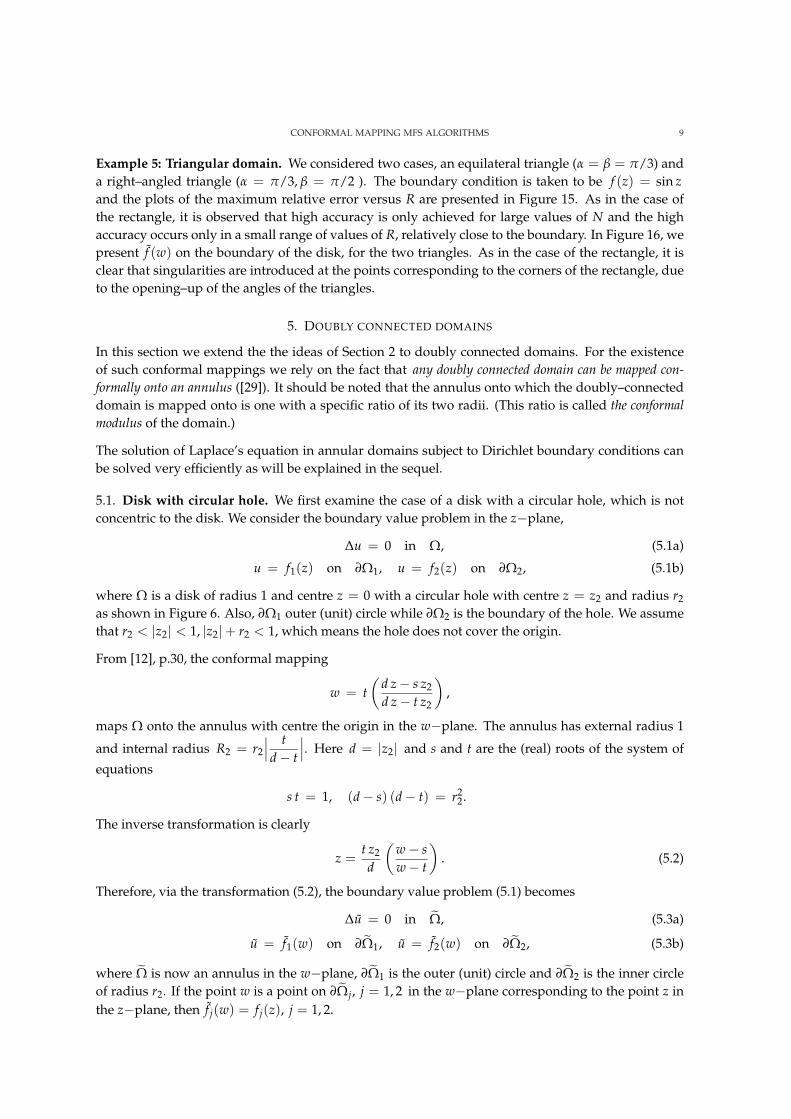
5.1. Disk with circular hole. We first examine the case of a disk with a circular hole, which is notconcentric to the disk. We consider the boundary value problem in the z−plane,

∆u = 0 in Ω, (5.1a)

u = f1(z) on ∂Ω1, u = f2(z) on ∂Ω2, (5.1b)

where Ω is a disk of radius 1 and centre z = 0 with a circular hole with centre z = z2 and radius r2

as shown in Figure 6. Also, ∂Ω1 outer (unit) circle while ∂Ω2 is the boundary of the hole. We assumethat r2 < |z2| < 1, |z2|+ r2 < 1, which means the hole does not cover the origin.

From [12], p.30, the conformal mapping

w = t(

d z− s z2

d z− t z2

),

maps Ω onto the annulus with centre the origin in the w−plane. The annulus has external radius 1

and internal radius R2 = r2

∣∣∣ td− t

∣∣∣. Here d = |z2| and s and t are the (real) roots of the system of

equations

s t = 1, (d− s) (d− t) = r22.

The inverse transformation is clearly

z =t z2

d

(w− sw− t

). (5.2)

Therefore, via the transformation (5.2), the boundary value problem (5.1) becomes

∆u = 0 in Ω, (5.3a)

u = f1(w) on ∂Ω1, u = f2(w) on ∂Ω2, (5.3b)

where Ω is now an annulus in the w−plane, ∂Ω1 is the outer (unit) circle and ∂Ω2 is the inner circleof radius r2. If the point w is a point on ∂Ωj, j = 1, 2 in the w−plane corresponding to the point z inthe z−plane, then f j(w) = f j(z), j = 1, 2.


z−plane

z2•

•

w−plane

FIGURE 6. Conformal mapping from a disk with non–concentric hole to an annulus.

5.2. Two concentric ellipses. We next consider the case of the region between two concentric ellipses:

L0 :x2

a20

+y2

b20

= 1 and L1 :x2

a21

+y2

b21

= 1,

that is, we consider boundary value problem (5.1) where Ω is an ellipse with boundary ∂Ω1 = L0

with a concentric elliptical hole with boundary ∂Ω0 = L1. In the case when the ellipses are confocal,that is, a2

0 − b20 = a2

1 − b21, the conformal mapping [24]

w =z +

√z2 − (a2

0 − b20)

a0 + b0, (5.4)

maps the domain Ω in the z−plane onto the annulus Ω in the w−plane. In this case, Ω has outer

radius one and inner radius R2 =a1 + b1

a0 + b0. The inverse transformation is given by

z =a0 − b0 + (a0 + b0)w2

2w. (5.5)

Thus, via transformation (5.4), boundary value problem (5.1) becomes (5.3) in the w−plane, as shownin Figure 7. As in the previous example, if the point w is a point on ∂Ωj, j = 1, 2 in the w−planecorresponding to the point z in the z−plane, then f j(w) = f j(z), j = 1, 2.

FIGURE 7. Conformal mapping from concentric ellipses to annulus.


5.3. Method of fundamental solutions for annular domains. In the case of the annulus, following[27], we approximate the solution u of problem (5.3) by

uN(c1, c2, Q1, Q2; P) =N

∑`=1

c1`K(P, Q1,α

` ) +N

∑`=1

c2`K(P, Q2,α

` ), P∈Ω,

where cj = (cj1 , cj2 , . . . , cjN )T , j = 1, 2 and Qj are 2N−vectors containing the coordinates of the

singularities (sources) Qj,α` , ` = 1, . . . , N, j = 1, 2, which lie outside Ω. The function K(P, Q) is a

fundamental solution of Laplace’s equation given by (3.1). The singularities Q1,α` are fixed on the

circle ∂Ω′1 concentric to the unit circle ∂Ω1 and defined by ∂Ω′ = x∈R2 : |x| = R, where R > 1.

Similarly, the singularities Q2,α` are fixed on the circle ∂Ω′

2 concentric to the circle ∂Ω2 and defined by∂Ω′ = x∈R2 : |x| = r, where r < R2.

A set of collocation points PjkN

k=1, j = 1, 2 is placed on ∂Ωj, j = 1, 2. If Pjk = (x

Pjk, y

Pjk), then we take

xP1k

= cos2(k− 1)π

N, yP1

k= sin

2(k− 1)π

N, k = 1, . . . , N.

and

xP2k

= R2 cos2(k− 1)π

N, yP2

k= R2 sin

2(k− 1)π

N, k = 1, . . . , N.

If Qj,α` =

(x

Qj,α`

, yQj,α

`

), j = 1, 2, then

xQ1,α`

= R cos2(`− 1 + α)π

N, yQ1,α

`= R sin

2(`− 1 + α)π

N, ` = 1, . . . , N,

and

xQ2,α`

= r cos2(`− 1 + α)π

N, yQ2,α

`= r sin

2(`− 1 + α)π

N, ` = 1, . . . , N,

where α is as in (3.2). The coefficients cj, j = 1, 2 are determined so that the boundary conditions aresatisfied at the boundary points PjkN

k=1, j = 1, 2:

uN(c1, c2, Q1, Q2; P1k ) = f1(P1k ) and uN(c1, c2, Q1, Q2; P2k ) = f2(P2k ), k = 1, . . . , N. (5.6)

With obvious notation for f 1 and f 2, this yields a linear system of the form(

Gα11 Gα

12Gα

21 Gα22

) (c1

c2

)=

(f 1f 2

), (5.7)

where the elements of the matrices Gαjm, j, m = 1, 2 are given by

Gαjmk,`

= − 12π

log |Pjk −Qαm`|, k = 1, . . . , N ` = 1, . . . , N, j, m = 1, 2, (5.8)

Clearly, each of the matrices Gαjm, j, m = 1, 2 is circulant and the system (5.7) can be solved efficiently

as is shown in [27]. If I2 is the identity matrix of order 2, we premultiply system (5.7) by I2 ⊗U toobtain

(U 00 U

) (Gα

11 Gα12

Gα21 Gα

22

) (U∗ 00 U∗

) (U 00 U

) (c1

c2

)=

(U 00 U

) (f 1f 2

),

or (D11 D12

D21 D22

) (c1

c2

)=

(f 1f 2

), (5.9)


where cj = Ucj, f j = U f j, j = 1, 2, and each of the matrices Djm, j, m = 1, 2 is diagonal withentries djmk

, k = 1, . . . N, j, m = 1, 2. System (5.9) is therefore equivalent to the N independent 2× 2systems (

d11k d12k

d21k d22k

) (c1k

c2k

)=

(f1k

f2k

), k = 1, . . . N,

from which we get

c1k =d22k f1k − d12k f2k

d11k d22k − d12k d22k

and c2k =d11k f2k − d21k f2k

d11k d22k − d12k d22k

, k = 1, . . . N.

The solution is thus clearly, ci = f i/di, i = 1, . . . , N. Having obtained cj, j = 1, 2, we can findc, j = 1, 2 from cj = U∗ cj, j = 1, 2. We thus have the following matrix decomposition algorithm [27]:

Algorithm

Step 1. Compute f j = U f j, j = 1, 2.

Step 2. Construct the diagonal matrices Djm, j, m = 1, 2.

Step 3. Evaluate cj, j = 1, 2.

Step 4. Compute cj = U∗ cj, j = 1, 2.

Cost. As in the case of the disk, this algorithm can be carried out at O(N log N) operations.

An efficient MATLAB code implementing the method described in this section is presented in Ap-pendix II. As in the case of the unit disk, the maximum error on the boundary, when the boundarycondition is f (x, y) = e4x cos 4y, is calculated.

5.4. Numerical results. In the following numerical examples, the maximum relative error was calcu-lated on 25 uniformly distributed points on each of the boundary circle of the annulus.

Example 6: Disk with circular hole. We considered the case of the unit disk with a hole with centrez2 = 0.3 + 0.3i and radius r2 = 0.3 which is mapped onto the annulus with external boundary theunit circle and internal boundary a circle with radius R2 = 0.37636943446018 and we took the internalpseudo–boundary to be fixed with radius r = 0.25. The boundary condition is f (z) = 1/(z− z2).We kept the internal pseudo–boundary fixed with radius r = R2/2. The plot of the maximum relativeerror versus R are presented in Figure 17 and from it we observe extremely rapid convergence of themethod.

Example 7: Two concentric ellipses. We considered the cases when a0 = 9, b0 = 7, a1 = 6, b1 = 2and a0 = 7, b0 = 5, a1 = 5, b1 = 1. In both cases, the annulus has inner radius R2 = 0.5. Theboundary condition was taken to be f (z) = 1/z. The plots of the maximum relative error versusR are presented in Figure 18. In the first case, the convergence is more rapid because of the smalleraspect ratio of the internal ellipse.

6. CONCLUDING REMARKS

In this paper, we applied conformal mappings to harmonic Dirichlet problems in various simply– anddoubly–connected domains yielding harmonic Dirichlet problems on the unit disk or an appropriateannulus. The solution of such problems using the MFS yields linear systems in which the coefficientmatrices are circulant and can therefore be solved very efficiently using FFTs. Further, this removespotential sources of ill–conditioning which are inherent in the application of the MFS to simply– anddoubly–connected domains. There is a potential difficulty when applying this technique to problemsin non-convex polygonal domains. In these cases, the conformal transformations mapping these do-mains onto the disk introduce boundary singularities at the points corresponding to the non-convex


vertices. The reason for this is that these points are singularities of the Schwarz–Christoffel transfor-mation mapping the polygon onto the upper half–plane. This means that, in such cases, more degreesof freedom are required for the accurate solution of the problem. Also, the range of the radii of thepseudo-boundaries for which accurate MFS solutions are obtained is shorter than in other problems.However, in view of the very efficient solution of the Dirichlet problem in the disk or an annulus, thismay still be viewed as an improvement. In the future we intend to apply the technique described inthe paper to more complex problems for which no analytical expressions for the conformal mappingexist, using numerical conformal mapping software such as BKMPACKJ [28], CONFPACK [8], SCPACK[26].

ACKNOWLEDGEMENTS

The authors are grateful to Professors Graeme Fairweather and Nick Papamichael for helpful discus-sions.

APPENDIX I

MATLAB code for the efficient solution of Dirichlet problem in the unit disk

function laplf(f,mp,iter,ds,alfa,m)

coe=-(1.0/(2.0*pi)); theta=2.0*pi/m; rp=1.0;

for ii=1:iter

rs=rp+ii*ds; (or alfa= (0.5*ii/(iter+1)))

ang=theta*(0:m-1); ca=cos(ang);sa=sin(ang);

ca1=cos(ang+theta*alfa);sa1=sin(ang+theta*alfa);

xp=rp*ca;yp=rp*sa;xs=rs*ca1;ys=rs*sa1; b=feval(f,xp,yp)’;

dx=xp(1)*ones(1,m)-xs; dy=yp(1)*ones(1,m)-ys;

aa=.5*coe*log(dx.*dx+dy.*dy); om=exp(2.0*pi*i/m); oc=conj(om);

d=ifft(aa’); ff=fft(b)/sqrt(m); c=ff./d;

ct=real(ifft(c)/sqrt(m));

the=2.0*pi/mp; ang=the*(0:mp-1);ca=cos(ang);sa=sin(ang);

xx=rp*ca;yy=rp*sa; exa=feval(f,xx,yy);

dx=xs’*ones(1,mp)-ones(m,1)*xx; dy=ys’*ones(1,mp)-ones(m,1)*yy;

rh=.5*coe*log(dx.*dx+dy.*dy);

err=rh’*ct-exa’; a1=max(abs(err));

rt(ii,1)=rs; (or rt(ii,1)=alfa;) rt(ii,2)=a1;

end

semilogy(rt(:,1),rt(:,2),’-’) (or plot(rt(:,1),rt(:,2),’-’))

function f=f1(x,y)

f=exp(4.*x).*cos(4.*y);


APPENDIX II

MATLAB code for the efficient solution of Dirichlet problem in an annulus

function lapannef(f,mp,iter,ds,alfa,m)

cf=-(1.0/(4.0*pi));theta=2.0*pi/m; rpe=1.0; rpi=0.5;

os=ones(1,m);op=ones(1,mp);ot=ones(m,1);

for ii=1:iter

rse=rpe+ii*ds;rsi=rpi/2;

ang=theta*(0:m-1); ca=cos(ang);sa=sin(ang);

ca1=cos(ang+theta*alfa);sa1=sin(ang+theta*alfa);

xpe=rpe*ca;ype=rpe*sa;xpi=rpi*ca;ypi=rpi*sa;

xse=rse*ca1;yse=rse*sa1;xsi=rsi*ca1;ysi=rsi*sa1;

be=feval(f,xpe,ype)’;bi=feval(f,xpi,ypi)’;

dxee=xpe(1)*os-xse;dyee=ype(1)*os-yse;aee=cf*log(dxee.*dxee+dyee.*dyee);

dxei=xpe(1)*os-xsi;dyei=ype(1)*os-ysi;aei=cf*log(dxei.*dxei+dyei.*dyei);

dxie=xpi(1)*os-xse;dyie=ypi(1)*os-yse;aie=cf*log(dxie.*dxie+dyie.*dyie);

dxii=xpi(1)*os-xsi;dyii=ypi(1)*os-ysi;aii=cf*log(dxii.*dxii+dyii.*dyii);

om=exp(2.0*pi*i/m);oc=conj(om);

dee=ifft(aee’);dei=ifft(aei’);die=ifft(aie’);dii=ifft(aii’);

ffe=fft(be)/sqrt(m);ffi=fft(bi)/sqrt(m);

ce=(dii.*ffe-dei.*ffi)./(dii.*dee-dei.*die);

ci=(-die.*ffe+dee.*ffi)./(dii.*dee-dei.*die);

cte=ifft(ce)/sqrt(m);cti=ifft(ci)/sqrt(m);

the=2.0*pi/mp;ang=the*(0:mp-1);ca=cos(ang);sa=sin(ang);

xxe=rpe*ca;yye=rpe*sa;exae=feval(f,xxe,yye);

xxi=rpi*ca;yyi=rpi*sa;exai=feval(f,xxi,yyi);

dxee=xse’*op-ot*xxe;dyee=yse’*op-ot*yye;

dxei=xsi’*op-ot*xxe;dyei=ysi’*op-ot*yye;

rhe=cf*log(dxee.*dxee+dyee.*dyee);rhi=cf*log(dxei.*dxei+dyei.*dyei);

erre=rhe’*cte+rhi’*cti-exae.’;

dxie=xse’*op-ot*xxi;dyie=yse’*op-ot*yyi;

dxii=xsi’*op-ot*xxi;dyii=ysi’*op-ot*yyi;

rhe=cf*log(dxie.*dxie+dyie.*dyie);rhi=cf*log(dxii.*dxii+dyii.*dyii);

erri=rhe’*cte+rhi’*cti-exai.’;

a1i=max(abs(erri));a1e=max(abs(erre));a1=max(a1i,a1e);

rt(ii,1)=rse; rt(ii,2)=a1;

end

semilogy(rt(:,1),rt(:,2),’-’)

function f=f1(x,y)

f=exp(4.*x).*cos(4.*y);

REFERENCES

[1] M. ABRAMOWITZ AND I. E. STEGUN, Handbook of Mathematical Functions, Dover, New York, 1972.[2] A. BOGOMOLNY, Fundamental solutions method for elliptic boundary value problems, SIAM J. Numer. Anal., 22, 644–669, 1985.[3] H. A. CHO, M. A. GOLBERG, A. S. MULESHKOV AND X. LI, Trefftz methods for time dependent partial differential equations,

CMC: Computers, Materials & Continua, 1, 1–37,2004.[4] P. J. DAVIS, Circulant Matrices, John Wiley & Sons, New York-Chichester-Brisbane, 1979.


[5] G. FAIRWEATHER AND A. KARAGEORGHIS, The method of fundamental solutions for elliptic boundary value problems, Adv.Comput. Math., 9, 69–95, 1998.

[6] M. A. GOLBERG AND C. S. CHEN, The method of fundamental solutions for potential, Helmholtz and diffusion problems, in:Boundary Integral Methods and Mathematical Aspects, ed. M. A. Golberg, WIT Press/Computational Mechanics Publications,Boston, 1999, pp. 103–176.

[7] P. GORZELANCZYK AND J. A. KOŁODZIEJ Some remarks concerning the shape of the source contour with ap-plication of the method of fundamental solutions to elastic torsion of prismatic rods, Eng. Anal. Bound. Elem.,doi:10.1016/j.enganabound.2007.05.004, 2007.

[8] D. M. HOUGH, User’s Guide to CONFPACK, IPS Research Report 90-11, ETH, Zurich, Switzerland, 1990.[9] M. KATSURADA, A mathematical study of the charge simulation method II, J. Fac. Sci., Univ. of Tokyo, Sect. 1A, Math., 36,

135–162, 1989.[10] M. KATSURADA AND H. OKAMOTO, A mathematical study of the charge simulation method I, J. Fac. Sci., Univ. of Tokyo, Sect.

1A, Math., 35, 507–518, 1988.[11] E. KITA AND N. KAMIYA, Trefftz method: an overview, Adv. Eng. Software, 24, 3–12, 1995.[12] H. KOBER, Dictionary of Conformal Representations, Admiralty Computing Service, Department of Scientific Research and

Experiment, Admiralty, London, 1944-1948.[13] P. K. KYTHE, Computational Conformal Mapping, Birkhauser, Boston, 1998.[14] D. LEVIN, N. PAPAMICHAEL AND A. SIDERIDIS, On the use of conformal transformations for the numerical solution of harmonic

boundary value problems, Comput. Methods Appl. Mech. Engrg., 12, 201–218, 1977.[15] R. MATHON AND R. L. JOHNSTON, The approximate solution of elliptic boundary–value problems by fundamental solutions,

SIAM J. Numer. Anal., 14, 638–650, 1977.[16] Z. NEHARI, Conformal Mapping, Dover, New York, 1952.[17] N. PAPAMICHAEL, Dieter Gaier’s contributions to numerical conformal mapping, Comput. Methods Funct. Theory, 3, 1–53,

2003.[18] N. PAPAMICHAEL AND N. S. STYLIANOPOULOS, Numerical conformal mapping onto a rectangle, Preprint, Department of

Mathematics & Statistics, University of Cyprus, 2006.[19] Y.-S. SMYRLIS, Applicability and applications of the method of fundamental solutions, Tech. Report TR–03–2006, Department of

Mathematics and Statistics, University of Cyprus, February 2006.[20] Y.S. SMYRLIS, The method of fundamental solutions: a weighted least-squares approach, BIT, 46, 164–193, 2006.[21] Y.S. SMYRLIS AND A. KARAGEORGHIS, Some aspects of the method of fundamental solutions for certain harmonic problems, J.

Sci. Comput., 16, 341–371, 2001.[22] Y.S. SMYRLIS AND A. KARAGEORGHIS, Numerical analysis of the MFS for certain harmonic problems, M2AN Math. Model.

Numer. Anal., 38, 495–517, 2004.[23] M. R. SPIEGEL, Complex Variables, McGraw-Hill, New York, 1964.[24] G. T. SYMM, Conformal mapping of doubly-connected domains, Numer. Math., 13, 448–457, 1969.[25] R. TANKELEVICH, G. FAIRWEATHER, A. KARAGEORGHIS AND Y-S. SMYRLIS, Potential field based geometric modeling using

the method of fundamental solutions, Internat. Journal Numer. Methods in Engineering, 68, 1257–1280, 2006.[26] L. N. TREFETHEN, SCPACK User’s Guide, Numerical Analysis Report 89-2, Department of Mathematics, MIT, Cambridge

MA, 1989.[27] TH. TSANGARIS, Y-S. SMYRLIS AND A. KARAGEORGHIS, Numerical Analysis of the method of fundamental solutions for har-

monic problems in annular domains, Numer. Methods Partial Differential Equations , 21, 507–539, 2005.[28] M. K. WARBY, BKMPACK User’s Guide, Technical Report, Department of Mathematics & Statistics, Brunel University,

Uxbridge, UK, 1992.[29] G-C. WEN, Conformal Mappings and Boundary Value Problems, Transactions of Mathematical Monographs, Vol. 106, Amer-

ican Mathematical Society, Providence, 1992.

DEPARTMENT OF MATHEMATICS AND STATISTICS, UNIVERSITY OF CYPRUS, 1678 NICOSIA, CYPRUS

E-mail address: [email protected]

DEPARTMENT OF MATHEMATICS AND STATISTICS, UNIVERSITY OF CYPRUS, 1678 NICOSIA, CYPRUS

E-mail address: [email protected]


1 1.5 2

10−3

10−2

10−1

100

α=0.1

R

Err

or

N=16N=32N=64N=128

1 1.5 210

−14

10−12

10−10

10−8

10−6

10−4

10−2

100

α=0.5

R

FIGURE 8. Maximum relative error versus R in Example 1, for α = 0.1, 0.5.

1 1.25 1.510

−10

10−8

10−6

10−4

10−2

100

R

Err

or

k2=3/4

N=16N=32N=64N=128

1 1.25 1.510

−10

10−8

10−6

10−4

10−2

100

R

k2=1/2

1 1.25 1.510

−10

10−8

10−6

10−4

10−2

100

R

k2=1/3

FIGURE 9. Maximum relative error versus R in Example 2, for k = 1/2 and f (z) = z2.


1 2 3 4 510

−15

10−10

10−5

100

R

Err

or

a=1

N=8N=16N=32N=64

FIGURE 10. Maximum relative error versus R in Example 3, for a = 1 and f (z) = z5.

1 1.025 1.0510

−4

10−3

10−2

10−1

100

R

Err

or

f(z)=z2

1 1.025 1.0510

−4

10−3

10−2

10−1

100

R

f(z)=sin z

N=128N=256N=512N=1024

FIGURE 11. Maximum relative error versus R in Example 4, for f (z) = z2 and f (z) =sin z when K′/K = 1


0 2 4 6−6

−4

−2

0

2

4

6

θ

f(z)=z2

0 2 4 6−4

−3

−2

−1

0

1

2

3

4

θ

f(z)=sin z

Real(f)Imag(f)

FIGURE 12. Boundary values on the boundary of the unit disk in Example 4, forf (z) = z2 and f (z) = sin z when K′/K = 1.

1 1.025 1.0510

−7

10−6

10−5

10−4

10−3

10−2

10−1

100

R

Err

or

f(z)=z2

N=128N=256N=512N=1024

1 1.025 1.0510

−7

10−6

10−5

10−4

10−3

10−2

10−1

100

R

f(z)=sin z

FIGURE 13. Maximum relative error versus R in Example 4, for f (z) = z2 and f (z) =sin z when K′/K = 2.


0 2 4 6−15

−10

−5

0

5

10

θ

f(z)=z2

0 2 4 6−10

−5

0

5

10

15

θ

f(z)=sin z

Real(f)Imag(f)

FIGURE 14. Boundary values on the boundary of the unit disk in Example 4, forf (z) = z2 and f (z) = sin z when K′/K = 2.

1 1.025 1.0510

−7

10−6

10−5

10−4

10−3

10−2

10−1

100

R

Err

or

α=β=π/3

N=128N=256N=512N=1024

1 1.025 1.0510

−9

10−7

10−5

10−3

10−1

R

α=π/3, β=π/2

FIGURE 15. Maximum relative error versus R in Example 5, for f (z) = sin z in thecases α = β = π/3 and α = π/3, β = π/2.


0 2 4 6−10

−8

−6

−4

−2

0

2

4

6

8

10

θ

α=β=π/3

Real(f)Imag(f)

0 2 4 6−25

−20

−15

−10

−5

0

5

10

15

20

25

θ

α=π/3, β=π/2

FIGURE 16. Boundary values on the boundary of the unit disk in Example 5, forf (z) = sin z in the cases α = β = π/3 and α = π/3, β = π/2.

1 2 3 410

−15

10−10

10−5

100

R

Err

or

z2=0.3+0.3 i, r

2=0.3

N=8N=16N=32N=64

FIGURE 17. Maximum relative error versus R in Example 5, for f (z) = 1/(z− z2) inthe case z2 = 0.3 + 0.3i, r2 = 0.3.


1 2 3 410

−8

10−7

10−6

10−5

10−4

10−3

10−2

10−1

100

a0=9, b

0=7

R

Err

or

1 2 3 410

−8

10−7

10−6

10−5

10−4

10−3

10−2

10−1

100

a0=7, b

0=5

R

N=12N=24N=48N=96

FIGURE 18. Maximum relative error versus R in Example 6, for f (z) = 1/z in thecases a0 = 9, b0 = 7 and a0 = 7, b0 = 5.

Documents

CONFORMAL MAPPING FOR THE EFFICIENT MFS … · conformal mapping for the efficient mfs solution of dirichlet boundary value problems ... in the case where