Conformance Testing: Measuring the AlignmentBetween Event Logs and Process Models

A. Rozinat and W.M.P. van der Aalst

Department of Technology Management, Eindhoven University of TechnologyP.O. Box 513, NL-5600 MB, Eindhoven, The Netherlands.

{a.rozinat,w.m.p.v.d.aalst}@tm.tue.nl

Abstract. Many companies have adopted Process Aware Information Systems (PAIS) forsupporting their business processes in some form. On the one hand these systems typically logevents (e.g., in transaction logs or audit trails) related to the actual business process executions.On the other hand explicit process models describing how the business process should (or isexpected to) be executed are frequently available. Together with the data recorded in the log,this raises the interesting question “Do the model and the log conform to each other?”. Confor-mance testing, also referred to as conformance analysis, aims at the detection of inconsistenciesbetween a process model and its corresponding execution log, and their quantification by theformation of metrics. This paper proposes an incremental approach to check the conformanceof a process model and an event log. At first, the fitness between the log and the model is en-sured (i.e., “Does the observed process comply with the control flow specified by the processmodel?”). At second, the appropriateness of the model can be analyzed with respect to the log(i.e., “Does the model describe the observed process in a suitable way?”). Furthermore, thissuitability must be evaluated from both a structural and a behavioral perspective. To verify thepresented ideas a Conformance Checker has been implemented within the ProM framework.

Contents

1 Introduction 1

2 Preliminary Considerations 32.1 Measurement in the Context of Conformance Testing . . . . . . . . . . . . . . 52.2 Interpretation Perspectives . . . . . . . . . . . . . . . . . . . . . . . . . . . . 72.3 Mapping Model Tasks onto Log Events . . . . . . . . . . . . . . . . . . . . . 9

3 Conformance Metrics 113.1 Running Example . . . . . . . . . . . . . . . . . . . . . . . . . . . . . . . . . 113.2 Two Dimensions of Conformance: Fitness and Appropriateness . . . . . . . . 123.3 Measuring Fitness . . . . . . . . . . . . . . . . . . . . . . . . . . . . . . . . . 143.4 Measuring Appropriateness . . . . . . . . . . . . . . . . . . . . . . . . . . . . 18

3.4.1 Structural Appropriateness . . . . . . . . . . . . . . . . . . . . . . . . 193.4.2 Behavioral Appropriateness . . . . . . . . . . . . . . . . . . . . . . . 20

3.5 Balancing Fitness and Appropriateness—an Interim Evaluation . . . . . . . . . 213.6 Alternative Approaches for Measuring Appropriateness . . . . . . . . . . . . . 23

3.6.1 Structural Appropriateness . . . . . . . . . . . . . . . . . . . . . . . . 243.6.2 Behavioral Appropriateness . . . . . . . . . . . . . . . . . . . . . . . 26

3.7 Final Evaluation . . . . . . . . . . . . . . . . . . . . . . . . . . . . . . . . . . 31

4 Implementation 354.1 The ProM Framework . . . . . . . . . . . . . . . . . . . . . . . . . . . . . . . 374.2 The Conformance Analysis Plug-in . . . . . . . . . . . . . . . . . . . . . . . . 394.3 Log Replay Involving Invisible and Duplicate Tasks . . . . . . . . . . . . . . . 42

4.3.1 Enabling a Task via Invisible Tasks . . . . . . . . . . . . . . . . . . . 424.3.2 Choosing a Duplicate Task . . . . . . . . . . . . . . . . . . . . . . . . 45

4.4 Assessment and Future Implementation Work . . . . . . . . . . . . . . . . . . 47

5 Related Work 49

6 Conclusion 51

I

1 Introduction

It has not been a long time that companies have got software tools in their hands to supporttheir operational business processes. The maturation of other technologies such as database sys-tems and computer networks enabled automated support for both the execution of steps withina business process (e.g., invoking a web service) and the handling of a business process as awhole. Business Process Technology (BPT) is a term subsuming all the techniques dealing withthe computer-aided design, enactment and monitoring of business processes. Process AwareInformation Systems (PAIS) denote the many systems dealing with business processes in someform; either explicitly such as in Workflow Management (WFM), but also includes systemsthat have a wider scope such as Enterprise Resource Planning (ERP) or Customer RelationshipManagement (CRM) systems. Many companies have adopted some of these PAIS and aftertheir installation they are now interested in optimizing the underlying processes. Business Ac-tivity Monitoring (BAM) and Business Process Redesign, or Reengineering, (BPR) are currentbuzzwords accounting for that.

Process mining techniques provide a powerful means to analyze existing business processeson the basis of the actual execution logs. These execution logs can be extracted from almostevery PAIS [6] and contain events referring to certain business activities that have been carriedout; for this reason they are also called event logs. Based on the event log a process modelcan be derived, reflecting the observed behavior and therefore providing insight in what actuallyhappened. In contrast, it is very often the case that there is already a model available, defininghow the process should be carried out. Together with the data recorded in the log, this raises theinteresting question “Do the model and the log conform to each other?”.

This question is highly relevant as the lack of alignment may indicate a variety of problems.On the one hand it might reveal that the real business process is not carried out in the way itshould be, and therefore may trigger actions to enforce the specified behavior. On the other handthe process model might be either outdated or just not tailored to the needs of the employeesactually performing the tasks, such that highlighting this issue facilitates the redesign of themodel and therefore increases transparency. But even if the model and the log do conform toeach other, this can be an important insight as it increases the confidence in the existing processmodel and may found further analyses based on this model, accounting for the validity of theirresults with respect to the real business process [12].

Conformance testing, or conformance analysis, aims at the detection of inconsistencies be-tween a process model and and its corresponding execution log, and the quantification of thegap. To make this operational one needs to define metrics. In doing so it constitutes an effectiveinstrument for a business analyst who—based on the insights gained—may motivate suitablealignment activities, be it with respect to the model or the actual business process.

In the scope of this paper conformance testing is approached from a control flow perspective,using Petri nets [15] for the representation of process models. The findings are generally applica-ble. However, the metrics are tailored towards Petri nets and would need to be adapted to other

1

Introduction

process modeling languages. Independent of the form of representation there are two dimen-sions of conformance. The first dimension is fitness, which can be characterized by the question“Does the observed process comply with the control flow specified by the process model?”. Thesecond is appropriateness, which can be associated with the question “Does the model describethe observed process in a suitable way?”. Furthermore, this suitability must be evaluated fromboth a structural and a behavioral perspective.

To verify the presented ideas a Conformance Checker1 has been implemented as a plug-in forthe ProM framework.

In the remainder, at first, the pursued approaches are positioned in more detail, and somepreliminaries in the context of conformance testing are considered in Section 2. Then, the actualconformance metrics are defined in Section 3, with the help of a running example. Afterwards,the implementation work is documented in Section 4. Finally, related work is described inSection 5 and the paper is concluded in Section 6.

1The Conformance Checker and the files belonging to the example models and logs used in this paper can bedownloaded together with the Process Mining (ProM) framework from http://www.processmining.org.

2

2 Preliminary Considerations

To clarify the setting in which conformance testing can be of interest, one needs to reflect on howthese discrepancies between a process model and its execution log may emerge at all. Firstly, aprocess model can be used in a descriptive manner, i.e., it rather serves as a template for imple-menting the process, or even only constitutes an informal model for a process not being directlysupported by something like a WFM system. Secondly, it can be used in a prescriptive way,i.e., the model “becomes” the process, e.g., by being enacted by a process engine. Clearly theformer type is of interest as inconsistencies may easily occur between the model and the processactually carried out. But also the latter can be subject to the application of conformance analysistechniques as, on the one hand, there is always the issue of process evolution [12], and on theother, even more important, there is no effective means of forcing a human to do something[13, 12, 1]. BPT is typically used to support a given human-centered system, guiding coopera-tive work of human agents while automatically invoking some computerized tools. Therefore,deviations are natural and the current trend to develop systems allowing for more flexibility (cf.Case Handling systems like Flower [9]) accounts for this need.

So the question is not in the first place whether deviations from the process as intended arepossible (since they are expected as soon as humans are involved), but rather whether all theinformation necessary can be collected to analyze these definitions (e.g., if people work behindthe back of a too restrictive system this might be not visible in the execution log).

In general, the events contained in a process execution log may have various kinds of dataattached to it, such as the name of the resource performing the task, or a time stamp. In the scopeof this paper, however, only the control flow perspective is considered and therefore the eventsin the log are expected to (i) refer to an activity from the business process, (ii) refer to a case,and (iii) be totally ordered. The first condition is a more general requirement and means thatthe events must have something to do with the observed business process. However, not everyevent must directly refer to a task in the given process model, a more in-depth evaluation of thevarious mapping possibilities and how they are handled is provided in Section 2.3. The secondrequirement assumes that the recorded steps can be associated with a process instance, i.e., thatdifferent executions of the process are distinguishable from each other. The third requirementstems from the fact that control flow is about the causal dependencies among the steps in abusiness process, i.e., it specifies in which order they can be executed.

As already stated, the process model will be represented in the form of a Petri net, which,due to its formal semantics, enables a precise discussion of conformance properties. More workis required to directly apply the defined metrics to other modeling languages. However, as afirst step it is also conceivable to make use of, or customize, existing conversion methods. Forexample, Event-driven Process Chains (EPCs), as used in the context of SAP R/3 [24] and ARIS[32], may be mapped onto Petri nets as it has been shown in [17]. What is more, it makes senseto assume some notion of correctness with respect to the model. Otherwise one could not de-

3

Preliminary Considerations

termine whether, e.g., a failure in following a given log trace in the model indeed indicates aconformance problem or whether the model itself was not properly designed (and therefore doesnot allow for correct execution anyway). But this is mainly an issue of interpretation, and inprinciple it is possible to also detect a correctness problem by the means of conformance testing.Since here Petri nets are applied in the context of business processes, it is reasonable to considera well-investigated subclass of Petri nets for this purpose, which is the class of sound WF-nets[2]. A WF-net requires the Petri net to have (i) a single Start place, (ii) a single End place,and (iii) every node must be on some path from Start to End, i.e., the process is expected todefine a dedicated begin and end point and there should be no “dangling” tasks in between. Thesoundness property further requires that (iv) each task can be potentially executed (i.e., thereare no dead tasks), and (v) that the process—with only a single token in the Start place—canalways terminate properly (i.e., finish with only a single token in the End place). Note that thesoundness property guarantees the absence of deadlocks and live-locks.

In fact, there is another root cause for inconsistencies between a given process model and itscorresponding execution log, which has not been mentioned yet. It is the issue of (technically)erroneous insertions or non-insertions of events, or mistakes in ordering them, while recordingthe event log, which is called noise. In general, noise cannot be distinguished from inconsisten-cies stemming from real process deviations and therefore in the remainder it is abstracted from.But if one could somehow separate the noise from other deviations, e.g., knew for some com-pletely automated process that there were only logging failures (i.e., noise) possible, then onecould measure the degree of noise in the log with the help of conformance testing techniques.

Figure 2.1 shows that there are different levels that may represent the behavior of a businessprocess. At the top one can see the process model, marked as reference model, which is given asa Petri net graph. At the bottom the event log is given as a set of event sequences correspondingto real executions of the business process.

Different ways are conceivable to measure, e.g., the quantitative correspondence betweensuch an event log and the process model. A rather naive approach would be to generate allfiring sequences allowed by the model and then to compare them to the log traces, e.g., usingstring distance metrics [26]. Unfortunately the number of firing sequences increases very fastif a model contains parallelism and might even be infinite if one allows for loops. Therefore,this is of limited applicability. Another approach is to replay the log in the model while some-how measuring the mismatch, which will be described in Section 3.3 in more detail. A notableadvantage of this log replay analysis compared to the possibility to apply process mining tech-niques [7, 6] for deducing a mined process model (e.g., also as a Petri net) and to subsequentlycompare it to the given reference model on the graph level, which is called delta analysis [1], isthat for carrying out the log replay the log does not need to be complete, i.e., contain sufficientinformation to derive conclusions about the underlying behavior.

In order to bridge the gap between the event stream level of the log and the graph level ofthe process model one can also use intermediate representations. As an example, the multi-phase process mining technique [16] makes use of an intermediate representation called instancegraphs, also known as partially ordered runs, which can be derived from the log. They containonly concurrent behavior but no alternatives and, e.g., can be converted to instance EPCs (i-

4

Figure 2.1: Conformance analysis involves different representation levels

EPCs), which in turn can be imported into ARIS PPM (Process Performance Monitor) [22] forfurther analysis or aggregation into a complete process model in terms of an EPC. Similarly, theapproach in Section 3.6.2 will make use of an intermediate representation in form of relationmatrices, which are derived from both the process model and the event log, and subsequentlycan be be compared with each other.

In the remainder of this section the issue of measurement is considered first in Section 2.1.Then, the variety of interpretation possibilities in the context of conformance testing is illustratedin Section 2.2, and finally the handling of the mapping between modeled tasks and log eventsfor the presented approaches is clarified in Section 2.3.

2.1 Measurement in the Context of Conformance Testing

Measurement can be defined as a set of rules to assign values to a real-world property, i.e., obser-vations are mapped onto a numerical scale. These numerical values can then either be interpreteddirectly (such as measuring temperature) or they can be further processed, e.g., combined withother measures, to gain insight into a more complicated matter. Among many other applica-tion fields measurement is also used in the Software Engineering domain to, e.g., determine thedegree of completed work packages for tracking the progress of a project, or to measure thecomplexity of a software product [18].

5

Measurement in the Context of Conformance Testing

The term metric originates from the field of mathematics and denotes a function that deter-mines the distance of two points in a topological space. Hence strictly speaking, it is not correctto call the measurement of a certain property of, e.g., a software system a metric, which wouldrather be imposed by comparing—and determining the difference of—two software systems.But as in technical environments the implicit intention of measurement is usually to interpret theresult with respect to either a past state, or a certain desirable or undesirable state, it is commonto call a system or standard of measurement a metric [27].

The example of measuring the complexity of a software product already indicates that it isnot always easy to approach a property by measurement. At the first glance it seems impossibleto capture such an abstract concept as complexity by measurement, and though there are dozensof measures or metrics defined for it [35]. The conformance of a process model and an eventlog is not easy to quantify as well; the intuitive notion of conformance is difficult to capture ina metric. This is caused by the fact that the comparison of a process model and an event logalways allows for different interpretations (see Section 2.2) and makes it difficult to carry out ascale type discussion with respect to the metrics defined.

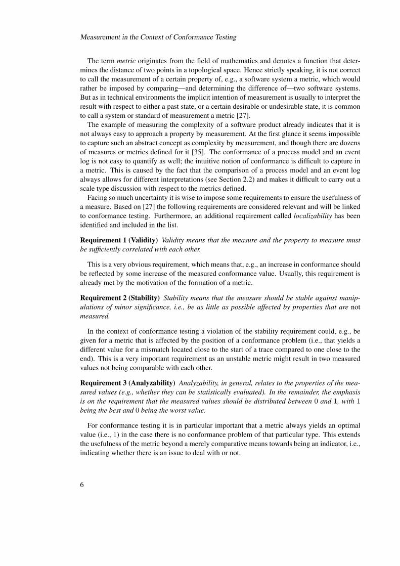
Facing so much uncertainty it is wise to impose some requirements to ensure the usefulness ofa measure. Based on [27] the following requirements are considered relevant and will be linkedto conformance testing. Furthermore, an additional requirement called localizability has beenidentified and included in the list.

Requirement 1 (Validity) Validity means that the measure and the property to measure mustbe sufficiently correlated with each other.

This is a very obvious requirement, which means that, e.g., an increase in conformance shouldbe reflected by some increase of the measured conformance value. Usually, this requirement isalready met by the motivation of the formation of a metric.

Requirement 2 (Stability) Stability means that the measure should be stable against manip-ulations of minor significance, i.e., be as little as possible affected by properties that are notmeasured.

In the context of conformance testing a violation of the stability requirement could, e.g., begiven for a metric that is affected by the position of a conformance problem (i.e., that yields adifferent value for a mismatch located close to the start of a trace compared to one close to theend). This is a very important requirement as an unstable metric might result in two measuredvalues not being comparable with each other.

Requirement 3 (Analyzability) Analyzability, in general, relates to the properties of the mea-sured values (e.g., whether they can be statistically evaluated). In the remainder, the emphasisis on the requirement that the measured values should be distributed between 0 and 1, with 1being the best and 0 being the worst value.

For conformance testing it is in particular important that a metric always yields an optimalvalue (i.e., 1) in the case there is no conformance problem of that particular type. This extendsthe usefulness of the metric beyond a merely comparative means towards being an indicator, i.e.,indicating whether there is an issue to deal with or not.

6

Requirement 4 (Reproducibility) Reproducibility means that the measure should be indepen-dent of subjective influence, i.e., it requires a precise definition of its formation.

Reproducibility is a general requirement calling for a measure being as objective as possible,so that, e.g., different people may arrive at comparable results. This holds also for conformancemetrics.

Requirement 5 (Localizability) Localizability means that the system of measurement formingthe metric should be able to locate those parts in the analyzed object that lack certain desirable(i.e., the measured) properties.

It is very important that a conformance problem is not only reflected by the measured valuebut can also be located, e.g., in the given process model. This is crucial for the business analystas she needs to identify potential points of improvement.

This paper follows the common practice in using the term metric and tries to meet the listedrequirements when defining a metric.

2.2 Interpretation Perspectives

When analyzing discrepancies between two objects it is natural to ask for the cause of the mis-match, if any. For this it is important to keep in mind that every interpretation is (implicitly)based on a certain point of view. As an example imagine two strings being compared with eachother, one missing element in one of them could always be interpreted as an extra element withinthe other. Likewise, this holds for comparing a process model with a set of log traces. Figure 2.2shows a single log trace AC and a process model allowing only for the execution of the sequenceABC, which cannot be directly matched with each other. Depending on the interpretation per-spective two different conclusions may be derived, namely:

1) either the log trace is assumed to be correct and consequently the task B is superfluous inthe model and should be removed,

2) or the model is assumed to be correct and therefore the log event B is considered missingin the log, i.e., B should have been executed.

Figure 2.2: Different conclusions based on a different point of view

7

Interpretation Perspectives

In general the two perspectives are equivalent and their validity depends on the different cir-cumstances in which conformance testing might take place. However, it is important to beconscious of the current view point and its potential implications.

But even if one perspective is fixed, different interpretations regarding the type of error mayarise. For example, an approach to experiment with noise (i.e., erroneously logged or non-loggedevents) is to remove and swap elements of a log trace [28]. The swapping corresponds to thecorrect recording but wrong ordering of the logged events. If one considers removal and swap-ping each as an equally severe root cause for noise, then the application of some conformancemetric evaluating the string distance [26] between the noisy log trace and the correct model pathis not valid for measuring the percentage of noise in the log. The reason for this is that swappingresults in a greater string distance than the removal of one single event as it affects two events(i.e., one needs one insert and one remove operation to compensate the effect).

Since conformance analysis involves a process model representing not one but several po-tential execution sequences, even more different conclusions could be derived. As an exampleconsider Figure 2.3, which is an extension of the example in Figure 2.2. Although it keeps thelog-based perspective, i.e., the log is considered to be correct, there are multiple interpretationspossible, namely:

1a) either task B is considered superfluous and the model is adjusted by removing it,

1b/c) or one might want to extend the behavior of the model by adding either the possibility toskip task B or an alternative path only executing C instead of BC.

Figure 2.3: Different interpretations based on the same log-based perspective

Another example in Figure 2.4 shows that although sticking to the model-based perspective,i.e., the model is considered to be correct, multiple corrective actions are conceivable as well,namely:

2a) either log event B is missing, i.e., B should have been executed,

2b) or log event C is missing, i.e., C should have been executed.

These simple, schematic examples illustrate that a root cause analysis for a mismatch betweenprocess model and event log will always lead to a variety of possible interpretations. Whenapplying conformance analysis techniques to a real business process this can be solved with thehelp of domain knowledge.

8

Figure 2.4: Different interpretations based on the same model-based perspective

2.3 Mapping Model Tasks onto Log Events

An essential preparatory step for performing any kind of conformance analysis is associatingthe tasks in the process model with events in the log file. For this purpose one must abstractfrom the concrete occurrence of a log event (also called audit trail entry), which, assuming atotally ordered log, has a unique position and might carry additional data like, e.g., a time stamp,an originator etc.; to determine log event types. All log events stemming from the same kind ofaction then share the same log event type, which can be thought of as a common label. Therefore,stating that “log event A happened” strictly speaking means that “an instance of log event typeA has occurred”.

Naturally, both the availability of domain knowledge (i.e., understanding the business pro-cess) and proficiency with respect to the enactment technology used (i.e., understanding the logformat) is required to establish the mapping for a real business scenario. On a logical level,however, the following types of mapping between a set of tasks in a model and a set of log eventtypes observed in a log can be identified.

1-to-1 mapping Each task is associated with exactly one type of log event (i.e., a function)and no other task in the model is associated with the same type of log event (i.e., aninjective function). Furthermore, all log events are associated with a modeled task (i.e.,a bijective function). Although activities in real business scenarios take time (i.e., havea start and an end), it is useful to assume one single event (typically this corresponds toa complete1 event) being present for the execution of a task as the minimal informationbeing logged to keep the approach as universal as possible.

In the remainder of this paper the label of a task corresponds to the label of its associatedlog event type.

1-to-0 mapping A task in the model is not logged and thus is not visible in the log, whichis referred to as invisible task. An example for such a task not having a correspondentin the log could be a phone call, which is included as a step in the process definition butnot recorded by the system. With respect to Petri net models, such invisible tasks mightalso be introduced for routing purposes (i.e., to preserve bipartiteness), or emerge from

1The complete event is one of the event type categories referring to the life cycle of an activity, standardized by thecommon XML format for workflow logs used by the ProM framework (refer to http://www.processmining.org forfurther information and the schema definition).

9

Mapping Model Tasks onto Log Events

the conversion from other process model representations, such as Causal matrices [28] orEPCs [17].

In the remainder of this paper invisible tasks are characterized as bearing no label (sincethere is no log event associated) and denoted as a black rectangle.

0-to-1 mapping There is no task associated with the log event, the logged event does notcorrespond to a task in the model.

In the remainder of this paper it is abstracted from this case, assuming that the log has beenpre-processed by deleting all events not having a correspondent in the process model.

1-to-n mapping One task is associated with multiple log events. This happens if the executionof a task is logged at a more fine-grained level, such as recording a task being scheduled,started, and finally completed.

Most information systems provide such detailed information through their logging facil-ities and as a next step one could make use of it to, e.g., explicitly detect parallelism.However, for the time being it is abstracted from this case, assuming that all but one logevent have been discarded.

n-to-1 mapping Multiple tasks in the model are associated with the same type of log event,which are called duplicate tasks. It is important to understand that duplicate tasks onlyemerge from the mapping, since the tasks of a process model themselves are distinguish-able, be it not by means of their label but their identity (which is reflected by their uniqueposition in the graph). The presence of duplicate tasks is very likely for systems loggingthe invocation of an external application for the specific process instance2 but withoutrecording the associated model element (e.g., often models are only used as a referencefor implementing the actual control flow logic). In such a situation, mapping a modelcontaining two alternative paths that invoke the same “archive” application onto a corre-sponding log leads to two duplicate “archive” tasks.

In the remainder of this paper duplicate tasks are characterized as bearing the same label,which corresponds to the label of their—jointly—associated log event type.

As far as terminology is concerned the definitions provided in [2] are respected. In the con-text of Petri net models the term task, being a well-defined step in the process model, is inter-changeably used with the corresponding Petri net term transition. An activity corresponds tothe execution of a task for a specific case by a specific resource, which could be related to theoccurrence of a log event (i.e., an audit trail entry).

2In fact, in ERP systems such as SAP R/3 or PeopleSoft it is often very difficult to even associate the logged eventswith a specific case [19].

10

3 Conformance Metrics

In the course of this section a set of conformance metrics will be defined, using the runningexample introduced in Section 3.1 to motivate the decisions made. Then the existence of twodimensions of conformance, fitness and appropriateness, is emphasized in Section 3.2, and threeapproaches to measure them are presented in Section 3.3 and Section 3.4. Afterwards, an interimevaluation takes place in Section 3.5 and it will turn out that the metrics defined lack certaindesirable properties. Due to this fact two improved appropriateness metrics will be defined inSection 3.6, and a final evaluation of the findings concludes the section in Section 3.7.

3.1 Running Example

The example model used throughout the paper concerns the processing of a liability claim withinan insurance company (see Figure 3.1). It sketches a fictive (but possible real-world) procedureand exhibits typical control flow constructs being relevant in the context of conformance testing.

Figure 3.1: Simplified model of processing a liability insurance claim

At first there are two tasks bearing the same label “Set Checkpoint”. This can be thought of asan automatic backup action within the context of a transactional system, i.e., activity A is carriedout at the beginning to define a rollback point enabling atomicity of the whole process, and atthe end to ensure durability of the results. Then the actual business process is started with thedistinction of low-value claims and high-value claims, which get registered differently (B or C).The policy of the client is checked anyway (D) but in the case of a high-value claim, additionally,the consultation of an expert takes place (G), and then the filed liability claim is being checkedin more detail (H). The two completion tasks E and F can be thought of as two different sub-processes involving decision making and potential payment, taking place in another department.Note that the choice between E and F is influenced by the former choice between B and C, andthe model therefore does not belong to the class of free-choice nets [14].

Figure 3.2 shows three example logs for the process described in Figure 3.1 at an aggregate

11

Two Dimensions of Conformance: Fitness and Appropriateness

level. This means that process instances exhibiting the same event sequence are combined asa logical log trace, memorizing the number of instances to weigh the importance of that trace.That is possible since only the control flow perspective is considered here. In a different settinglike, e.g., mining social networks [5], the resources performing an activity would distinguishthose instances from each other.

Figure 3.2: Three example logs

Note that none of the logs contains the sequence ACGHDFA, although the Petri net modelwould allow this. In fact it is highly probable that a log does not exhibit all possible sequences,since, e.g., the duration of activities or the availability of suitable resources may render somesequences very unlikely to occur. With respect to the example model one could think of task Das a standard task requiring a very low specialization level and task G and H as highly specializedand time-consuming checks, so that finishing G and H before D would be possible but practicallymay not happen. Note that, furthermore, the number of possible sequences generated by aprocess model may grow exponentially, in particular for a model containing concurrent behavior.For example, there are 5! = 120 possible combinations for executing five tasks, and 8! = 40320for executing eight tasks that are parallel to each other.

Therefore, an event log cannot be expected to exhibit all possible sequences of the underlyingbehavioral model. Process mining techniques strive for weakening the notion of completeness,i.e., the amount of information a log needs to contain for being able to rediscover the underlyingprocess model [8].

3.2 Two Dimensions of Conformance: Fitness andAppropriateness

Measurement can be defined as a set of rules to assign values to a real-world property, i.e., obser-vations are mapped onto a numerical scale (see also Section 2.1). In the context of conformancetesting this means to weigh the “distance” between the behavior actually observed in the work-flow log and the behavior described by the process model. If the distance is zero, i.e., the realbusiness process exactly complies with the specified behavior, one can say that the log fits themodel. With respect to the example model M1 this seems to apply for event log L1, since everylog trace can be associated with a valid path from Start to End. In contrast, event log L2 does notmatch completely as the traces ACHDFA and ACDHFA lack the execution of activity G, whileevent log L3 does not even contain one trace corresponding to the specified behavior. SomehowL3 seems to fit “worse” than L2, and the degree of fitness should be determined according to this

12

intuitive notion of conformance, which might vary for different settings.But there is another interesting—rather qualitative—dimension of conformance, which can

be illustrated by relating the process models M2 and M3, shown in Figure 3.3 and Figure 3.4, toevent log L2. Although the log fits both models quantitatively, i.e., the event streams of the logand the model can be matched perfectly, they do not seem to be appropriate in describing theinsurance claim administration.

Figure 3.3: Workflow model on a too high level of abstraction (i.e., too generic)

Figure 3.4: Workflow model on a too low level of abstraction (i.e., too specific)

The first one is much too generic as it covers a lot of extra behavior, allowing for arbitrarysequences containing the activities A, B, C, D, E, F, G, or H, while the latter does not allow formore sequences than those having been observed but only lists the possible behavior instead ofexpressing it in a meaningful way. Therefore, it does not offer a better understanding than canbe obtained by just looking at the aggregated log. One can claim that a “good” process modelshould somehow be minimal in structure to clearly reflect the described behavior, in the follow-ing referred to as structural appropriateness, and minimal in behavior to represent as closely aspossible what actually takes place, which will be called behavioral appropriateness.

Apparently, conformance testing demands for two different types of metrics, which are:

• Fitness, i.e., the extent to which the log traces can be associated with execution pathsspecified by the process model, and

• Appropriateness, i.e., the degree of accuracy in which the process model describes theobserved behavior, combined with the degree of clarity in which it is represented.

13

Measuring Fitness

3.3 Measuring Fitness

As mentioned in Section 2, one way to measure the fit between event logs and process modelsis to replay the log in the model and somehow measure the mismatch, which subsequently isdescribed in more detail. The replay of every logical log trace starts with marking the initialplace in the model and then the transitions that belong to the logged events in the trace arefired one after another. While doing so one counts the number of tokens that had to be createdartificially (i.e., the transition belonging to the logged event was not enabled and therefore couldnot be successfully executed) and the number of tokens that had been left in the model, whichindicates the process not having properly completed.

Metric 1 (Fitness) Let k be the number of different traces from the aggregated log. For eachlog trace i (1 ≤ i ≤ k) ni is the number of process instances combined into the current trace,mi is the number of missing tokens, ri is the number of remaining tokens, ci is the number ofconsumed tokens, and pi is the number of produced tokens during log replay of the current trace.The token-based fitness metric f is formalized as follows:

f =12(1−

∑ki=1 nimi∑ki=1 nici

) +12(1−

∑ki=1 niri∑ki=1 nipi

)

Note that, for all i, mi ≤ ci and ri ≤ pi, and therefore 0 ≤ f ≤ 1. To have a closer look at thelog replay procedure consider Figure 3.5, which depicts the replay of the first trace from eventlog L2 in process model M1. At the beginning (a) one initial token is produced for the Start placeof the model (p = 1). The first log event in the trace, A, is associated with two transitions inthe model (each bearing the label A—according to Section 2.3 they are called duplicate tasks).However, only one of them is enabled and thus will be fired (b), consuming the token from Startand producing one token for place c1 (c = 1, p = 2). Now the next log event can be examined.The corresponding transition B is enabled and can be fired (c), consuming the token from c1and producing one token each for c2 and c5 (c = 2, p = 4). Then, the following log eventcorresponds to transition D, which is enabled and therefore can be fired (d), consuming the tokenfrom c2 and producing a token for c3 (c = 3, p = 5). Similarly, the transition associated to thenext log event E is also enabled and fired (e), consuming the token from c3 and c5, and producingone token for c4 (c = 5, p = 6). Finally, the last log event is of type A again, i.e., is associatedwith the two transitions A in the model. But once more only one of them is enabled and thereforechosen to be fired (f), consuming the token from c4 and producing one token for the End place(c = 6, p = 7). As a last step this token at the End place is consumed (c = 7) and the replayfor that trace is completed. There were neither tokens missing nor remaining (m = 0, r = 0),i.e., this trace is perfectly fitting the model M1. Similarly, the second and third trace can also beperfectly replayed, i.e., neither tokens are missing nor remaining (m2 = m3 = r2 = r3 = 0).

Now consider Figure 3.6, which depicts the replay of the fourth trace from event log L2 inM1. At the beginning (a)(b) the procedure is very similar, only that—instead of transition B—transition C is fired (c), consuming the token from c1 and producing one token each for c2 andc6 (c = 2, p = 4). But examining the next log event it turns out that its corresponding transitionH is not enabled. Consequently, the missing token in c7 is artificially created and recorded

14

Figure 3.5: Log replay for trace i = 1 of event log L2 in process model M1

15

Measuring Fitness

Figure 3.6: Log replay for trace i = 4 of event log L2 in process model M1

16

(m = 1), and the transition is fired (d), consuming it and producing one token for place c8(c = 3, p = 5). In contrast, the following log events can be successfully replayed again, i.e.,their associated transitions are enabled and can be fired: (e) transition D consumes the tokenfrom c2 and produces one token for c3 (c = 4, p = 6), (f) transition F consumes the token fromc8 and c3 and produces one token for c4 (c = 6, p = 7), (g) one of the two associated transitionsA is enabled and can be fired, consuming the token from c4 and producing one token for theEnd place (c = 7, p = 8). At last the token at the End place is consumed again (c = 8). Butthen there is still a token remaining in place c6, which will be punished as it indicates that theprocess did not complete properly (r = 1). A similar problem will be encountered replaying thelast trace of event log L2. Again, the model M1 requires the execution of task G but this did nothappen, and therefore a token is remaining in place c6 (r5 = 1) and a token is missing in placec7 (m5 = 1).

Using the metric f one can now calculate the fitness between the whole event log L2 andthe process description M1. As stated before, besides trace i = 4 only the last log tracei = 5 had tokens missing and remaining. Counting also the number of tokens being pro-duced and consumed while replaying the other three traces (i.e., c2 = c3 = p2 = p3 = 9,and c5 = p5 = 8), and with the given number of process instances per trace, the fitness canbe measured as f(M1, L2) = 1 − 23+28

(1207·7)+((145+56)·9)+((23+28)·8) ≈ 0.995. Similarly, onecan calculate the fitness between the event logs L1, L3, and the process description M1, respec-tively. The first event log L1 shows three different log traces that all correspond to possiblefiring sequences of the Petri net with one initial token in the Start place. Thus, there are nei-ther tokens left nor missing in the model during log replay and the fitness measurement yieldsf(M1, L1) = 1. In contrast, for the last event log L3 none of the traces can be associated witha valid firing sequence of the Petri net and the fitness measurement yields f(M1, L3) ≈ 0.540.

Figure 3.7: Diagnostic token counters provide insight into the location of errors

Besides measuring the degree of fitness pinpointing the site of mismatch is crucial for givinguseful feedback to the analyst. In fact, the place of missing and remaining tokens during logreplay can provide insight into problems, such as Figure 3.7 visualizes some diagnostic infor-mation obtained for event log L2. Because of the remaining tokens (whose amount is indicatedby a + sign) in place c6 transition G has stayed enabled, and as there were tokens missing (indi-cated by a − sign) in place c7 transition H has failed seamless execution. Regarding evaluationof potential alignment procedures, the model rather lacks the possibility to skip activity G thanthat the expert consultation would be considered missing in almost half of the high-value claimsthat took place; however, a final interpretation could only be given by a domain expert from the

17

Measuring Appropriateness

insurance company.Note that this replay is carried out in a non-blocking way and from a log-based perspective,

i.e., for each log event in the trace the corresponding transition is fired, regardless whether thepath of the model is followed or not. This leads to the fact that—in contrast to directly comparingthe event streams of models and logs—a concatenation of missing log events is punished by thefitness metric f just as much as a single one, since it could always be interpreted as a missinglink in the model.

As described in Section 2.3, a prerequisite for conformance analysis is that modeled tasksmust be associated with the logged events, which may result in duplicate tasks, i.e., multipletasks that are mapped onto the same type of log event, and invisible tasks, i.e., tasks that have nocorresponding log event. Duplicate tasks cause no problems during log replay as long as they arenot enabled at the same time and can be executed (like shown in Figure 3.5 and Figure 3.6 for thetwo tasks labeled as A), but otherwise one must enable and/or fire the right task for progressingproperly. Invisible tasks are considered to be lazy [28], i.e., they are only fired if they can enablethe transition in question. In both cases it is necessary to partially explore the state space, whichis described in more detail in Section 4.3.

3.4 Measuring Appropriateness

Generally spoken, determining the degree of appropriateness of a workflow process modelstrongly depends on subjective perception, and is highly correlated to the specific purpose.There are aspects like the proper semantic level of abstraction, i.e., the granularity of the de-scribed workflow actions, which can only be found by an experienced human designer. Thenotion of appropriateness addressed by this paper rather relates to the control flow perspectiveand therefore can be measured, although the measurement has a subjective element.

Figure 3.8: Model appropriate in structure and behavior

The overall aim is to have the model clearly reflect the behavior observed in the log, whereasthe degree of appropriateness is determined by both structural properties of the model and thebehavior described by it. Figure 3.8 shows M4, which appears to be a good model for the eventlog L2 as it exactly generates the observed sequences in a structurally suitable way.

In the remainder of this section, both the structural and the behavioral part of appropriatenessare considered in more detail.

18

3.4.1 Structural Appropriateness

The desire to model a business process in a compact and meaningful way is difficult to captureby measurement. As a first indicator a simple metric solely based on the graph size of the modelwill be defined, and subsequently some constructs that may inflate the structure of a processmodel are considered.

Metric 2 (Structural Appropriateness) Let L be the set of labels, and N the set of nodes (i.e.,places and transitions) in the Petri net model, then the structural appropriateness metric aS isformalized as follows:

aS =|L|+ 2|N |

As described in Section 2.3 the mapping between modeled tasks and logged events is repre-sented by a label denoting the associated log event type (if any) for each task. Given the fact thata business process model is expected to have a dedicated Start and End place (see the WF-netrequirements in Section 2), the graph must contain at least one transition for every task label,plus two places (the start and end place). In this case |N | = |L|+ 2 and the metric aS yields thevalue 1. The more the size of the graph is growing, e.g., due to additional places, the measuredvalue moves towards 0.

Calculating the structural appropriateness for the model M3 yields aS(M3) ≈ 0.170, which isa very bad value caused by the many duplicate tasks (as they increase the number of transitionswhile having identical labels). For the good model M4 the metric yields aS(M4) = 0.5. WithaS(M5) ≈ 0.435 a slightly worse value is calculated for the behaviorally (trace) equivalentmodel in Figure 3.9, which is now used to consider some constructs that may decrease thestructural appropriateness aS .

Figure 3.9: Structural properties may reduce the appropriateness of a model

(a) Duplicate tasks. Duplicate tasks that are used to list alternative execution sequences tendto produce models like the extreme M3. Figure 3.9 (process model M5) shows an examplesituation in which a duplicate task is used to express that after performing activity C either thesequence GH or H alone can be executed (see (a) in Figure 3.9). Figure 3.8 (process model M4)describes the same process with the help of an invisible task (see (b) in Figure 3.8), which isonly used for routing purposes and therefore not visible in the log. One could argue that thismodel supports a more suitable perception namely activity G is not obliged to execute but can

19

Measuring Appropriateness

be skipped, but it somehow remains a matter of taste. However, excessive usage of duplicatetasks for listing alternative paths reduces the appropriateness of a model in preventing desiredabstraction.

In addition, there are also duplicate tasks that are necessary to, e.g., specify a certain activitytaking place exactly at the beginning and at the end of the process like task A in process modelM4 (see (a) in Figure 3.8).

(b) Invisible tasks. Besides the invisible tasks used for routing purposes like, e.g., shown by(b) in Figure 3.8, there are also invisible tasks that only delay visible tasks, such as the one in-dicated by (b) in Figure 3.9. If they do not serve any model-related purpose they can simply beremoved, thus making the model more concise.

(c) Implicit places. Implicit places are places that can be removed without changing thebehavior of the model [8]. An example for an implicit place is given by place c10 (see (c)in Figure 3.9). Again, one could argue that they should be removed as they do not contributeanything, but sometimes it can be useful to insert such an implicit place to, e.g., show documentflows.

Note that the place c5 in Figure 3.9 is not implicit as it influences the choice made later onbetween E and F. Both c5 and c10 are silent places, with a silent place being a place whosedirectly preceding transitions are never directly followed by one of their directly succeedingtransitions (e.g., for M4 it is not possible to produce an event sequence containing BE or AA).Mining techniques by definition are unable to detect implicit places, and have problems detectingsilent places.

3.4.2 Behavioral Appropriateness

Besides the structural properties that can be evaluated on the model itself appropriateness canalso be examined with respect to the behavior recorded in the log. Assuming that the log fitsthe model, i.e., the model allows for all the execution sequences present in the log, there remainthose that would fit the model but have not been observed. Assuming further that the log satisfiessome notion of completeness, i.e., the behavior observed corresponds to the behavior that shouldbe described by the model, it is desirable to represent it as precisely as possible. When the modelgets too general and allows for more behavior than necessary/likely (like in the “flower” modelM2) it becomes less informative in actually describing the process.

One approach to measure the amount of possible behavior is to determine the mean numberof enabled transitions during log replay. This corresponds to the idea that for models clearlyreflecting their behavior, i.e., complying with the structural properties mentioned above, an in-crease of alternatives or parallelism and therefore an increase of potential behavior will result ina higher number of enabled transitions during log replay.

Metric 3 (Behavioral Appropriateness) Let k be the number of different traces from the ag-gregated log. For each log trace i (1 ≤ i ≤ k) ni is the number of process instances combinedinto the current trace, and xi is the mean number of enabled transitions during log replay ofthe current trace (note that invisible tasks may enable succeeding labeled tasks but they are not

20

counted themselves). Furthermore, m is the number of labeled tasks (i.e., does not include invis-ible tasks, and assuming m > 1) in the Petri net model. The behavioral appropriateness metricaB is formalized as follows:

aB = 1−∑k

i=1 ni(xi − 1)

(m− 1) ·∑k

i=1 ni

Calculating the behavioral appropriateness with respect to event log L2 for the model M2yields aB(M2, L2) = 0, which indicates the arbitrary behavior described by it. For M4, whichexactly allows for the behavior observed in the log, the metric yields aB(M4, L2) ≈ 0.967. Asan example it can be compared with the model M6 in Figure 3.10, which additionally allows forarbitrary loops of activity G and therefore exhibits more potential behavior. This is also reflectedin the behavioral appropriateness measure as it yields a slightly smaller value than for the modelM4, namely aB(M6, L2) ≈ 0.964.

Figure 3.10: Unnecessary potential behavior may reduce the appropriateness of a model

3.5 Balancing Fitness and Appropriateness—an InterimEvaluation

Having defined the three metrics f , aS , and aB , the question is now how to put them together.This is not an easy task since they are partly correlated with each other. So the structure of aprocess model may influence the fitness metric f as, e.g., due to inserting redundant invisibletasks the value of f increases because of the more tokens being produced and consumed whilehaving the same amount of missing and remaining ones. But unlike aS and aB the metric fdefines an optimal value 1.0, for a log that can be parsed by the model without any error.

Therefore, it is recommended to carry out the conformance analysis in two phases. Duringthe first phase the fitness of the log and the model is ensured, which means that discrepanciesare analyzed and potential corrective actions are undertaken. If there still remain some tolerabledeviations, the log or the model should be manually adapted to comply with the ideal or intendedbehavior, in order to go on with the so-called appropriateness analysis. Within this second phasethe degree of suitability of the respective model in representing the process recorded in the logis determined.

21

Balancing Fitness and Appropriateness—an Interim Evaluation

Table 3.1: Diagnostic results

M1 M2 M3 M4 M5 M6f = 1.0 f = 1.0 f = 1.0 f = 1.0 f = 1.0 f = 1.0

L1 aS = 0.5263 aS = 0.7692 aS = 0.1695 aS = 0.5 aS = 0.4348 aS = 0.5556aB = 0.9740 aB = 0.0 aB = 0.9739 aB = 0.9718 aB = 0.9749 aB = 0.9703a = 0.5126 a = 0.0 a = 0.1651 a = 0.4859 a = 0.4239 a = 0.5391f = 0.9952 f = 1.0 f = 1.0 f = 1.0 f = 1.0 f = 1.0

L2 aS = 0.5263 aS = 0.7692 aS = 0.1695 aS = 0.5 aS = 0.4348 aS = 0.5556aB = 0.9705 aB = 0.0 aB = 0.9745 aB = 0.9669 aB = 0.9706 aB = 0.9637

a = 0.0 a = 0.1652 a = 0.4835 a = 0.4220 a = 0.5354f = 0.5397 f = 1.0 f = 0.4947 f = 0.6003 f = 0.6119 f = 0.5830

L3 aS = 0.5263 aS = 0.7692 aS = 0.1695 aS = 0.5 aS = 0.4348 aS = 0.5556aB = 0.8909 aB = 0.0 aB = 0.8798 aB = 0.8904 aB = 0.9026 aB = 0.8894

Regarding the example logs given in Figure 3.2 this means that an evaluation of the appro-priateness measurements takes place only for those models having a fitness value f = 1.0 (cf.Table 3.1) and therefore event log L3, which only fits the trivial process model M2, is com-pletely discarded, just like process model M1 for event log L2. For event logs L1 and L2 nowthe most adequate process model should be found among the remaining ones, respectively. Forthis purpose a simple appropriateness metric, combining the structural and the behavioral partas a product (i.e., denoting the area within the unit square), is defined.

Metric 4 (Appropriateness) Based on the structural appropriateness metric aS and the behav-ioral appropriateness metric aB the unified appropriateness metric a is defined as follows:

a = aS · aB

Examining the values of the unified appropriateness metric a in Table 3.1 it turns out that themodel M6 is selected as the most appropriate representation for the behavior observed in boththe event log L1 and L2, which is not in line with intuitive expectations. While looking for ananswer, one can observe that for the extremely generic model M2 the aS value is always veryhigh while the aB value is very low and vice versa for the extremely specific model M3. Sofor finding the most appropriate process model it seems like both the structural appropriatenessmetric aS and the behavioral appropriateness metric aB must be understood as an indicator tobe maximized without decreasing the other. However, balancing them will always be difficultas they are correlated with each other, which becomes clear reconsidering the assumptions themetrics are based on.

The motivation for measuring the amount of potential behavior via the mean number of en-abled transitions during log replay was explicitly based on the assumption that the structure ofthe process model clearly reflects the behavior which is expressed by it. This means that themetric aB is limited in its applicability, since the fundamental idea that adding alternative or

22

parallel behavior to a Petri net will increase the mean number of enabled transitions during logreplay only holds for a certain class of process models. As soon as a process model is stronglysequentialized using alternative duplicate tasks, such as it is the case for the extremely specificmodel M3, the assumption does not hold anymore and the result becomes meaningless. Onecan further observe that the model M4 yields a worse aB value than the model M5 althoughthey are behaviorally (trace) equivalent. This shows that the metric aB is affected by structuralproperties, which violates the stability requirement (see Requirement 2 in Section 2.1).

But also the metric aS , which should only measure the structural appropriateness, is not in-dependent of the behavioral expressiveness of a model. The very good aS value for processmodel M2 shows that it is easy to make a model more compact while rendering it more genericin behavior. Imagine a natural language where (for any reason such as faster speaking, or a lackof space in writing) the suitability of using a word is based on the number of letters it is formedof. The shorter word among two words can then, however, only be considered the better if theyboth mean the same. Following this analogy, there is the implicit assumption that it makes onlysense to compare models based on their graph size if they somehow allow for the same amountof behavior (which violates the stability requirement, too).

Revising the other requirements imposed in Section 2.1 one will detect that also the analyz-ability requirement (see Requirement 3) is not fulfilled with respect to aS and aB . The measuredvalues do not seem to be very well distributed (note that the behavioral appropriateness valueaB , except for the extreme M2, is always around 0.96 or 0.97 with respect to L1 and L2), andalthough it is possible to reach the optimal value 1 this is not guaranteed for an optimal solution.For example, one would expect the process model M1 having an optimal structure, as a morecompact representation of the behavior specified does not seem feasible. However, the structuralappropriateness aS(M1) only yields 0.5263. Similarly, model M4 precisely specifies the behav-ior observed in event log L2, but still aB(M4, L2) only yields 0.9669, which suggests that therewould be a better solution.

As a comparative means and within the class of process models where their respective as-sumptions are fulfilled, the presented metrics can be very well applied. So can the aS metric beused to find out that the process model M4 corresponds to a structurally more suitable represen-tation than M3 and M5. The aB metric determines M1, the initial Petri net given in Figure 3.1,as the behaviorally most suitable model over M2, M4, and M6 for the event log L1. Similarly,M4 is considered behaviorally more suitable than M2 or M6 for event log L2.

However, to extend the applicability it would be useful to have an independent measure forboth structural and behavioral appropriateness, i.e., meeting Requirement 2, and to also reach anoptimal point, indicating that there is no better solution available, i.e., meeting Requirement 3.

3.6 Alternative Approaches for Measuring Appropriateness

Based on the insight gained into the weak points of the appropriateness metrics defined so farthe aim is now to find alternative metrics, which are independent (i.e., not affected by propertiesthat should not be measured) and better distribute possible values between 0 and 1 (in particulardefine an optimal value). In the following an alternative approach for both measuring structural

23

Alternative Approaches for Measuring Appropriateness

and behavioral appropriateness is presented.

3.6.1 Structural Appropriateness

When defining a metric for measuring structural appropriateness one might be tempted to favora specific behavioral pattern [3], e.g., the Sequence, over others, for reasons such as approxi-mating the most common behavior or just to ”make the examples work”. But actually, structuremust be seen as the syntactic means by which behavior (i.e., the semantics) may be specifiedat all. When using Petri nets to model business processes like every language this is formedby the vocabulary (i.e., places, transitions, and edges) combined with a set of rules (such as thebipartiteness requirement).

Often there are several syntactic ways to express the same behavior and the challenge of astructural appropriateness metric is to verify certain design guidelines, which define the pre-ferred way to express a certain behavioral pattern, and to somehow punish their violations. Itis obvious that these design guidelines will vary for different process modeling notations andmay depend on personal or corporate preferences. However, to demonstrate the character of anindependent structural appropriateness metric the findings of Section 3.4.1 will be used to definean alternative metric a′S . As a design guideline, constructs such as alternative duplicate tasksand redundant invisible tasks should be avoided as they were identified to inflate the structure ofa process model and to detract from clarity in which the expressed behavior is reflected.

As the definition of these constructs requires an analysis of the state space of the processmodel, some preparative definitions are provided in the following.

Definition 1 (Labeled Transition System) A labeled transition system is defined as TS =(S, E, T, L, l) where S is the set of states, E ⊆ (S × T × S) is the set of state transitions,T the set of transition names, L a set of transition labels, and l ∈ T 6→ L is a partial labelingfunction (only the transitions in dom(l) are visible). It is assumed to have a unique start stateStart and end state End.

Definition 2 (Paths and Projection) Given a labeled transition system TS = (S, E, T, L, l):

• paths(TS) ⊆ T ∗ is the set of paths in TS (a path p being defined as a sequence of lengthlen(p), i.e., p = (p0, . . . , plen(p)−1)) starting in state Start and ending in state End,

• for all p ∈ paths(TS), proj(p) is the projection of p onto L, i.e., visible transitions arerelabeled using l while invisible transitions are removed, and

• projection(TS) = {proj(p) | p ∈ paths(TS)}.

A labeled transition system TS will be used to represent the state space of the process model.Then paths(TS) denotes the set of possible execution sequences with respect to that modelwhile projection(TS) represents the set of traces that could be possibly observed in a log (as,like stated in Section 2.3, the label serves as a mapping between modeled tasks and log events).

Now the alternative duplicate tasks and redundant invisible tasks are defined and the alterna-tive metric a′S is presented.

24

Definition 3 (Alternative Duplicate Tasks) Let TS = (S, E, T, L, l) be the labeled transitionsystem denoting the state space of a Petri net model, and Dlab the set of duplicate tasks bearingthe same label lab, then the set of Alternative Duplicate Tasks DA is defined as follows:

AlabD = {(x, y) ∈ Dlab ×Dlab | ¬∃p∈paths(TS) (∃0≤i<j<len(p) ((x 6= y) ∧ (3.1)

((pi = x ∧ pj = y) ∨ (pi = y ∧ pj = x))))}, lab ∈ L

DlabA =

{∅ if Alab

D = ∅Dlab if Alab

D 6= ∅ , lab ∈ L (3.2)

DA =⋃

lab∈L

DlabA (3.3)

Equation 3.1 defines a relation AlabD over the cross product of a set of equally labeled tasks

Dlab, selecting those pairs that are never contained together in one possible execution path,i.e. are alternative to each other. Only different transitions are considered, and therefore setsDlab with only one transition contained (i.e., non-duplicates) will result in Alab

D = ∅. A set ofduplicate tasks containing more than two transitions is considered alternative as soon as thereare two tasks contained that are alternative to each other. This is reflected by Equation 3.2 aseither Dlab

A = Dlab, if the corresponding alternative duplicates relation AlabD is not empty, or is

set to the empty set. Finally, in Equation 3.3 all the sets of alternative duplicate tasks from theprocess model are merged, which is denoted by DA.

Note that according to the definition the duplicate tasks indicated by (a) in Figure 3.8 are notalternative, and therefore are not contained in DA.

Definition 4 (Redundant Invisible Tasks) Let TS = (S, E, T, L, l) be the labeled transitionsystem denoting the state space of a Petri net model, and I the set of invisible tasks (i.e., I ={t ∈ T | t 6∈ dom(l)}). Given TS and a t ∈ T : merge(TS, t) is the labeled transitionsystem resulting from merging the source and target nodes of all edges referring to t, i.e., forany (s1, t, s2) ∈ E, states s1 and s2 are merged. The set of Redundant Invisible Tasks IR isdefined as follows:

IR = {t ∈ I | projection(TS) = projection(merge(TS, t))} (3.4)

The idea behind a redundant invisible task is that it can somehow be removed from the modelwithout affecting the set of possibly generated traces, i.e., the projection. Since defining thisproperty on the graph level (i.e., the Petri net level) is a bit more involved, the definition makesuse of merging states in the corresponding transition system, such that the specific transition isnot contained anymore. Then in Equation 3.4 for each invisible task of the model is checkedwhether the set of possible traces of the modified transition system is the same as for the initialtransition system. If so, the task is considered redundant and thus included into IR.

According to this definition the invisible task contained in model M4 (see (b) in Figure 3.8)is not redundant as via merging its source and target states the corresponding labeled transitionsystem would additionally allow for traces containing arbitrary sequences of G.

25

Alternative Approaches for Measuring Appropriateness

Another requirement is covered by the implicit assumption that the transition system resultingfrom the merge operation must still have a unique Start start and a unique End state. The reasonfor this is that, e.g., the invisible tasks contained in model M2 are not redundant as removingthem would lead to a process model without having a dedicated Start and End place, i.e., itwould not be a WF-net anymore.

Metric 5 (Improved Structural Appropriateness) Let T be the set of transitions in the Petrinet model, then the improved structural appropriateness metric a′S is formalized as follows:

a′S =|T | − (|DA|+ |IR|)

|T |

Note that |DA|+ |IR| ≤ |T | and therefore 0 ≤ a′S ≤ 1 as duplicate tasks are always visible.Revising the example models it turns out that, according to the defined design guideline, onlymodel M5 and M3 are reduced in structural appropriateness. For M5 the number of alternativeduplicate tasks |DA| = 2 (see (a) in Figure 3.9) and the number of redundant invisible tasks|IR| = 1 (see (b) in Figure 3.9), which results in a′S(M5) ≈ 0.727. In M3 all tasks but B belongto the set of alternative duplicate tasks and therefore a′S(M3) ≈ 0.032.

Figure 3.11: Design guideline violations can be visualized

Finally, a very important point is that building a notion of structural appropriateness with thehelp of some kind of design guideline usually enables the visualization of its violations (see Fig-ure 3.11). This demonstrates that metric a′S—in contrast to metric aS—meets the localizabilityrequirement (see Requirement 5 in Section 2.1).

3.6.2 Behavioral Appropriateness

To approach behavioral appropriateness independently from structural properties the potentialbehavior specified by the model will be analyzed and compared with the behavior actuallyneeded to describe what has been observed in the log. In order to somehow measure their“distance” a set of relations can be derived from both the process model (analyzing the possibleexecution sequences) and the event log (analyzing the observed execution sequences). When re-ferring to the traces generated by the process model Definition 2 and Definition 1 from Section3.6.1 will be reused.

26

Definition 5 (Always and Never Relation Forwards and Backwards) Let L be the set of alllabels (including an artificially inserted Start and End task or log event, respectively). PL is ei-ther projection(TS) for TS representing the labeled transition system for the process model orthe set of all traces contained in the event log, respectively. The Always Relation Forwards AF ,the Never Relation Forwards NF , the Always Relation Backwards AB , and the Never RelationBackwards NB are formalized as follows:

PL(x) = {p ∈ PL | ∃0≤i<len(p) pi = x}, x ∈ L (3.5)

AF = {(x, y) ∈ L× L | (3.6)

(PL(x) 6= ∅) ∧ (∀p∈PL(x) (∃0≤i<j<len(p) (pi = x ∧ pj = y)))}NF = {(x, y) ∈ L× L | ¬∃p∈PL

(∃0≤i<j<len(p) (pi = x ∧ pj = y))} (3.7)

AB = {(x, y) ∈ L× L | (3.8)

(PL(x) 6= ∅) ∧ (∀p∈PL(x) (∃0≤j<i<len(p) (pi = x ∧ pj = y)))}NB = {(x, y) ∈ L× L | ¬∃p∈PL

(∃0≤j<i<len(p) (pi = x ∧ pj = y))} (3.9)

As discussed in Section 2.3 in the scope of this paper the set of labels L serves as a linkbetween the model task identifiers and the elements contained in the log, denoting the mappingthat has been established. Furthermore, it was assumed that log events not referring to any taskin the model were removed from the log. In doing so it is possible to derive comparable relationsfrom both the model and the log perspective.

While building the relations for the model recall that invisible tasks are defined unlabeled andthus are not covered by L. What is more, duplicate tasks bear the same label and consequentlyare represented only once within L. This leads to the fact that if there are three duplicate tasksx1, x2, and x3 jointly labeled with x the expressions involving x decompose to x1 ∨ x2 ∨ x3,i.e., the successor or predecessor relationship between two label elements is acknowledged assoon as it holds for any of the duplicates. Clearly during this projection some information islost, namely which precise task was considered successor or predecessor, but this is logicallyconsistent as the relations will be verified with respect to the log, which does not allow for thisdistinction either.

Note that the successor relationship (cf. Forwards relations) and the predecessor relationship(cf. Backwards relations) are defined globally, i.e., are acknowledged as soon as they hold forany pair of labels. To give an example imagine a path p = (. . . , x, . . . , x, . . . , y, . . . , x, . . .).Here the global successor-ship would be confirmed for the tuple (x, y) although it does not holdfor all x that it is followed by y, and although they do not directly follow each other. Thisis motivated by the desire to also capture global behavioral dependencies, which, e.g., may beintroduced by non-free-choice constructs [14], and to recognize a behavioral constraint that onlyinvolves one transition out of a set of duplicate tasks.

Note further that the insertion of an artificial Start and End task (or log event, respectively) isonly needed to capture the special case of alternative paths leading directly from the Start placeto the End place of the model, and therefore can be left out if this does not apply.

27

Alternative Approaches for Measuring Appropriateness

Definition 6 (Sometimes Relation Forwards and Backwards) Let L be the set of all labels(including an artificially inserted Start and End task or log event, respectively), then the Some-times Relation Forwards SF and the Sometimes Relation Backwards SB are formalized as fol-lows:

SF = (L× L) \ (AF ∪NF ) (3.10)

SB = (L× L) \ (AB ∪NB) (3.11)

Based on the previously defined relations AF and NF the relation SF can be defined (seeEquation 3.10). Together they state for each pair of labels (x, y) whether y either always, ornever, or sometimes follows x; with respect to the set possible execution paths (model perspec-tive) or the set of log traces (log perspective), correspondingly. Analogously SB is defined viaAB and NB (see Equation 3.11), intuitively stating for each pair of labels (x, y) whether y ei-ther always, or never, or sometimes precedes x. Note that due to the additional requirementPL(x) 6= ∅ in Equation 3.6 AF , NF , and SF indeed partition L × L. Similarly, AB , NB , andSB partition L × L due to Equation 3.8. PL(x) is empty if log event x has not been observedas, e.g., an alternative branch has always been decided in the same way (and therefore the tasklabeled x has never been executed). If the requirement was dropped, in such a case all the tuples(x, ...) were contained in both relation AF and relation NF (the same holds for AB and NB).However, as the formation of the new behavioral appropriateness metric later in this section willonly be based on the relations SF and SB the requirement is not really necessary and rather wasadded in order to correspond to intuition.

Figure 3.12: Deriving the “footprint” from a process model

28

Together the defined relations can be considered being a (left and a right) “footprint” (see alsoFigure 2.1) of the behavior represented. As an example, consider Figure 3.12 where the For-wards relations and the Backwards relations are derived for the process model M4 and depictedin the F matrix and B matrix, respectively.

Both the SF and SB relation are highlighted as they indicate concurrent or alternative behav-ior. Parallel tasks may follow each other in any order, such that (D,G), (D,H), (G, D), and(H,D) are contained in both relation SF and relation SB . Alternative paths are also reflected bytuples contained in the Sometimes relations: Tasks preceding an alternative branch can be fol-lowed by any of the alternative paths, and therefore—together with the tasks contained in thosepaths—form part of the Sometimes Relation Forwards, i.e., (Start,B), (Start, E), (Start, C),(Start,G), (Start,H), (Start, F ), (A,B), (A,E), (A,C), (A,G), (A,H), (A,F ), (C,G),(D,E), and (D,F ) ∈ SF . Similarly, the tasks succeeding the alternative join can be pre-ceded by any of the alternative paths, and therefore—together with the tasks contained in thosepaths—form part of the Sometimes Relation Backwards, i.e., (End,E), (End,B), (End, F ),(End,H), (End,G), (End,C), (A,E), (A,B), (A,F ), (A,H), (A,G), (A,C), (H,G),(D,B), and (D,C) ∈ SB .

Note that this asymmetry with respect to alternative behavior is also the motivation for in-cluding both directions in the improved behavioral appropriateness metric that will be definedlater on in this section. If one would only evaluate one of them, the position of, e.g., an unusedalternative path in the model (such as close to the Start place or close to the End place) wouldaffect the measured value, which would violate Requirement 2 from Section 2.1.

Figure 3.13: Matching the model “footprint” with the one from the log

29

Alternative Approaches for Measuring Appropriateness

Now consider Figure 3.13, where the S relations of the model in Figure 3.12 have beenmatched with the “footprint” of the log L1. Note that it is sufficient to compare the elementsderived from the S relations of the model with the corresponding tuples of the relations derivedfrom the log. For evaluating behavioral appropriateness it is solely relevant to find out in whichplace the log becomes more specific, i.e., the model allows for more behavior than necessary. InFigure 3.13 this is the case for two tuples each in the SF and in the SB relation.

First, the tuple (H,D) becomes an element of the NF relation (instead of SF ), and (H,D)becomes an element of AB (instead of SB), which is caused by the fact that, although accordingto the model task D and H are concurrent and could be executed in any order, finishing D after Hhas never happened. Second, the tuple (C,G) becomes an element of the AF relation (insteadof SF ) and (H,G) becomes an element of AB (instead of SB). This is caused by the fact thatthe process model allows to skip activity G, which has never been used by the process observedin event log L1.

Apparently, this behavioral appropriateness analysis approach is able to highlight unused al-ternative and concurrent behavior, which can also be visualized in some way (see Figure 3.14).This demonstrates that it—in contrast to the approach presented in Section 3.4.2—meets thelocalizability requirement (see Requirement 5 in Section 2.1).

Figure 3.14: Restricted relationships can be visualized

However, interpretation of these results may vary and can only be accomplished by a domainexpert as for analysis the log is assumed to be complete1, i.e., to somehow exhibit all the behaviorthat can happen according to the underlying process model. Like already discussed in Section 3.1this is not necessarily the case.

According to the example process observed in event log L1 task D and task H are not exe-cuted in parallel. However, the control flow of a process model represents causal dependencies,i.e., a partial ordering, among a set of tasks. Therefore, a possible interpretation could be thatthey are not causally related to each other, i.e., they are concurrent from a modeling point ofview. Consequently, the indicated problem results from the log not being complete. Similarly,

1Note that the notion of completeness applied here corresponds to a slightly weaker assumption than the definitionprovided in [8] in the context of process mining. They both do not require all possible sequences being present inthe log (which, as already discussed, would be a very strong assumption) but call for every two tasks that poten-tially follow each other to actually do so in some trace. The notion assumed for this behavioral appropriatenessapproach is slightly weaker in the sense that the successor-ship property is evaluated globally instead of assumingthe events directly following each other.

30

the possibility to skip activity C was not used while handling more than 4300 instances but stillcould be interpreted as a rare exceptional behavior, which has not been observed. This indicatesthat completeness is a problem inherent to any behavioral appropriateness approach, and that afinal interpretation of the results obtained can only be given by an experienced business analyst.

The improved approach to quantify behavioral appropriateness is based on the cardinal num-bers of the Sometimes relations, which corresponds to the idea that increasing the potentialbehavior of a model, i.e., adding alternatives or concurrency, will lead to an increased numberof elements being contained in SF and/or SB .

Metric 6 (Improved Behavioral Appropriateness) Let L be the set of all labels (including anartificially inserted Start and End task or log event, respectively), max = |L|2 − 3|L| + 2, Sm

F

the SF relation and SmB the SB relation for the process model, and Sl

F the SF relation and SlB

the SB relation for the event log (assuming |SlF | < max and |Sl

B| < max), then the improvedbehavioral appropriateness metric a′B is defined as follows:

a′B =12(

max− |SmF |

max− |SlF ∩ Sm

F |) +

12(

max− |SmB |

max− |SlB ∩ Sm

B |)

The value max = |L|2 − 3|L| + 2 has been assigned as the artificially inserted Start andEnd task or log event, respectively, do not allow for certain relations, and therefore a valuemax = |L × L| could never be reached. Note further that, building the intersection of Sl

F andSm

F , and SlB and Sm

B , respectively, tuples contained in the sometimes relations of the log but notin those of the model (which can only happen if the log does not fit the model) are discarded andtherefore the values assigned by a′B range from 0 to 1.

Applying metric a′B to the example yields a′B(M4, L1) = 72−1872−16 ≈ 0.964. This value can be

compared to a′B(M1,M1) = 72−1872−17 ≈ 0.982, which is better as the process model M1 is—due

to the lack of possibility for omitting activity G—considered behaviorally more specific, andthus more appropriate, with respect to event log L1 than process model M4. In fact, M1 is eventhe best model for event log L1 and the reason for a′B(M1, L1) < 1.0 could be for instance thatthe log is incomplete (i.e., H has never been followed by D although this would be possible).

However, the strength of the presented approach lies in its weak notion of completeness,which, e.g., allows to recognize concurrent behavior even if not all possible interleavings ofparallel tasks are represented in the log. As an example, L2 is complete (and thus a′B(M4, L2)yields 1.0) although the possible trace ACGHDFA is not present either.

3.7 Final Evaluation

Having defined two alternative appropriateness metrics a′S and a′B they can now be used to findout which of the models is most suitable in representing the process recorded in each event log.Based on a′S and a′B a new unified appropriateness metric is defined and the results in Table 3.2are enhanced by the values of these three new metrics. Again, only those combinations having a

31

Final Evaluation

fitness value f = 1.0 are compared with respect to their appropriateness measures, and thereforeevent log L3 is discarded together with the model M1 for event log L2 (i.e., there is no unifiedappropriateness value given for them).

Metric 7 (Improved Appropriateness) Based on the improved structural appropriateness met-ric a′S and the improved behavioral appropriateness metric a′B the improved unified appropri-ateness metric a′ is defined as follows:

a′ = a′S · a′B

Table 3.2 shows that the unified metric a′ successfully picks the expected process models forboth event log L1 and event log L2. However, this is not necessarily the case as the behavioraland the structural dimension of appropriateness are not comparable by definition. This meansthat an improvement by 0.2 in structural appropriateness does not need to be perceived thesame as an improvement of the same amount in behavioral appropriateness, since they measuresomething completely different. But no matter how they are combined (e.g., in unequal sharesto emphasize one dimension more than the other), the important point is that they perform wellas an indicator for structural or behavioral appropriateness on its own. This is true for a′B anda′S and the improvements with respect to their counterparts aB and aS are evaluated in thefollowing, revising the requirements imposed in Section 2.1 for all the five metrics defined inthis paper.

1. Validity All the metric definitions were justified by a motivation, and therefore are consid-ered being valid.

2. Stability The fitness measure f is considered to be stable. Regarding the appropriatenessmetrics the requirement was to measure one dimension (i.e., behavioral or structural ap-propriateness) independently of the other. This has not been accomplished for aB nor foraS but for the improved metrics a′B and a′S :

One can observe that—in contrast to aB—the a′B values for the process models M3, M4,and M5 are equal for each of the three logs. They produce the same “footprint” (i.e., SF

and SB relations) as they, although having a very different graph structure, allow for thesame2 behavior. This demonstrates that the improved behavioral appropriateness metrica′B is indeed independent from structural properties of the process model.

In contrast to aS the metric a′S evaluates structural properties independently from thebehavior described by the model, which is proved true comparing two models not violatingany design guideline but allowing for different behavior (such as a′S(M4) = a′S(M6) =1.0).

3. Analyzability In contrast to aB and aS , possible values for both a′B and a′S really rangefrom 0.0 to 1.0. Therefore, on the one hand an optimal value is defined (i.e.,1). This is

2In fact this corresponds to a weaker form of (trace) equivalence, which does not require every interleaving ofparallel tasks being present but for two parallel tasks x and y includes the elements (x, y) and (y, x) in therelations SF and SB as soon as x (eventually) follows y and y (eventually) follows x each in at least one trace.

32

Table 3.2: Updated diagnostic results

M1 M2 M3 M4 M5 M6f = 1.0 f = 1.0 f = 1.0 f = 1.0 f = 1.0 f = 1.0aS = 0.5263 aS = 0.7692 aS = 0.1695 aS = 0.5 aS = 0.4348 aS = 0.5556aB = 0.9740 aB = 0.0 aB = 0.9739 aB = 0.9718 aB = 0.9749 aB = 0.9703

L1 a = 0.5126 a = 0.0 a = 0.1651 a = 0.4859 a = 0.4239 a = 0.5391a′

S = 1.0 a′S = 1.0 a′

S = 0.0323 a′S = 1.0 a′

S = 0.7273 a′S = 1.0

a′B = 0.9818 a′

B = 0.0 a′B = 0.9636 a′

B = 0.9636 a′B = 0.9636 a′

B = 0.9455a′ = 0.9818 a′ = 0.0 a′ = 0.0311 a′ = 0.9636 a′ = 0.7008 a′ = 0.9455f = 0.9952 f = 1.0 f = 1.0 f = 1.0 f = 1.0 f = 1.0aS = 0.5263 aS = 0.7692 aS = 0.1695 aS = 0.5 aS = 0.4348 aS = 0.5556aB = 0.9705 aB = 0.0 aB = 0.9745 aB = 0.9669 aB = 0.9706 aB = 0.9637

L2 a = 0.0 a = 0.1652 a = 0.4835 a = 0.4220 a = 0.5354a′

S = 1.0 a′S = 1.0 a′

S = 0.0323 a′S = 1.0 a′

S = 0.7273 a′S = 1.0

a′B = 1.0 a′

B = 0.0 a′B = 1.0 a′

B = 1.0 a′B = 1.0 a′

B = 0.9811a′ = 0.0 a′ = 0.0323 a′ = 1.0 a′ = 0.7273 a′ = 0.9811

f = 0.5397 f = 1.0 f = 0.4947 f = 0.6003 f = 0.6119 f = 0.5830aS = 0.5263 aS = 0.7692 aS = 0.1695 aS = 0.5 aS = 0.4348 aS = 0.5556

L3 aB = 0.8909 aB = 0.0 aB = 0.8798 aB = 0.8904 aB = 0.9026 aB = 0.8894a′

S = 1.0 a′S = 1.0 a′

S = 0.0323 a′S = 1.0 a′

S = 0.7273 a′S = 1.0

a′B = 0.9231 a′

B = 0.0 a′B = 0.9138 a′

B = 0.9138 a′B = 0.9138 a′

B = 0.8966

especially important as a stop condition in the context of an iterative approach looking forappropriate process models, such as genetic mining [28], but also for a human analyst asit indicates that there is no better solution available. On the other hand the existence ofa Rational Zero (i.e., 0) enables propositions like, e.g., “Model A is twice as structurallyappropriate as model B” [27]. However, an in-depth scale type discussion of the presentedmetrics is out of the scope of this paper.

The metric f also defines an optimal value, i.e., if a log can be perfectly replayed, themeasured value is 1.

4. Reproducibility For the metrics f and aB there is an issue with respect to the reproducibil-ity requirement, which is related to a potentially non-deterministic log replay on a logicallevel (see also Section 4.4). The other metrics are completely reproducible.

5. Localizability Like for f it has been shown that, in contrast to aB and aS , potential pointsof improvement can also be localized for both a′B and a′S . This is crucial as otherwise it isnot possible to gain more insight into a problem and to, e.g., decide on potential alignmentactions.

33

Final Evaluation

34

4 Implementation

The main concepts discussed in the previous section have been implemented in a plug-in for theProM framework. The conformance checker replays an event log within a Petri net model ina non-blocking way while gathering diagnostic information that can be accessed afterwards. Itcalculates the token-based fitness metric f , taking into account the number of process instancesrepresented by each logical log trace, the structural appropriateness aS , and the behavioral ap-propriateness aB . Furthermore, the diagnostic results can be visualized both from a log-basedand model-based perspective.

Figure 4.1: Screenshot while associating model tasks with log events

During log replay the plug-in takes care of invisible tasks that might enable the transition tobe replayed next, and it is able to deal with duplicate tasks (see also Section 4.3). Figure 4.1shows a screenshot of the ProM framework establishing the mapping between process modelM4 and event log L2. While the left column lists all the different transitions contained in thePetri net model each one of them can either be related to a log event contained in the associated

35

Implementation

log, or made invisible (i.e., the task is not related to any log event). A third possibility is tokeep it visible (i.e., the task has a log event associated but it is not present in this log). Themodel tasks B complete to H complete are all one-to-one mapped onto a log event with the samename, respectively, while A1 complete and A2 complete are both related to the same log event Acomplete, i.e., they are duplicate tasks. What is more, the task silent complete is made invisible.Note that the simplifying assumption of denoting the mapping by means of a common label(Section 2.3) is removed for practical use. Since the mapping is made explicit any task label canbe set in the right column (i.e., either the name of the task, or the name of the log event, or evensomething else).

Figure 4.2: Screenshot of the conformance analysis plug-in

The lower part of Figure 4.2 shows the result screen of analyzing the conformance of eventlog L2 and process model M1. As discussed before, for replaying L2 M1 lacks the possibilityto skip activity G, which also becomes clear in the visualization of the model augmented withdiagnostic information. In contrast to Figure 3.7, which depicts the amount of missing andremaining tokens from a replay perspective, here the number of process instances per trace istaken into account. Thus, instead of indicating one token missing and remaining for both logtrace 3 and 4 in total there are 23 + 28 = 51, each missing and remaining. Hovering oversuch a marked place or transition provides more detailed information, e.g., about the number ofinstances leaving or lacking a certain amount of tokens at that place.

36

In the other conformance analysis window event log L1 is measured to fit with process modelM4 and the calculated values for structural and behavioral appropriateness (aS and aB) are inline with the results determined in Section 3.4.

The remainder of this section documents the implementation work by first giving an overviewof the framework concepts in Section 4.1, then describing the architecture of the plugin imple-mented in Section 4.2, and modeling two important algorithms needed for log replay in Sec-tion 4.3. Finally, the implemented techniques are evaluated and requirements towards futureimplementation work will be discussed in Section 4.4.

4.1 The ProM Framework

The ProM framework is meant to ease the implementation of new algorithms or techniquesin the field of process mining, e.g., for testing purposes or to share them with others. Thisis accomplished by allowing new functionality to be implemented outside of the framework,i.e., treating it like a black box with a well defined interface, and to be plugged in independently.Interoperability is ensured in conjunction with the ProMimport framework1, which converts logsfrom existing (commercial) PAIS to the XML format that ProM uses as log input. Furthermore,the ProM framework provides high-level access to, e.g., log files or graph structures like Petrinets to the programmer.

Figure 4.3: Loading plug-ins into the ProM framework

The general concept of loading plug-ins during tool start-up has been illustrated in Figure 4.3with the help of a FMC2 block diagram. In a block diagram there are active system compo-nents called agents (rectangular shape) and passive system components called locations (rounded

1The software can be downloaded from http://www.processmining.org.2Fundamental Modeling concepts (FMC) is a modeling notation consisting of Block diagrams to describe compo-

37

The ProM Framework

shape), whereas a location is either a storage or a channel (depicted by a smaller circle). Agentscommunicate with each other via channels or shared storages.

In order to add a new plug-in (cf. Figure 4.3) the corresponding .jar archive must be addedto the /lib/plugins folder and it needs to be registered with the respective .ini file. Note that thisdoes not require any intervention in the ProM application, thus ensuring compatibility with otherplug-ins. During tool start-up all the registered plug-ins are loaded, which means that they aremade available as an active component within the ProM application. This creation process isdepicted as a structure variance, i.e., the compositional structure has been modified by creatingactive plug-in components from a passive location. From that point in time on the frameworkcomponent is able to communicate with the plug-ins and can activate them in the right context.

Every plug-in needs to implement the Plugin interface3, which among others specifies therequired input items (if any) that are needed for using the plugin. Moreover, a plug-in may exportProvided objects, which are used by the framework to dynamically show all those plugins to theuser that are able to do something with at least one of them. This way the framework makes surethat a plug-in is only invoked if all the necessary input items, i.e., provided objects, are available.

Figure 4.4: Invoking the conformance analysis plug-in

Consider Figure 4.4 as an example situation in which the Petri net import plugin was used toopen a Petri net file and associate it with a given log file (i.e., a mapping of model tasks and log

sitional structures, Petri nets to depict dynamic structures, and Entity relationship diagrams to visualize valuerange structures of software(-intense) systems [23]. More information and MSVisio stencils can be downloadedfrom http://www.f-m-c.org/.

3The R stands for Request/response channel, which is an abbreviated notation for drawing two directed—requestand response—channels indicating the initiating direction of communication (refer to http://www.f-m-c.org/ forfurther information).

38

events has been established). It offers this Petri net and log representation as a provided objectwhich can be used by the Conformance analysis plugin. Therefore, the conformance checkerappears in the “Analysis” menu of the ProM tool and the user may invoke it. Based on the givenPetri net and its associated log the analysis can be performed and the results in turn are providedto the framework, e.g., as a diagnostic visualization of the Petri net model for graphical export.

What is more, every plug-in provides its own Graphical user interface (GUI), which is auto-matically integrated in the GUI of the ProM application.

4.2 The Conformance Analysis Plug-in

Figure 4.5 shows the conformance analysis plug-in in a refined manner. Semantically, there arethree main components responsible for replaying the log, calculating the metrics, and visualiz-ing the results, respectively. Therefore, the plug-in maintains some diagnostic data structureswithin its internal memory which are filled by the Conformance checker while replaying the log(note the directed edge indicating write access to the Results storage) and accessed afterwardsto calculate a metric or to create a visualization (note the directed edge indicating read access bythe Visualizer and the Metrics calculator).

The user interacts with the plugin via its graphical user interface, e.g., invoking the analysisor changing the type of visualization.

Figure 4.5: Architecture of the conformance analysis plug-in

Figure 4.6 shows the implementation structure of the conformance analysis plug-in using aUML 2.04 class diagram. It depicts the java classes with their most important attributes andmethods, and the relationships between them. The classes located in the upper part of the figurebelong to the ProM framework while the lower classes are newly implemented by the confor-mance analysis plug-in.

4Unified Modeling Language (UML) 2.0 is a modeling notation defining twelve types of diagrams to describe struc-tural, behavioral, and model managing aspects of software systems [31]. Further information can be obtainedfrom http://www.uml.org/.

39

The Conformance Analysis Plug-in

As indicated before the plugin interface must be implemented for enabling communicationwith the framework component. For analysis plug-ins there is an AnalysisPlugin inter-face which requires four methods specifying the name of the plug-in, the user documentationas a HTML5 fragment, the required input items, and the analyse() method to be called assoon as the plug-in is invoked. The result is returned to the framework as a GUI component(note that ConformanceAnalysisGUI is derived from JPanel), which is then displayed ina separate window component. Furthermore, it implements the Provider interface to exporta diagnostic visualization of the analysis results. The log replay is carried out by calling thereplayLogInPetriNet() method of the ConformanceChecker and the results are obtainedas a ConformanceCheckResult object, which provides access to to the diagnostic data thathas been collected.

Figure 4.6: Class diagram of the plug-in implementation

Figure 4.7 shows another class diagram also containing the class ConformanceCheckResultthat can be seen as a link between the two pictures. Note that with respect to Figure 4.5 the viewhas changed from a semantic perspective to an implementation-specific one. Due to the objectoriented paradigm data and functionality are closely integrated, i.e., instead of active components(ConformanceChecker, Visualizer, MetricsCalculator) working on data (the Results storage) thediagnostic data structure is built as a network of interacting objects, each serving a well-definedpurpose.

A ConformanceCheckResultmaintains an object each of the class DiagnosticPetriNetand the class DiagnosticLogReader, which both respectively extend the classes PetriNetand LogReader provided by the ProM framework. Most of the classes within the plug-in reuse

5HyperText Markup Language (HTML) is a document format specification standardized by the World Wide WebConsortium (W3C). The specification can be obtained from http://www.w3.org/.

40

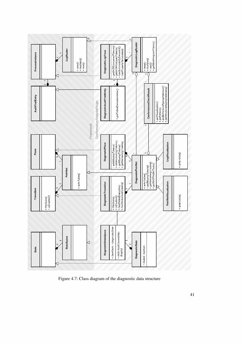
Figure 4.7: Class diagram of the diagnostic data structure

41

Log Replay Involving Invisible and Duplicate Tasks

functionality inherited from the framework while enhancing it with the diagnostic data collected.As an example the class DiagnosticTransition overrides isEnabled() inherited from theclass Transition to fire the shortest sequence of invisible tasks enabling the transition in ques-tion, if possible. To this end a partial exploration of the state space (i.e., the coverability graphprovided by the class DiagnosticStateSpace) based on the current marking of the net isnecessary. While firing a DiagnosticTransition the number of consumed and producedtokens is recorded, and if there are tokens missing or remaining after log replay this is recordedin the respective DiagnosticPlace.

For the visualization of diagnostic data the plug-in re-uses the Dot6 mechanism applied by theframework. Predefined methods like writeToDot() can be overridden to enhance the defaultimplementation of the PetriNet class by diagnostic information or to even change the view to,e.g., the log perspective.

4.3 Log Replay Involving Invisible and Duplicate Tasks

When performing such a non-blocking log replay involving invisible and duplicate tasks, situa-tions in the run of replay may be encountered where the state space of the process model needsto be partly explored. This is the case for the solution of two non-trivial problems described inthe following, namely whether a specific task can be enabled via firing a sequence of invisibletasks (see Section 4.3.1) and the decision for one task among duplicates (see Section 4.3.2).

To provide a link between the general problem solution and its implementation, Figures 4.8and 4.9 visualize the algorithms in a rather abstract way as a Petri net in FMC notation (whichwas chosen as it defines a standard way to model recursion7) while following the implementationstructure and indicating the names of the methods implemented.

4.3.1 Enabling a Task via Invisible Tasks

The first algorithm deals with the fact that invisible tasks are considered lazy, i.e., they mightfire in order to enable one of their succeeding visible tasks (recall that invisible tasks will neverbe fired directly in the flow of log replay since they do not have a log event associated). Thisimplies that in the case that the task currently replayed is not directly enabled, it must be checkedwhether it can be enabled by a sequence of invisible tasks before considering it having failed.The conflict between multiple enabling sequences is solved by choosing an arbitrary elementout of the set of shortest sequences. This aims at having minimal possible side effects on thecurrent marking of the net, e.g., not to unnecessarily fire an invisible task that is in conflictwith another task later to be replayed. Figure 4.8 shows the flow of the method isEnabled()

implemented in DiagnosticTransition, which has been overridden to replace the defaultbehavior of Transition in the following way.

Since a diagnostic transition can also be enabled “through” one or multiple invisible tasks,a list is created to capture this (potential) enabling sequence. If the transition is enabled

6Open source graph layout software used by the ProM framework for visualizing graph structures like, e.g., Petrinets or state spaces. Further information can be obtained from http://www.graphviz.org/.

7For the general recursion scheme and further examples refer to http://www.f-m-c.org/.

42

Figure 4.8: Recursive algorithm for transparently enabling a replayed task through a sequenceof invisible tasks (if possible)

43

Log Replay Involving Invisible and Duplicate Tasks

anyway, this sequence remains empty and the method returns true. Note that an empty list haslength 0 but is not nil (which could be seen as undefined). In the case of not being directlyenabled the state space is built from the current marking of the Petri net. To prevent nets thataccumulate tokens from producing an infinite state space (which could happen, e.g., buildingthe reachability graph of a Petri net) the coverability graph builder of the ProM framework hasbeen used for implementation. In a coverability graph a so-called ω-state denotes an extendedmarking, which subsumes all the different finite markings that result from token accumulationin an infinite marking [30, 33].

Then traceShortestPathOfInvisibleTasks()—the recursive program part—is called.Its input place is the entry point of the recursion, which means that initially called by the en-closing program part it can then be called several times from the recursive part itself. At thesame time a token is put in the stack place (S) for guiding the recursion handling. Stack placesare always input places for transitions that additionally have a return place (R) as input. All thestack places together constitute the return stack, which is used to store information about returnpositions. When the return place gets marked and more than one associated stack places have astack token the conflict is always solved in the same manner: the newest token on the stack mustbe consumed first. The newest token belongs to exactly one stack place and so the transitionwhere this stack place is an input place will fire.

Entering the recursive program part the idea is to trace each possible path of invisible tasks inthe state space until one of the following end-conditions is reached:

(a) If the current state was already visited during traversal, it means that the state space iscyclic and recursion stops to prevent an infinite loop.

(b) If a shorter sequence of invisible tasks enabling the transition in question than the onecurrently traced has already been found, it is not necessary to pursue this route any further.

Assuming that neither (a) nor (b) are fulfilled all possible paths from the current state in thestate space are considered and further traced as long as the next step is still an invisible task. Ifthis is the case the current state is marked as being visited already, the invisible task encounteredis appended to the currently pursued sequence, and passing the corresponding successor statetraceShortestPathOfInvisibleTasks() is called recursively. At the same time a tokenis put in the stack place8 to continue handling this path after the procedure returns. Since the timestamp9 of this token is more recent than the one of the token in the stack place of the enclosingprogram part, the conflict is always solved in favor of the transition in the recursive part. Onlyif there is no token left in this multi-token stack place, i.e., the recursion is completely handled,the procedure will return to getShortestSequenceOfInvisibleTasks().

On a logical level, there are two more end-conditions that can be reached evaluating all pos-sible future steps based on the current traversal state:

(c) If the transition to be replayed is encountered, a possible enabling sequence has beenfound and will be returned.

8Enlarged places such as this stack place can hold multiple tokens at the same time. The amount can be limited andannotated at the place while a double circle denotes an infinite capacity.

9Here a notion similar to Colored Petri Nets (CPN) [25] has been used, i.e., the possibility to assign a token differentvalues such as a time stamp.

44

(d) If no invisible task can be found, recursion aborts as the path cannot be followed anyfurther.

Following the flow of the algorithm to its end it must be kept in mind that the place holderfor the best sequence, referred to as the so far shortest, remains nil until the requestedtransition was encountered at least once while tracing those paths of invisible tasks in the statespace. If no possible sequence could be found, i.e., the checked diagnostic transition cannot beenabled via firing any invisible tasks either, the list will be set to nil and the method returnsfalse. However, in the case a possible path has been found, the gained sequence of invisibletasks is executed to transparently enable the diagnostic transition and the method returns true.

4.3.2 Choosing a Duplicate Task

The second algorithm deals with the fact that the mapping between model tasks and log events(see also Section 2.3) may result in duplicate tasks. During log replay this is a problem sinceencountering a log event being associated with multiple tasks in the model it is not alwaysclear which of the duplicates should be executed. The overall goal will be to replay a logcorrectly, if possible. Figure 4.9 shows the flow of the solution implemented by the methodchooseEnabledDuplicateTask(), which is called by replayTrace() in the case of find-ing more than one transition associated with the log event currently replayed.

At first, only those tasks being enabled10 by the current marking of the Petri net are selected.If there is none enabled the method returns immediately and the ConformanceChecker willfire an arbitrary task from the list of duplicates (since correct replay is not possible anyway).If there is exactly one task enabled it is returned and will be executed subsequently. This willoften be the case in scenarios where the same task is carried out in multiple contexts (such assetting a checkpoint at the begin and at the end of a the example process in Figure 3.1), i.e., themarking of the net clearly indicates which choice is best. However, if there are more candidatesenabled the remaining log events must be considered to determine the best choice. For thesepurposes, chooseBestCandidate() is called, making a copy of the current replay scenariofor each enabled duplicate and firing the transition belonging to that candidate (i.e., starting toplay over every case). Then the entry point for the recursive method tracking these scenarios,i.e., traceBestCandidate(), is reached and will not return until there is only one scenarioleft, which can then be reported to the initial caller in order to proceed with the actual log replay.

Entering the recursive program part at first the following end-condition is checked:

(a) If there are no log events left in the trace currently being replayed, one of the remainingcandidates is chosen arbitrarily and recursion is finished.

Assuming that (a) is not fulfilled the next log event is fetched from the trace and the numberof associated transitions is determined. If there is only one task associated to it, those scenariosare kept and updated where this task is enabled, i.e., where the next replay step can be executedsuccessfully as well. If there are multiple tasks associated, the best duplicate must also be chosen

10Note that in the context of this algorithm the possibility of invisible tasks indirectly enabling other transitions needsto be respected again (but without actually changing the marking of the replayed net). However, from now on itis abstracted from this issue.

45

Log Replay Involving Invisible and Duplicate Tasks

Figure 4.9: Recursive algorithm for choosing a duplicate task during log replay

46

for this case and for each scenario, realized by a recursive call to the very entry point of thewhole procedure. Note that the enclosing program part belonging to this recursive call, which isreplayTrace(), is not contained in the picture. Then, similarly, those scenarios are kept andupdated that were able to determine an enabled duplicate task for this anticipated next replaystep. The possibility for having a 0:1 mapping has been discarded since the log is—accordingto Section 2.3—assumed to be pre-processed, i.e., log events not associated to any task in themodel were removed during import.

Now, the number of remaining scenarios is checked and if there are more than one left re-cursion proceeds to check at least one step further. Otherwise one of the two following end-conditions is reached, stopping the recursion:

(b) If only one candidate remains, this one is returned as the best choice.

(c) If, after replaying this next log event, none of the scenarios is left, any of the previouslykept candidates is returned.

4.4 Assessment and Future Implementation Work

Regarding the algorithms presented in the last section, it is important to be aware of the factthat, e.g., choosing any duplicate task in the case of none of them being enabled in the firstplace, might render a log replay non-deterministic on a logical level. This does not mean thatanalyzing the same two files (containing the model and the log, respectively) might becomenon-deterministic, it will always yield identical results. However, this is not necessarily the caseas soon as the Petri net file is exchanged by another one, still defining the same Petri net (i.e.,on a logical level) but syntactically specifying the transitions in a different order. This leads toa differently ordered list held internally after import, which in the case of choosing any non-enabled duplicate task might then lead to firing another transition, possibly leaving more tokensin the net and thus affecting the metrics f and aB .

On this semantic level a fully deterministic log replay involving invisible and duplicate taskscannot be ensured by definition. But also guaranteeing equal values for the metrics calculatedwould dramatically increase complexity as the state space would need to be explored in a muchmore extensive way, comparing the amount of produced, consumed, missing, and remaining to-kens, and enabled transitions for every possible scenario. So clearly there is a trade-off betweenfull reproducibility according to Requirement 4 from Section 2.1 and performance, which can beexpected to decrease considerably and therefore hinder useful application while adding very lit-tle practical value (as this semantic non-determinism will only cause f and aB value deviationswhile analyzing poorly fitting logs in conjunction with models involving duplicate tasks).

However, if the log fits the model the conformance analysis plug-in is able to replay the logcorrectly, also while dealing with invisible and duplicate tasks. This is very important as anymismatch thus really indicates a conformance problem, which can then be quantified to assessits dimension and located to further analyze possible causes and corrective actions.

47

Assessment and Future Implementation Work

The performance of the log replay procedure as it is implemented in the conformance checkeris hard to appraise. It might vary a lot, depending on how many duplicate and invisible tasks areinvolved as in this case the state space needs to be partially explored. But even the fact that, e.g.,the state space of the model is built after each replay step for the current marking of the net todetermine the number of enabled transitions (for a transition potentially being enabled throughan invisible task), which is needed to calculate the metric aB , might cause problems in the casethat the state space is very large.

So it is intended to make the implementation more flexible by offering the choice for whichmetrics should actually be calculated. But in general the log replay approach is very promisingas for models not containing any invisible or duplicate tasks the complexity is proportional to thesize of the log (and does not have to deal with the issue of completeness). It would be importantto verify the presented techniques with respect to real business scenarios, e.g., in the form of acase study. Therefore, the improved appropriateness metrics should also be implemented in theconformance checker.

Regarding implementation of the improved behavioral appropriateness metric a′B one wouldfirst derive the SF and SB relations from the state space of the process model. This could be abottleneck as for it the state space of the model needs to be fully explored. Then, they would beverified with respect to the log. In fact, one could aim at the falsification of both counterpartsfor each pair of labels contained in Sm

F and SmB , making use of the fact that (x, y) ∈ SF iff

(x, y) /∈ AF ∧ (x, y) /∈ NF , or (x, y) ∈ SB iff (x, y) /∈ AB ∧ (x, y) /∈ NB , respectively. Thecost for this part of the analysis will increase proportionally with the size of the (aggregated)log.

It would be interesting to validate the presented metric with respect to some real businessprocesses as the global character of the approach on the one hand promises to incorporate free-choice constructs (i.e., control flow constraints that cannot be recognized from local dependen-cies), but on the other hand it also seems as if non-short loops dilute the footprints of theirenclosed tasks in such a way that the Never relations disappear.

In general, the idea to verify certain properties for a set of log traces is related to the LTLchecker [10], which has been implemented as a plug-in for the ProM framework. Linear Tem-poral Logic (LTL) is a field of mathematical logic that is able to talk about the future of paths.The LTL checker is able to verify a given LTL expression with respect to a given workflow log.

As far as the implementation of the improved structural appropriateness metric a′S is con-cerned, alternative ways to determine the set of redundant invisible tasks IR should be examinedas the current definition requires a complete exploration of the (modified) state space for everyinvisible task in the model. For determining the set of alternative duplicate tasks DA one wouldalso need to fully explore the transition system corresponding to the process model once (which,as discussed, could cause problems for a very big state space). However, if it is possible then itcan be realized together with the derivation of the relations Sm

F and SmB for the metric a′B .

48

5 Related Work

Regarding its purpose conformance testing as presented in this paper is closely related to thework of Cook et al. [12, 11] who have introduced the concept of process validation. They pro-pose a technique comparing the event stream coming from the process model with the eventstream from the execution log (cf. Section 2) based on two different string distance metrics. Toface the problem of time-complexity while exploring the state space of the model they investi-gate (and reject) several techniques from domains like compiler research and regular-expressionmatching. In the end an incremental, data-driven state-space search is suggested, using heuris-tics to reduce the cost. An interesting point is that they include the possibility to assign weightsin order to differentiate the relative importance of specific types of events. In [11] the resultsare extended to include time aspects. The notion of conformance has also been discussed in thecontext of business alignment [1], security [4], and genetic mining [28] (all proposing some kindof replay).

However, in each of the papers mentioned only fitness is considered and appropriateness ismostly ignored.

Conformance testing assumes the presence of a given descriptive or prescriptive processmodel, and therefore has a different starting point, but nevertheless it is closely related to processmining [7, 6], which aims at the discovery of a process model based on some event log. In thedesire to derive a “good” model for the behavior observed in the execution log, shared notionsof fitness, behavioral appropriateness and structural appropriateness can be recognized.

In [20] the process mining problem is faced with the aim of deriving a model which is ascompliant as possible with the log data, accounting for fitness (called completeness) and alsobehavioral appropriateness (called soundness). Starting with a disjunctive workflow schemacontaining all the traces from the log (cf. Figure 3.4) they try to incrementally cluster thesetraces until a given lower bound for the number of schemata contained is reached, which, in fact,corresponds to some notion of structural appropriateness as well.

Another example is the process mining approach presented in [34], which is aiming at thediscovery of a WF-net that (i) potentially generates all event sequences appearing in the execu-tion log (i.e., fitness), (ii) generates as few event sequences not contained in the execution log aspossible (i.e., behavioral appropriateness), and (iii) captures concurrent behavior and (iv) is assimple and compact as possible (i.e., structural appropriateness).

Moreover, techniques such as considering some form of causal relation can be borrowed fromthe process mining research, just as insights gained into concepts like correctness, completeness,and noise are also relevant in the context of conformance testing.

Both process mining and conformance testing can be seen in the broader context of Busi-ness (Process) Intelligence (BPI) and Business Activity Monitoring (BAM). Tools, as describedin [21, 29, 22], however, often focus on performance measurements rather than monitoring

49

Related Work

(un)desirable behavior.

50

6 Conclusion

From the coexistence of explicit process models and event logs originates the interesting ques-tion “Do the model and the log conform to each other?”. This question is highly relevant as theirdiversion is expected, yet indicates a clearly undesirable inconsistent state.

This paper proposes an incremental approach to check the conformance of a process modeland an event log. At first, the fitness between the log and the model needs to be ensured (i.e.,“Does the observed process comply with the control flow specified by the process model?”). Atsecond, the appropriateness of the model can be analyzed with respect to the log (i.e., “Does themodel describe the observed process in a suitable way?”). During this second phase two aspectsof appropriateness are considered, evaluating structural properties of the process model on theone hand (“Is the behavior specified by the model represented in a structurally suitable way?”)and behavioral properties on the other (“Does the model specify the behavior of the observedprocess in a sufficiently specific way?”).

One metric (f ) has been defined to address fitness and two metrics each approach structuralappropriateness (aS and a′S) and behavioral appropriateness (aB and a′B). Together they allowfor the quantification of conformance, whereas fitness should be ensured before appropriatenessis analyzed. However, since in real life business scenarios a fitness of 100% is unlikely, it wouldbe interesting to investigate until which degree of fitness the behavioral appropriateness anal-ysis can still produce useful results, or to even explicitly develop a behavioral appropriatenesstechnique that is able to deal with noise. Furthermore, as shown in this paper behavioral ap-propriateness requires some notion of completeness by definition. Structural appropriateness, incontrast, can even be evaluated independently of the logged data at all as only the suitability ofthe model in representing the specified behavior is appraised. To ensure the usefulness of themetrics defined three requirements were formulated, calling for their (1) validity, (2) stability,and (3) reproducibility. A violation of the second requirement has led to the development of thetwo alternative appropriateness metrics a′S and a′B , which—in contrast to their counterparts aS

and aB—are able to measure only one dimension of appropriateness, independently of the other.Besides the quantification of fitness and appropriateness, it is crucial to assist the analyst in

finding the location of a conformance problem. It has been shown that the approaches presentedfor the formation of f , a′S , and a′B are able to locate the respective problem areas in the modelor the log.

So the presented techniques constitute a powerful means to indicate a conformance problemand to estimate its dimension, while providing the user with some visual feedback pinpointingthose parts that should be revised.

Future work will aim at the implementation of the alternative appropriateness approaches a′Band a′S in the first place, to enable the application of all the presented techniques in real businessscenarios, and for the appraisal of the metrics themselves (with respect to performance andeffectiveness). To really support the incremental character of the presented approach it would

51

Conclusion

be nice if one could—following the suggestions of the conformance analysis tool—simulateadjustments in both the model and the log in order to, e.g., proceed with the analysis of anotherconformance aspect.

Naturally, additional information about both the application context and the technology usedcan be exploited to extend and/or customize the conformance analysis techniques presented inthis paper. As an example, for monitoring a business process that follows a carefully designed,prescriptive process model, it could be desirable to carry out the log replay from a model-basedperspective (i.e., following the track of the model instead of inserting tokens where they areneeded). In doing so one could punish a sequence of missing activities to a greater extent thana single missing activity (which is not the case for the log replay analysis as presented), but thisis expected to be a very complex approach as it results in a far more extensive exploration of themodel’s state space. Moreover, knowing the logging facilities of a workflow product in detailenables a more in-depth evaluation of low level log events such as those related to the life cycleof a task (i.e., schedule, assign, start, suspend, ...), and the availability of time stamps makes theverification of time constraints, such as meeting a deadline, possible.

Finally, the incorporation of other perspectives is expected to enrich the conclusions derivedfrom conformance analysis. For example, the evaluation of the organizational perspective (i.e.,groups and roles) might provide insight into diverging processes in different departments of acompany.

52

References

[1] W.M.P. van der Aalst. Business Alignment: Using Process Mining as a Tool for DeltaAnalysis. In J. Grundspenkis and M. Kirikova, editors, Proceedings of the 5th Workshop onBusiness Process Modeling, Development and Support (BPMDS’04), volume 2 of Caise’04Workshops, pages 138–145. Riga Technical University, Latvia, 2004.

[2] W.M.P. van der Aalst and K.M. van Hee. Workflow Management: Models, Methods, andSystems. MIT press, Cambridge, MA, 2002.

[3] W.M.P. van der Aalst, A.H.M. ter Hofstede, B. Kiepuszewski, and A.P. Barros. WorkflowPatterns. Distributed and Parallel Databases, 14(1):5–51, 2003.

[4] W.M.P. van der Aalst and A.K.A. de Medeiros. Process Mining and Security: DetectingAnomalous Process Executions and Checking Process Conformance. In N. Busi, R. Gor-rieri, and F. Martinelli, editors, Second International Workshop on Security Issues withPetri Nets and other Computational Models (WISP 2004), pages 69–84. STAR, ServizioTipografico Area della Ricerca, CNR Pisa, Italy, 2004.

[5] W.M.P. van der Aalst and M. Song. Mining Social Networks: Uncovering InteractionPatterns in Business Processes. In J. Desel, B. Pernici, and M. Weske, editors, InternationalConference on Business Process Management (BPM 2004), volume 3080 of Lecture Notesin Computer Science, pages 244–260. Springer-Verlag, Berlin, 2004.

[6] W.M.P. van der Aalst, B.F. van Dongen, J. Herbst, L. Maruster, G. Schimm, and A.J.M.M.Weijters. Workflow Mining: A Survey of Issues and Approaches. Data and KnowledgeEngineering, 47(2):237–267, 2003.

[7] W.M.P. van der Aalst and A.J.M.M. Weijters, editors. Process Mining, Special Issue ofComputers in Industry, Volume 53, Number 3. Elsevier Science Publishers, Amsterdam,2004.

[8] W.M.P. van der Aalst, A.J.M.M. Weijters, and L. Maruster. Workflow Mining: DiscoveringProcess Models from Event Logs. IEEE Transactions on Knowledge and Data Engineer-ing, 16(9):1128–1142, 2004.

[9] Pallas Athena. Flower User Manual. Pallas Athena BV, Apeldoorn, The Netherlands,2002.

[10] H. de Beer. The LTL Checker Plugins: A Reference Manual. Eindhoven University ofTechnology, Eindhoven, 2004.

53

References

[11] J.E. Cook, C. He, and C. Ma. Measuring Behavioral Correspondence to a Timed Concur-rent Model. In Proceedings of the 2001 International Conference on Software Mainenance,pages 332–341, 2001.

[12] J.E. Cook and A.L. Wolf. Software Process Validation: Quantitatively Measuring theCorrespondence of a Process to a Model. ACM Transactions on Software Engineering andMethodology, 8(2):147–176, 1999.

[13] G. Cugola, E. Di Nitto, A. Fuggetta, and C. Ghezzi. A Framwork for Formalizing In-consistencies and Deviations in Human-centered Systems. ACM Transactions on SoftwareEngineering and Methodology, 5(3):191–230, 1996.

[14] J. Desel and J. Esparza. Free Choice Petri Nets, volume 40 of Cambridge Tracts in Theo-retical Computer Science. Cambridge University Press, Cambridge, UK, 1995.

[15] J. Desel, W. Reisig, and G. Rozenberg, editors. Lectures on Concurrency and Petri Nets,volume 3098 of Lecture Notes in Computer Science. Springer-Verlag, Berlin, 2004.

[16] B.F. van Dongen and W.M.P. van der Aalst. Multi-Phase Process Mining: Building In-stance Graphs. In P. Atzeni, W. Chu, H. Lu, S. Zhou, and T.W. Ling, editors, InternationalConference on Conceptual Modeling (ER 2004), volume 3288 of Lecture Notes in Com-puter Science, pages 362–376. Springer-Verlag, Berlin, 2004.

[17] B.F. van Dongen, W.M.P. van der Aalst, and H.M.W. Verbeek. Verification of EPCs: Us-ing Reduction Rules and Petri Nets for Systems Engineering: A Guide to Modeling, Ver-ification, and Applications. In 17th International Conference, CAiSE 2005, Porto, pages372–386. Springer-Verlag, Berlin, 2005.

[18] N.E. Fenton and S.L. Pfleeger. Software Metrics - A Rigorous & Practical Approach (2ndEdition). PWS Publishing Company, Boston, 1998.

[19] M. van Giessel. Process Mining in SAP R/3. Master’s thesis, Eindhoven University ofTechnology, Eindhoven, 2004.

[20] G. Greco, A. Guzzo, L. Pontieri, and D. Sacca. Mining Expressive Process Models byClustering Workflow Traces. Proc of Advances in Kowledge Discovery and Data Mining,8th Pacific-Asia Conference (PAKDD 2004), pages 52–62, 2004.

[21] D. Grigori, F. Casati, M. Castellanos, U. Dayal, M. Sayal, and M.C. Shan. Business processintelligence. Computers in Industry, 53(3):321–343, 2004.

[22] IDS Scheer. ARIS Process Performance Manager (ARIS PPM): Measure, Analyze andOptimize Your Business Process Performance (whitepaper). IDS Scheer, Saarbruecken,Gemany, http://www.ids-scheer.com, 2002.

[23] F. Keller, P. Tabeling, R. Apfelbacher, B. Grone, A. Knopfel, R. Kugel, and O. Schmidt.Improving Knowledge Transfer at the Architectural Level: Concepts and Notations. InProceedings of The 2002 International Conference on Software Engineering Research andPractice, Las Vegas), 2002.

54

References

[24] G. Keller and T. Teufel. SAP R/3 Process Oriented Implementation. Addison-Wesley,Reading MA, 1998.

[25] L.M. Kristensen, S. Christensen, and K. Jensen. The Practitioner’s Guide to Coloured PetriNets. International Journal on Software Tools for Technology Transfer, 2(2):98–132, 1998.

[26] J.B. Kruskal. An Overview of Sequence Comparison. Time Warps, String Edits,and Macromolecules: The Theory and Practice of Sequence Comparison, pages 1–44,Addison-Wesley, Reading MA, 1983.

[27] P. Liggesmeyer. Software-Qualitat – Testen, Analysieren und Verifizieren von Software.Spektrum Akademischer Verlag, Heidelberg, Berlin, 2002.

[28] A.K.A. de Medeiros, A.J.M.M. Weijters, and W.M.P. van der Aalst. Using Genetic Algo-rithms to Mine Process Models: Representation, Operators and Results. Technical report,BETA Working Paper Series, WP 124, Eindhoven University of Technology, Eindhoven,2004.

[29] M. zur Muhlen and M. Rosemann. Workflow-based Process Monitoring and Controlling -Technical and Organizational Issues. In R. Sprague, editor, Proceedings of the 33rd HawaiiInternational Conference on System Science (HICSS-33), pages 1–10. IEEE Computer So-ciety Press, Los Alamitos, California, 2000.

[30] T. Murata. Petri Nets: Properties, Analysis and Applications. Proceedings of the IEEE,77(4):541–580, April 1989.

[31] Mike O’Docherty. Object-Oriented Analysis and Design: Understanding System Develop-ment with UML 2.0. John Wiley and Sons, 2005.

[32] A.W. Scheer. ARIS: Business Process Modelling. Springer-Verlag, Berlin, 2000.

[33] H.M.W. Verbeek. Verification of WF-nets. PhD thesis, Eindhoven University of Technol-ogy, Eindhoven, The Netherlands, 2004.

[34] A.J.M.M. Weijters and W.M.P. van der Aalst. Rediscovering Workflow Models fromEvent-Based Data. In Proceedings of the Third International NAISO Symposium onEngineering of Intelligent Systems (EIS 2002), pages 65–65. NAISO Academic Press,Sliedrecht, The Netherlands, 2002. Full paper on CD-rom proceedings.

[35] H. Zuse. Software Complexity – Measures and Methods, volume 44 of Programming Com-plex Systems. Walter de Gruyter & Co., Berlin, New York, 1991.

55