Embed Size (px)
Citation preview
Conjugate gradients, sparse matrix-vector multiplication,
graphs, and meshes
Thanks to Aydin Buluc, Umit Catalyurek, Alan Edelman, and Kathy Yelick
for some of these slides.
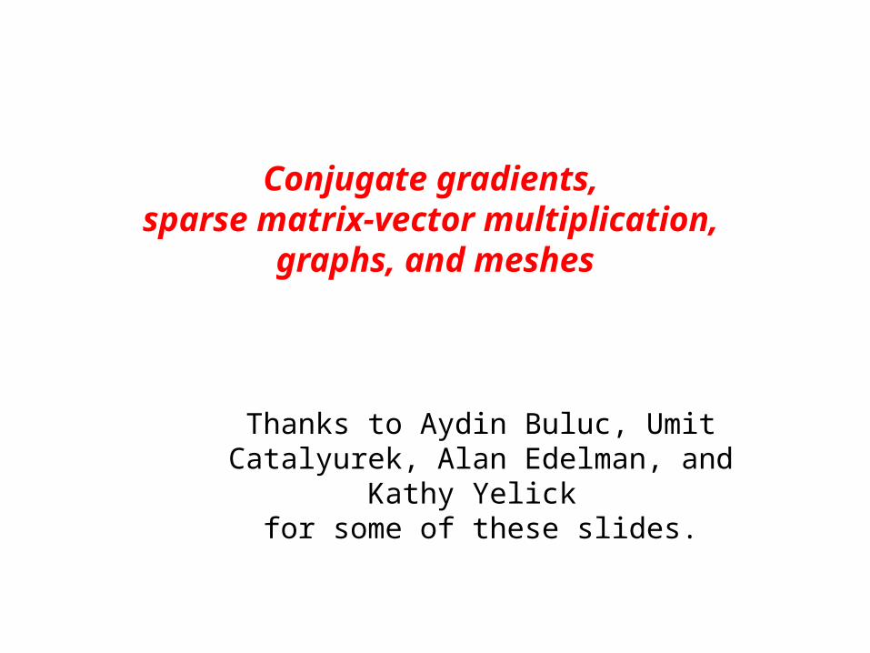
The middleware of scientific computing
Computers
Continuousphysical modeling
Linear algebra Ax = b
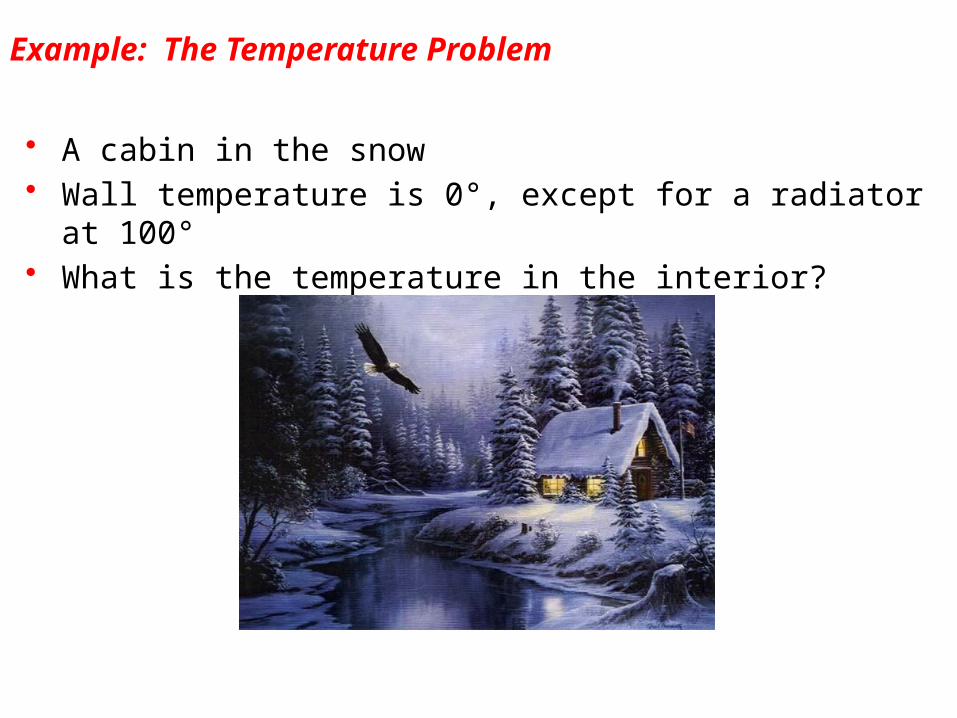
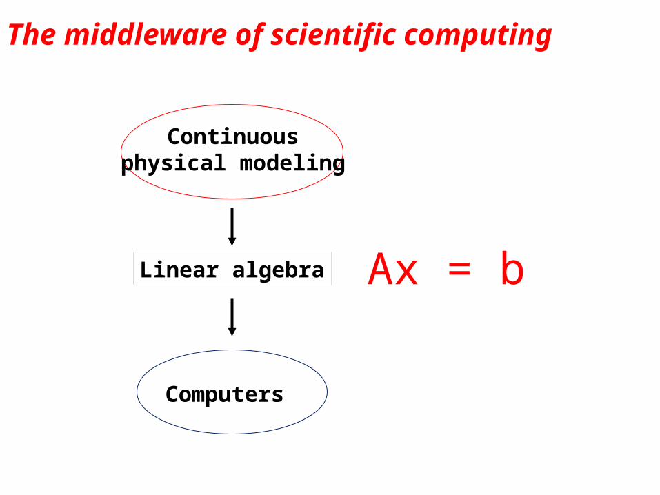
Example: The Temperature Problem
• A cabin in the snow• Wall temperature is 0°, except for a radiator at 100°• What is the temperature in the interior?
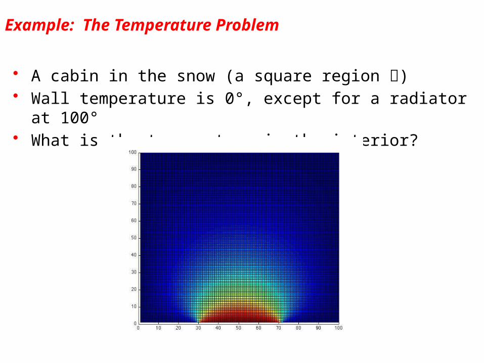
Example: The Temperature Problem
• A cabin in the snow (a square region )• Wall temperature is 0°, except for a radiator at 100°• What is the temperature in the interior?
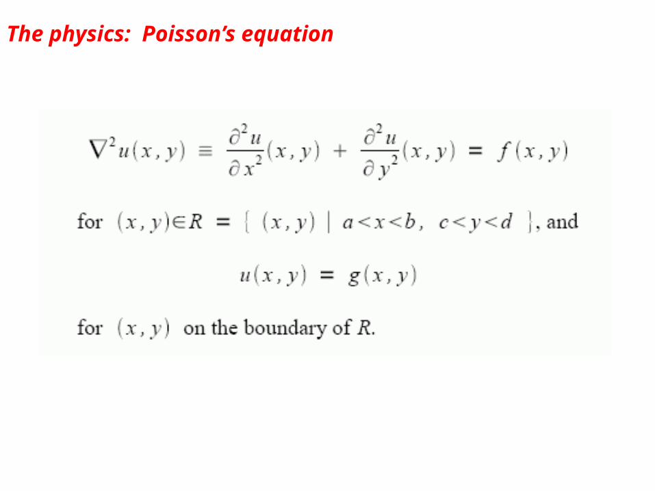
The physics: Poisson’s equation
6.43
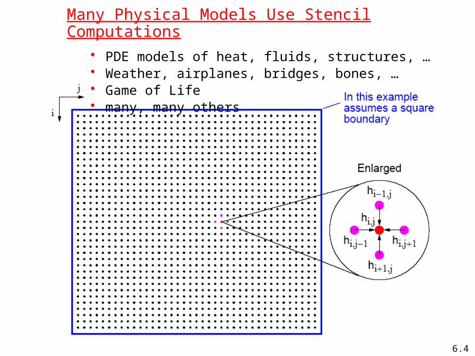
Many Physical Models Use Stencil Computations
• PDE models of heat, fluids, structures, …• Weather, airplanes, bridges, bones, …• Game of Life• many, many others
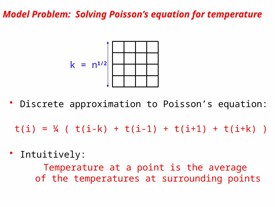
Model Problem: Solving Poisson’s equation for temperature
• Discrete approximation to Poisson’s equation:
t(i) = ¼ ( t(i-k) + t(i-1) + t(i+1) + t(i+k) )
• Intuitively:
Temperature at a point is the average of the temperatures at surrounding points
k = n1/2
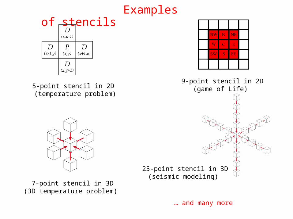
Examples of stencils
5-point stencil in 2D (temperature problem)
9-point stencil in 2D(game of Life)
7-point stencil in 3D(3D temperature problem)
25-point stencil in 3D(seismic modeling)
… and many more
9
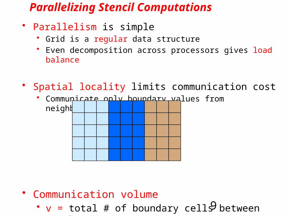
Parallelizing Stencil Computations
• Parallelism is simple• Grid is a regular data structure• Even decomposition across processors gives load balance
• Spatial locality limits communication cost• Communicate only boundary values from neighboring patches
• Communication volume • v = total # of boundary cells between patches
10
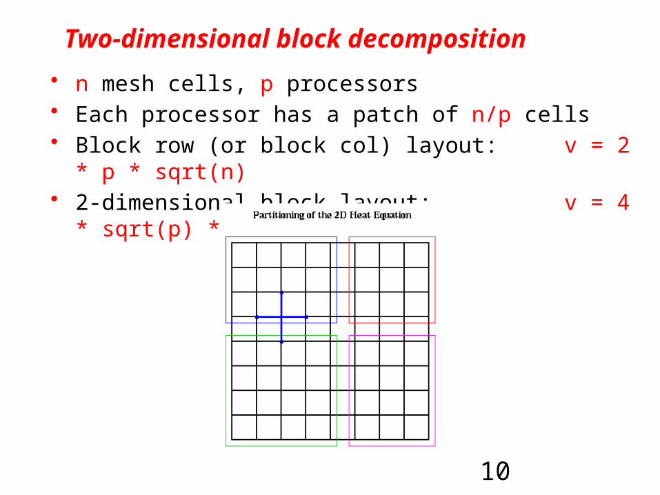
Two-dimensional block decomposition
• n mesh cells, p processors• Each processor has a patch of n/p cells• Block row (or block col) layout: v = 2 * p * sqrt(n)• 2-dimensional block layout: v = 4 * sqrt(p) * sqrt(n)
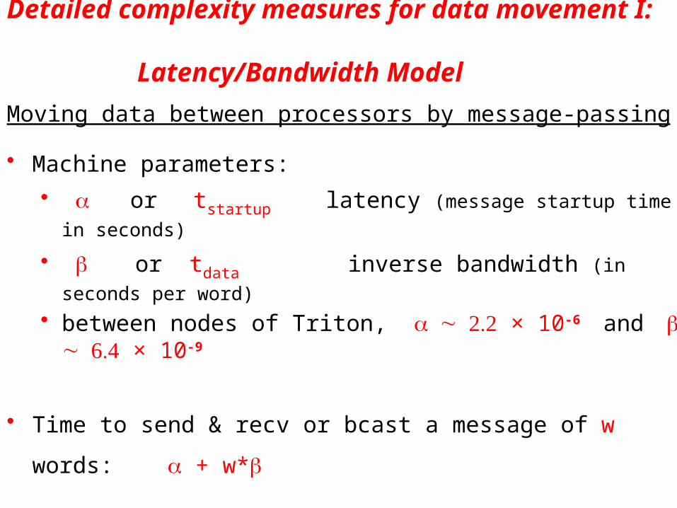
Detailed complexity measures for data movement I: Latency/Bandwidth Model
Moving data between processors by message-passing
• Machine parameters:
• a or tstartup latency (message startup time in seconds)
• b or tdata inverse bandwidth (in seconds per word)
• between nodes of Triton, ~ 2.2a × 10-6 and ~ 6.4b × 10-9
• Time to send & recv or bcast a message of w words: a + w*b
• tcomm total commmunication time
• tcomp total computation time
• Total parallel time: tp = tcomp + tcomm
12
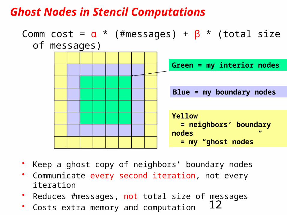
Ghost Nodes in Stencil Computations
Comm cost = α * (#messages) + β * (total size of messages)
• Keep a ghost copy of neighbors’ boundary nodes• Communicate every second iteration, not every iteration• Reduces #messages, not total size of messages• Costs extra memory and computation• Can also use more than one layer of ghost nodes
Green = my interior nodes
Yellow = neighbors’ boundary nodes = my “ghost nodes”
Blue = my boundary nodes
13
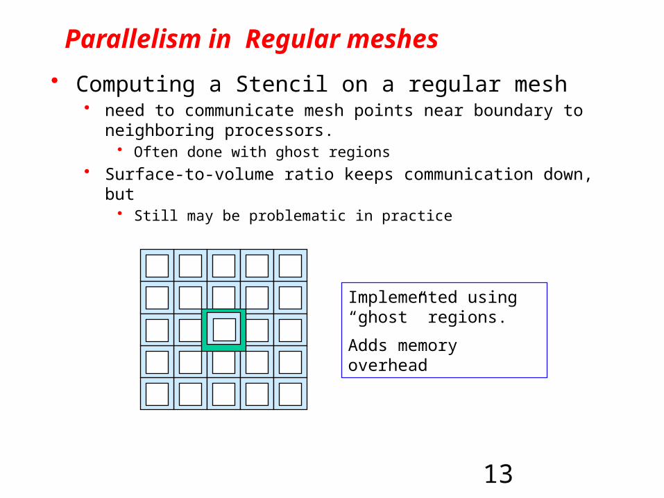
Parallelism in Regular meshes
• Computing a Stencil on a regular mesh• need to communicate mesh points near boundary to neighboring
processors.• Often done with ghost regions
• Surface-to-volume ratio keeps communication down, but• Still may be problematic in practice
Implemented using “ghost” regions.
Adds memory overhead

Model Problem: Solving Poisson’s equation for temperature
• Discrete approximation to Poisson’s equation:
t(i) = ¼ ( t(i-k) + t(i-1) + t(i+1) + t(i+k) )
• Intuitively:
Temperature at a point is the average of the temperatures at surrounding points
k = n1/2
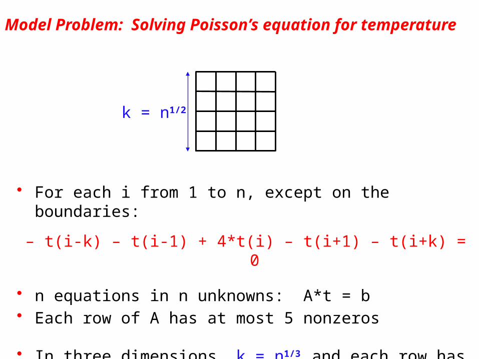
Model Problem: Solving Poisson’s equation for temperature
• For each i from 1 to n, except on the boundaries:
– t(i-k) – t(i-1) + 4*t(i) – t(i+1) – t(i+k) = 0
• n equations in n unknowns: A*t = b• Each row of A has at most 5 nonzeros
• In three dimensions, k = n1/3 and each row has at most 7 nzs
k = n1/2
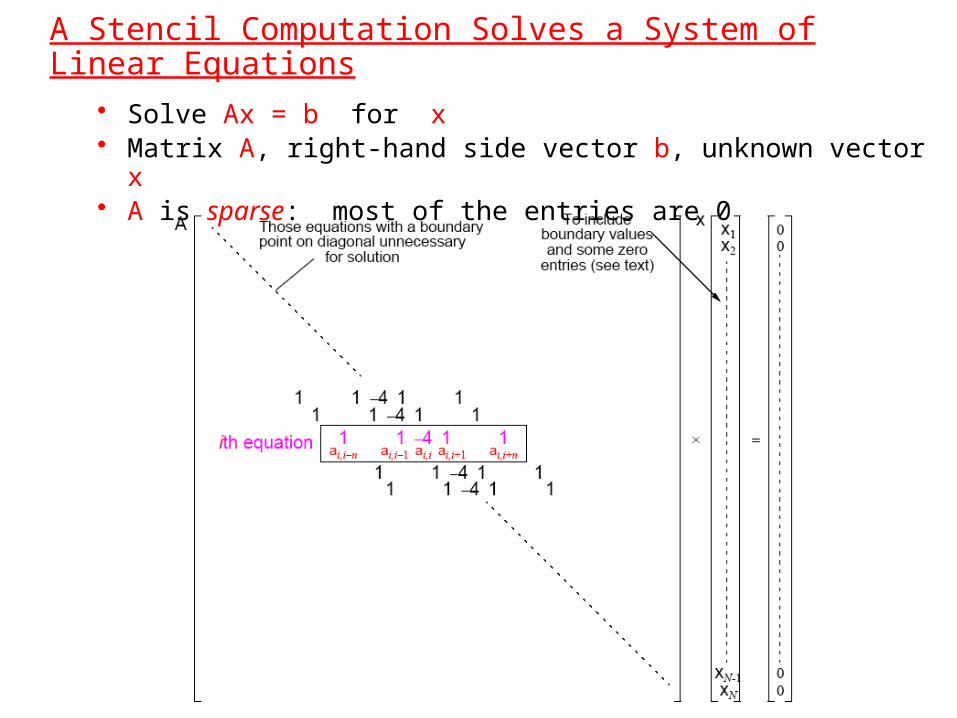
A Stencil Computation Solves a System of Linear Equations
• Solve Ax = b for x• Matrix A, right-hand side vector b, unknown vector x• A is sparse: most of the entries are 0
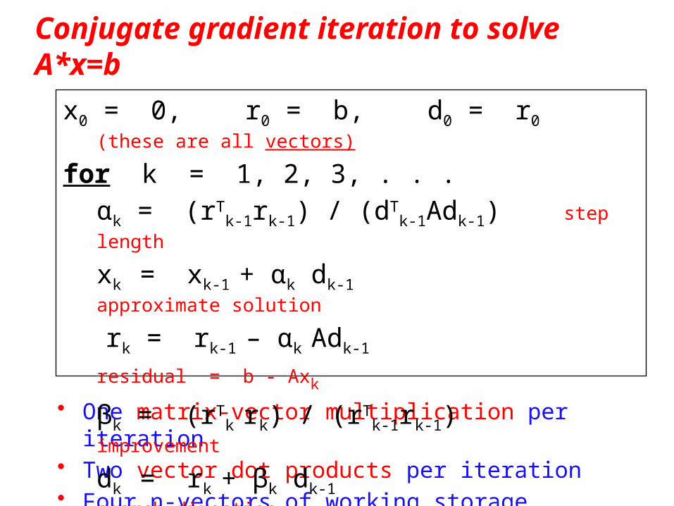
Conjugate gradient iteration to solve A*x=b
• One matrix-vector multiplication per iteration• Two vector dot products per iteration• Four n-vectors of working storage
x0 = 0, r0 = b, d0 = r0 (these are all vectors)
for k = 1, 2, 3, . . .
αk = (rTk-1rk-1) / (dT
k-1Adk-1) step length
xk = xk-1 + αk dk-1 approximate solution
rk = rk-1 – αk Adk-1 residual = b - Axk
βk = (rTk rk) / (rT
k-1rk-1) improvement
dk = rk + βk dk-1 search direction

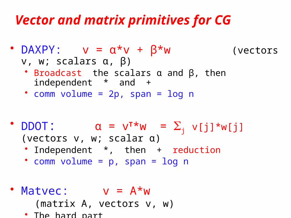
Vector and matrix primitives for CG
• DAXPY: v = α*v + β*w (vectors v, w; scalars α, β)• Broadcast the scalars α and β, then independent * and +• comm volume = 2p, span = log n
• DDOT: α = vT*w = Sj v[j]*w[j] (vectors v, w; scalar α)• Independent *, then + reduction• comm volume = p, span = log n
• Matvec: v = A*w (matrix A, vectors v, w)• The hard part• But all you need is a subroutine to compute v from w• Sometimes you don’t need to store A (e.g. temperature problem)• Usually you do need to store A, but it’s sparse ...
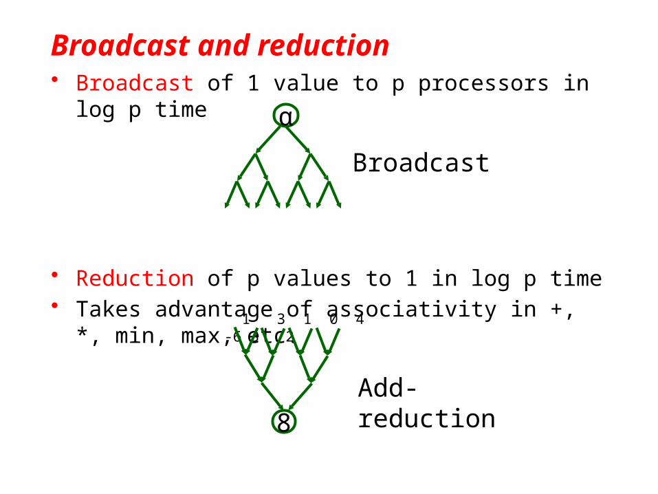
Broadcast and reduction• Broadcast of 1 value to p processors in log p time
• Reduction of p values to 1 in log p time• Takes advantage of associativity in +, *, min, max, etc.
α
8
1 3 1 0 4 -6 3 2
Add-reduction
Broadcast

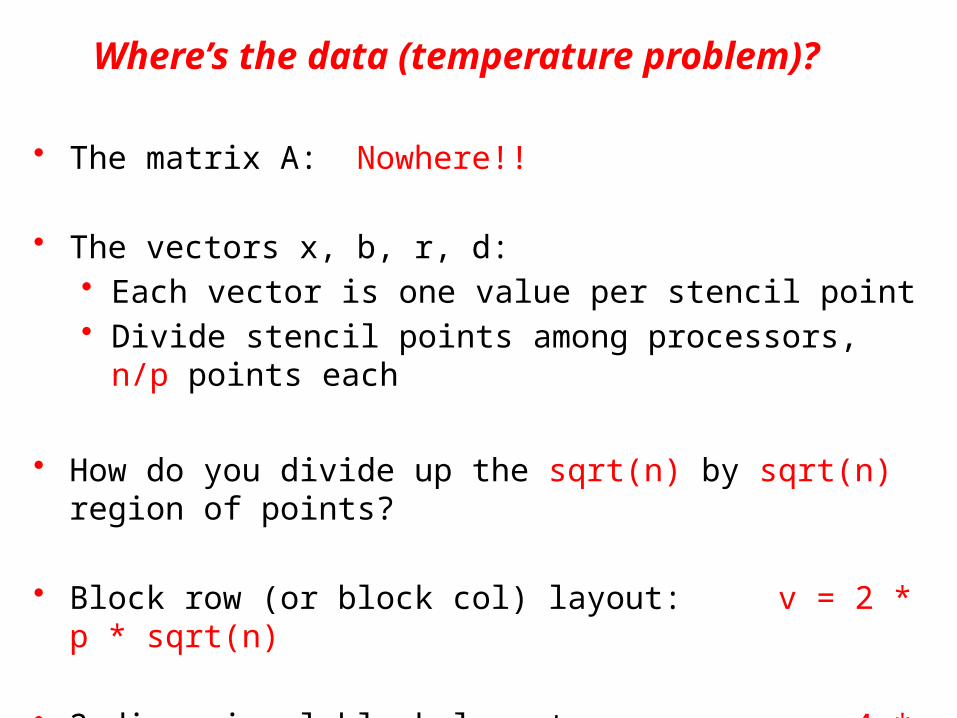
Where’s the data (temperature problem)?
• The matrix A: Nowhere!!
• The vectors x, b, r, d:• Each vector is one value per stencil point• Divide stencil points among processors, n/p points each
• How do you divide up the sqrt(n) by sqrt(n) region of points?
• Block row (or block col) layout: v = 2 * p * sqrt(n)
• 2-dimensional block layout: v = 4 * sqrt(p) * sqrt(n)
6.43
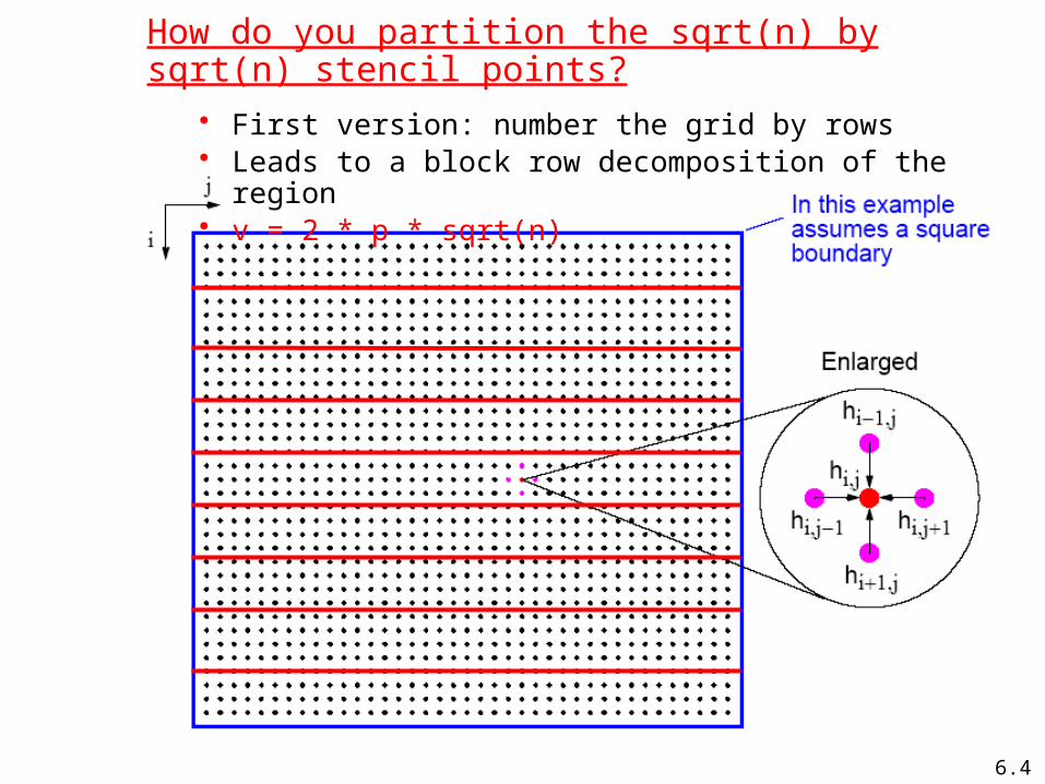
How do you partition the sqrt(n) by sqrt(n) stencil points?
• First version: number the grid by rows• Leads to a block row decomposition of the region• v = 2 * p * sqrt(n)
6.43
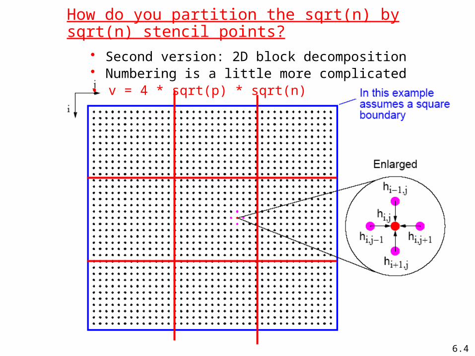
How do you partition the sqrt(n) by sqrt(n) stencil points?
• Second version: 2D block decomposition• Numbering is a little more complicated• v = 4 * sqrt(p) * sqrt(n)
Where’s the data (temperature problem)?
• The matrix A: Nowhere!!
• The vectors x, b, r, d:• Each vector is one value per stencil point• Divide stencil points among processors, n/p points each
• How do you divide up the sqrt(n) by sqrt(n) region of points?
• Block row (or block col) layout: v = 2 * p * sqrt(n)
• 2-dimensional block layout: v = 4 * sqrt(p) * sqrt(n)
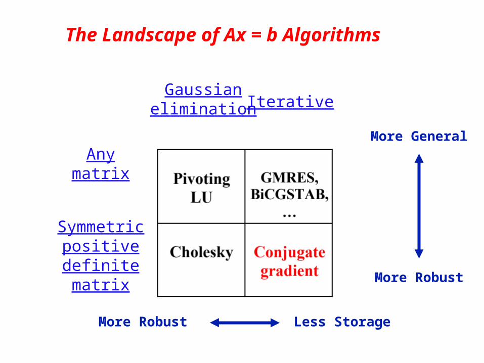
The Landscape of Ax = b Algorithms
Gaussianelimination Iterative
Anymatrix
Symmetricpositivedefinitematrix
More Robust Less Storage
More Robust
More General
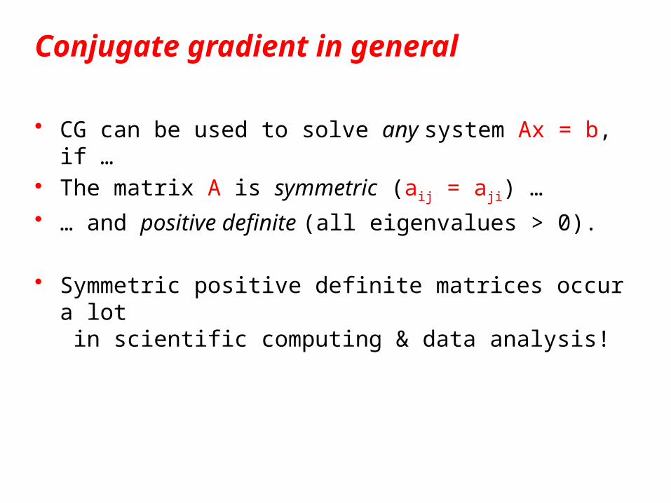
Conjugate gradient in general
• CG can be used to solve any system Ax = b, if …
Conjugate gradient in general
• CG can be used to solve any system Ax = b, if …• The matrix A is symmetric (aij = aji) …
• … and positive definite (all eigenvalues > 0).
Conjugate gradient in general
• CG can be used to solve any system Ax = b, if …• The matrix A is symmetric (aij = aji) …
• … and positive definite (all eigenvalues > 0).
• Symmetric positive definite matrices occur a lot in scientific computing & data analysis!

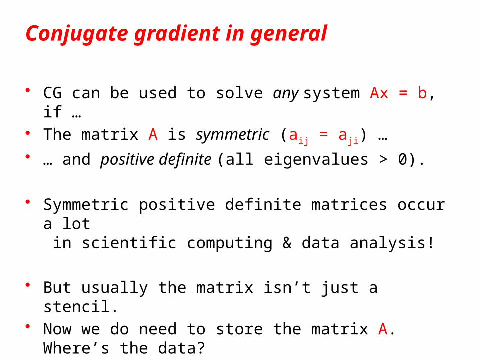
Conjugate gradient in general
• CG can be used to solve any system Ax = b, if …• The matrix A is symmetric (aij = aji) …
• … and positive definite (all eigenvalues > 0).
• Symmetric positive definite matrices occur a lot in scientific computing & data analysis!
• But usually the matrix isn’t just a stencil.• Now we do need to store the matrix A. Where’s the data?
• The key is to use graph data structures and algorithms.
Vector and matrix primitives for CG
• DAXPY: v = α*v + β*w (vectors v, w; scalars α, β)• Broadcast the scalars α and β, then independent * and +• comm volume = 2p, span = log n
• DDOT: α = vT*w = Sj v[j]*w[j] (vectors v, w; scalar α)• Independent *, then + reduction• comm volume = p, span = log n
• Matvec: v = A*w (matrix A, vectors v, w)• The hard part• But all you need is a subroutine to compute v from w• Sometimes you don’t need to store A (e.g. temperature problem)• Usually you do need to store A, but it’s sparse ...
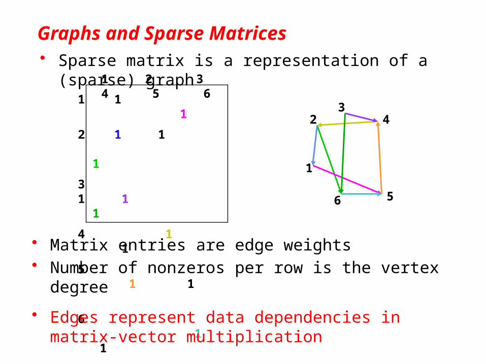
Graphs and Sparse Matrices
1 1 1
2 1 1 1
3 1 1 1
4 1 1
5 1 1
6 1 1
1 2 3 4 5 6
3
6
2
1
5
4
• Sparse matrix is a representation of a (sparse) graph
• Matrix entries are edge weights• Number of nonzeros per row is the vertex degree
• Edges represent data dependencies in matrix-vector multiplication
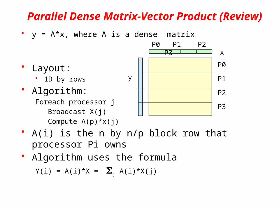
Parallel Dense Matrix-Vector Product (Review)
• y = A*x, where A is a dense matrix
• Layout: • 1D by rows
• Algorithm:Foreach processor j
Broadcast X(j)
Compute A(p)*x(j)
• A(i) is the n by n/p block row that processor Pi owns• Algorithm uses the formula
Y(i) = A(i)*X = Sj A(i)*X(j)
x
y
P0
P1
P2
P3
P0 P1 P2 P3
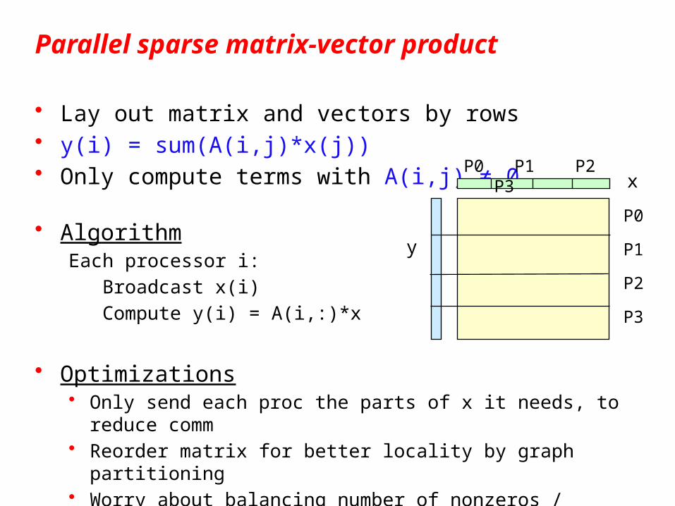
• Lay out matrix and vectors by rows• y(i) = sum(A(i,j)*x(j))• Only compute terms with A(i,j) ≠ 0
• AlgorithmEach processor i:
Broadcast x(i)
Compute y(i) = A(i,:)*x
• Optimizations• Only send each proc the parts of x it needs, to reduce comm • Reorder matrix for better locality by graph partitioning• Worry about balancing number of nonzeros / processor,
if rows have very different nonzero counts
x
y
P0
P1
P2
P3
P0 P1 P2 P3
Parallel sparse matrix-vector product
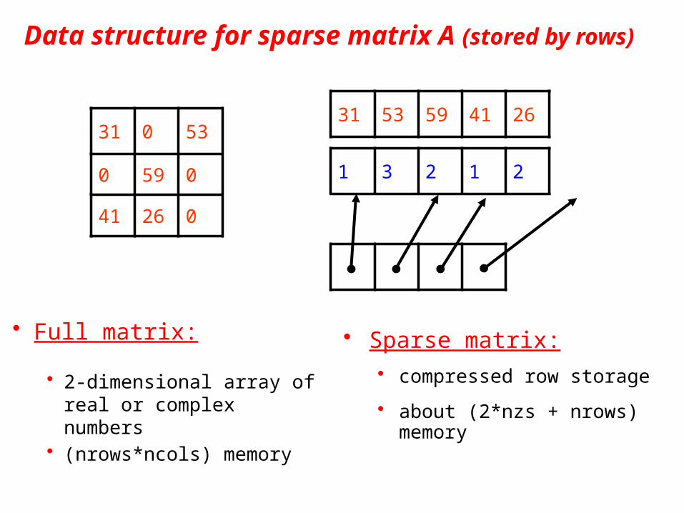
Data structure for sparse matrix A (stored by rows)
• Full matrix:
• 2-dimensional array of real or complex numbers
• (nrows*ncols) memory
31 0 53
0 59 0
41 26 0
31 53 59 41 26
1 3 2 1 2
• Sparse matrix:
• compressed row storage
• about (2*nzs + nrows) memory
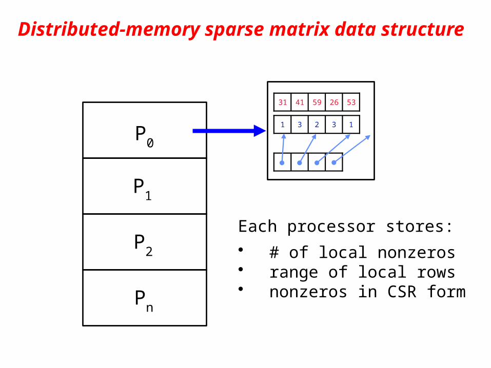
P0
P1
P2
Pn
5941 532631
23 131
Each processor stores:
• # of local nonzeros• range of local rows• nonzeros in CSR form
Distributed-memory sparse matrix data structure
36
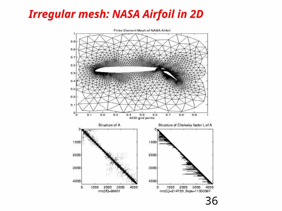
Irregular mesh: NASA Airfoil in 2D
37
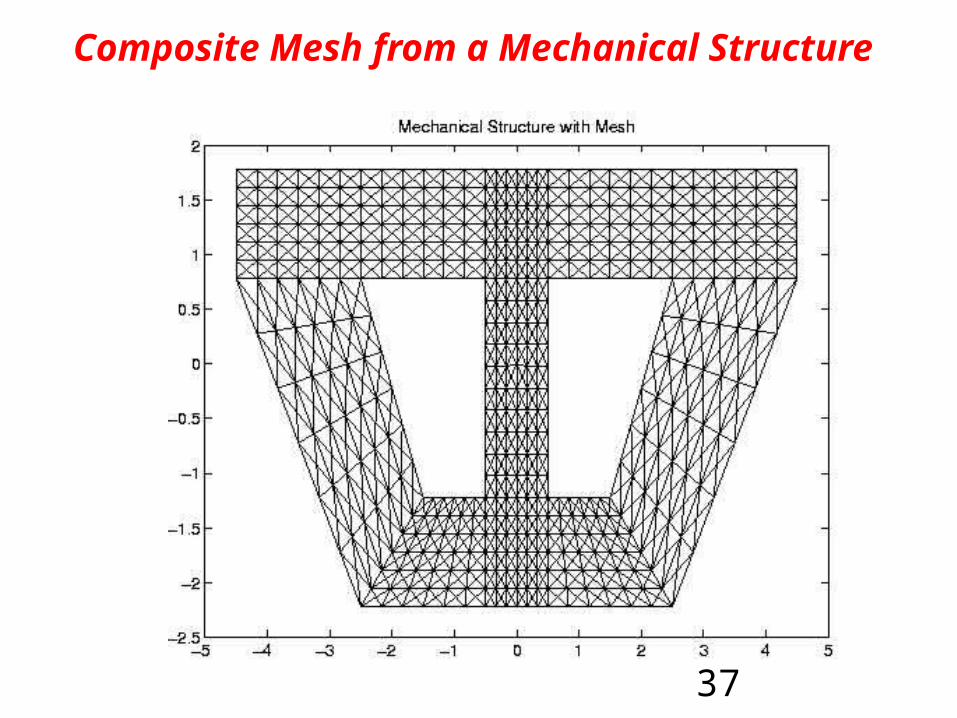
Composite Mesh from a Mechanical Structure
38
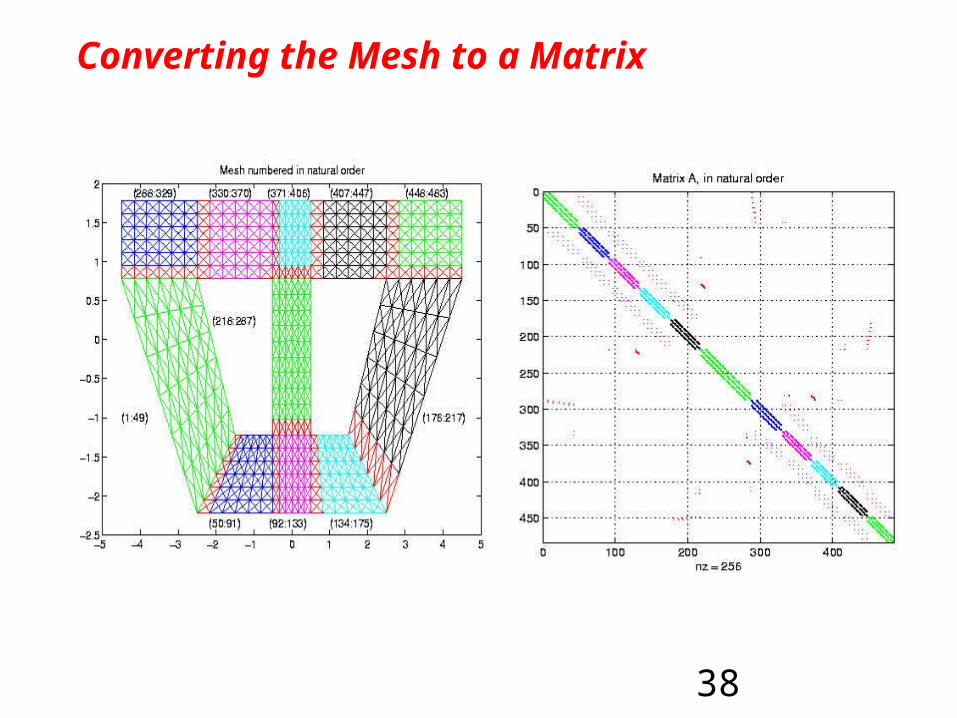
Converting the Mesh to a Matrix
39
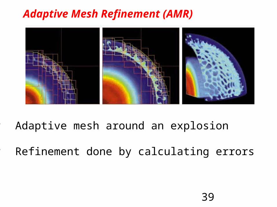
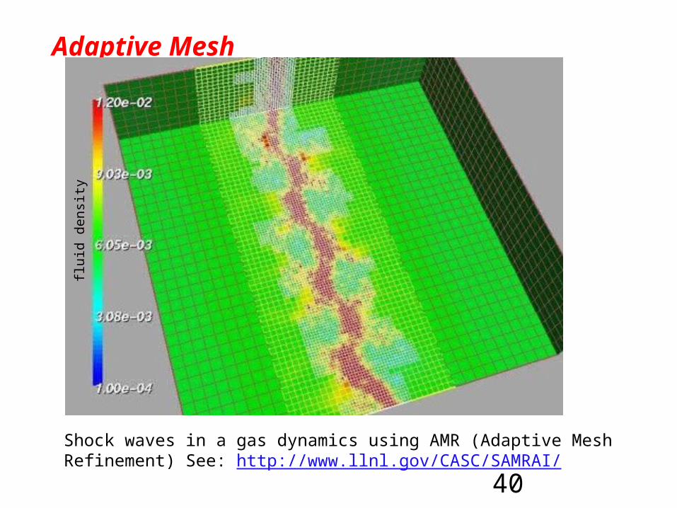
Adaptive Mesh Refinement (AMR)
• Adaptive mesh around an explosion
• Refinement done by calculating errors
40
Adaptive Mesh
Shock waves in a gas dynamics using AMR (Adaptive Mesh Refinement) See: http://www.llnl.gov/CASC/SAMRAI/
flu
id d
ensi
t y
41
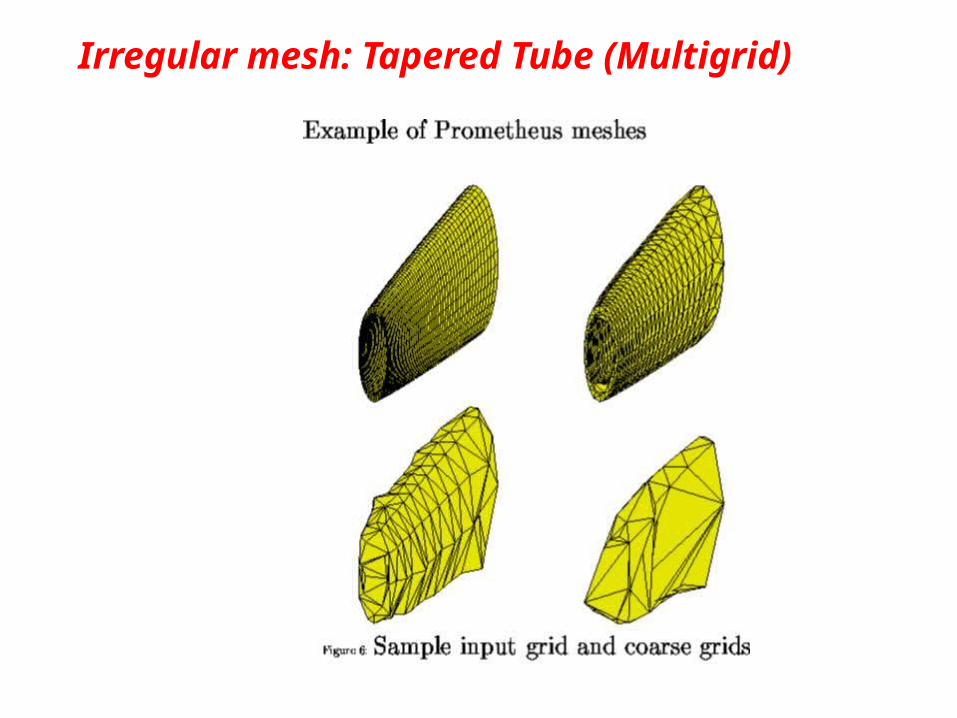
Irregular mesh: Tapered Tube (Multigrid)
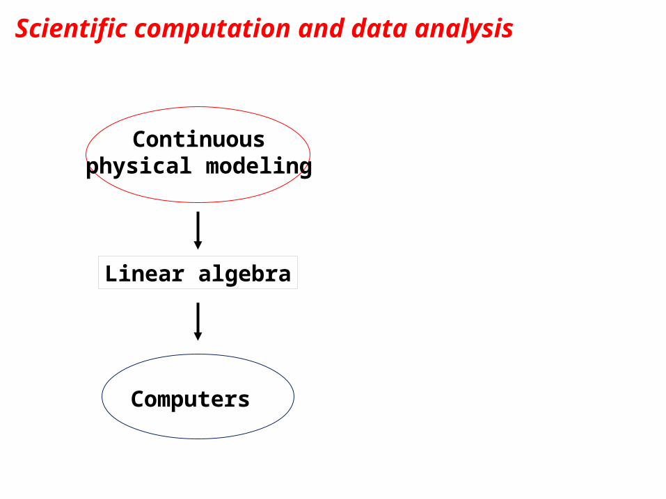
Scientific computation and data analysis
Computers
Continuousphysical modeling
Linear algebra
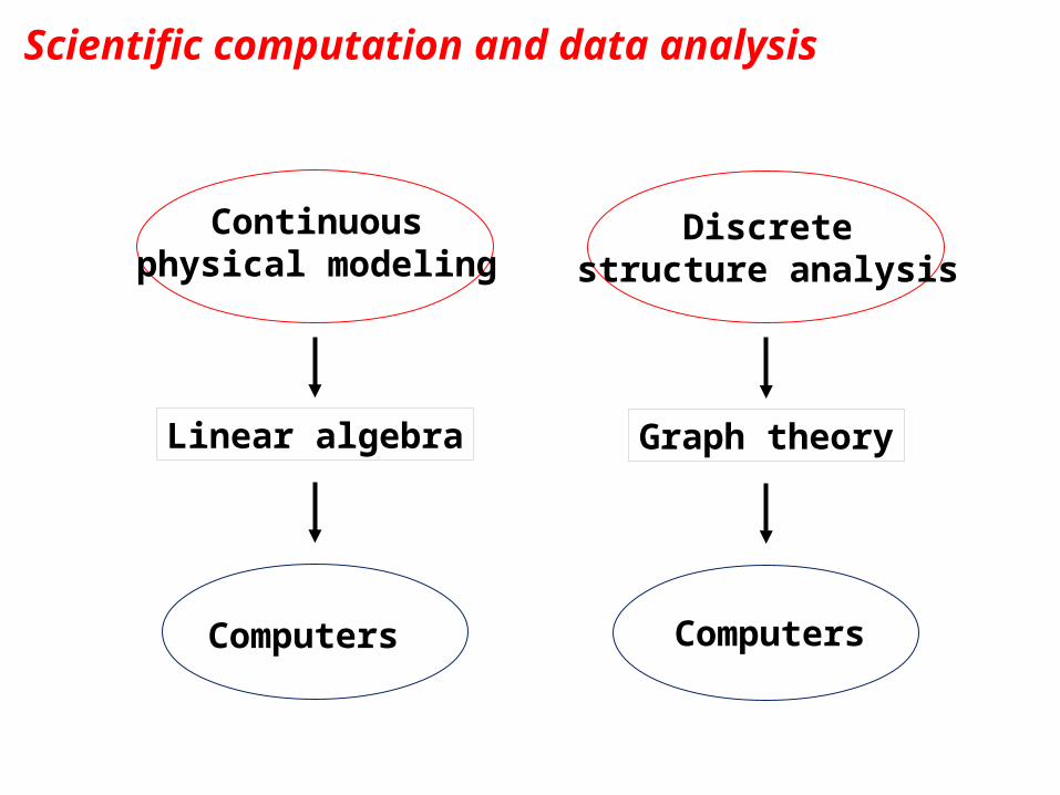
Scientific computation and data analysis
Computers
Continuousphysical modeling
Linear algebra
Discretestructure analysis
Graph theory
Computers
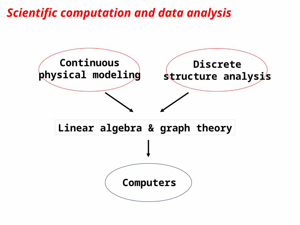
Scientific computation and data analysis
Continuousphysical modeling
Linear algebra & graph theory
Discretestructure analysis
Computers