Embed Size (px)
Citation preview

Connection Demand Prediction for the Design of Precast Concrete Wall Panels Subjected
to Blast Loads
by
Anthony Clark Consunji
A thesis submitted to the Graduate Faculty of
Auburn University
in partial fulfillment of the
requirements for the Degree of
Master of Science
Auburn, Alabama
May 10, 2015
Single-Degree-Of-Freedom, Blast, Dynamic Reactions, Connections, Precast Wall Panels, Finite
Element Modeling
Copyright 2015 by Anthony Consunji
Approved by
James S. Davidson, Committee Chair, Professor of Civil Engineering
Justin D. Marshall, Associate Professor of Civil Engineering
Robert W. Barnes, Associate Professor of Civil Engineering

ii
Abstract
One challenge in design of structures for highly impulsive loading is accurately predicting
the peak transient shear and the corresponding connection force demand at supports. Single-
degree-of-freedom (SDOF) approaches are commonly used for analyzing the maximum dynamic
deflections and flexural moments, and have been extensively demonstrated to be reasonably
accurate for those purposes. However, the typical SDOF methodology assumes that the inertia
distribution under the dynamic loading is the same as the simple static deflection shape, which
may not be accurate for analyzing the transient shear. The difficulty primarily comes from (1) the
complex distribution of inertia forces that vary spatially and temporally and are not easily
approximated, (2) the peak transient shear forces tend to be high intensity for only a very short
duration, and (3) strain rate effects associated with the short duration shear and connection
response are not easily quantified or are otherwise unknown. To circumvent these challenges,
engineers often use the design flexural capacity (i.e. ultimate resistance) as the basis for the shear
and connection design forces. Although this equivalent static reaction force approach is used for
many blast design applications, it must be recognized that it is not founded on solving the equation
of motion, and therefore cannot predict true demand. The need for an accurate yet simple equation
of motion based approach for predicting shear and connection demand is critical for relatively
slender precast panels.
This thesis presents the methodology developed for predicting the shear and connection
forces associated with blast loaded slender precast panels typically used for exterior wall systems

iii
and facades. High fidelity finite element modeling is used to understand the intricate dynamic
response mechanics involved, and the modeling and derived analytical SDOF approaches are
compared to full-scale explosion load test data.
It was found through this research that SDOF dynamic reaction force methodology can
predict the reaction forces with reasonable accuracy. Also, it was found that for a range of blast
loads magnitudes, dynamic reaction forces exceed the equivalent static reaction force based on the
flexural resistance that engineers use to design precast wall connections. Additional research is
required however to determine if strain rate effects sufficiently compensate for the difference
between the peak dynamic force and the equivalent static reaction force in which the connections
are designed.

iv
Acknowledgments
I would like to thank my advising Professor Dr. Davidson as well as Dr. Barnes and Dr.
Marshall their guidance and support over the past few years which have really helped myself grow
as a person professionally and personally. I would like to thank my friends both in and out of the
structures department: Patrick Koch, Zach Skinner, Mitchell Tribout, Neil Tiwari, Taylor
Rawlinson, Will Childs, Jonathan Campbell, Dave Mante, Michael Langley, Joey Nickerson,
Jamieson Matthews, Drew Eiland and Todd Deason. I told Zach when I started the Master’s
program that I would sneak the word mongoose in my thesis, so there it is; ha. Lastly, I would like
to thank my parents Rey and Jenifer Consunji because if it wasn’t for their continued support, none
of this would be possible.

v
Table of Contents
Abstract ........................................................................................................................................... ii
List of Tables ................................................................................................................................ vii
List of Illustrations ....................................................................................................................... viii
List of Abbreviations and Symbols................................................................................................ xi
Chapter 1. Introduction ............................................................................................................... 1
1.1 Overview ...................................................................................................................... 1
1.2 Objectives ..................................................................................................................... 4
1.3 Scope of Work and Methodology ................................................................................. 4
1.4 Organization of Thesis.................................................................................................. 5
Chapter 2. Literature Review...................................................................................................... 6
2.1 Introduction .................................................................................................................. 6
2.2 Basic Approach to Blast Design ................................................................................... 6
2.3 Blast Loads ................................................................................................................... 7
2.4 Cast-in-Place Panels ................................................................................................... 10
2.5 Precast and Precast Sandwich Panels ......................................................................... 11
2.6 Precast Panel Connections .......................................................................................... 13
2.7 Equivalent Static Reaction Force ............................................................................... 17
2.8 Dynamic Reaction Force Prediction Methodology .................................................... 18
2.8.1 Biggs ........................................................................................................................... 18
2.8.2 Ardila-Giraldo ............................................................................................................ 21
2.8.3 Keenan ........................................................................................................................ 26
2.8.4 Krauthammer .............................................................................................................. 31
2.8.5 Magnusson .................................................................................................................. 33
2.8.6 Adaros, Wood and Eepoel .......................................................................................... 34
2.8.7 Oswald ........................................................................................................................ 38
2.9 Material Behavior at High Strain Rates ...................................................................... 40
2.10 Blast Resistant Precast Wall Panel Connection Design ............................................. 44
Chapter 3. Computer Modeling and Analysis Methodology .................................................... 49

vi
3.1 Overview .................................................................................................................... 49
3.2 Single Degree of Freedom Analysis ........................................................................... 50
3.2.1 General SDOF Methodology ...................................................................................... 50
3.2.2 Central Difference Numerical Method ....................................................................... 54
3.3 Finite Element Analysis.............................................................................................. 56
Chapter 4. Results ..................................................................................................................... 60
4.1 Overview .................................................................................................................... 60
4.2 Investigation of Inertia Force Distribution Associated with Elastic Beams ............... 62
4.3 Comparisons of Dynamic Reaction Force Results from SDOF and FE Full Model
Analyses .................................................................................................................................... 73
4.4 Comparison of AFRL Connection Demand Test Data to SDOF Reaction Prediction83
4.5 Limitations of Connection Design Based on the Flexural Resistance ...................... 101
Chapter 5. Conclusions and Recommendations for Future Work .......................................... 106
References ............................................................................................................................... 109
Appendix A. Users Guide on Creating SBEDS and LS-DYNA Keyword Input Files .............. 112
Appendix B. Sample LS-DYNA Keyword File ......................................................................... 133

vii
List of Tables
Table 2-1 Blast Affected Beam Data (Adaros, Wood and Eepoel 2013) ..................................... 36
Table 2-2 Material Strength Increase Factors for Structural Steel (USACE 2008) ...................... 43
Table 4-1 Distance to the Inertia Force and the Ardila-Giraldo Dynamic Reaction Equation
Coefficients through the First 18 ms ............................................................................................. 69
Table 4-2 Biggs’ Distance to the Inertia Force Resultant Assumption and Corresponding
Dynamic Reaction Equation Coefficients ..................................................................................... 69
Table 4-3 Test Panel’s Support Rotation for Varying Charge Weights and Standoff Distances . 74
Table 4-4 AFRL Test Sandwich Panel Details ............................................................................. 86
Table 4-5 Comparison of Equivalent Static Reaction to Peak Reactions ................................... 103

viii
List of Illustrations
Figure 2-1 Generalized Reflected Pressure ..................................................................................... 9
Figure 2-2 Idealized Blast Pressure History (USACE 2008) ........................................................ 10
Figure 2-3 Typical Clip Angle Precast Wall Connection (Adapted from The Constructor 2014) 12
Figure 2-4 Welded Flat Plate Precast Wall Connection (Adapted from The Constructor 2014) . 12
Figure 2-5 Insulated Sandwich Panel ........................................................................................... 13
Figure 2-6 Precast Wall Panel Slotted Inserts (Dayton Superior Corportation 2014) .................. 14
Figure 2-7 Halfen Precast Wall Panel Channel Insert (Halfen USA 2014) .................................. 14
Figure 2-8 Slotted Strap PSA Connection Welded to a Slab Embed (Oswald and Bazan 2013) . 15
Figure 2-9 Grouted Sleeve Anchor Connection (Oswald and Bazan 2013) ................................. 16
Figure 2-10 Free Body Diagram of the Equivalent Static Reaction Force ................................... 17
Figure 2-11 Free Body Diagram Relating Resistance to Plastic Moment .................................... 18
Figure 2-12 Free Body Diagrams Used to Derive Dynamic Reaction Force Equations .............. 19
Figure 2-13. Differences in the Deformed Shapes between Dynamic and Static Tests of Beams
(Ardila-Giraldo 2010) ................................................................................................................... 22
Figure 2-14 Free Body Diagram for the Modified Dynamic Reaction Force Equation ............... 23
Figure 2-15 Deflected Shapes of Fixed-Fixed Beams at the Time of Maximum Shear in the
Initial Phase Calculated Using FE for Several Beams (Ardila-Giraldo 2010) ............................. 25
Figure 2-16 Binlinear Envelope Showing Variable of β with Time in Initial Phase of Fixed-fixed
Beams (Ardila-Giraldo 2010) ....................................................................................................... 25
Figure 2-17 DIF Equations as Functions of Time (Keenan 1976) ................................................ 27
Figure 2-18 Maximum DIF Chart (Keenan 1976) ........................................................................ 29
Figure 2-19 Comparison between Measured and Predicted Support Shears (Keenan 1976) ....... 30
Figure 2-20 Typical Dynamic Shear History (Keenan 1976) ....................................................... 31
Figure 2-21 Comparison between the Registered and Calculated Support Reactions for Beam
B140F-D2 (Magnusson 2007) ...................................................................................................... 34
Figure 2-22 Comparison between the Registered and Calculated Support Reactions for Beam
B140F-D3 (Magnusson 2007) ...................................................................................................... 34
Figure 2-23 Inertia Forces along Span through Time (Adaros, Wood and Eepoel 2013) ............ 35

ix
Figure 2-24 Variation of RAF with α (T/td) and beta (Po/Rm) (Adaros, Wood and Eepoel 2013) 37
Figure 2-25 Variation of RAF with Ductility and α (Adaros, Wood and Eepoel 2013) .............. 38
Figure 2-26 Rate Effect Curve for Concrete in Tension (Malvar and Crawford 1998a) .............. 41
Figure 2-27 Rate Effect Curve for Steel Reinforcing bars (Malvar and Crawford 1998b) .......... 42
Figure 2-28 Strain Rate vs. Concrete Ultimate Compressive Strength (USACE 2008) ............... 44
Figure 3-1 (a) Displacement representation of sandwich panel subjected to blast load and (b)
Equivalent single degree of freedom system (Newberry 2011) .................................................... 53
Figure 3-2 Screenshot of SDOF central difference method in Microsoft Excel spreadsheet format
....................................................................................................................................................... 56
Figure 3-3 Finite Element Reinforced Concrete Wall Panel Model ............................................. 57
Figure 4-1 Elasto-plastic Resistance Function Used in SDOF Analysis ...................................... 60
Figure 4-2 Displacement along the Span of an Elastic Beam through First 1 ms ........................ 64
Figure 4-3 Displacement along the Span of an Elastic Beam through First 12 ms ...................... 64
Figure 4-4 Midspan Deflection vs Time ....................................................................................... 65
Figure 4-5 Acceleration along the Span of an Elastic Beam through First 1.0 ms ....................... 66
Figure 4-6 Acceleration along the Span of an Elastic Beam through First 12 ms ........................ 67
Figure 4-7 Acceleration along the Span of an Elastic Beam through 12-24 ms ........................... 68
Figure 4-8 Distance to the Inertia Force Centroid for an Elastic Beam subjected to blast loads . 70
Figure 4-9 Reaction Force Histories for Elastic Beam subjected to Blast Loading ..................... 71
Figure 4-10 Ardila-Giraldo Beta Bilinear Envelope Modified SDOF Reaction Force History 11.1
psi, 93 psi-ms. First 30 ms of Analysis ......................................................................................... 72
Figure 4-11 Reaction Force History Comparison. Loading 1: 7.7psi, 63.6psi-ms ....................... 75
Figure 4-12 Reaction Force History Comparison. Loading 2: 23.5 psi, 143 psi-ms .................... 77
Figure 4-13 Reaction Force History Comparison. Loading 3: 47.8 psi, 198 psi-ms .................... 78
Figure 4-14 Reaction Force History Comparison. Loading 4: 34.1 psi, 199 psi-ms .................... 79
Figure 4-15 Reaction Force History Comparison. Loading 5: 73.5 psi, 278.4 psi-ms ................. 80
Figure 4-16 Reaction Force History Comparison. Loading 6: 91 psi, 327.7 psi-ms .................... 80
Figure 4-17 Reaction Force History Comparison. Loading 7: 156 psi, 408.6 psi-ms .................. 81
Figure 4-18 Reaction Force History Comparison. Loading 8: 462 psi, 732.9 psi-ms .................. 81
Figure 4-19 Test Set Up for Full-scale dynamic tests with single span reaction structure (left) and
multi-span reaction structure (right) ............................................................................................. 84
Figure 4-20 Single Span TCA Blast Specimens (Naito et al. 2011) ............................................. 85
Figure 4-21 Specimen M3 Details (Naito et al. 2011) .................................................................. 85
Figure 4-22 Specimen M4 Details (Naito et al. 2011) .................................................................. 86

x
Figure 4-23 Instrumentation Single-Span Panels (Naito et al. 2011) ........................................... 87
Figure 4-24 Single-Span Wall Setup (Naito et al. 2011) .............................................................. 88
Figure 4-25 Single-Span Top Connection Detail (Naito et al. 2011) ........................................... 89
Figure 4-26 Variable Input Comparisons of Panel M3 reaction force data first 20 ms of response
....................................................................................................................................................... 90
Figure 4-27 Variable Input Comparisons of Panel M3 reaction force data full response ............ 91
Figure 4-28 Measured Reflected Pressures and Calculated Impulses, Test 1 .............................. 94
Figure 4-29 Reaction Force History Comparison of SDOF Methodology and Measured Reaction
Force Data for Precast Wall Panel M3, Test 1 .............................................................................. 95
Figure 4-30 Reaction Force History Comparison of SDOF Methodology and Measured Reaction
Force Data for Precast Wall Panel M4, Test 1 .............................................................................. 96
Figure 4-31 Measured Reflected Pressures and Calculated Impulses, Test 2 .............................. 97
Figure 4-32 Reaction Force History Comparison of SDOF Methodology and Measured Reaction
Force Data for Precast Wall Panel M3, Test 2 .............................................................................. 98
Figure 4-33 Reaction Force History Comparison of SDOF Methodology and Measured Reaction
Force Data for Precast Wall Panel M4, Test 2 .............................................................................. 99
Figure 4-34 Peak Reaction Exceedance of ESR at Varying Levels of Support Rotation ........... 103

xi
List of Abbreviations and Symbols
AFRL Air Force Research Laboratory
ASCE American Society of Civil Engineers
α Dynamic Reaction Resistance Coefficient
B Peak Blast Load
β Damping Ratio AND Dynamic Reaction Force Coefficient
DIF Dynamic Increase Factor
DoD Department of Defense
ESR Equivalent Static Reaction (also ESS)
ESS Equivalent Static Shear (see ESR)
F Applied Load
FE Finite Element
HD Heat of Detonation of TNT
HDEXP Heat of Detonation of the Explosive
I Inertia Force Resultant
L Span Length
LSTC Livermore Software Technology Corporation
Mp Moment that Induces Plastic Material Behavior
Mm Moment at Midspan
Mend Moment at End
MRP Measured Reflected Pressure
PDC Protective Design Center (part of the USACE)
RAF Reaction Amplification Factor
RFH Reaction Force History
R Flexural Resistance
Ru Total Ultimate Flexural Resistance
ru Static Ultimate Flexural Resistance per unit length
SBEDS SDOF Blast Effects Design Spreadsheet

xii
SDOF Single Degree of Freedom
SIF Average Strength Increase Factor (for steel)
SSIF Concrete Static Strength Increase Factor
TNT Trinitrotoluene
t Time
Tn Fundamental Period of Vibration
US United States
USACE United States Army Corps of Engineers
V Dynamic Reaction Force
Vu Equivalent Static Reaction Load from the Ultimate Resistance
WE Equivalent Weight of TNT
WEXP Weight of the Explosive
x Distance Along Span
�� Distance to Centroid of Half Span Inertia Force Distribution

1
Chapter 1. Introduction
1.1 Overview
Extremist organizations around the world use explosives to inflict as much damage as they
can to their enemies. It has become commonplace for these groups to attack the United States’
facilities abroad. The U.S. has military bases and embassies all over the world. And in many
circumstances, these facilities are located in highly volatile surroundings. By keeping structures in
these zones, the United States exposes strategically important buildings and their occupants to
explosions. To combat this, research of structural response to different impulse loads has increased
in recent years. In addition to defense, the petrochemical industry also must be wary of accidental
explosions because of the danger associated with highly volatile petrochemical accidents (ASCE
2010). It is the responsibility of the structural engineer to provide protection of a structures’
occupants from blast loads if it has a reasonable chance of being subjected to an explosion.
Engineers also must make their designs economical. While providing life safety is the
foremost concern in design, it is the engineer’s job to minimize costs, materials, and construction
time. Some construction contractors complain about how expensive connections are to produce
and install. Specifically, contractors complain about the costs of making and installing the elements
that connect precast wall panels to the supporting elements of the structure. They claim that the
connections become uneconomical because the connections are designed according to excessive
loads. They also claim that the designer’s methods of determining the design loads for the
connection are unknown.
Blast loads, like earthquake loads, are considered to be dynamic loads. Dynamic loads are
different from typical static loads because in a dynamic scenario, the applied forces external are
not immediately balanced by other external forces because of the temporal change in position.

2
According to Newton’s second law, the external forces are balanced by the acceleration of mass
(or the inertia force). Due to the huge amounts of energy in earthquakes and blasts, it is impossible
to restrain a structure so much that it does not react dynamically to these loads. Because dynamic
loads cause the structure to move, the inertia forces must be taken into account when performing
an analysis. Blast research has shown that short-duration high-magnitude loading conditions
caused by blast result in significantly different structural response than static loads, slowly moving
line loads, and even earthquake loads (Krauthammer 1999). Explosive loads are typically applied
to structures at rates about 1000 times faster than earthquake induced loads, and the corresponding
structural response frequencies can be much higher than those induced through conventional loads.
In addition, short-duration dynamic loads can move structural elements so quickly that they can
cause sudden increases in stress. The sudden increases in stress cause high strain rates that affect
the strength and durability of structural materials, the bond relationships for reinforcement, the
failure modes, and the structural energy absorption capabilities. Because of the differences
outlined here between structural response due to blast effects and structural response due to
conventional loadings and earthquakes, blast design must be considered independently.
The precast concrete industry has made great strides recently. Using precast wall panels
has several advantages, and the most important advantage that precast wall panels provide is the
increase in economy. The economy is improved by providing faster and simpler construction, and
more consistent production methods. When construction is simple and is able to be completed
quickly, money is saved. Because concrete wall panels are cast in a precast plant, it provides strict
control in the production of the precast wall, which leads to a better overall product. Also, because
of the strict control in precast construction, the precast panels have the capability to be prestressed
and/or insulated (Nickerson, Consunji and Davidson 2014). The prestressing allows the panels to

3
be transported without cracking, and the insulation layer within the concrete wythes provides
thermal insulation, so the occupant can save money on heating and cooling costs. Higher quality
and cheaper is the obvious choice for many when available, so as precast wall panels become more
and more common, it is important to be able to design them appropriately.
Recently, the U.S. Department of Defense has shown greater interest in using precast wall
panels, specifically precast insulated foam sandwich panels, for all types of construction purposes.
This includes structures that may be subject to blast loads. The primary advantage of monolithic
concrete wall construction over precast concrete wall construction is the strength and structural
integrity provided by the solid-through construction. Precast concrete panels are connected to the
supporting structure at discrete points and experience the entirety of the maximum dynamic
connection forces locally. The Protective Design Center of the U.S. Army Corps of Engineers
(2008) say that most observed failures of structural components subjected to blast loads have
occurred at the connections.
For years, designers have used single degree of freedom (SDOF) methods to calculate the
effects of blast loads on composite and non-composite concrete wall sections. The quantities that
designers use to assess the amount of damage sustained are maximum deflections, rotations, and
reaction forces. Other research has found that these SDOF calculations accurately predict
displacements and rotations of the wall sections against test data. This includes both real testing
and computationally intensive FE analysis. Additionally, independent research has produced new
methods of calculating the reaction forces.
Recent research shows that SDOF prediction methodology makes an incorrect assumption
about the inertia force distribution. The complex distribution of inertia forces that vary spatially
are not fully understood nor easily approximated. Calculated dynamic reactions through SDOF

4
methods are not presently used to determine the force demand for precast wall connections subject
to blast loads. Instead, the equivalent static reaction is used to determine the factored load used in
precast wall connection design. Calculated and measured dynamic reaction forces are observed to
commonly exceed the forces used to design the connections. Still, some connections designed for
the equivalent static reaction have been shown to survive blast loads and the forces associated
therein while other connections have not. Also, the peak transient reaction and shear forces tend
to be high intensity for only a very short duration, and strain rate effects associated with the short
duration shear and connection response are not easily quantified or are otherwise unknown.
1.2 Objectives
There are three objectives of this research:
1) Develop a comprehensive understanding of the mechanics involved in the reaction force
variation through time for precast concrete panels subjected to blast loads;
2) Evaluate the accuracy and limitations of currently used SDOF methodologies for predicting
connection demand for the design of precast concrete panels subjected to blast loads; and
3) Define the limitations of using the static flexural strength as the basis for connection design
of precast concrete panels for blast loading.
1.3 Scope of Work and Methodology
The work is limited to investigating the forces of single span precast concrete wall panels
subject to blast loads with connections that allow rotation at both supports. Partially restrained and
fixed supports were not fully investigated but were considered when comparative analyses were
performed. Also, only one-way flexural action of the panel was investigated. Tension membrane
effects and multispan wall panels were not considered in this research. Several different
magnitudes of blast parameters were considered and several types of panels were considered in

5
order to provide a comprehensive analysis. To achieve the objectives, SDOF and finite element
results were compared to investigate the further the understanding of the mechanics involved in
the reaction force variation through time. LS-DYNA is used in this research for high fidelity finite
element simulations. SDOF methodology and the central difference numerical method were coded
into spreadsheets. The results of the SDOF spreadsheet were checked with the PDC blast effects
SDOF calculator SBEDS. Lastly, SDOF methodologies were assessed against the results of full
scale blast tests conducted by the Air Force Research Laboratory to evaluate their accuracy in
determining the connection force demand.
1.4 Organization of Thesis
This report contains five chapters. Chapter 1 states the objectives, scope, methodology, and
report organization. Chapter 2 provides a literature review and background of relevant history and
analytical information. Chapter 3 discusses the Single Degree Of Freedom methodology and
Finite Element Modeling. Chapter 4 describes the single degree of freedom prediction models and
comparison to finite element analyses and full-scale dynamic tests. Chapter 5 summarizes the
report and provides conclusions and recommendation for future work.

6
Chapter 2. Literature Review
2.1 Introduction
In this section, literature on several subjects related to blast pressures, concrete construction
methods including precast wall panel connection design and precast sandwich panel design for
blasts, material behavior at high strain rates, and FE methods for reinforced concrete are reviewed
in order to gain a comprehensive knowledge on the most relevant and current research related to
the research to be discussed in the subsequent chapters. Engineers, both researchers and designers,
have been calculating reaction forces based on the method John Biggs presented in his 1964
textbook since its inception. Some researchers made modifications on the Biggs dynamic reaction
calculation method and others developed entirely new methods to calculate dynamic reaction
forces.
2.2 Basic Approach to Blast Design
Newmark’s ASCE wrote that the designer shall not design a blast-resistant structure with
the deflection of it in mind, but instead suggests that designers should design for an equivalent
static loading. In the self-description of Unified Facilities Criteria (UFC) document “Structures to
Resist the Effects of Accidental Explosions” or UFC 3-340-02, as it is commonly referred to as, it
states that “UFC 3-340-02 presents methods of design for protective construction … [and] In so
doing, it establishes design procedures and construction techniques whereby propagation of
explosion or mass detonation can be prevented and personnel and valuable equipment can be
protected (2008).” UFC 3-340-02 states that the purpose of the document is to predict response,
and other manuals should be consulted to establish the safety criteria.
The objective of UFC 3-340-02 is based around protecting the acceptor system, or the
structural system that is subjected to blast loads. It defines the acceptor system as being:

7
“composed of the personnel, equipment, or explosives that require protection. Acceptable
injury to personnel or damage to equipment, and sensitivity of the acceptor explosive(s),
establishes the degree of protection that must be provided by the protective structure. The
type of the protective structure and capacity of it are selected to produce a balanced design
with respect to the degree of protection required by the acceptor and the hazardous output
of the donor.”
The two ways designers can protect the intended target is through the use of distance, or how far
away the origin of the blast is from the affected structure, and the level to which the protective
structure is designed. Overall, the goal of the design engineer is to dissipate the blast energy that
is imparted to the building without collapse. Newmark (1953) suggests that by ensuring that the
energy dissipation of the element exceeds the input energy of the load, a structural element will be
adequately designed to resist an impulsive load. Impulsive loads have very short durations when
compared to the natural period of vibration of the loaded element and typically have high peak
loads. Biggs (1964) defines a load as impulsive if the duration is less than 0.1 times the natural
period of the system.
2.3 Blast Loads
An explosion is a violent load scenario that occurs due to the release of large amounts of
energy in a very short amount of time (Tedesco, McDougal and Ross 1999). This energy could
come in the form of a chemical reaction as in explosive ordnances or from the rupture of high
pressure gas cylinders. Trinitrotoluene (TNT) equivalence is used to compare the effects of

8
different explosive charge materials. The equation used for calculating the TNT equivalence based
on weight is as follows:
D
EXPE EXPD
TNT
HW W
H (2-1)
where WE is the TNT equivalent weight, WEXP is the weight of the explosive, HDEXP is the heat of
detonation of the explosive, and HD is the heat of detonation of TNT.
When an explosion occurs, an increase in the ambient air pressure, called overpressure,
presents itself as a shock front that propagates spherically from the source. When the shock front
comes in contact with a surface normal to itself, an instantaneous reflected pressure is experienced
by the surface that is twice the overpressure plus the dynamic pressure. This peak positive pressure
can be quite large and decays nonlinearly to a pressure below the ambient air pressure. The period
of positive pressure that the surface experiences is called the positive phase. The negative phase
occurs when the pressure experience by the surface is negative (e.g. suction). The negative phase,
although much smaller in magnitude than the positive phase, affects the surface for a relatively
extended amount of time compared to the positive phase (USACE 2008). Figure 2-1 illustrates
the basic shape, relative magnitudes, and durations for the positive and negative phases of a
pressure wave created by an explosion.

9
Figure 2-1 Generalized Reflected Pressure
Structures at risk are designed to resist the reflected pressure of a blast load. Peak positive pressure
and impulse (area under the pressure vs. time curve) are the most important considerations in
design of structures for impulse loads. A conservative assumption used in design is to only
consider the positive phase, since neglect of the negative phase “will cause similar or somewhat
more structural response”, while taking into account the “ratio of the blast load duration to the
natural period of the structural component” (USACE 2008). The most common simplification is
the idealized right triangle blast pressure history. This idealizes the blast pressure history as an
instantaneous equivalent peak pressure followed by a linear decay of pressure that achieves an
equivalent impulse. This idealization can be seen in Figure 2-2.

10
Figure 2-2 Idealized Blast Pressure History (USACE 2008)
2.4 Cast-in-Place Panels
Cast-in-place concrete panels are typically constructed as load-bearing walls or as panels on
a reinforced concrete frame building (Oswald and Bazan 2013). These panels can be constructed
with conventional reinforcing steel, welded wire reinforcement, or prestressed reinforcing strands,
but most are constructed with conventional steel reinforcing bars. The walls are built with
reinforcing steel across all joints so the wall acts as a monolithic component with the supporting
elements so that there are no potential weak points in that area structure. Cast-in-place concrete
has traditionally been used for blast-resistant design because the walls are continuously connected
to the supporting frame, and therefore have a very robust connection to the supporting structure.
Cast-in-place concrete can develop much higher blast resistances through i.e. tension and
compression membrane response compared to their “basic” blast resistance in flexural response.
Tension and compression membrane response occurs because the cast-in-place construction
restricts in-plane movement at the edges of the panel. However, compression membrane response
requires very rigid supports that can develop arching in the wall and tension membrane response

11
only develops at large displacements, so these types of response are not usually assumed for blast
design.
2.5 Precast and Precast Sandwich Panels
Precast panels are cast in a manufacturing plant and transported to the job site (Oswald and
Bazan 2013). The precast manufacturing system offers more options in the construction of the
panels, tighter construction tolerances, and more thorough inspection during construction. Precast
panels can be manufactured with conventional reinforcing steel or prestressing strands. The panels
can be solid panels, or insulated panels with a built-in layer of insulation which are also known as
sandwich panels. Also, different types of architectural finishes are available for application to the
panels before transporting to the job site. Typically, transportation restrictions limit the size and
weight of the panels. A mobile precasting setup can be constructed for very large projects, where
the precast manufacturing equipment is disassembled and moved after the project is complete.
Precast panels are structurally identical to cast-in-place panels, except they are connected to
the supporting structure at discrete points with connections. The connections typically do not
provide any in-plane restraint, and therefore do not allow the panels to develop compression or
tension membrane strength. When this happens, the connections are more susceptible to failure.
Shims between panels can be used to allow the panels to support their own gravity load in low-
rise buildings. Precast panels can also be designed as load-bearing to resist the roof load in low-
rise buildings. The lateral connections are the primary concern for blast-resistant design, since the
connections transfer the reaction forces from the blast load on the panel into the supporting
structure. Figure 2-3 shows a typical clip angle construction that provides lateral support for
panels. The precast panel and floor slab each have cast-in-place embedded plates that are

12
connected with the clip angle in the field after the panel is positioned. A welded flat plate
connection can also be used instead of a clip angle, as shown in Figure 2-4.
Figure 2-3 Typical Clip Angle Precast Wall Connection (Adapted from The Constructor
2014)
Figure 2-4 Welded Flat Plate Precast Wall Connection (Adapted from The Constructor
2014)
Sandwich panels are commonly used for both exterior and interior walls, and also can be
designed solely for cladding or as load-bearing members (PCI 1997). Sandwich panels have
become popular due to their energy efficiency (Newberry 2011). The amount of mass provided by

13
the concrete layers along with the layer of foam provide the designer with a wide variety of
thermally-efficient options for walls. Sandwich panels are primarily designed to withstand
handling, transportation, and construction loads. These conditions most often provide the largest
stresses within the service life of the sandwich panel. The typical configuration of concrete
sandwich wall panels is two wythes (i.e. layers) of reinforced concrete, either conventionally
reinforced or prestressed, separated by a layer of insulating foam with connectors that secure the
concrete wythes through the foam. An example of a precast concrete insulated sandwich panel is
shown in Figure 2-5. The disadvantage of precast construction for blast design is that it lacks the
redundant connections that cast-in-place construction provides.
Figure 2-5 Insulated Sandwich Panel
2.6 Precast Panel Connections
Precast wall panel connections are extremely important in precast wall panel construction
for blast protection. But, in addition to providing strength for blast loads, they must also ressit the
gravity, wind, earthquake, and temperature effects. In order to avoid cracking caused by
temperature-induced strains, and to make placement on the structure easier, precast panels are
often connected with slotted connections that allow horizontal or vertical movement (Oswald and
Bazan 2013). Figure 2-6 and Figure 2-7 show slotted inserts and channel inserts, respectively.
These connections have an insert or channel with a slot that is cast into the precast slab. A bolt or
slotted plate is placed into the slot after the panel is placed and connected to a plate or angle in the
supporting structure. Figure 2-8 shows a photograph of a slotted strap from a PSA connection

14
welded to an embedded plate in the structure. Blast resistant panels that are longer than 30 ft may
need to accept temperature-induced cracking if slotted connections do not have the required
capacity.
Figure 2-6 Precast Wall Panel Slotted Inserts (Dayton Superior Corportation 2014)
Figure 2-7 Halfen Precast Wall Panel Channel Insert (Halfen USA 2014)

15
Figure 2-8 Slotted Strap PSA Connection Welded to a Slab Embed (Oswald and Bazan
2013)
Connections between precast panels and the supporting structure can also be made with
spliced reinforcing steel (Oswald and Bazan 2013). This is possible when the reinforcing steel is
able to be anchored and fully developed within concrete slabs. Figure 2-9 shows a grouted sleeve
anchor connection. The grouted connection provides continuity of reinforcing steel from a slab
into a precast wall panel. The foundation slab is cast first with the rebar extending vertically out
of the slab. The splice sleeve and panel reinforcement extending into the coupler are cast into the
panel. After the panel is in place, the sleeve is filled with grout that splices the reinforcing bars to
the slab and panel. Not only is this connection much stronger than a bolted or welded angle
connection, it provides much more redundancy and structural integrity than a standard precast wall
panel connection. It is often used for wall-to-slab connections that have very high connection
loads, such as load bearing shear walls in seismic zones and environments where blasts are likely.

16
Figure 2-9 Grouted Sleeve Anchor Connection (Oswald and Bazan 2013)
An advantage of cast-in-place concrete over precast is that it does not have discrete
connection points between the wall and supporting structure that act as weak points (Oswald and
Bazan 2013). Connections between precast panels can be designed so that they are not weak points,
but the connections are still susceptible to being possible points of weakness if there are flaws in
construction. The installation and detailing of the connections of precast panels must be done
correctly. The continuous connection between wall and structure in cast-in-place concrete is
inherently more redundant and provides more structural integrity than discrete connections used
to connect precast panels to the structure. The ability to use the same precast wall panels and

17
connections repeatedly throughout a building is important for the cost-effectiveness of precast
panels.
The construction costs of cast-in-place and precast construction are usually similar because
of the costs associated with the precast panel transportation and installation (Oswald and Bazan
2013). The primary advantages of precast panels are greater flexibility in construction, better
finishes, insulating layers within panels, faster on-site construction time, and better quality control.
Because of these advantages, the large majority of concrete wall construction for office and
industrial buildings in the U.S. involves precast (including tilt-up) construction.
2.7 Equivalent Static Reaction Force
The equivalent static reaction is the force at the support when the component reaches its
maximum flexural resistance during dynamic flexural response (USACE 2008). The ultimate
flexural resistance is a function of the strength, amount and location of the reinforcement, the
thickness and strength of the concrete and the dimensions of the panels. The resistance has the
same spatial distribution as the applied load. The equation for calculating the equivalent static
reaction force is defined in Equation 2-2. The concept of the equivalent static reaction force is
illustrated in Figure 2-10. Equation 2-3 defines the equation for calculating the ultimate flexural
resistance for a simply supported beam if the moment that induces a plastic hinge is known.
2
uu
RV (2-2)
Figure 2-10 Free Body Diagram of the Equivalent Static Reaction Force
2
uR2
uR
uRw

18
8 p
u
MR
L
(2-3)
Figure 2-11 Free Body Diagram Relating Resistance to Plastic Moment
2.8 Dynamic Reaction Force Prediction Methodology
2.8.1 Biggs
The earliest documented and most widely recognized and used approach for finding the
dynamic reaction forces for beam-type systems is that of John Biggs, author of “Introduction to
Structural Dynamics” (1964). Biggs developed this approach by satisfying force and moment
equilibrium as the beam moves through time. The dynamics of a real structural element has no real
counterpart in the equivalent single degree of freedom system meaning that the spring force is not
equivalent to the actual dynamic reaction force, so a different approach must be used to determine
the dynamic reaction force. The dynamic reaction is calculated by summing the moments about
the centroid of the inertial force distribution. This is illustrated in the Figure 2-12 for a simply
supported beam subjected to a uniformly distributed dynamic load. The inertial force distribution
is assumed to have the exact same shape as the static deflected shape if the beam were loaded with
a uniformly distributed load. The rotational moment at the middle of the beam’s span, the reaction
force, and the dynamic loading induce moments about a chosen point, and depending on whether
2
uR
w
pM
0V 2
uR
2
L
4
L

19
the beam is considered to be in the elastic phase or the plastic phase, the centroid of the inertial
force distribution changes.
(a) (b)
Figure 2-12 Free Body Diagrams Used to Derive Dynamic Reaction Force Equations
(a) Full Span (b) Half Span
The inertia force is the passive force of mass to resist motion and will always act in the direction
opposite the mass’ acceleration, and is generally accounted for mathematically by the product of
mass and acceleration. The inertia force assumed here is distributed across the span of the beam
or slab with the same shape as the beam’s shape when loaded with a static uniform distributed
load. The assumption that the shape of the inertia force distribution is identical with the assumed
shape of the deflected beam is made because the motion is harmonic at any point along the span.
Because the motion is harmonic, the acceleration is directly proportional to the deflected shape.
This is defined by Equations 2-4 and 2-5. Hence, at any point along the beam, the intensity of the
inertia force is proportional to the ordinate of the deflected shape.
2( ) ( ) ( )y x y x A x (2-4)
3 3 4
4
16( ) ( 2 )
5x L x Lx x
L (2-5)

20
where ÿ is the acceleration at a point, ω is the natural frequency, y is the position at a point, A is
some constant value, ϕ is the shape function, L is the length, and x is distance along the beam.
To derive the dynamic reaction equation, the moments are summed about the inertia force
resultant which is found by using the deflected shape function (Equation 2-5) and assuming the
shear at midspan due to symmetry is negligible. The resulting equilibrium is defined by Equation
2-6. The dynamic bending moment at midspan is the function of the beam’s flexural deflection
and is accounted for at each time step in terms of the resistance. Equation 2-7 defines the flexural
resistance. By substituting and solving the equation through equilibrium, Equation 2-8 is obtained.
61 1 610
192 2 192 4m
L L LV M F
(2-6)
8 ( )( ) mM t
R tL
(2-7)
( ) 0.39 ( ) 0.11 ( )V t R t F t (2-8)
where x is distance along the beam, L is the span length, V is the dynamic reaction, Mm is the
moment at the midspan, F is the applied load, R is the flexural resistance, and t is time.
Presently, the only use for the Biggs dynamic reaction equation is the determination of
applied load to primary members such as girders and columns (USACE 2008). The secondary
framing members such as the beams, girts, purlins, and for the context of this research, the exterior
walls, receive the initial blast load then the SDOF analysis tool calculates the dynamic reactions
through time, so the dynamic reactions for the secondary member can be used as the applied loads
for a second SDOF analysis if necessary. The Biggs dynamic reaction equation is not currently
used to design the connections between exterior walls and supporting structural members; instead,
the equivalent static reaction force is used to determine the connection force demand.

21
Several attempts to improve on Equation 2-8 have been made; however, all research on
this topic is ultimately related to Biggs’ original method of solving for the reaction forces. Most
research concludes that the Biggs dynamic reaction equation is an accurate way to calculate
reaction forces. Morrison (2006) notes that “the calculations for simply supported and fully fixed
spans are not controversial.” Others, however, continue to try to either develop new ways of
calculating the dynamic reaction forces or improving on the original Biggs dynamic reaction
equations. The following subsections focus on the research done to find alternative dynamic
reaction prediction methods or research that could potentially lead to improvements to the original
Biggs dynamic reaction equations.
2.8.2 Ardila-Giraldo
Ardila-Giraldo (2010) touches on this topic in a Ph.D. dissertation that investigates the
initial response of beams to blast and fluid impact. It was suspected that Biggs’s assumption that
the distribution of the inertia forces was incorrect when “experiments and numerical analysis show
dramatic differences between the initial deformed shapes of beams loaded rapidly and the
deformed shapes of beams loaded statically.” The difference between the deflected shape due to a

22
static load and the deflected shape due to a blast load was found by referencing past tests and using
LS-DYNA FE modeling. The results are shown in Figure 2-13.
Figure 2-13. Differences in the Deformed Shapes between Dynamic and Static Tests of
Beams (Ardila-Giraldo 2010)
At the very early stages of response, the shape did not closely resemble the assumed shape,
and the reaction forces are proven to peak soon after the peak pressure is experienced. Because the
shape did not reflect what so many others assume, the Biggs derivation was modified to solve for
the dynamic reaction while accounting for a variable inertia force centroid. This idea is illustrated
in Figure 2-14.

23
Figure 2-14 Free Body Diagram for the Modified Dynamic Reaction Force Equation
To derive a modified Biggs dynamic reaction equation (Equation 2-8) that accounts for a
different distribution of inertia forces for a fixed-fixed beam, the moments are summed to satisfy
equilibrium, but this time, the moments are summed about a new, variable centroid. This leads to
the following equations. Equation 2-9 represents the equilibrium for a dynamically loaded beam
with variable inertia forces. Equation 2-10 represents the resistance equation for a beam. Equation
2-11 represents the dynamic reaction equation for a beam with variable inertia forces.
1( ) ( ) ( ) 0
2 4m end
LV x t M M F x t
(2-9)
8( ( ) ( ))( ) m endM t M t
R tL
(2-10)
1( ) ( ) ( )
28 ( ) 8 ( )
L LV t R t F t
x t x t
(2-11)
where V is the dynamic reaction, t is time, �� is distance from the support to inertia force resultant
(Figure 2-14), Mm is the moment at the midspan, Mend is the moment at the end, F is the applied
load, L is the span length, and R is the flexural resistance.

24
Equation 2-11 was further simplified into Equation 2-12 with coefficients α and β defined
by Equations 2-13 and 2-14. Equations 2-12, 2-13 and 2-14 illustrate that there are truly three
primary variables involved in the calculation of the dynamic reaction forces which are the
resistance, the applied force, and the distribution of inertia forces. The original dynamic reaction
only accounts for the resistance and force terms while Equation 2-12 accounts for the inertia force
distribution in addition to the other terms. This also allowed the inertia force distribution to be
further investigated in terms of the coefficients, α and β.
( ) ( ) ( )V t R t F t (2-12)
( )8 ( )
Lt
x t (2-13)
1( )
2 8 ( )
Lt
x t
(2-14)
where V is the dynamic reaction force, t is time, α is the dynamic flexural resistance coefficient, L
is the span length, �� is distance from the support to the inertia force resultant, and β is the dynamic
applied force coefficient.
Finite Element simulations were used to find the location of the inertial force resultant from
the deflected shapes (Figure 2-15). β is calculated based on the resulting deflected shape. In Figure
2-16, β is plotted with respect to the ratio t/Tn and the data is consolidated to produce a bilinear
envelope (Figure 2-16). The mean ratio of the maximum shears produced by SDOF methodology
to FE analysis (LS-DYNA) was found to be 0.90.

25
Figure 2-15 Deflected Shapes of Fixed-Fixed Beams at the Time of Maximum Shear in the
Initial Phase Calculated Using FE for Several Beams (Ardila-Giraldo 2010)
Figure 2-16 Binlinear Envelope Showing Variable of β with Time in Initial Phase of Fixed-
fixed Beams (Ardila-Giraldo 2010)
Figure 2-16 shows that by using the different deflected shape other than the static deflected
shape Biggs assumes, new values for β can be calculated. Typically, for a simply supported beam
with Biggs’ assumption, β would be equivalent to 0.11. Ardila-Giraldo shows that during initial
response of beams to blast load, β is smaller than this value, and can be seen to be as small as 0.03
at t = 0. Because α and β must sum to equal 0.5, the smaller β becomes, the more α increases. This

26
can have a beneficial impact on dynamic reaction forces since Equation 2-13 shows that smaller β
values correspond to smaller influence of the applied load than usual on the dynamic reaction
force. For blast scenarios, β is smallest during the highest applied loads and the flexural resistance
has not had enough time to be significantly large, so this causes the dynamic reaction force to be
smaller.
2.8.3 Keenan
While working for the U.S. Navy, Keenan (1965) researched the dynamic shear stresses in
slabs. Research focused on finding the maximum shear stress in beams also applies to the dynamic
reaction forces. It begins by defining the Dynamic Increase Factor, DIF, as the ratio of the dynamic
shear to the static shear. The static shear is the same value that designers currently design their
connections to resist and corresponds to the beam or slab’s dynamic flexural resistance. The DIF
is another way of defining the ratio of the peak connection force to the connection’s force capacity.
If the DIF and the maximum flexural resistance are known, the dynamic shear can be easily
calculated by multiplying the values.
Next, by solving the equation of motion for the dynamic shear, a more in depth equation
was developed to account for many modes of vibration. This equation is very complex. All parts
of the equation (Equation 2-16, 2-17 and 2-18) are shown here:
2
8 1(0, ) ( )j
j oddu
BDIF t AF t
r j
(2-15)
22
2 / 2
2 2
21( ) 1 2 sin 1 cosnj t Tn n n n
j j j
j n n
T T T Tt t tAF t e j C C
T j T C T T T j T T
(2-16)
2 22 1jC j (2-17)

27
where B is the peak blast load, ru is the static ultimate flexural resistance, j is the jth mode, t is time,
T is the duration of the blast load, Tn is the fundamental period of vibration, and β is the damping
ratio.
Figure 2-17 DIF Equations as Functions of Time (Keenan 1976)
Equation 2-16 is shown in Figure 2-17 as ‘DIF, Eq 5’. After developing the multimodal
equation, the DIF is derived by using the Biggs approach to determine the dynamic reaction. This
only uses the assumed deflected shape of the first mode. Because of this, the equation is far simpler.
The rearranged DIF version of the Biggs equation is represented by ‘DIF, Eq 7’. This is essentially
the same equation as the Biggs dynamic reaction equation but instead calculates the dynamic
reaction force in terms of the equivalent static reaction force. Then, an equation that finds the
maximum possible DIF is derived. It finds the maximum shear force that can occur during the
response. By using experimental data, it proved that this equation could predict the maximum
dynamic shear “accurately enough.” Figure 2-18 presents a chart that can be used to quickly and

28
easily approximate the maximum dynamic reaction force if a few known parameters about the
loading and the panel are known. The required quantities are the ratio of the peak applied
force/pressure (B) to the ultimate flexural resistance force/pressure (ru) or the ratio of maximum
deflection (xm) to the yield deflection (xE), and one of these quantities must be combined with the
ratio of the load duration (T) to the fundamental period (Tn). This will allow the dynamic increase
factor for maximum shear (DIFm) to be calculated. The maximum dynamic shear may be
calculated by multiplying DIFm by the equivalent static shear force. It can be seen from Figure
2-18 that DIFm is usually above 1, indicating that the peak shear is commonly greater than the
maximum equivalent static shear.

29
Figure 2-18 Maximum DIF Chart (Keenan 1976)
For verification, experimental tests were performed by Keenan and the correlation between the
predicted and measured reaction force histories were observed to be “excellent.” This lead to the
conclusion that each equation adequately predicts the dynamic shear. The different prediction
equations and the experimental data were graphed together to show the correlation between the
measured and the predicted values. This is shown in Figure 2-19.

30
Figure 2-19 Comparison between Measured and Predicted Support Shears (Keenan 1976)
The general shape of a reaction force history for a reinforced concrete beam subjected to a
blast loading can be seen in Figure 2-20. As the flexural element begins to respond to the highly
impulsive loading, the shear in the element (and the corresponding support reaction force) sharply
increases to the maximum value. This all happens before the flexural reinforcing steel bars reach
their yield stress. After the shear reaches its maximum value, it will decrease linearly until it
reaches the point where the shear is based solely on its flexural resistance. In Figure 2-20, the panel
does reach its ultimate flexural resistance, so the shear plateaus at a value proportional to the
flexural element’s ultimate flexural resistance. The shear remains at a constant value from the time
the applied impulsive load terminates until the flexural element reaches its maximum midspan
deflection. After the beam or panel reaches its maximum deflection, the support reaction will
decrease proportionally with the deflection as the element rebounds. This general behavior can
also be observed in SDOF and FE analyses as well.

31
Figure 2-20 Typical Dynamic Shear History (Keenan 1976)
w is the blast load, B is peak load, T is the time at which the blast has completely decayed, x is the
midspan deflection, xE is the elastic deflection limit, xm is the maximum midspan deflection, r is
the flexural resistance, ru is the ultimate flexural resistance, tE is the time at which the panel reaches
the maximum midspan deflection, Vd is the dynamic shear, and Vdm is the maximum dynamic
shear.
2.8.4 Krauthammer
Krauthammer (1988) developed an entirely new method to compute peak deflection,
reaction force, permanent deflection, peak response time, and peak midspan velocity. It addresses
the issue that arises when the beam makes the transition from the elastic shape to the assumed
plastic shape. It says that it “may result in behavior deviation of the dynamic model from the actual
behavior of the structural element.” It then presents an approach to remove this inaccuracy
specifically for reinforced concrete beams with arbitrary boundary conditions. It provides the
calculated values and shows for comparison an experiment conducted by Feldman and Siess

32
(1958). The computed reaction forces over the timespan matches the experimental reaction force
data of the Feldman and Siess experiment. While it has a similar peak reaction and the sustained
reaction is very similar, the area under the two curves have a disparity.
The reaction is calculated individually at each timestep and includes other factors that
change with the timestep or the load step. First, the load proportionality factors, γ1i and γ2i, are
computed with Equations 2-18 and 2-19. The load proportionality factor is the static reaction force
at an end, Q(1)i and Q(2)i, divided by the static load at that step Qi. .
1
(1)ii
i
Q
Q (2-18)
2
(2)ii
i
Q
Q (2-19)
0
1( )
L
i iILF x dxL
(2-20)
1 1 1( ) 'i i i i i i iV Q t ILF M X (2-21)
2 2 2( ) 'i i i i i i iV Q t ILF M X (2-22)
where γ1i and γ2i are the load proportionality factors, Q(1) and Q(2) are the static reactions at an
end, Q is the statically applied load, i is the load step, ILF is the inertia load factor, L is the span
length, ψ is the deflected shape function, x is the distance along the span, γ’1i and γ’2i are the inertia
force proportionality factors V is the dynamic reaction force, M is the total mass of the beam, and
X is the displacement.
The inertia load factor, or ILF, is the load factor associated with the distribution of the inertial
forces. It is calculated with Equation 2-20. Then, γ’1i and γ’2i are found by using the same method
as the one used to find the load proportionality factors for static case except that the inertia force

33
distribution is assumed to have the same distribution as the deflected shape function of the elastic
beam subjected to the static application of the dynamic load. Because the magnitude of the inertia
load is not known, an iterative procedure is needed to determine these factors. Krauthammer
acknowledges that the peak shear response occurs early in time before any significant flexural
response is developed, so it is assumed that linear beam theory may be used to approximate the
factors. Then, using the Equations 2-21 and 2-22, the combination of the forcing function is added
to the load proportionality factor and the modified inertia forces (ILF multiplied by the mass and
acceleration at each time step) to find the reactions at the supports for each time step.
2.8.5 Magnusson
Magnusson (2007) investigated the shear distribution and the dynamic reaction forces to
see how they change through time for uniformly distributed blast loads. It was concluded that
ultimately the length to depth ratio of concrete beams, flexural resistance, and strain rate effects
on material strength contribute most to large shear forces. It was found that lower length to depth
ratios cause higher shear forces. It was also found that sections can be unable to develop full shear
capacity at locations where both high moment and shear occur simultaneously. Magnusson found
that the SDOF method by Biggs yields accurate results when compared to the experimental results
(Magnusson, Hallgren and Ansell 2014). Interestingly however, Figure 2-21 and Figure 2-22 do
not share a close resemblance to the typical reaction force history shown in Figure 2-20. The

34
figures most resemble the Biggs reaction force history if the dynamic reaction is only calculated
at three discrete points in the analysis and then connected to most resemble the air blast test.
Figure 2-21 Comparison between the Registered and Calculated Support Reactions for
Beam B140F-D2 (Magnusson 2007)
Figure 2-22 Comparison between the Registered and Calculated Support Reactions for
Beam B140F-D3 (Magnusson 2007)
2.8.6 Adaros, Wood and Eepoel
Adaros, Wood and Eepoel (2013) investigated the SDOF method of determining dynamic
reaction forces by examining its inertia force assumption. Ultimately, they aim to show that

35
assuming that the inertia force distribution follows the static deflected shape of the beam is
incorrect. They show that the inertial force distribution changes with time, and it is influenced by
the first few modes of the beam. They also confirm that it switches directions entirely. Because
the original dynamic reaction equation from Biggs relied on the assumption that the inertial force
distribution shared the same shape as a beam loaded statically, this means that the equation can
lead to inaccuracies.
Figure 2-12 shows the inertia force distribution that Biggs assumes. The shape of the inertia
force distribution is the same shape as the static deflected shape. When that shape is compared
with the shapes of the inertia force distribution that Adaros presents in Figure 2-23, it can be seen
that there are major differences.
Figure 2-23 Inertia Forces along Span through Time (Adaros, Wood and Eepoel 2013)
Figure 2-23 shows that the spatial distribution of inertia forces is highly variable and
sporadic at early stages in the beams response. At some instances, the inertia forces contribute
more to the dynamic reaction forces rather than reducing them, and suggest an imbalance in

36
equilibrium. For equilibrium to be satisfied, the total external forces, such as the applied forces
and the reaction forces (called ‘Beam shear’ in Table 2-1), and the internal forces, such as the
inertial, stiffness and damping forces, must be balanced. Equilibrium is shown to be satisfied at
each time because the sum of the inertia forces added to the applied forces and beam shears (two
shears because it is occurring at both ends of the beam) is zero. This is shown in Equation 2-23.
2 0 0.1I F V (kip) (2-23)
where I is the sum of the inertia forces, F is the applied force, and V is the dynamic reaction force.
The inertia forces, applied force, and beam shear at the ends are shown in Table 2-1. Also,
the results of an SDOF analysis with dynamic reactions calculated via the Biggs dynamic reaction
equation are compared with the beam shear output from SAP2000. The Biggs reaction equation
does not accurately predict the beam shear the structural analysis program predicts at that time.
The output shows that the beam shear output from SAP2000 varied greatly with the reaction force
calculated via the SDOF analysis. At times, the SAP2000 output exceeded the reaction force
predicted by the Biggs equation by as much as 57%.
Table 2-1 Blast Affected Beam Data (Adaros, Wood and Eepoel 2013)

37
A parametric analysis was done to find the Reaction Amplification Factor (RAF). RAF is
the ratio of the peak reaction value found in the FE analysis to the peak reaction value found from
the Biggs SDOF equation. By solving the equation of motion from Biggs in terms of ductility, they
investigated beams with different periods, resistance, and applied loadings. The only parameters
that affect the ductility behavior are 1) the ratio of the period of the beam to the duration of the
load, α1, and 2) the ratio of the peak pressure (initial pressure) to the maximum resistance of the
beam, β. Figure 2-24 and Figure 2-25 show how α and β, or α and ductility affect the RAF,
respectively. After the RAF value is known and the SDOF analysis has been performed, the
designer can obtain the peak reaction force.
Figure 2-24 Variation of RAF with α (T/td) and beta (Po/Rm) (Adaros, Wood and Eepoel
2013)
1 Adaros, Wood, and Eepoel define α and β differently than Ardila-Giraldo previously in Section 2.8.2

38
Figure 2-25 Variation of RAF with Ductility and α (Adaros, Wood and Eepoel 2013)
After all necessary dependent variables are found, the RAF must be interpolated from the
figures, and then the RAF must be combined with an SDOF analysis to find the peak reaction
force. The limitation of this is that it only finds the peak reaction force, but does not predict the
reaction forces at other times in the response.
2.8.7 Oswald
Oswald and Bazan (2014) analyzed the accuracy of the SDOF method as it applies to solid,
precast, and sandwich panels with conventional and prestressed reinforcement by observing the
response of several panels subjected to shock tube tests. They observed the behavior of the panels
and recorded the reaction forces that the panels transfer to the connections, and then compared this
data to SDOF calculations.
The shock tube tests show that the SDOF calculations predicted the peak reaction force
within 16% on average. The tests observed panels that experienced a range of blast intensities, so
the connections tested experienced a range of forces and impulses. The connections for these tests
were designed for the equivalent static reaction force, Vu, and were shown to perform “well”
because failure occurred in the panel as opposed to the connection for six of the seven failed panels.

39
In some cases, connections were heavily damaged or failed because they were not designed to take
any in-plane tension forces. Because the concrete crushed in flexure after reaching a strain of
0.003, and the reinforcing steel provided some tension membrane resistance, additional reaction
forces occurred and caused the connections to fail. These forces were unexpected, and because the
panel had failed in flexure first, they are not considered to be connection failures.
In the one case where the connection failed before the panel, different bolts (7/8” A490
bolt) were used in place of the bolts designed for the system (7/8” A325 bolt) because the original
bolt did not fit in the test set up (Oswald and Bazan 2014). The connection angle yielded at a low
moment. The reason the bolt failed is unknown. A490 bolts have less ductility than A325 bolts
and are more susceptible to brittle fracture than A325 bolts. Because this was not proved
experimentally, it was concluded that the bolt failed because it had a flaw.
The precast wall connections in the series of shock tube tests were welded and bolted clip
angles, and one panel used a slotted insert connection. Tests on multispan precast panels revealed
that even when connections are not designed for the equivalent static reaction, they can be expected
to fail due to punching shear, breakout, anchor shear, inbound buckling, embed yield rebound and
weld failures. Overall, it helps prove that the equivalent static reaction should be used as a
minimum value to design precast connections for blasts.
Oswald and Bazan (2014) conclude that the SDOF approach is sufficient for approximating
the reaction forces, but do not recommend their use in design. “The peak dynamic reactions are
also predicted well with SDOF methods compared to measured values (i.e. within 20% on the
average), although these reactions are typically not used directly in the blast design process.” The
calculated peak reaction is compared to the measured peak reaction for each test. This data shows
that the reaction forces that are predicted are reasonably close to the measured values. In addition

40
to the reaction testing, they studied damage levels of the panels in order to recommend new
response criteria for all types of non-load bearing reinforced concrete panels.
2.9 Material Behavior at High Strain Rates
Blasts loads result in high strain rates in structural elements. These high strain rates lead to
an increase in strength of concrete and steel materials. To accurately capture the behavior of a
structural member to blast effects in a dynamic analysis, the increase in material strength must be
accounted for. This increase in strength is commonly accounted for using a dynamic increase factor
(DIF), or the ratio of dynamic strength to static strength. At high strain rates, the yield stress of
reinforcing bars can increase by 100% or more, depending on the grade of steel used (Malvar and
Crawford 1998b). The DIF for concrete can be more than 2 in compression and more than 6 in
tension (Malvar and Crawford 1998a).
A curve defining the DIF as a function of strain rate was used to enhance the strength of
concrete in tension and compression in the FE analysis. The curve was a bilinear curve (in log-log
plot) based on the CEB formulation with slight modifications to the tensile strain rate definition
(Malvar and Ross 1998). The curve is shown in Figure 2-26. The strength enhancement is also
defined as a function of the unconfined compressive strength; therefore, different curves are
needed for models with different unconfined compressive strengths. The dynamic increase factor
curve for the reinforcing steel is shown in Figure 2-27. The figures show that the DIF associated
with strain rates near 50 s-1 in steel reinforcement is not as large as the DIF associated with the
same strain rates in concrete. Connecting elements for precast walls are typically made of steel, so
if the DIF of the reinforced concrete panels exceeds the DIF of the connecting elements, then
damage to the connections becomes more likely. However, if the steel connection achieves the
same strength increases as the steel reinforcement, then the effects of the DIF on the reinforcement

41
and the connection nullify one another. Because of the way the flexural moment capacity of a
reinforced concrete beam is calculated, the concrete strength is not as significant as the steel
strength, so a large concrete DIF will not induce significant additional forces upon the connections.
Figure 2-26 Rate Effect Curve for Concrete in Tension (Malvar and Crawford 1998a)

42
Figure 2-27 Rate Effect Curve for Steel Reinforcing bars (Malvar and Crawford 1998b)
SDOF methodology is not offered the benefit of recalculating the dynamic increase factor
as the strain rate changes. Instead, strain rate strength increase factors are smeared to increase the
overall strength of the materials in order to mimic the strain rate effects. Testing of high yield
strength steels have shown that the DIF decreases with increasing yield strength (USACE 2008).
PDC TR 06-01 recommends Table 2-2 to determine the average strength increase factor and the
DIF for different strength steels (USACE 2008).

43
Table 2-2 Material Strength Increase Factors for Structural Steel (USACE 2008)
The concrete static strength increase factor adjusts the concrete compressive strength for
expected increases in strength beyond the 28 day compressive strength normally specified
(USACE 2008). The concrete dynamic compressive strength increase factor adjusts to account for
increases in strength in the concrete when the concrete strain rate is high. The strain rates in
reinforced concrete components responding to far-range blast loads are at least 0.10 sec-1 and the
strain rates for close-range blast loads are at least 0.30 sec-1. According to Figure 2-28, these strain
rates would correspond to dynamic increase factors of 1.19 and 1.25 respectively.

44
Figure 2-28 Strain Rate vs. Concrete Ultimate Compressive Strength (USACE 2008)
PDC TR 06-01 recommends that smaller DIF values for each load range of 1.12 and 1.16,
respectively, are used instead (USACE 2008). Choosing smaller dynamic and static strength
increase factors is not conservative for calculating the dynamic reaction forces. This is because
underestimating the DIF will underestimate the resistance. A lower resistance in combination with
Equation 2-5 will result in smaller dynamic reactions.
2.10 Blast Resistant Precast Wall Panel Connection Design
Designers currently design the connections by using the flexural capacity of the wall to
find the corresponding maximum shear. The idea is that it is safer because the wall will fail due to
flexure failure before shear failure or connection failure. Failures due to flexure are more ductile
than failures due to shear or connection failures. A more ductile failure mode reduces danger to
the occupants by reducing the danger of flying debris. Accurately defining the amount of force
that is transferred to the connections during blasts is crucial for the connection design. The
connections must be able to withstand the resultant forces due to the reflected air pressure hitting

45
the wall panel in order to prevent collapse. If a connection fails due to the blast, the wall panel may
collapse into the structure or it may rebound and disconnect itself from the primary structure, as
was seen at the Air Force Research laboratory in the 2013.
UFC 3-340-02 requires that connections are designed for the loading determined through
a completion of the dynamic analysis on the structure (2008). It also states that full recognition
must be given to the consideration of rebound or stress reversal in the design of connections. It
says that the dynamic analysis should accurately predict the axial, shear and moment demand on
the connections and the connections shown be designed accordingly with appropriate load
combinations. UFC 3-340-02 has detailing suggestions for steel structures but is limited in
providing detailing guidance for precast concrete wall panels. As a disclaimer, it states: “it is not
the intent [of the document] to present procedures and equations for design of connections in
blast.”
The industry tends to design the connections based on the equivalent maximum shear
(Oswald and Bazan 2013). When referring to how the shock tube tests’ connections were designed,
Oswald and Bazan (2013) say “The connection capacities were generally equal to connection
design loads based on the ultimate resistance of the test panels, as they would be in a typical blast
design.” It is reiterated in PDC TR 06-01 (USACE 2008) that “Equivalent static reaction (ESR)
forces are compared to the component shear capacity to determine if shear failure occurs, and may
be used to design connections. Connections are typically designed to have an ultimate capacity
that will statically resist the equivalent static shear (ESS) loads (USACE 2008).” Test data (Oswald
and Bazan 2014) shows that connections can fail when designed according to these methods. In
the ASCE guidebook (2010) on blast-resistant design of petrochemical facilities, it is written that
“Strengthening of structural connections can be the most cost effective upgrade for existing

46
buildings if it does not require removal of existing walls and equipment and if this upgrade is
sufficient to resist the blast loads.” This idea is also found in Section 4-7 concerning connections
in PDC TR 06-01 (USACE 2008).
Blast and earthquake resistant structural design share many things in common. Both must
design for high energy dynamic loads and prioritize life safety over resisting the total loads
elastically. Earthquake design methodology is outlined in detail within ASCE/SEI Standard 7-10
(2010). Overall, a capacity design is standard when designing for earthquakes. The beams are
meant to yield or fail before the columns so that the critical components in the structure are still
able to carry the essential loads and prevent a progressive collapse. If the columns dissipate the
energy of an earthquake in a structure, this means that the columns will yield, and if the columns
yield, this presents potential stability problems and a progressive collapse could occur. When a
building is designed for static loads using LRFD, or Load and Resistance Factor Design, each
individual component is designed so the loads (multiplied by a factor for safety) that it is expected
to experience are exceeded by the component’s capacity (also multiplied by a factor for safety) to
carry the load.
When company BakerRisk conducted the shock tube tests on the solid precast panels, the
connections were designed using current blast connection design methodology (Oswald and Bazan
2014): “The connection capacities were generally equal to connection design loads based on the
ultimate resistance of the test panels, as they would be in a typical blast design.” This design
method is defended later: “The tests showed that conventional bolted and welded angle
connections designed to resist the equivalent static reaction force from the ultimate resistance of
the panels were sufficient to resist the dynamic panel reaction loads up to panel failure.” The test
data demonstrate that the connections were shown to be the weak point in one of the tests with

47
panel failure, but this was concluded to be a fluke due to a flaw in a bolt. The final words on
connection design are “[the criteria assumes] that the panel ultimate load capacity is controlled by
flexural response, not by shear strength or connection strength of the panel. The requirement is
typically satisfied for blast resistance design if the panel shear strength and connection strength
are greater than the equivalent static reaction load from the ultimate dynamic resistance of the
panel.”
PDC TR 06-01 (USACE 2008) explains why the equivalent static reaction force, as
opposed to the dynamic reaction force (calculated using the Biggs equation from earlier), is used
to design connections:
“In both cases, calculated force is only due to flexural response. Equivalent static reaction
force is reaction force from maximum calculated resistance in a component applied as a
load. This is used to check shear capacity and design connections. The dynamic reaction
force, on the other hand, is a reaction force history based on a dynamic force equilibrium
equation for the blast-loaded component. It is a function of both the component resistance
and the applied load at each time step. Dynamic reaction forces are not usually used to
determine the maximum shear stress in a component or to design connections since the
design strengths used for these cases are based on dynamic strength increase factors for
overall component response rather than dramatic fluctuations that can occur in the first
milliseconds of dynamic reaction force histories.”
Essentially, they are saying that the dynamic strength increase factors due to strain rate effects
bestow components enough strength to survive the peak forces and reaction force fluctuations that
occurs in the earliest stages of response.

48
As discussed earlier, strength increases due to strain rates can vary among components,
and may not be reliable. In blast scenarios, peak dynamic reaction forces can be seen to exceed the
equivalent static reaction force by two hundred percent. Strength increases based on strain rate
effects must be proven to dynamically increase the strength of a connection by enough to exceed
the peak force demand if the equivalent static reaction connection design methodology is to persist
as the design standard.

49
Chapter 3. Computer Modeling and Analysis Methodology
3.1 Overview
This chapter presents the computer modeling approach used to perform the analysis
involved in the research. One example input file for each type of analysis is provided in the
appendix.
SBEDS was the primary tool used for conducting SDOF analyses. When modifications
were needed, a self-developed SDOF calculation spreadsheet was used. Single Degree of Freedom
Blast Effects Design Spreadsheet, SBEDS, is an engineering analysis tool intended for users
possessing a solid knowledge of structural engineering, dynamic response, and blast effects
(USACE 2008).
LS-DYNA is a general-purpose FE program capable of simulating complex real world
problems (LSTC 2011). Its origins lie in highly nonlinear, transient dynamic FE analysis using
explicit time integration. Being able to perform a “nonlinear” analysis means that it is capable of
solving problems with changing boundary conditions, large deformations or nonlinear materials
that do not exhibit ideally elastic behavior. Being able to perform a “transient dynamic” analysis
means that it is capable of simulating high-speed, short-duration events where inertial forces are
important. Because this FE analysis tool is able to simulate both nonlinear and transient dynamic
situations, it is ideal for this project in which nonlinear materials, large deformations, and high-
energy, short-duration loads are to be expected (e.g. blast analysis).
For this section, a conventional precast reinforced concrete wall panel is used as a sample.
The parameters are as follows:
Reinforced Concrete Wall Panel
o 10 foot clear span

50
o 8 inch thick wall
o 1.5 inch reinforcement cover for inbound and rebound reinforcement
o Grade 60 #5 reinforcing bars spaced 16” O.C.
o Simply supported
o Concrete unit weight: 145 pcf
o 6,000 psi concrete compressive strength f’c
Blast loading
o 36 psi peak pressure
o 162 psi-ms positive pressure impulse
3.2 Single Degree of Freedom Analysis
3.2.1 General SDOF Methodology
The general SDOF methodology and central difference numerical method employed by
SBEDS is presented and originally outlined in Biggs’s 1964 Structural Dynamics textbook. This
is the same method that is used to create the SDOF solver spreadsheet.
Structural systems can be broken down into infinite degrees of freedom; however, it is
useful to simplify the motion of an object to a single degree of freedom. Structural components
subjected to blast are commonly designed with the midspan displacement as the single degree of
freedom in consideration. SDOF methodology is based upon the equation of motion of an object
subjected to a force which causes an acceleration of the mass of the object (Equation 3-1).
( )mx cx kx F t (3-1)
The force (F(t))is resisted by the mass of the object (m), damping constant (c), and spring/stiffness
constant (k), multiplied by the acceleration ( x ), velocity ( x ), and displacement (x), respectively.

51
A system with the corresponding equation of motion is represented with a free-body diagram as
shown in Figure 3-1.
An equivalent SDOF equation of motion can be developed from the characteristics of the
structural component (Figure 3-1). An arbitrary beam with length l and shape function ϕ(y) with
arbitrary mass per unit length m that resists the arbitrarily distributed load w(y) represents the
structural system that must be effectively described as a single degree of freedom. As previously
discussed, the midspan displacement is commonly the degree of freedom under consideration. The
SDOF equation of motion must be transformed from characteristics of the real component to
equivalent characteristics of the SDOF system. Therefore, the characteristics of mass (m), damping
constant (c), and spring/stiffness constant (k) and dynamic load (F) are multiplied by constants
such that
eM
mK
m (3-2)
eD
cK
c (3-3)
eS
kK
k (3-4)
eL
FK
F (3-5)
where F and m are the total force (F=vl) and total mass (m= m l) of the system. The constants KS
and KD can be replaced with the constant KL. This is done because KS and KL can be shown to be
equal to each other (Biggs 1964) and although mathematically it is not correct to replace KD with
KL, it does not affect the outcome of the systems peak dynamic response since damping is usually
negligible in this stage of response. The equation of motion can then be written as:
( )M L L LK mx K cx K kx K F t (3-6)

52
A structure with continuous mass and distributed force will have both equivalent mass and
equivalent force as follows:
2 ( )
l
eM m y dy (3-1)
( ) ( )
l
eF v y y dy (3-2)
where, ( )y is the equivalent assumed-shape function of the system.
By dividing the equation of motion of Equation 3-6 with KL, the equation of motion can
now be written as the following:
( )M
L
Kmx cx kx F t
K (3-3)
where M
LM
L
KK
K is the load-mass factor. Biggs (1964) presents several load-mass factors for
beams and slabs having various types of support conditions.

53
(a)
(b)
Figure 3-1 (a) Displacement representation of sandwich panel subjected to blast load and
(b) Equivalent single degree of freedom system (Newberry 2011)
Safety is the most important aspect of systems subjected to blast loads. Therefore, the peak
deflection (generally the first peak of response history) is important; if the wall component fails,
occupants will suffer serious injury. Since damping has a negligible effect on the first peak
response of a structural system (USACE 2008), it was not considered in the computation of SDOF
models used in this analysis. In design it is common to simplify the positive phase as a triangular
load with an equivalent impulse (area under the pressure-time curve) and not consider the negative
phase, which is a conservative assumption. For this study, as should be the case for any research

54
involving response of structures to blast loads, both positive and negative phases of blast loads
were used in SDOF models to achieve greater accuracy.
3.2.2 Central Difference Numerical Method
Developing closed form solutions for the equation of motion for single degree of freedom
systems is impossible if the force acting on the system is arbitrary with respect to time or if the
system has nonlinearities (Chopra 2012). A practical means of solving the non-homogeneous
differential equation of motion is the central difference method. A numerical integration solution,
the central difference method works well with nonlinear dynamic problems.
The central difference method is based upon a finite difference approximation of the
velocity and acceleration of the structure. If the time step, Δt, is chosen correctly, the time
derivatives of displacement (i.e. velocity and acceleration) can be approximated as:
(3-4)
1 1
2
2
( )
i i ii
x x xx
t
(3-5)
Substituting these values for acceleration and velocity into Equation 3-1 gives
1 1 1 1
2
2
( ) 2
i i i i ii i
x x x x xm c kx F
t t
(3-6)
Disregarding the damping term due to its negligible contribution to first peak response and solving
for xi+1 gives
(3-7)
It should be noted that by placing initial conditions within Equation 3-1 and continuing to
disregard damping, it can be found that
1 1
2
i ii
x xx
t
2
1 1( ) 2i ii i i
F kxx t x x
m m

55
(3-8)
The SDOF model uses Equation 3-13 to solve for response but with a few modifications. First, the
mass is the effective mass of the system, KLM m. The initial location at 1it is input as 0, and the
displacement after the first time step (ti) is input as half (1/2) the
2 2( ) ( )i iF t kx t
m m
term of
Equation 3-13 as is suggested in Biggs (1964). This ensures that all terms are present after the
second time step to calculate response. The pressure is called from the input load curve according
to the appropriate time, t, then divided by the effective mass factor. The effective mass, me, is
calculated by finding the unit mass of the wall and then dividing by the appropriate transformation
factor (either elastic or plastic). The resistance is initially input as zero and called from the input
resistance curve according to the appropriate cumulative displacement, then divided by the
effective mass. Within the prediction model, the effective mass is manually changed from the
elastic effective mass to the plastic effective mass at the point where resistance is no longer elastic.
The acceleration is calculated as with Equation 3-14, with the exception that kxi is the appropriate
called upon resistance as discussed previously. The term x(Δt)2 needed to calculate the appropriate
displacement, x, for each time step.
i iF kxx
m m

56
Figure 3-2 Screenshot of SDOF central difference method in Microsoft Excel spreadsheet
format
3.3 Finite Element Analysis
The finite element method is a numerical method for solving engineering and mathematical
physics problems involving complicated geometries, loadings, and material properties (Logan
2007). The finite element formulation of the problem results in a system of simultaneous algebraic
equations for solution, rather than the solution of differential equations. For the purpose of this
analysis, the model is discretized into interconnected smaller bodies, or finite elements. Finite
element analyses formulate equations for each finite element and combine them to obtain the
solution for the whole body as opposed to solving the problem for the entire body in one operation.
Finite element analysis has become more practical in the past 50 years due to developments
associated with computing speeds. From a structural engineering standpoint, the finite element
analysis solution typically refers to determining the displacements at nodes and stresses; however,
this research focuses on the dynamic reaction forces and the forces imparted to the supports. The
modeling approach is not the focus of this research. This research used the same models that have
been verified by Newberry (2011). The steps taken to build the model are described in detail in
Appendix C.
The FE analysis was performed using the software LS-DYNA. LS-PrePost (pre and post-
processing software) was used to model and setup the analysis. Single point integration was used
Time (ms) Force (psi) Force/Mass Resistance (psi) Resistance/Mass Acceleration Displacement Dynamic Reaction Force
t p(t) p(t)/m R(y) R(y)/m a Accl*dt^2 y V
ms psi in/s^2 psi in/s^2 in/s^2 in in psi
0 0.0 0.0 0.00E+00 0.00E+00 0.00E+00 0.00E+00 0.00E+00 0.000
0.1 11.1 6176.2 0.00E+00 0.00E+00 6.18E+03 6.18E-05 0.00E+00 1.221
0.2 11.0 6139.9 0.00E+00 0.00E+00 6.14E+03 6.14E-05 6.18E-05 1.214
0.3 11.0 6103.6 2.53E-03 1.41E+00 6.10E+03 6.10E-05 1.85E-04 1.208
0.4 10.9 6067.2 7.57E-03 4.21E+00 6.06E+03 6.06E-05 3.69E-04 1.202
0.5 10.8 6030.9 1.51E-02 8.41E+00 6.02E+03 6.02E-05 6.14E-04 1.198
0.6 10.8 5994.6 2.51E-02 1.40E+01 5.98E+03 5.98E-05 9.19E-04 1.195
0.7 10.7 5958.2 3.76E-02 2.09E+01 5.94E+03 5.94E-05 1.28E-03 1.193
0.8 10.6 5921.9 5.26E-02 2.93E+01 5.89E+03 5.89E-05 1.71E-03 1.191
0.9 10.6 5885.6 7.00E-02 3.89E+01 5.85E+03 5.85E-05 2.19E-03 1.191
1 10.5 5849.2 8.97E-02 4.99E+01 5.80E+03 5.80E-05 2.73E-03 1.191

57
to perform the analyses. Single point integration essentially sacrifices some accuracy by making
assumptions to reduce the FE analysis computation time. In this section, the modeling methods
and decisions will be discussed. The ultimate goal of the analysis is to determine the forces
imparted to the rigid supports, so in order to accurately determine these forces, the analysis must
be modeled well by using the correct type of elements, dimensions, material properties, loading
conditions, support conditions, and contact conditions. An illustration of the finite element model
is shown below in Figure 3-3.
Figure 3-3 Finite Element Reinforced Concrete Wall Panel Model
The types of elements used in the modeling approach were beam elements and solid 8-node
continuum elements. The solid elements were used to simulate concrete sections and the rigid

58
supports. The size of the concrete mesh was not completely uniform so the steel reinforcing bars
could be incorporated. The beam elements were used to simulate the reinforcing steel within the
concrete wall panel. The beam elements allowed seamless node assimilation with the concrete
solid elements, and the diameter (or size) of the rebar was easily input.
For concrete, the material model used is MAT072R3-CONCRETE_DAMAGE_REL3. This
is the material property model for concrete that simulates the behavior of damaged concrete that
crushes or cracks and subsequently loses strength. This material model incorporates tension and
compression strain rate effects. For steel, the material model used is MAT003-
PLASTIC_KINEMATIC. This is a material property model for a material that is expected to
behave elastically until a certain stress, and then behaving in a perfectly-plastic manner. The yield
stress and the mass density are input here. This is an idealization for simplification because it does
not include the effects of strain hardening nor the strain rate effects.
The loading was defined as a uniformly distributed pressure directly applied to the exterior
face of the precast wall panel between the rigid supports. The loading curve was expressed as a
right triangle pressure distribution identified by the peak pressure and impulse, as shown in Figure
2-2. The peak pressure and impulse were adjusted to mimic different charge weight and standoff
distance loading scenarios.
The supports were modeled as a simple-support condition. In order to achieve this, solid
elements were defined as rigid materials and restrained both rotationally and translationally in each
direction. Upon the violation of the rigid elements space by the concrete elements due to the blast
loads, the contact condition would be enforced to simulate a hard contact between the concrete
elements and the rigid supports. An alternative method would be to restrain the node of the
concrete directly in a fashion that simulates a simply-supported support condition.

59
The contact was defined by the CONTACT_AUTOMATIC_SURFACE_TO_SURFACE
option. This option automatically enforces a contact condition between two previously labeled
surface segments if one surface segment enters another surface segment’s space. This contact
condition can be combined with ASCII option “rcforc” to output the forces the contact condition
experiences between the two surfaces.

60
Chapter 4. Results
4.1 Overview
SDOF methodology calculates the dynamic reaction force based on the Biggs dynamic
reaction equation, so the accuracy of SDOF dynamic reaction prediction methods depends on the
accuracy of the Biggs equation. In the literature review, the mechanics of the dynamic reaction
were presented. The dynamic reaction force may be calculated at any point in time if the applied
force, the resistance, and the distribution of inertia forces are known. Presently, each term of the
dynamic reaction equation is simplified for calculation purposes.
The resistance linearly increases as the point of maximum deflection, the midspan, deflects
laterally. This behavior continues until it reaches the deflection associated with the yield stress of
the reinforcing steel bars within the concrete. An illustration of the generalized shape of a bilinear
resistance curve is shown in the Figure 4-1.
Figure 4-1 Elasto-plastic Resistance Function Used in SDOF Analysis
There are many assumptions involved when using an elastic-perfectly plastic resistance
definition, several of which concern material behavior. It is known that steel does not behave

61
exactly elastically followed by perfectly plastic behavior. The tension stress within the steel during
flexure of reinforced concrete members does not abruptly yield at a known stress, although it is
close. Also, the yield stress may vary from bar to bar. Additionally, the steel will continue to
increase in strength “post-yield.” Beyond the region where the steel is considered to be yielding,
strain-hardening occurs until the steel nears fracture. While making the assumption that steel
behaves elasto-plastically is reasonable for calculation purposes, these values are not entirely
accurate. It must also be noted that the strain rate effects are simplified.
Because this is a dynamic scenario, all portions of the resistance curve are important.
Generally, peak reaction forces occur at the earliest instances in response, so to predict the peak
forces accurately, the accuracy of the resistance associated with smaller deflections is crucial to an
accurate reaction force calculation. The concrete in tension, before cracking occurs, is subjected
to a high strain rate in blast loading scenarios, so the resistance is actually higher at the smaller
deflections than is shown in the bilinear resistance curve. Also, strength increases due to strain rate
effects within the steel occur at a rate approximately equal to the strain rate of the concrete until
cracking occurs. Incorporating the strain rate effects into SDOF analysis is very complex because
the strain on the tension face will need to be calculated by assuming a deflected shape and
recalculating resistance based on the rate at which the panel deforms, which will then change the
rate that the panel deforms. As discussed in Chapter 3, the DIF for strain rate effects is simplified
by assigning a single, constant DIF over the entire element to increase the total resistance.
Predicting the actual resistance of the precast wall panel accurately in blast scenarios is very
complex so implementing these simplified approaches in SDOF methodology has become
common. However, any inaccuracy in the calculation of the resistance, as can be seen with
Equations 2-7 and 2-12, precedes inaccuracies in the calculation of the dynamic reaction force.

62
Equations 2-7 and 2-12 also show that the applied loading has a direct influence on the
dynamic reaction forces. The blast pressure history is commonly idealized to be a right triangle
that is defined by the peak pressure and equivalent impulse to the actual reflected pressure curve.
The idealization also disregards the negative pressure phase.
Equation 2-12 shows the effect that the applied force and the resistance have on the
dynamic reaction force, relatively, and shows that the dynamic reaction force is directly related to
the inertia force distribution. The distance the resultant of the inertia force distribution to the center
of the beam, is directly related to the amount of influence the applied force and the resistance,
respectively, have on the beam. For a simply supported beam, the applied force has a larger
influence if the inertia resultant force is closer to the center of the beam.
Research conducted by Adaros showed that the inertia force distribution wildly varied
through time. This suggested that higher modes of vibration are more influential than originally
assumed. An investigation was conducted to further understand the mechanics of how the inertia
force distribution and the reaction forces vary through time. The dynamic reaction force histories
of SDOF and FE are presented and compared to determine the accuracy and limitations of the
SDOF methodology for predicting connection force demand. In addition, SDOF calculated
dynamic reaction forces are compared to measured reaction forces from load cell test data. Finally,
the peak reaction forces found from analyses as well as the measured reaction forces are compared
to the equivalent static reaction force in order to further define the limitations of using the static
flexural strength as the bases for connection design.
4.2 Investigation of Inertia Force Distribution Associated with Elastic Beams
Biggs assumes that the inertia force distribution is directly correlated to the shape of the
deflected shape, and calculates the spatial acceleration to be directly related to the spatial

63
displacement. This idea is presented in Section 2.8.1 through Equation 2-4. Ardila-Giraldo (2010)
investigated how the changing deflected shape in blast loading scenarios did not resemble the
deflected shape Biggs assumed, and created a series of equations and bilinear envelope to better
calculate the dynamic reaction forces based on his observations.
First, a very simple FE analysis was performed. A FE model made of 10 elastic beam
elements simulated an 8 in. thick by 120 in. long reinforced concrete span with a width of 32 in.
subjected to a mid-range explosive charge with an 11.1 psi peak pressure, 4 ms duration and 22.2
psi-ms impulse. The beam has simple supports with a mass and flexural stiffness equivalent to the
reinforced concrete beam described. The deflection, acceleration, and reaction forces from the
analysis were extracted and analyzed. The calculated natural period of the panel is 37 ms.
The first millisecond separated into 10 increments of the spatial displacement of the beam
is shown in Figure 4-2. It shows how the curvature of the beam gradually works its way towards
the center of the beam as it deflects. The spatial displacement of the following 11 ms is shown in
Figure 4-3. Figure 4-3 shows that the beam has reached its static deflected shape by the second
millisecond. The panel reaches its maximum deflected shape 12 ms into the response. This does
not mean that the natural period from the FE analysis is incorrect because the loading was applied
over the first 4 ms. The midspan deflection through time is presented in Figure 4-4. Figure 4-4
shows that the natural period of the FE model is 40 ms, which is 7.5% different from the natural
period SDOF calculated with the mass and load factors.

64
Figure 4-2 Displacement along the Span of an Elastic Beam through First 1 ms
Figure 4-3 Displacement along the Span of an Elastic Beam through First 12 ms
Distance Along Span (in)
Dis
pla
ce
me
nt
(in
)
0 20 40 60 80 100 1200.0015
0.0012
0.0009
0.0006
0.0003
0
t = 0.0 mst = 0.1 mst = 0.2 mst = 0.3 mst = 0.4 mst = 0.5 mst = 0.6 mst = 0.7 mst = 0.8 mst = 0.9 mst = 1.0 ms
Distance Along Span (in)
Dis
pla
ce
me
nt
(in
)
0 20 40 60 80 100 1200.08
0.06
0.04
0.02
0
t = 0 mst = 1 mst = 2 mst = 3 mst = 4 mst = 5 mst = 6 mst = 7 mst = 8 mst = 9 mst = 10 mst = 11 mst = 12 ms

65
Figure 4-4 Midspan Deflection vs Time
The first millisecond separated into 10 increments of the spatial acceleration of the beam
is shown in Figure 4-5. Like Figure 4-2, Figure 4-5 reflects the fact that the increases in
acceleration moves from the supports towards the center of the span. During this time, the spatial
acceleration resembles the spatial displacement, but during this time the spatial acceleration
resembles the static deflected shape more than the spatial displacement.
Time (ms)
Dis
pla
cem
en
t (i
n)
0 5 10 15 20 25 30 35 40 45 50 55 60 65 70 75 80-0.1
-0.08
-0.06
-0.04
-0.02
0
0.02
0.04
0.06
0.08
0.1

66
Figure 4-5 Acceleration along the Span of an Elastic Beam through First 1.0 ms
The spatial acceleration of the first 12 ms is shown in Figure 4-6. Unlike the spatial
displacement, Figure 4-6 shows that after resembling the static deflected shape by the second
millisecond, it reflects the higher vibration modes.
Distance Along Span (in)
Ac
cele
rati
on
(in
/s2)
0 20 40 60 80 100 1208000
6000
4000
2000
0
t = 0 mst = 0.1 mst = 0.2 mst = 0.3 mst = 0.4 mst = 0.5 mst = 0.6 mst = 0.7 mst = 0.8 mst = 0.9 mst = 1.0 ms

67
Figure 4-6 Acceleration along the Span of an Elastic Beam through First 12 ms
The spatial acceleration 13 ms to 24 ms is shown in Figure 4-7. These results resemble the
results produced by Adaros (Figure 2-23). The inertia force distribution changes directions
multiple times, and the shape of the distribution is never stable. This data shows that the Biggs
assumption of the inertia force distribution (Figure 2-12) may not be accurate after the beam has
reached its first peak translation.
Distance Along Span (in)
Ac
cele
rati
on
(in
/s2)
0 20 40 60 80 100 1206000
4000
2000
0
-2000
-4000
t = 0 mst = 1 mst = 2 mst = 3 mst = 4 mst = 5 mst = 6 mst = 7 mst = 8 mst = 9 mst = 10 mst = 11 mst = 12 ms

68
Figure 4-7 Acceleration along the Span of an Elastic Beam through 12-24 ms
By using the same acceleration data that was graphed in Figure 4-6 and Figure 4-7, the
centroid of the inertia force distribution, or the inertia force resultant, at each tenth of a millisecond
was found. By using this information, the force and resistance coefficients (Equations 2-13 and 2-
14) were found. The values for the first 18 ms can be seen in Table 4-1. It illustrates the variability
and instability of the location of the inertia force distribution resultant.
Distance Along Span (in)
Ac
cele
rati
on
(in
/s2)
0 20 40 60 80 100 120-4000
-2000
0
2000
4000
t = 13 mst = 14 mst = 15 mst = 16 mst = 17 mst = 18 mst = 19 mst = 20 mst = 21 mst = 22 mst = 23 mst = 24 ms

69
Table 4-1 Distance to the Inertia Force Resultant and the Ardila-Giraldo Dynamic
Reaction Equation Coefficients through the First 18 ms
Table 4-2 shows the values that the Biggs assumption calculates. The inertia force resultant
is located 61/192 L from the support resulting in the shown α and β values. Four milliseconds into
the analysis, it can be seen that the inertia force resultant is located beyond the span of the beam.
The Ardila-Giraldo equations produce unusual coefficients at that point in time.
Table 4-2 Biggs’ Distance to the Inertia Force Resultant Assumption and Corresponding
Dynamic Reaction Equation Coefficients
Figure 4-6 shows that the acceleration along the span straddles zero acceleration and has
positive and negative spatial acceleration values at the same time. The distance to the centroid of
the inertia force is shown in Figure 4-8. The times when the distance to the inertia force centroid
Time (ms) Distance From Support α β
0 --------- --------- ---------
1 40.4 0.37 0.13
2 42.5 0.35 0.15
3 31.1 0.48 0.02
4 185.5 0.08 0.42
5 38.7 0.39 0.11
6 54.7 0.27 0.23
7 59.9 0.25 0.25
8 46.7 0.32 0.18
9 36.0 0.42 0.08
10 34.1 0.44 0.06
11 24.6 0.61 -0.11
12 41.9 0.36 0.14
13 49.5 0.30 0.20
14 68.4 0.22 0.28
15 45.4 0.33 0.17
16 11.0 1.37 -0.87
17 29.5 0.51 -0.01
18 19.7 0.76 -0.26
Distance to Inertia Force α β
38.1 0.39 0.11
Biggs Assumption

70
is most extreme correlates to when the panel it nearest to its initial position. At these times, it is
unreliable to base equilibrium on the inertia force centroid because a slight change in the
distribution (like the difference between t = 3 ms and t = 4 ms in Figure 4-6) radically changes the
distance to the centroid. Furthermore, because moment equilibrium is summed about the inertia
force distribution centroid to come up with Equation 2-12, this makes the equation extremely
sensitive to small changes in the distribution of the inertia forces.
Figure 4-8 Distance to the Inertia Force Centroid for an Elastic Beam subjected to blast loads
FE analysis shows that the average distance from the reaction to the centroid of the inertia
force distribution is 41.71 inches for a 10 foot span. For the first 80 ms of analysis, the average
error between Biggs’ prediction and the results of the FE data is 8.6%. Figure 4-8 shows the inertia
distribution wildly varying, but the average percent error is reasonable. The inertia distribution is
difficult to predict with consistent accuracy, so a simplification of the inertia distribution is
justifiable.
Time (ms)
Lo
ca
tio
n I
ne
rtia
Fo
rce
Cen
tro
id (
%L
)
0 4 8 12 16 20 24 28 32 36 40 44 48 52 56 60 64 68 72 76 800
10
20
30
40
50
60
70
80
90
100
FE AnalysisBiggs Assumption

71
Figure 4-9 Reaction Force Histories for Elastic Beam subjected to Blast Loading
Figure 4-9 shows that the SDOF analysis nearly captures the dynamic reaction force for
elastic beams, but the natural periods are slightly different and the FE reaction forces oscillate
quickly. The initial peak force occurs at the same time in both analyses. Figure 4-9 shows that the
initial peak force occurs 2 ms into both analyses, but the FE reaction force is 20% higher.
Generally, the FE reaction force varies by as much as 3 to 4 kips every millisecond. SDOF analysis
does not capture the short period oscillations because it only accounts for the first mode of
vibration. The same displacement, acceleration, and reaction force results occurred when the
loading duration was increased to occur for 1/5, 2/5, and 1/2 the natural period of vibration (Tn).
In section 2.8.2, the force coefficient, β, bilinear envelope (Figure 2-16) created by Ardila-
Giraldo was introduced. Here, it is directly implemented into an SDOF reaction force history. It
can be seen in Figure 4-10. This was done by using the β bilinear envelope to modify a set of
reaction force data to investigate how the early-stage changes in β affected the dynamic reactions.
Time (ms)
Fo
rce
(k
ips
)
0 5 10 15 20 25 30 35 40 45 50 55 608
6
4
2
0
-2
-4
-6
-8
SDOF Support Reaction ForceFE Support Reaction Force

72
Figure 4-10 Ardila-Giraldo Beta Bilinear Envelope Modified SDOF Reaction Force History
11.1 psi, 93 psi-ms. First 30 ms of Analysis
The modifications have some impact during the earliest stages of response, but overall do
not significantly affect the overall dynamic reactions. The β bilinear envelope can decrease applied
force coefficient of the dynamic reaction equation as much as 73% and simultanously increase the
resistance coefficient by 73%. When the bilinear β values are applied to central difference SDOF
equation solvers, it causes the intial reaction forces to be smaller, and results in a more smooth
ascension to the peak dynamic shear/reaction force. Through the remaining duration of the
response, however, the β bilinear envelope does not affect the behavior significantly. For panels
that expect medium to low levels of damage, it has little overall effect, but for panels that have
extremely high applied forces relative to the flexural resistance, the peak reaction force will occur
so early in the response that this modification will reduce the peak reaction force. For panels with
more damage, this may be more significant (e.g. Figure 4-17) and leads to a more accurate
prediction of peak dynamic reaction forces.
Time (ms)
Reacti
on
Fo
rce (
kip
s)
0 3 6 9 12 15 18 21 24 27 300
2
4
6
8
10
Ardila-Giraldo Beta ModificationStandard SDOF

73
4.3 Comparisons of Dynamic Reaction Force Results from SDOF and FE Full Model
Analyses
The accuracy of the SDOF dynamic reaction force method was tested by comparing the
reaction force histories produced by the SDOF calculator to the reaction force history produced by
FE analysis. LS-DYNA FE analysis software is used in place of physical experimental results.
This is done because of the expensive costs associated with creating wall panels and subsequently
detonating explosives at a range. FE methods have repeatedly been proven to create accurate
results for structural elements subjected to blasts.
The SDOF and FE analysis methods were used to simulate a typical precast wall panel with
conventional reinforcement being subjected to different explosives at varying distances. The panel
detailing and modeling procedure is outlined in Section 3.1.2. Combinations of peak pressures and
impulses were selected to induce differing levels of damage. The level of damage is based on the
amount of support rotation that occurs, and are defined in Section 4-5.2 of PDC TR 06-01 (USACE
2008). The component can be considered to have low damage when it has none to slight visible
permanent damage. Medium damage is defined by some amount of permanent deflection. High
damage is defined by significant component permanent deflections causing it to be unrepairable,
but does not indicate failure. Table 4-3 presents the amount of support rotation associated with
each loading combination of peak pressure and impulse. SDOF analysis was used to determine the
amount of support rotation.

74
Table 4-3 Test Panel’s Support Rotation for Varying Charge Weights and Standoff
Distances
A standard precast conventionally reinforced concrete wall panel was modeled and subjected
to the eight loadings shown in the Table 4-3. Figure 4-11, Figure 4-12, Figure 4-13, Figure 4-14,
Figure 4-15, Figure 4-16, Figure 4-17 and Figure 4-18 present comparisons between FE and SDOF
analysis reaction force data.
For panels that experience no damage or low amounts of damage, it is common for the shape
of the reaction force history produced by FE analysis to resemble the Keenan reaction force history
described earlier and shown in Figure 2-20. Figure 4-11 shows the reaction forces through that the
FE and SDOF analyses produce. Panels subjected to open air blast loadings experience large initial
peak forces and semi-sustained reaction forces. Figure 4-11 uses loading 1 from Table 4-3.
Loading 1 only induces 0.25° of support rotation, which is a small amount compared to the other
loadings. The FE analysis predicts very high, sporadic initial peak forces relative to the SDOF
analysis. The SDOF analysis also results in an early peak force, but the peak force is not nearly as
pronounced in addition to being not as sporadic. The reaction forces produced through FE analysis
oscillate frequently. Like the FE analysis elastic beam element models, the FE model with solid
continuum elements captures higher modes of vibration whereas SDOF does not. This causes very
high peak forces at certain times, while at other times, no reaction force exists.
Loading
Peak
Pressure
(psi)
Impulse (psi-
ms)
Support
Rotation
(degrees)
1 7.7 63.6 0.25
2 23.5 142.4 1.45
3 47.8 198 3.05
4 34.1 199 2.99
5 73.5 278.4 6.24
6 91 327.7 8.74
7 156.1 408.6 13.66
8 462 732.9 38.4

75
Figure 4-11 Reaction Force History Comparison. Loading 1: 7.7psi, 63.6psi-ms
It can be seen from the Figure 4-11 that the connections in the FE model experience the
highest peak forces first. The peak reaction forces from the FE analysis exceed the SDOF forces
by over 400%. However, the peak forces in the FE analysis only occur for no more than a
millisecond. Then, after a few milliseconds, the forces oscillate about the SDOF reaction force
until the panel completely rebounds. Panels that experience a low amount of damage, such as the
one presented in Figure 4-11, SDOF methodology accurately predicts the average of the reaction
forces.
The FE analysis did not capture positive reaction (tensile) forces because contact boundary
conditions were used. In addition, it is worth noting again that for each analysis performed, no
negative pressure phase nor dynamic or strength increase factors were considered in the FE
analysis. All sources of strength increases will increase the reaction forces since they increase the
resistance and the resistance, in turn, increases the reaction force. The negative reflected pressure
Time (ms)
Fo
rce (
kip
s)
Imp
uls
e (
kip
-ms)
0 5 10 15 20 25 30 35 40 450 0
-10 -40
-20 -80
-30 -120
-40 -160
-50 -200
FESDOFFE ImpulseSDOF Impulse

76
phase will decrease the magnitude of the inbound reaction forces or increase the magnitude of
rebound reaction forces, but will not affect the initial positive peak forces. The negative reflected
pressure phase has a minimal overall impact on the dynamic reaction forces.
Panels with moderate amounts of support rotation resemble the typical Keenan reaction
force history. Like Figure 4-11, the peak forces of Figure 4-12 and Figure 4-13 greatly exceed the
peak forces that SDOF methods calculate. Again, the peak forces do not last for more than a
millisecond. Also like loading 1, loadings 2 and 3 show that SDOF methodologies accurately
predict the average reaction forces and the sustained reaction force. In Figure 4-12 and Figure
4-13, the reaction force of the SDOF and the FE analyses between 30 ms and 40 ms align. In this
time period, the applied force has completely dissipated, so the reaction force is only a function of
the flexural resistance. This confirms that the flexural resistance of the different models are
identical. Again, it can be seen that SDOF analysis does not capture the higher modes of vibration
that FE analysis does.

77
Figure 4-12 Reaction Force History Comparison. Loading 2: 23.5 psi, 143 psi-ms
The reaction force impulse histories of both SDOF and FE analyses were also graphed in
each of the figures. The impulses are graphed against the separate, second y-axis. The impulse is
a way to compare the accuracy of the analyses. It is a method to check if the impulse given to the
panel by the blast loading matches the impulse imparted to the reactions. For example, the total
impulse imparted into the wall panel due to loading 3 is approximately 757 kip-ms. If each support
carries an equivalent amount of (1/2) impulse, then each support experiences 378 kip-ms peak
impulse. The SDOF analysis better predicts the impulse that is imparted to the connection in Figure
4-13.
Time (ms)
Fo
rce (
kip
s)
Imp
uls
e (
kip
-ms)
0 5 10 15 20 25 30 35 40 45 50 55 600 0
-20 -100
-40 -200
-60 -300
-80 -400
-100 -500
FESDOFFE ImpulseSDOF Impulse

78
Figure 4-13 Reaction Force History Comparison. Loading 3: 47.8 psi, 198 psi-ms
Both the peak pressure and the impulse have a direct effect on the peak reaction forces.
The peak pressure of Figure 4-13 doubles the peak pressure of Figure 4-12 and the impulse
increases by 25%. This results in an increase of the peak reaction force in the FE analysis by 36%.
In the SDOF analysis, the initial reaction force doubles, but the peak force only increases by 67%
because the time at which it occurs changes. It occurs at 10 ms in Figure 4-12 and at 5 ms in Figure
4-13. Similarly, loading 4, shown in Figure 4-14, has approximately the same impulse as loading
3, but a smaller peak pressure. This results directly in a smaller peak force in both the SDOF and
the FE analyses, and the impulse curves show few, minor differences.
Time (ms)
Fo
rce (
kip
s)
Imp
uls
e (
kip
-ms)
0 5 10 15 20 25 30 35 40 45 50 55 60 65 70 75 8020 80
0 0
-20 -80
-40 -160
-60 -240
-80 -320
-100 -400
-120 -480
FESDOFFE ImpulseSDOF Impulse

79
Figure 4-14 Reaction Force History Comparison. Loading 4: 34.1 psi, 199 psi-ms
Figure 4-15, Figure 4-16, Figure 4-17, and Figure 4-18 show comparisons between SDOF
and FE analyses that cause progressively more support rotation and damage. The figures represent
loadings 5, 6, 7 and 8, respectively. As the loading becomes more intense, the SDOF and FE
analyses peak forces begin to converge. Like Figures 4-11 through 4-14, Figures 4-15 through 4-
18 show that the pseudo-static region of the reaction force as well as the moving average of the FE
reaction force history is accurately represented by the SDOF analysis reaction force history.
Ideally, the connection will survive long enough for the panel to reach large levels (>10°) of
support rotation so that deformation in the panel can serve as an energy dissipation mechanism. At
13.7° of support rotation, the dynamic reaction history does not concern the design because the
panel will have to be redesigned at such high levels of damage. Figure 4-18 shows the dynamic
reaction force history for a panel with massive amounts of damage.
Time (ms)
Fo
rce (
kip
s)
Imp
uls
e (
kip
-ms)
0 5 10 15 20 25 30 35 40 45 50 55 60 65 70 75 8020 100
0 0
-20 -100
-40 -200
-60 -300
-80 -400
-100 -500
FESDOFFE ImpulseSDOF Impulse

80
Figure 4-15 Reaction Force History Comparison. Loading 5: 73.5 psi, 278.4 psi-ms
Figure 4-16 Reaction Force History Comparison. Loading 6: 91 psi, 327.7 psi-ms
Time (ms)
Fo
rce (
kip
s)
Imp
uls
e (
kip
-ms)
0 5 10 15 20 25 30 35 40 45 50 55 60 65 70 75 8020 80
0 0
-20 -80
-40 -160
-60 -240
-80 -320
-100 -400
-120 -480
-140 -560
-160 -640
FESDOFFE ImpulseSDOF Impulse
Time (ms)
Fo
rce (
kip
s)
Imp
uls
e (
kip
-ms)
0 5 10 15 20 25 30 35 40 45 50 55 60 65 70 75 800 0
-20 -80
-40 -160
-60 -240
-80 -320
-100 -400
-120 -480
-140 -560
-160 -640
-180 -720
-200 -800
FESDOFFE ImpulseSDOF Impulse
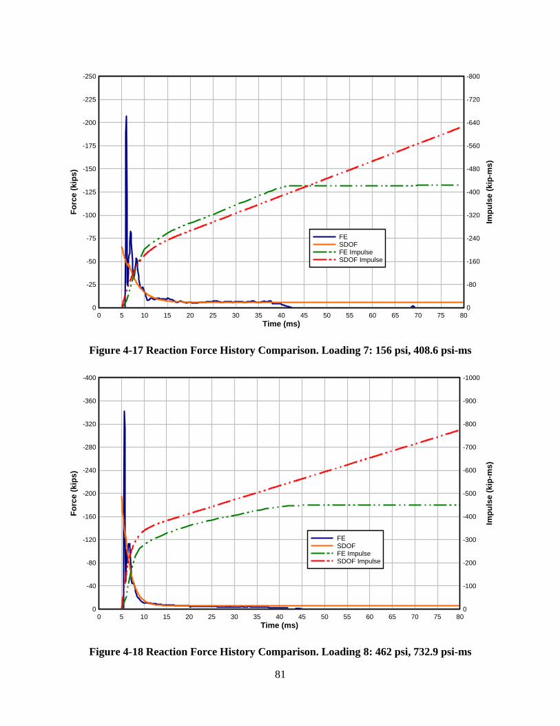
81
Figure 4-17 Reaction Force History Comparison. Loading 7: 156 psi, 408.6 psi-ms
Figure 4-18 Reaction Force History Comparison. Loading 8: 462 psi, 732.9 psi-ms
Time (ms)
Fo
rce (
kip
s)
Imp
uls
e (
kip
-ms)
0 5 10 15 20 25 30 35 40 45 50 55 60 65 70 75 800 0
-25 -80
-50 -160
-75 -240
-100 -320
-125 -400
-150 -480
-175 -560
-200 -640
-225 -720
-250 -800
FESDOFFE ImpulseSDOF Impulse
Time (ms)
Fo
rce (
kip
s)
Imp
uls
e (
kip
-ms)
0 5 10 15 20 25 30 35 40 45 50 55 60 65 70 75 800 0
-40 -100
-80 -200
-120 -300
-160 -400
-200 -500
-240 -600
-280 -700
-320 -800
-360 -900
-400 -1000
FESDOFFE ImpulseSDOF Impulse

82
The duration of the reaction history plateaus are slightly different for the two analysis
methods. This is because FE captures nonlinear material behavior of the concrete better. The
SDOF analysis assumes a constant effective moment of inertia to idealize the effect of cracking
behavior for the entire response whereas FE analysis directly simulates the flexural cracking of
concrete. Similarly, the amount of time that the positive reactions is sustained is different for the
two analysis methods. Again, this is due to the assumption SDOF methodology makes about the
concrete cracked moment of inertia. FE calculations are based on energy, and when the concrete
elements in the model crack, energy is lost. Because there is less energy in the system, the system
has less strain energy stored in the beam at its maximum deflection, so it rebounds slower. The
SDOF analysis does not take this into account and for this reason, it rebounds quicker.
The peak forces in the early stages of response, as discussed previously, are not accurately
predicted by SDOF methodology, but the average forces are accurately predicted. The slight
differences in the duration of the positive phase of the reaction force may be considered to be
negligible. Overall, the SDOF methodology for calculating the reaction force history is acceptable
when compared to FE analysis as long as the extremely short (<1 ms) durations of the peak forces
do not have a significant influence on the connection’s later capacity to resist the more sustained
reaction forces. However, because the SDOF methodology does not capture the force variance or
the peak values, it cannot be considered to be precise.
Others have stated that SDOF dynamic reaction methodology is sufficient for one-way
systems (Morison 2006); the research outlined in this section serves to validate this. The SDOF
methods have generally been proven to be produce accurate results for simply-supported spans, so
it is expected that SDOF methods produce accurate results for other support conditions as well.
Morrison (2006) has stated that SDOF dynamic reaction methodology works for all other support

83
conditions, and they are expected to behave similarly like the general behavior seen in the figures
here for simply-supported spans.
The SDOF methodology is a great analysis tool for predicting dynamic reaction forces
despite not capturing the higher modes of vibration that FE methods provide.
4.4 Comparison of AFRL Connection Demand Test Data to SDOF Reaction Prediction
In the previous section, it was found that SDOF results, when compared to FE results,
produce accurate reaction force histories when only considering the first mode of vibration. SDOF
methods accurately predict the average magnitude of the sustained forces, but does not calculate
the peak reaction force with consistent accuracy. In fact, it tends to under predict the peak reaction
force. In this section, SDOF results will be compared to the full-scale results.
The Air Force Research Laboratory conducted two blast experiments on single-span
concrete sandwich wall panels to examine standard wall construction details without traditional
panel-to-structure embeds (Naito et al. 2011). One goal of the study was to determine if the reaction
demands are comparable to dynamic analysis predictions. Their experiment fit single-span and
multi-span precast and, in some cases, prestressed concrete insulated sandwich panels with load
cells. The test range is shown in Figure 4-19.

84
Figure 4-19 Test Set Up for Full-scale dynamic tests with single span reaction structure
(left) and multi-span reaction structure (right)
The scope of work does not include the multi-span panels and the prestressed single-span
panels, so they will not be analyzed with the FE and SDOF analysis tools available. The wall
panels labeled M3 and M4 are the only wall panels that are simply-supported and are constructed
with conventional reinforcement methods (not prestressed). The elevation and plan views of panels
M3 and M4 are shown in Figure 4-20, Figure 4-21 and Figure 4-22. The panel details are shown
in Table 4-4.

85
Figure 4-20 Single Span TCA Blast Specimens (Naito et al. 2011)
Figure 4-21 Specimen M3 Details (Naito et al. 2011)

86
Figure 4-22 Specimen M4 Details (Naito et al. 2011)
Table 4-4 AFRL Test Sandwich Panel Details
The SDOF analysis was performed by assuming that the panel acts as a fully composite
section. Because panels M3 and M4 are between the pressure sensors 2 and 3, the average peak
Sandwich Panel Details M3 M4
Span (in) 144 144
Width (in) 59 59
Slab Thickness (in) 8 11
Concrete Compressive Strength (psi) 4000 4000
Concrete Density (pcf) 145 145
Reinforcement Spacing (in) 14 14
Longitudinal Rebar Size #4 #4
Longitudinal Rebar Area (si) 0.2 0.2
Transverse Rebar Size #3 #3
Transverse Rebar Area (si) 0.11 0.11
Reinfocement Grade 60 60
Inbound Reinforcement Cover (in) 1.5 3
Rebound Reinforcement Cover (in) 1.5 1.5
Exterior wythe thickness (in) 3 3
Middle wythe thickness (in) 2 2
Interior wythe thickness (in) 3 6

87
pressure and impulse will be considered for the analyses. The instrumentation setup is presented
in Figure 4-23. This figure shows that only reaction force data from load cells 5, 6, 7, and 8 should
be used as panels M1 and M2 are not to be considered due to the prestressing.
Figure 4-23 Instrumentation Single-Span Panels (Naito et al. 2011)
Figure 4-24 and Figure 4-25 show the wall and connection setup. The panels act as partially
fixed-simple, one-way, flexural elements. To obtain the total reaction force, the reaction forces
from the load cells are summed before comparing the measured reaction forces to the reaction
forces that SDOF methodology predicts. When one load cell fails to record meaningful data, the
other load cell will be doubled to come up with an equivalent reaction. The bottom of each panelis
attached to the supporting structure with a base restraint angle and bears against the bottom slab
of the supporting structure while sitting on the concrete grade slab. This can be seen in detail in
Figure 4-24. It was intended to be simply-supported, but forensic analysis showed that it may have

88
behaved more like a fixed connection at the panel’s base. The dynamic reaction equation for a one-
way, fixed-simple support setup is calculated slightly differently than a simply-supported case.
The equations would ultimately reduce the amount of force at the simple end, which is the end
with the load cells. The Biggs dynamic reaction equations for a fixed-simple support setup is
shown in Equation 4-1 and 4-2.
0.26 0.12sV R F (4-1)
0.43 0.19fV R F (4-2)
where Vs is the dynamic reaction at the simply supported end, Vf is the dynamic reaction at the
fixed end, R is the flexural resistance, and F is the applied force. In addition, the equations for the
equivalent static reaction change as well.
Figure 4-24 Single-Span Wall Setup (Naito et al. 2011)

89
Figure 4-25 Single-Span Top Connection Detail (Naito et al. 2011)
The fixed-simple support condition is compared to the simple-simple support condition.
The comparisons are shown in Figure 4-26 and Figure 4-27. The fixed-simple support condition
best represents the measured data because it most accurately predicts the peak force in Figure 4-26,
and in Figure 4-27, it best predicts the sustained reactions and when the reaction forces begin to
dissipate. The parapet was not considered. AFRL engineers observed that the parapet did not have
a significant effect on the response nor the reaction forces. Including the parapet into an SDOF
analysis, would increase the reaction forces before the a higher total applied loading and reducing
the duration of the resistance controlled reaction response when the positive pressure phase exists;
meaning shorter duration inbound reactions but not increasing the total capacity of the panel. This
means it has no total effect on the sustained reaction forces.
In summary, the measured reaction force data from each panel is compared to a SDOF
analysis that uses strength increase factors, and the support setup as simple-fixed. The only way to
make the analysis more accurate is if the measured reflected pressure data is input directly into the
SDOF analysis. This will not be done to better simulate a design scenario. Tension membrane
action can cause much higher forces in the connections. There is no evidence of tension membrane
behavior occurred in the tests because the support conditions did not restrict translation of the ends
of the panel in the longitudinal direction.

90
Figure 4-26 Variable Input Comparisons of Panel M3 reaction force data first 20 ms of response
Time (ms)
Reacti
on
Fo
rce (
kip
s)
20 22 24 26 28 30 32 34 36 38 400
-10
-20
-30
-40
-50
-60
-70
Total Support Reaction ForceSDOF Reaction ForceSDOF Reaction Force with DIFESR M3 with DIFESR M3 without DIFSDOF Reaction Force Simple End of Fixed-Simple AnalysisESR M3 Simple End of Fixed-Simple Analysis

91
Figure 4-27 Variable Input Comparisons of Panel M3 reaction force data full response
Time (ms)
Reacti
on
Fo
rce (
kip
s)
0 20 40 60 80 100 12020
0
-20
-40
-60
-80
Total Support Reaction ForceSDOF Reaction ForceSDOF Reaction Force with DIFESR M3 with DIFESR M3 without DIFSDOF Reaction Force Simple End of Fixed-Simple AnalysisESR M3 Simple End of Fixed-Simple Analysis

92
The measured reflected pressures for test 1 and test 2 are shown in Figure 4-28 and Figure
4-31, respectively. These figures show the measured reflected pressures at each of the three sensors
and show the accompanying impulse. The peak pressure and maximum impulse from these figures
are tabulated in Table 4-4. The blast pressure wave impacts the wall 21 ms after the recording
begins for the first test and 14 ms after the recording starts for the second test. It can be observed
in Figure 4-29 and Figure 4-30 that the first recorded reactions occur 21 ms after recording begins.
The same may be observed for test 2 in Figure 4-32 and Figure 4-33. It can also be determined
from the reflected pressure data that there is an uneven pressure distribution on the wall. As
discussed previously, the average peak pressure and impulse measured from the reflected pressure
sensors are used to perform the SDOF analyses.
The SDOF reaction force histories do not align precisely with the measured total support
reaction force during time where the peak reaction forces occur. The calculated peak forces are
within 20% of the peak forces measured by the load cells. Unlike the comparisons with FE
analyses, higher modes of vibration are not revealed in the measured reaction force data like they
were in Section 4.3.
Semblances of a sustained reaction force may be observed in Figure 4-29 and Figure 4-32.
However, unlike the SDOF analysis, the panel does not maintain a perfectly bilinear resistance
function as the panel deflects. In Figure 4-32, for example, 20 ms into the response (at Time = 35
ms) the measured forces exceed the sustained reaction force that SDOF methods predicted by
100%. In terms of the total response, the measured reaction forces did not resemble the typical
dynamic reaction force history that Keenan outlines in Figure 2-20. The peak reaction forces are
sustained for longer than either Keenan or SDOF analysis predicts with standard SDOF dynamic
reaction equations, and the sustained reaction force that is typical in the Keenan or SDOF reaction

93
force history either is more sporadic and less pronounced (e.g. Figure 4-29 and Figure 4-32), or
does not exist at all (e.g. Figure 4-30 and Figure 4-33). This is due to a nonlinear resistance versus
deflection curve and the excitement of higher mode of vibration.
In test 1, both panels M3 and M4 have fully rebounded by 75 ms into the data recordings.
At this time, Figure 4-29 indicates the beginnings of positive (outbound) reaction forces as does
Figure 4-30. Unlike panel M3, shown in Figure 4-29, panel M4 exhibits a significant decrease in
the reaction force 35 ms into the recording and shows positive reaction forces during this time.
This is very unusual because at this time, the panel is near its point of maximum deflection, which
would suggest that the reaction forces should be in the negative (inbound) direction. This behavior
in panel M4 is observed again in Figure 4-33. No conclusion could be made on why this is
happening, although there are hypotheses. It is suspected that this is due to higher modes of
vibration in conjunction with a large decrease in flexural resistance during the unusual behavior’s
duration. Load cell 8 failed to recording meaningful data in test 1, so it could be suggested that
errors in the data recording from load cell 7 could be amplified when the data was doubled to
represent the total measured reaction force. This type of error is ruled out error because working
load cells in test 2, capture similar results (Figure 4-33). It is common for rebound reaction forces
at the support to damage the connections the most or even cause the connections to fail. This was
observed in multi-span panel tests at the AFRL blast range in 2013 and again in 2014.
.

94
Figure 4-28 Measured Reflected Pressures and Calculated Impulses, Test 1

95
Figure 4-29 Reaction Force History Comparison of SDOF Methodology and Measured Reaction Force Data for Precast Wall
Panel M3, Test 1
Time (ms)
Reacti
on
Fo
rce (
kip
s)
Imp
uls
e (
kip
-ms)
0 20 40 60 80 100 120 140 160 18020 250
0 0
-20 -250
-40 -500
-60 -750
-80 -1000
Total Support Reaction ForceSDOF Reaction Force Simple End of Fixed-Simple AnalysisEquivalent Static Reaction for Simple EndTotal Support Reaction ImpulseSDOF Reaction Impulse

96
Figure 4-30 Reaction Force History Comparison of SDOF Methodology and Measured Reaction Force Data for Precast Wall
Panel M4, Test 1
Time (ms)
Reacti
on
Fo
rce (
kip
s)
Imp
uls
e (
kip
-ms)
0 20 40 60 80 100 120 140 16020 250
0 0
-20 -250
-40 -500
-60 -750
-80 -1000
Total Support Reaction ForceSDOF Reaction Force Simple End of Fixed-Simple AnalysisEquivalent Static Reaction for Simple EndTotal Support Reaction ImpulseSDOF Reaction Impulse

97
Figure 4-31 Measured Reflected Pressures and Calculated Impulses, Test 2

98
Figure 4-32 Reaction Force History Comparison of SDOF Methodology and Measured Reaction Force Data for Precast Wall
Panel M3, Test 2
Time (ms)
Reacti
on
Fo
rce (
kip
s)
Imp
uls
e (
kip
-ms)
0 20 40 60 80 100 120 140 160 18020 200
0 0
-20 -200
-40 -400
-60 -600
-80 -800
-100 -1000
Total Support Reaction ForceSDOF Reaction Force Simple End of Fixed-Simple AnalysisEquivalent Static Reaction for Simple EndTotal Support Reaction ImpulseSDOF Reaction Impulse

99
Figure 4-33 Reaction Force History Comparison of SDOF Methodology and Measured Reaction Force Data for Precast Wall
Panel M4, Test 2
Time (ms)
Reacti
on
Fo
rce (
kip
s)
Imp
uls
e (
kip
-ms)
0 20 40 60 80 100 120 140 160 18020 250
0 0
-20 -250
-40 -500
-60 -750
-80 -1000
Total Support Reaction ForceSDOF Reaction Force Simple End of Fixed-Simple AnalysisEquivalent Static Reaction for Simple EndTotal Support Reaction ImpulseSDOF Reaction Impulse

100
For these tests, the concrete static and dynamic strength increase factors of 1.1 and 1.19
were used, respectively, based on the recommendations from the PDC TR 06-01. In addition, based
on recommendations, the steel static and dynamic strength increase factors of 1.1 and 1.17 were
used, respectively. The strength increase factors applied to the steel reinforcement increase the
flexural resistance of the panel which increases the dynamic reaction forces.
It is possible that there are numerous sources of error within the AFRL open air blast test.
Several things must work correctly for any data, good or bad, to be captured. Explosives are
dangerous, and it is possible that the equipment was damaged when the explosives detonated. The
reflected pressure sensors captured good reflected pressure data. This is known because the shape
the reflected pressure data very closely resembles a typical reflected pressure plot that can be seen
in Figure 2-2. As discussed previously, one load cell, #8 of test 1 (Panel M4), failed to capture any
data at all. As was seen in the FE results, the peak reaction forces last for only milliseconds, so it
is very difficult to capture these peaks with the load cells if they occur at all. Computer analyses
show that when the peak loads occur, they only appear for fractions of milliseconds and then
immediately plummet. It can be seen that the peak pressure lasts milliseconds as well. Since the
dynamic reaction force is directly related to the applied force, the peak dynamic reaction can be
very difficult to measure.
The shape of the reflected pressure history is tied directly to the dynamic reaction force
history, so any simplification of the SDOF input would cause immediate decrease in accuracy of
the dynamic reaction force history. The negative pressure region would directly affect the dynamic
reaction force and would reduce demand over the area where the dynamic reaction force history
plateaus. The equivalent reaction force is meant to resist the forces that are sustained during the
plateau region of the dynamic reaction force history, so if the plateau is less important than

101
originally assumed, the equivalent reaction force is less apt to be the parameter around which
precast wall panel connections are designed.
The limitations of SDOF methodology’s calculation of the dynamic reaction forces is
apparent from Figure 4-29, Figure 4-30, Figure 4-32, and Figure 4-33. Overall, the SDOF
methodology for calculating the dynamic reaction forces is limited in predicting the dynamic
reaction forces. SDOF methodology for calculating the dynamic reaction forces does not predict
the peak reaction forces precisely. Furthermore, SDOF methodology is limited due to assumptions
and simplifications it commonly makes. Assumptions that mispredict dynamic reaction forces
include the use of the static deflected shape as the inertia force distribution in the dynamic reaction
equation, the bilinear resistance function, and an idealized triangular blast pressure curve. Also,
due to the nature of the SDOF methodology, capturing multimodal behavior is not possible.
4.5 Limitations of Connection Design Based on the Flexural Resistance
Typically, the equivalent static reaction is used to determine the force demand for precast
wall panel connections (Oswald and Bazan 2014). The equivalent static reaction is entirely
dependent upon the flexural strength of the panel. The panel’s flexural strength is typically
determined by transportation loads or by the blast loading’s peak pressure and impulse if it is
designed for the blast response criteria. If the panel’s flexural strength is designed for the blast
response criteria, then the panel’s connections are indirectly designed for the blast loading. From
a mechanics standpoint, Equation 2-8 shows that the support forces are dependent on two functions
simultaneously: 1) the flexural resistance and 2) the applied force. Design based on the equivalent
static reaction reduces this to one variable: the maximum flexural resistance.
Figures 4-29, 4-30, 4-32, and 4-33 illustrate that the equivalent static reaction is exceeded
by at least 100% on average for at least 10 ms by the measured reaction forces, and by at least 5

102
ms for the SDOF calculated dynamic reaction forces. As seen from Figure 4-24, the panel
connections for the AFRL blast tests were allowed to bear on the concrete slab at the bottom and
the panel attached to a heavy connection to the restrained load cell at the top. These connections
were not designed for the equivalent static reaction, so they cannot be used to determine the
effectiveness of the current precast connection design methodology. In the blast scenarios defined
by the two AFRL tests, connections designed for the equivalent static reaction would have to
provide addition strength beyond what they are designed for during the 10 ms that the forces
exceed their intended capacity. Dynamic strength increases in the connections due to strain rate
effects could provide the required additional strength, but the reliability of this is unknown. Also,
resistance factors associated variation in component strength hide potential additional strength that
connections may contain.
Table 4-5 compares the equivalent static reaction force to the peak forces found in the FE
and SDOF analyses. The data from this table are combined to produce Figure 4-34. It can be seen
from this figure that the equivalent static maximum shear exceeds the peak force predicted by
SDOF analysis for support rotations under 1° of support rotation. The data from FE analysis
suggests that for the smallest blasts tested, the peak reaction will exceed the equivalent static
reaction by at least 440%. As the support rotation and level of damage increases, the amount the
peak reaction force exceeds the ESR increases. SDOF analyses show that support rotations below
4°, the peak reaction force does not exceed the ESR by more than 150%.

103
Table 4-5 Comparison of Equivalent Static Reaction to Peak Reactions
Figure 4-34 Peak Reaction Exceedance of ESR at Varying Levels of Support Rotation
Designing connections based on the short duration peak forces illustrated by the FE
analyses in Section 4.3 is not economical. The peak pressures and impulses were chosen to
represent actual design scenarios, and the reaction forces calculated by these analyses show that
the forces can reach as high as 150 kips. Designing the connections for reaction forces so high
would not be feasible nor practical. Rather than designing the connections for the FE peak
reactions, consider the possibility of designing the connections for the SDOF dynamic reactions.
Loading
Support
Rotation
(degrees)
DYNA Peak Reaction (kips) % Peak Exceeds ESMS SBEDS Peak Reaction (kips) % Peak Exceeds ESMS
1 0.25 47.9 441.2% 7.76 -12.3%
2 1.45 82 826.4% 12.182 37.6%
3 3.05 111 1154.1% 20.194 128.2%
4 2.99 97.3 999.3% 15.625 76.5%
5 6.24 148 1572.1% 31.044 250.7%
6 8.74 165 1764.2% 38.445 334.4%
7 13.66 207 2238.7% 65.953 645.1%
8 38.4 342 3764.0% 104.922 1085.4%
*Equivalent Static Maxmimum Shear (ESMS) = 8.85 kips
Support Rotation (degrees)
% P
eak R
eacti
on
Exceed
s E
qu
ivale
nt
Sta
tic R
eacti
on
0 5 10 15 20 25 30 35 40-500%
0
500%
1000%
1500%
2000%
2500%
3000%
3500%
4000%
FE Analysis Peak Force Exceedance PercentageSDOF Analysis Peak Force Exceedance Percentage

104
As was shown in Section 4.3, the SDOF dynamic reactions accurately predict the average of the
FE results, and in Section 4.4 the SDOF dynamic reaction predict the peak forces measured in full
scale tests typically within 20%. In addition to generally predicting the peak forces, SDOF analyses
also reliably predict the sustained reaction forces (given the panel has a bilinear resistance curve).
It is of the utmost importance that at least panels with moderate levels of damage have
connections capable of carrying the load demand. The objective of the engineer is to design
connections that will survive, but in cases where the panel fails and debris is launched from the
panels, the safety of a building’s occupants is not controlled with stronger connections. It is also
more important that they have the strongest connections so they can dissipate the most energy
through panel failure. As the panel deforms, it dissipates great amounts of energy. The connections
must be strong enough for the panel to be able to achieve the desired energy dissipation. If the
connections fail before the panel fails, then a great amount of blast energy dissipation potential is
lost.
Because there is the capability to produce accurate dynamic reaction results quickly and
easily with SDOF methods, they should be considered when designing connections. The
equivalent static reaction for the panel used to compare SDOF to FE analyses in Section 4.2 and
described in Chapter 3 is roughly 8 kips. This means the design force is less than the peak force,
but exceeds the force demand for the other majority of the time. This may be an adequate design
as long as the strain rate effects of the connection provide enough additional strength for the short
duration peak loads. Short duration loads in combination with strain rate effects make connection
design much harder. However, just because they are not understood means that they should be
ignored entirely. It can be seen from Figure 4-13, for example, that the peak loads last for only a
few milliseconds and the other semi-sustained reaction forces last longer. A connection designed

105
for the maximum equivalent static shear may inherently have the additional strength due to strain
rate effects needed to resist the short duration peak loads.
Ultimately, the connection must retain enough strength and ductility to survive the entirety
of the blast. This includes the inbound reaction forces after the peak loads as well as the rebound
reaction forces. If the connection is damaged too heavily due to the short duration peak reaction
forces, it may not achieve the required ductility and increase chance of failing during rebound.
Also, it is implied that the supports are expected to be able to rotate. For the panel to achieve its
maximum ductility (and therefore dissipate the most energy), it must be allowed to deflect fully.
Unfortunately, this creates a scenario where the connection design is complex. Designing
connections based on the equivalent static force is certainly the simplest and most economical, and
has been shown to be sufficient in 90% of tests as was discussed in section 2.8.7 (Oswald and
Bazan 2013). The test data found in this report shows that the equivalent static reaction is regularly
exceeded by peak reaction forces, but if tests by top researchers in the structural engineering blast
field show that the equivalent static reaction force is sufficient for connections without bias, then
there is not enough evidence in this report to refute that. Still, it is recommended that the
connections are tested further, because ideally, no connection should fail under expected loads.

106
Chapter 5. Conclusions and Recommendations for Future
Work
A comprehensive understanding of the mechanics involved in the reaction force variation
through time for precast concrete panels subjected to blast loads was developed through an
exhaustive literature study, comparisons made between SDOF and FE analyses and by observing
load cell data from tests carried out. It was found that the dynamic reaction force is a function of
the resistance, the applied force, and the inertia force distribution at any point in time. Analyses
suggest a near instantaneous peak force followed by a period of sustained reaction force until the
panel has fully rebounded provided the resistance of the beam is bilinear. The dynamic reaction
force history may be found at any point in time if the applied force, resistance of the beam, and
the general shape of the inertia force distribution is known. Because the first mode of vibration
dominates the response, the deflected shape of a statically loaded beam may be used to
approximate the inertia force distribution, but errors are expected. Measured reaction force data
did not perfectly align with the analyses reaction forces due to making assumptions and
simplifications. The assumptions and simplifications include not fully accounting for strain rate
effects, idealizing the applied forcing function as a triangular pressure curve with a peak pressure
and equivalent impulse, idealizing the support setup at fixed-simple when it is actually between
simple-simple and fixed-simple, excluding the possibility for tension membrane effects and
excluded the blast pressure on the parapet. Also, SDOF cannot account for modes beyond the first
mode of vibration.
SDOF analyses were performed and compared to FE analyses and measure load cell data
from full-scale blast tests to evaluate the accuracy and limitations of the SDOF methodology for
predicting connection demand. The SDOF and FE analyses produce very similar results for mid-
range blast loads that do not induce heavy damage or very little damage if the effects of higher

107
modes are ignored. Higher modes of vibration amplify reaction forces greatly, but for short periods
of time (1ms). The study shows that the general magnitudes and shapes of the reaction force
histories are very similar for loads that the panel is expected to be designed for. In this sense, it
may be concluded that SDOF dynamic reaction prediction methodology is accurate. By developing
an understanding of the mechanics involved in dynamic reaction forces, it becomes apparent that
the limitations for the SDOF methodology are directly related to the assumptions made. The
combined effect of simplifying the loading, support conditions, strain rate effects, mode of
vibration, and ignoring tension membrane effects and area outside the span of the panel limit the
accuracy of SDOF methodology for predicting the dynamic reaction forces.
It is still unknown what the limitations are for using the static flexural strength as the basis
for connection design. Designing connections for the equivalent static reaction force, which is
based on the static flexural strength of the panel, is unsettling because it relies on the strength of
the connections to increase due to strain rate effects. The numerous dynamic reaction force
histories from analyses indicate that the pseudo-sustained reaction force will be roughly 78% of
the equivalent static reaction force. This provides a reasonable factor of safety during this portion
of the dynamic reaction force history. However, initial reaction forces, which typically last shorter
than 20 milliseconds, and the peak reaction force, which typically lasts for a few milliseconds,
greatly exceed the equivalent static reaction force. For the connection to persist and retain enough
strength to support the weight of the wall, the connection must be able to resist the peak forces.
Because the peak forces have such a short duration, and strength increases due to strength increases
can increase the capacity of the connection when the peak forces occur, the connections designed
for the equivalent static reaction maintain a high percent chance of survival. In addition, tests show
that most precast wall connections subjected to blast designed for the equivalent static reaction

108
force are able to resist the reaction forces imparted to them. Therefore, it is not the recommendation
of this thesis to halt the practice of designing connections for the equivalent static reaction force;
however, it is urged that the connections are properly fabricated and prepared to either eliminate
tension membrane response altogether, or be able to resist the forces associated with tension
membrane response if connection failure is most commonly due to these effects.
Recommendation for future work:
o Testing of the static capacity of connections and the dynamic capacity of the
connections in typical failure modes associated with connection failure in blast
scenarios
o Investigate the strain rates and the dynamic strength increase factors associated with
precast wall panel connections subjected to blast loadings
o Investigate the effect of tension membrane response on the reaction forces.

109
References
ABS Consulting Ltd. 2006. Design, materials and connections for blast-loaded structures.
Research Report 405, Warrington, UK: Health and Safety Executive.
ACI Committee 318. 2011. Building Code Requirements for Structural Concrete (ACI 318-11)
and Commentary. Farmington Hills, MI: American Concrete Institute.
Adaros, MS, S Wood, and PV Eepoel. 2013. Effect of Inertia Forces on Support Reactions of
Beams subjected to Uniform Blast Loads. Boston, MA: SEI Structures Congress.
Andersson, Sebastian, and Hampus Karlsson. 2012. Structural Response of Reinforced Concrete
Beams Subjected to Explosions. Master's Thesis, Goteborg, Sweden: Chalmers University
of Technology.
Ardila-Giraldo, Oscar A. 2010. Investigation on the Initial Response of Beams to Blast and Fluid
Impact. PhD Dissertation, Purdue University.
ASCE. 2010. Design of Blast-Resistant Buildings in Petrochemical Facilities. Reston, VA:
ASCE.
ASCE/ SEI. 2010. Standard 7-10: Minimum Design Loads for Buildings and Other Structures.
Reston, Virginia: American Society of Civil Engineers.
Biggs, John M. 1964. Introduction to Structural Dynamics. New York, NY: McGraw-Hill.
Billeck, A, and S Marjanishvili. 2011. "The Evaluation of Pre-stressed Pre-cast Panels Subjected
to Blast." Structures Congress 1337-1346.
Chopra, A. K. 2012. Dynamics of Structures, 4th Ed. Upper Saddle River, New Jersey: Prentice
Hall.
Dayton Superior Corportation. 2014. COREWALL® STRAP TYPE SLOTTED INSERT,
COREWALL® STRAP ANCHOR, COREWALL® SLOTTED STRAP ANCHOR AND
COREWALL® THREADED STRAP. Accessed December 2, 2014.
http://www.daytonsuperior.com/Lists/Product%20Catalog1/product.aspx?List=3c62f7a2-
1783-4ee6-a0c4-2642507b1472&ID=265.
Department of Defense Protective Design Center. 2008. "United Facilities Criteria 3-340-02:
Sructures to Resist the Effects of Accidental Explosions."
Feldman, A., and C. P. Siess. 1958. Investigation of Resistance and Behavior of Reinforced
Concrete Members Subjected to Dynamic Loading Part II. Technical Report, Urbana-
Champaign: University of Illinois.
Gibson, Phillip W. 1994. Blast Overpressure and Survivability Calculations for Various Sizes of
Explosive Charges. Survivability Directorate Technical Report, Natick, MA: U.S. Army
Natick Research, Development, and Engineering Center.
Halfen USA. 2014. HALFEN HTA Cast-In Channels. Accessed December 2, 2014.
http://www.halfenusa.com/.

110
Keenan, William A. 1965. Dynamic Shear Strength of Reinforced Concrete Beams Part I.
Technical Report, Port Hueneme, California: U.S. Naval Engineering Laboratory.
Keenan, William A. 1976. "Shear Stress in One-way Slabs subjected to Blast Load." Minutes of
the Explosive Safety Seminar 533-568.
Krauthammer T., Shahriar S., and Shanaa H. M. 1990. "Response of Reinforced Concrete
Elements to Severe Impulsive Loads." Journal of Structural Engineering 1061-1079.
Krauthammer, T. 1999. "Blast-resistant sturctural concrete and steel connections." International
Journal of Impact Engineering 887-910.
Krauthammer, T., and S. Shahriar. 1988. A Computational Method For Evaluating Modular
Prefabricated Structural Element For Rapid Construction of Facilities, Barriers, and
Revetments to Resist Modern Conventional Weapon Effects. Technical Report, Tyndall
Air Force Base, Florida: Air Force Engineering and Services Laboratory.
Logan, Daryl L. 2007. A First Course in the Finite Element Method. Toronto: Thomson Canada
Limited.
Lowak, Michael J., and John R. Montoya. 2012. Shock Tube Testing of Pre-Cast Concrete
Panels. Technical Report, San Antonio, TX: Baker Engineering and Risk Consultants
Inc.
LSTC. 2011. LS-Dyna. Accessed October 28, 2014. http://www.lstc.com/products/ls-dyna.
Magnusson, Johan. 2007. Structural Concrete Elements Subjected to Air Blast Loading. PhD
Licentiate Thesis, Stockholm, Sweden: KTH Royal Institute of Technology.
Magnusson, Johan, Mikael Hallgren, and Anders Ansell. 2014. "Shear in Concrete Structures
Subjected to Dynamic Loads." Ernst & Sohn Publishing House for Architecture and
Technical Sciences GmbH & Co. 55-65.
Malvar, L. J., and C. A. Ross. 1998. "Review of Strain Rate Effects for Concrete in Tension."
ACI Materials Journal 735-739.
Malvar, L. J., J. E. Crawford, J. W. Wesevich, and D. Simons. 1997. "A Plasticity Concrete
Material Model for DYNA3D." International Journal of Impact Engineering 847-873.
Malvar, L. Javier, and John E. Crawford. 1998a. "Dynamic Increase Factors for Concrete."
Twenty-Eighth DDESB Seminar. Orlando, FL.
—. 1998b. "Dynamic Increase Factors for Steel Reinforcing Bars." Twenty-Eigth DDESB
Seminar. Orlando, FL.
Morison, Colin M. 2006. "Dynamic response of walls and slabs by single-degree-of-freedom
analysis-a critical review and revision." International Journal of Impact Engineering
1214-1247.
Naito, Clay, Mark Beacraft, John Hoemann, Jonathon Shull, Bryan Bewick, and Michael
Hammons. 2011. Dynamic Performance of Insulated Concrete Sandwich Panels Subject
to External Explosions. Technical Report, Tyndall AFB, FL: Air Force Research
Laboratory.

111
Newberry, Charles Michael. 2011. Finite Element Simulation and Assessment of Single-Degree-
of-Freedom Prediction Methodology for Insulated Concrete Sandwich Panels Subjected
to Blast Loads. Master's Thesis, Auburn, AL: Auburn Univeristy.
Newmark, N. W. 1953. "An Engineering Approach to Blast Resistant Design." Proceedings of
ASCE.
Nickerson, Joseph, Anthony Consunji, and James Davidson. 2014. Finite Element Simulation of
Precast/Prestressed Insultated Sandwich Panels Optimized for Construction of
Government Facilities. Research Fellowship Report, Auburn, AL: Auburn University.
Oswald, C J, and D C Morgan. 2009. Case Study of Blast Design for Precast Panels on a Large
Office Building. Conference Paper, San Antonio, Texas: Protection Engineering
Consultants.
Oswald, Charles J, and Marlon Bazan. 2013. Literature Search Report for Optimization of
Concrete Panels For Blast Design with Proposed Full-Scale Testing. Technical Report,
San Antonio, TX: Protection Engineering Consultants.
Oswald, Charles J, and Marlon Bazan. 2014. Performance and Blast Design for Non-Load
Bearing Precast Concrete Panels. Structures Congress, San Antonio, TX: Protection
Engineering Consultants.
PCI. 2004. PCI Design Handbook for Precast and Prestressed Concrete, 6th Edition. Chicago:
PCI MNL 120-04.
PCI. 1997. "State-of-the-Art of Precast/Prestressed Sandwich Wall Panels." Journal of the
Precast/Prestressed Concrete Institute (Journal of the Precast/Prestressed Concrete
Institute) 42.
Ross, Timothy. 1983. Direct Shear Failure in Reinforced Concrete Beams under Impulsive
Loading. Technical Report, Kirtland Air Force Base, NM: Air Force Weapons
Laboratory.
Ross, Timothy J, and Helmut Krawinkler. 1985. "Impulsive Direct Shear Failure in RC Slabs."
American Society of Civil Engineers Journal of Structural Engineering (ASCE) 1661-
1677.
Tedesco, JW, WG McDougal, and CA Ross. 1999. Structural Dynamics: Theory and
Applifcations. California: Addison Wesley Longman.
The Constructor. 2014. Precast Concrete Methods. Accessed 12 2, 2014.
http://theconstructor.org/concrete/precast-concrete-methods-3/422/.
USACE. 2008. Methodology Manual for the Single-Degree-of-Freedom Blast Design Effects
Spreadsheets (SBEDS). Protective Design Center Technical Report 06-01 Rev. 1.

112
Users Guide on Creating SBEDS and LS-DYNA
Keyword Input Files
SBEDS INPUT INTERFACE
SBEDS allows several different options when inputting the structural element’s parameters
and it allows several options for defining the applied loads as well. It offers the option to choose
between different acceptor system types such as one-way corrugated metal panels, reinforced
concrete slabs and different types of masonry. The options are shown in the figure below.
SBEDS Acceptor System Types
After choosing the acceptor system, a customized input interface is created. The interface
and the chosen inputs are shown in the following figure.

113
SBEDS Acceptor System Input Interface
The straightforward inputs will not be discussed at length such as the span length, slab
thickness, reinforcing steel spacing and cover, concrete density, and concrete compressive
strength. The boundary condition chosen was “One-Way: Simple-Simple, Uniformly Loaded,”
and it was chosen because the blast causes a uniformly distributed pressure over the span of the

114
wall panel, the supports are assumed to be simple, and the supports are only located at two opposite
ends of the beam and do not restrict translation at the other edges. It also offers the option to choose
two-way response, different types of boundary conditions such as fixed-simple, fixed-fixed and
cantilever behavior for one-way boundary supports, and three and four sides simply-supported or
fixed-supported for two-way boundary support constraints. The concrete static strength increase
factor (SSIF) adjusts the concrete compressive strength for expected increases in strength beyond
the 28 day compressive strength normally specified (USACE 2008). The concrete dynamic
compressive strength increase factor (CDIF) adjusts to account for increases in strength in the
concrete when the concrete strain rate is high. The strain rates in reinforced concrete components
responding to far-range blast loads are at least 0.10 sec-1 and the strain rates for close-range blast
loads are at least 0.30 sec-1. According to the following figure, these strain rates would correspond
to dynamic increase factors of 1.19 and 1.25 respectively. It is recommended that lower DIF values
for each load range of 1.12 and 1.16, respectively, are used instead (Department of Defense
Protective Design Center 2008).

115
Strain Rate vs. Concrete Ultimate Compressive Strength (USACE 2008)
In order to be consistent with the FE analysis, both the concrete dynamic compressive
strength and the concrete dynamic strength increase factor will be disregarded and set to values of
1. This will cause inaccuracies when comparing the SDOF analysis results to recorded reaction
force data from shock tube and open air tests. Higher strength increase factors increase the ultimate
flexural resistance, and higher flexural resistance causes the dynamic reaction force to increase at
times during the reaction force history.
In the “User Defined” reinforcement section of the SDOF acceptor system input interface
(not pictured), it allows the user to input the reinforcement yield strength, ultimate strength,
average strength increase factor (SIF), and dynamic increase factor (DIF) adjustment. The average
strength increase factor is different from the SSIF. Instead of accounting for how concrete naturally
increases its strength over time, it is a factor that adjusts the DIF for stronger steels. Testing of
high yield strength steels have shown that the DIF decreases with increasing yield strength

116
(USACE 2008). The SIF accounts for this change. The table below is used to determine the SIF
and the DIF for different strength steels.
Material Strength Increase Factors for Structural Steel
In the same line of reasoning for selecting the concrete increase factors disregarded and
simplified to be 1, the steel increase factors will also be disregarded. It is important to keep the FE
analysis model and the SDOF model consistent so they can be more aptly compared. Also, a yield
stress and ultimate stress of 60,000 psi for the steel was chosen to be consistent with the inputs and
to create an elastic-perfectly-plastic stress scenario for simplicity to create a bilinear resistance-
deflection curve. The bilinear resistance curve created from these inputs is shown in the figure
below.

117
Bilinear Resistance Curve
0
0.5
1
1.5
2
2.5
3
3.5
4
4.5
0 0.05 0.1 0.15 0.2 0.25 0.3
Re
sis
tan
ce
Deflection
Resistance vs Deflection

118
Blast Parameter Input Interface
When defining the blast parameters, it allows three different blast load input setups: 1)
Manual Input, 2) Charge Weight and Standoff and 3) Pressure-time history file. The manual input
is best when the pressure at certain time steps is known, or a pressure-impulse is known, but the
charge weight and standoff distance is not known. The charge weight and standoff distance is
generally ideal for analysis when the charge weight and standoff distance are known. The pressure-
time history file is best when one SDOF analysis has already been performed for a secondary

119
member, and the analyst wants to use the reaction history from the first SDOF analysis as the input
for the second SDOF analysis.
The charge weight and standoff section of the input interface allow the user to choose a
charge weight in equivalent pounds of TNT (the standard for explosive amount) and the distance.
The user is given the option to choose a blast phase with a positive phase only or a positive and
negative phase. The real blast phase does have a negative component, but it will be neglected for
all analyses. Finally, the charge weight load type must be selected. It provides the options: reflected
with clearing, reflected without clearing and side-on. The reflected without clearing is the
appropriate choice because the wall is assumed to be freestanding in the open without an overhead
clearing and side-on is appropriate when the pressure is not hitting the wall directly, and instead
the pressure is being reflected off of a wall orthogonal to the direction of the blast. The incidence
angle is the angle in degrees from the normal plane of the wall. If the blast is aimed directly at the
wall, it will be 0 degrees/radians. By choosing 0 degrees for the incidence angle, SBEDS will
produce the worst case scenario/ the largest response.
After inputting all of this information, SBEDS is ready to be run. Also, the inputs may be
saved to be retrieved later if wanted.
SBEDS RESULTS AND SDOF OUTPUT
Under the “Results” and “SDOF Output,” the user can access the software’s most important
results. SBEDS produces many useful results that are used within blast design. Most importantly,
it provides the maximum support rotation and ductility ratio. These results are used to approximate
the level of damage the panel is expected to incur upon receiving a blast with the magnitude
specified. In the “Results” tab, SBEDS produces the maximum and minimum deflections and the

120
times that they occur, respectively. It also produces the maximum and minimum resistances and
the times that they occur, respectively. These outputs are shown in the table below.
SBEDS Results Summary
Other useful quantities and figures can be found in the “Results” tab as well. For
instance, the displacement history, applied force history, resistance and equivalent P-delta force
histories, resistance vs. displacement, and dynamic shear history figures can all be found here. In
addition, the peak dynamic reactions and strain rates to yield are tabulated neatly for the user to
access within the Results tab. They are shown in in the table below.
Peak Dynamic Reactions and Strain Rate to Yield
In the “SDOF Output” tab, several different analysis quantities can be found at each
timestep, and can be saved to DPLOT files if so desired. The quantities that can be found here
are time (ms), applied force (psi), equivalent P-delta (psi), deflection (in), velocity (in/ms),
acceleration (in/ms2), stiffness (psi/in), resistance (psi), load-mass factor, axial load (lb/in), and
dynamic reactions for the long and short span (psi). The long span dynamic reaction is the
default dynamic reaction output for one-way slabs, and the short span dynamic reaction outputs
the dynamic reaction in the shorter direction for two-way slabs. It can be noted that SBEDS
calculates the resistance, stiffness, axial load, and the dynamic reactions in force per unit area of
qmax = 0.6 deg.
m 6.26
Xmax = 0.66 in at time = 25.10 msec
Xmin = 0.00 in at time = 0.00 msec
Rmax = 4.13 psi at time = 25.10 msec
Rmin = -4.12 psi at time = 43.60 msec
Results Summary
Vmax,Long = 2.47 psi
Vmax,Short = 0.00 psi
For Steel 0.406 1/ sec
For Concrete 0.392 1/ sec
Strain Rate to Yield*
Peak Dynamic Reactions

121
the panel for one and two-way slabs. This is so that that a typical one-foot section of the slab
may be provided as the input for the analysis to represent a slab for any width. After SBEDS
performs the SDOF analysis, the user may multiply a data point, or a set of data points by the
area of the entire panel being analyzed to obtain the appropriate response information for the
entire panel. For the example outlined at the beginning of the section, the set of long span
dynamic reaction data (in psi) would be multiplied by the clear span length (120”) and the width
(32”) to obtain the dynamic reaction force history for one support of the panel.
LS-DYNA KEYWORD INPUT FILE CREATION
Before creating the input file, it is important to be aware that all inputs are unitless so it is the
responsibility of the analyst to insure that units remain consistent throughout the process. For the
models chosen, everything was done in terms of pounds force, inches, and seconds. Steps to
creating the input file:
1) Mesh the Solid Shape
a) Use ‘Mesh’ on Card 7. This will cause the input box in the next figure to appear.
b) As a preliminary measure: size the solid elements (concrete sections and supports) so that
the cover can be accommodated for the steel reinforcement later.
c) Choose element sizes that are close to uniform for individual elements, and attempt to make
solid elements as close to cubes as possible. Ensure that corner nodes of touching elements
lined up. This research used 2x2x0.75” for outer concrete parts, and 2x2x1” for inner
concrete part.
d) Input the minimum and maximum dimensions in for the x, y, and z directions to define the
size of the part.

122
e) Define the element sizes by selecting the ‘Size’ radio button and then choosing the element
in the Vx, Vy, and Vz boxes. The completed mesh is shown below.
Mesh input box

123
Completed Mesh of the 3 concrete wythes and supports
2) Mesh the Steel Reinforcement
a) Use ‘ElEdit’ on Card 2.
b) Use the ‘Create’ radio button under the “Element” column, and select Beam.
c) Click the starting node for the reinforcement and then the ending node for reinforcement
and then a third node to define its local z-axis. The completed beam mesh is shown above.
d) The elements must be the same size as adjacent nodes so that they can be merged and
exhibit the necessary strain compatibility behavior.
i) Split elements by using the Split/Merge tool in ElEdit. Divide them so that they have
the same division as the solid mesh they are within.

124
ii) Merge duplicate nodes by using ‘Dup Node’ on Card 2 and click ‘Merge Duplicate
Nodes.’ Set the tolerance small enough to ensure the nodes that are supposed to merge
do merge, and so the nodes that are not supposed to merge do not merge.
Completed Mesh of the beam elements
3) Define the Material Properties
a) Use ‘Mat’ on Card 3
b) Create a new material property and assign it a new unique material identification number
(MID)
c) For concrete, the material model used is MAT072R3-CONCRETE_DAMAGE_REL3.
This is the material property model for concrete that simulates the behavior of damaged

125
concrete that crushes or cracks and subsequently loses strength. The compressive strength
and mass density are input here.
Material Input Form for Concrete
d) For steel, the material model used is MAT003-PLASTIC_KINEMATIC. This is a material
property model for a material that is expected to behave elastically until a certain stress,
and then behaving in a perfectly-plastic fashion. The yield stress and the mass density are
input here. This is an idealization for simplification.

126
Material Input Form for Steel
4) Define Section Properties
a) Use ‘Section’ on Card 3
b) The section properties are defined for all beams at once and for all solids at once.
c) Create a new section property and assign it a new unique section identification number
(SECID)
d) For beam elements, the shape of the beam is chosen under CST as 1 for circular, and then
the diameter for the beams are defined here (0.625 for #5 bars).
e) For solid elements, the default element formulation option of 1 causes the solid element to
have constant stress. This is appropriate for the purposes of this research.
5) Assign Material and Section Properties to appropriate Parts
a) Use ‘Part’ on Card 3
b) For each part (the three concrete layers, the two supports and the four steel reinforcement
bars), assign it a unique part identification number (PID) and then assign the appropriate
MID and SECID.
6) Define Contacts

127
a) Create new segment sets that define the area on the two contact surfaces that will contact
each other.
i) This is done by using ‘SetD’ on Card 5
ii) Use the create function for SET_SEGM and then defining the area in the view window.
(1) It will select ALL surfaces within the box, not just the furthest surface forward, so
in order to select only the appropriate surfaces of the elements, the view must be
lined up so that the surface is orthogonal to the view of the user.
(2) If the user must only select a certain part, other parts may be hidden by using the
‘Spart’ tool in the window option button below the viewport.
iii) Click apply to save the segment set
iv) Repeat for all contact surfaces (4: panel bottom, panel top, top support, bottom support)
b) Use ‘Contact’ on Card 3
c) Edit CONTACT_AUTOMATIC_SURFACE_TO_SURFACE. This will automatically
enforce a contact condition between two segments if one segment enters another segments
space
d) Give the contact a new, unique contact identification number (CID)
e) Provide the slave segment set ID and the master segment set ID (from the segment sets
defined earlier). It does not matter which set it slave or master, but they must be the two
segment sets that are expected to come into contact.
f) Accept and hit ‘Done’.

128
Contact Input Form for CONTACT_AUTOMATIC_SURFACE_TO_SURFACE
7) Define Load
a) Create a segment set to define the area that the blast will act over.
i) Refer to step 6a for how to define a segment set
b) Use ‘Define’ on Card 3
c) Edit ‘Curve’ and create a new load curve
d) Enter the blast load steps one at a time. Input time values in A1 (Abscissa values) and
pressure values in O1 (Ordinate values). Click ‘Insert’ after entering each set to add it to
the whole set of data.
e) Click ‘New’ to see a plot and confirm the data entry.
f) ‘Replace’ and ‘Delete’ will delete the highlighted values
8) Setup Controls
a) Use ‘Control’ on Card 3
b) Edit ‘Termination’

129
i) Choose an analysis duration (ENDTIM) that will capture the full behavior until
rebound. This may take iteration. The duration selected for this analysis is 0.080
seconds, or 80 milliseconds.
c) Edit ‘Timestep’
i) Choose an analysis timestep duration. A good rule of thumb is to include at least 20
steps in the analysis. A timestep of 0.003 seconds, or 3 milliseconds, was used.
9) Request additional outputs
a) Use ‘Dbase’ on Card 3
b) The additional output wanted for this analysis is the RCFORC ASCII option.
i) This will output the force applied at the contacts.
ii) This is the connection force output that the analysis was intended to find.
iii) If nodes were setup as the supports, NODFOR ASCII option should be used
c) Edit ‘ASCII_option’
i) Check the box for RCFORC
(1) If it is not already, set the timestep (DT) equal to the timestep designated earlier
(2) Select 1 for Binary so an ASCII file is written to be processed later
10) Save the file as a keyword file (extension .k)
LS-DYNA POST PROCESSING OUTPUT
After all these steps have been completed, the file is ready to be run by LS-DYNA. This
can be done through several methods. A high powered computer cluster, or HPCC, can perform
an analysis using several parallel processors to analyze large files very quickly. If a HPCC is not
available, DYNA will be able to run on a regular desktop computer, provided it has the necessary
processing power. For a model of this size, a single processor is all that is necessary. In addition,

130
if multiple processors are used, the RCFORC ASCII binary output file will not be produced; this
will render the analysis nearly fruitless. The HPCC is accessed through a Linux based secure script
emulation tool SecureCRT. By creating a shell file, LS-PrePost keyword files can be sent to the
LS-DYNA FE analysis tool, and then when the analysis is complete, the d3plot files will be placed
in the network destination the user specifies in the shell file. A sample shell file will be provided
in the appendix. “d3plot” is the output file that LS-PrePost uses to display the output data. The
next section will explore the d3plot in more detail.
There is a tutorial on how to setup SecureCRT for LS-DYNA on Auburn University’s
Engineering Network Services Access Informational website. The user can follow this link
information on how to set up SecureCRT: http://eng.auburn.edu/admin/ens/hpcc/access-
information.html#Set%20up%20SecureCRT. To interact with the HPCC within SecureCRT, the
user must be familiar and be able to use a combination of basic and advanced Linux commands.
A list of commands available and how to use them can be found at the following websites:
Basic Commands: http://eng.auburn.edu/admin/ens/hpcc/basic-commands.html
Advanced Commands: http://eng.auburn.edu/admin/ens/hpcc/advanced-commands.html
This is the shell file sent to SecureCRT to request 1 processor to run the analysis on the Auburn
High Power Computer Cluster.
Additional access information can be found at:
http://eng.auburn.edu/admin/ens/hpcc/access-information.html
#!/bin/sh
#name the program
#PBS -N spp
#PBS -o output_dyna
#default output and error file
#PBS -e error_dyna
#asking for 1 node and 1 processor for 50hrs
#PBS -l nodes=1:ppn=1,walltime=50:00:00

131
#define your directory path This saves the file to this
directory The directory must exist
#PBS -d /home/u3/acc0017/dyna/
#following 2 lines ensures you'll be notified by email when your
job is done
#PBS -M [email protected]
#PBS -m e
#see which host is performing computation
/bin/hostname > output
#print the time stamp if you want
date >> output
#invoke ls-dyna.singlecpu and I=source_file >> your output file
/opt/ls-dyna/ls-dyna.singlecpu I=60ft.k >> output
#print out end time
date >> output
LS-PREPOST POST PROCESSING OUTPUT
The analysis is complete when the analysis has been run to the full duration specified.
While it does not explicitly tell the user that the analysis has been completed, there are some
indicators to alert the user when it has finished. The indicators are:
1) The d3plot file stops increasing in size.
2) An email notification from the computer cluster alerts the user that the analysis has
completed.
3) When the d3plot is opened (it can be opened while the analysis is still ongoing), the user
sees that the total duration matches the duration specified in the control portion of the input
file.
Once the analysis, it complete, the model can be viewed in the viewport from any angle or
preset view (top, bottom, left, right, front, back). The model is loaded into LS-PrePost by selecting
File, Open, LS-DYNA Binary Plot, and then selecting the appropriate file which will most likely

132
be named d3plot. If the file is exceptionally large, then the d3plot file will have additional portions
d3plot01 and d3plot02 and so on and so forth. These will be automatically loaded with the original
d3plot when it is loaded. If there is a residual d3plot from another analysis, this will cause an error.
In addition to visually observing the deflection, relative velocity, and acceleration, several
other quantities can be numerically observed, plotted, and saved into comma separated value
(CSV) files which can be opened in Excel for easy tabulation and further analysis. Nodal
displacement were measured and tabulated by selecting the node which visually displaced the most
and graphing its displacement in one of the main directions through time. In Card 1 in the LS-
PrePost menu, ‘History’ was used to select the nodal “Z-displacement.” This was then plotted by
hitting “Plot” and then saved as a “MSoft CSV(Single X-Axis)” file with an output interval of 1.
This file could then be formatted within Microsoft Excel as needed. To obtain the reaction force
values, the rcforc file must be loaded into LS-PrePost from the folder that the d3plot is in by
clicking load in ‘ASCII’ in Card 1. The appropriate contact segment set would be selected (i.e.
“Sl-1:Bottom Support”), the appropriate force direction would be selected (i.e. “Z-force”), and
‘New’ was clicked to create the plot, which could then be saved and formatted as needed like the
displacement example above.

133
Sample LS-DYNA Keyword File
Note: Some sections that repeating numerical inputs were omitted for the sake of space. A full
word document sample of the keyword file is 585 pages.
$# LS-DYNA Keyword file created by LS-PrePost 3.2 - 10Apr2013(12:00)
$# Created on Aug-13-2014 (16:54:56)
*KEYWORD MEMORY=Dù‚; NCPU=1
*TITLE
$# title
LS-DYNA keyword deck by LS-PrePost
*CONTROL_TERMINATION
$# endtim endcyc dtmin endeng endmas
0.080000 0 0.000 0.000 0.000
*CONTROL_TIMESTEP
$# dtinit tssfac isdo tslimt dt2ms lctm erode ms1st
0.001000 0.900000 0 0.000 0.000 0 0 0
$# dt2msf dt2mslc imscl unused unused rmscl
0.000 0 0 0 0 0.000
*DATABASE_RCFORC
$# dt binary lcur ioopt
0.001000 1 0 1
*LOAD_SEGMENT_SET_ID
$# id heading
110-20
$# ssid lcid sf at dt
1 1 1.000000 0.000 0.000
*CONTACT_AUTOMATIC_SURFACE_TO_SURFACE_ID
$# cid title
1Bottom Support
$# ssid msid sstyp mstyp sboxid mboxid spr mpr
2 4 0 0 0 0 0 0
$# fs fd dc vc vdc penchk bt dt
0.000 0.000 0.000 0.000 0.000 0 0.0001.0000E+20
$# sfs sfm sst mst sfst sfmt fsf vsf
1.000000 1.000000 0.000 0.000 1.000000 1.000000 1.000000 1.000000
*SET_SEGMENT_TITLE
Bottom Support
$# sid da1 da2 da3 da4 solver
2 0.000 0.000 0.000 0.000MECH
$# n1 n2 n3 n4 a1 a2 a3 a4
16286 16285 16252 16253 0.000 0.000 0.000 0.000
16287 16286 16253 16254 0.000 0.000 0.000 0.000
16288 16287 16254 16255 0.000 0.000 0.000 0.000
16289 16288 16255 16256 0.000 0.000 0.000 0.000
16290 16289 16256 16257 0.000 0.000 0.000 0.000
16291 16290 16257 16258 0.000 0.000 0.000 0.000
.
.
.
16523 16522 16489 16490 0.000 0.000 0.000 0.000
16524 16523 16490 16491 0.000 0.000 0.000 0.000
16525 16524 16491 16492 0.000 0.000 0.000 0.000
16526 16525 16492 16493 0.000 0.000 0.000 0.000
16527 16526 16493 16494 0.000 0.000 0.000 0.000
16528 16527 16494 16495 0.000 0.000 0.000 0.000
16529 16528 16495 16496 0.000 0.000 0.000 0.000
*SET_SEGMENT_TITLE
Top back of Panel
$# sid da1 da2 da3 da4 solver
5 0.000 0.000 0.000 0.000MECH
$# n1 n2 n3 n4 a1 a2 a3 a4
1106 1123 1124 1107 0.000 0.000 0.000 0.000
1107 1124 1125 1108 0.000 0.000 0.000 0.000
1108 1125 1126 1109 0.000 0.000 0.000 0.000
1109 1126 1127 1110 0.000 0.000 0.000 0.000

134
1110 1127 1128 1111 0.000 0.000 0.000 0.000
1111 1128 1129 1112 0.000 0.000 0.000 0.000
1112 1129 1130 1113 0.000 0.000 0.000 0.000
1113 1130 1131 1114 0.000 0.000 0.000 0.000
1114 1131 1132 1115 0.000 0.000 0.000 0.000
1115 1132 1133 1116 0.000 0.000 0.000 0.000
1116 1133 1134 1117 0.000 0.000 0.000 0.000
1117 1134 1135 1118 0.000 0.000 0.000 0.000
.
.
.
1222 1239 1240 1223 0.000 0.000 0.000 0.000
1223 1240 1241 1224 0.000 0.000 0.000 0.000
*PART
$# title
Concrete1
$# pid secid mid eosid hgid grav adpopt tmid
1 1 1 0 0 0 0 0
*SECTION_SOLID_TITLE
Solid
$# secid elform aet
1 1 0
*MAT_CONCRETE_DAMAGE_REL3_TITLE
72R3
$# mid ro pr
1 2.1720E-4 0.180000
$# ft a0 a1 a2 b1 omega a1f
0.000-6140.0000 0.000 0.000 0.000 0.000 0.000
$# slambda nout edrop rsize ucf lcrate locwidth npts
0.000 0.000 0.000 1.000000 1.000000 0 0.000 0.000
$# lambda1 lambda2 lambda3 lambda4 lambda5 lambda6 lambda7 lambda8
0.000 0.000 0.000 0.000 0.000 0.000 0.000 0.000
$#lambda09 lambda10 lambda11 lambda12 lambda13 b3 a0y a1y
0.000 0.000 0.000 0.000 0.000 0.000 0.000 0.000
$# eta1 eta2 eta3 eta4 eta5 eta6 eta7 eta8
0.000 0.000 0.000 0.000 0.000 0.000 0.000 0.000
$# eta09 eta10 eta11 eta12 eta13 b2 a2f a2y
0.000 0.000 0.000 0.000 0.000 0.000 0.000 0.000
*PART
$# title
Concrete2
$# pid secid mid eosid hgid grav adpopt tmid
2 1 1 0 0 0 0 0
*PART
$# title
Concrete3
$# pid secid mid eosid hgid grav adpopt tmid
3 1 1 0 0 0 0 0
*PART
$# title
Rebar
$# pid secid mid eosid hgid grav adpopt tmid
4 2 3 0 0 0 0 0
*SECTION_BEAM_TITLE
#5 Beam
$# secid elform shrf qr/irid cst scoor nsm
2 1 1.000000 2 1 0.000 0.000
$# ts1 ts2 tt1 tt2 nsloc ntloc
0.625000 0.625000 0.000 0.000 0.000 0.000
*MAT_PLASTIC_KINEMATIC_TITLE
Steel - Perfectly Plastic
$# mid ro e pr sigy etan beta
3 7.3390E-4 2.9000E+7 0.300000 60000.000 0.000 0.000
$# src srp fs vp
0.000 0.000 0.300000 0.000
*PART
$# title
Bottom Support
$# pid secid mid eosid hgid grav adpopt tmid
5 1 4 0 0 0 0 0
*MAT_RIGID_TITLE

135
Rigid
$# mid ro e pr n couple m alias
4 7.3390E-4 3.0000E+7 0.100000 0.000 0.000 0.000
$# cmo con1 con2
1.000000 7 7
$# lco or a1 a2 a3 v1 v2 v3
0.000 0.000 0.000 0.000 0.000 0.000
*PART
$# title
Top Support
$# pid secid mid eosid hgid grav adpopt tmid
6 1 4 0 0 0 0 0
*MAT_ELASTIC_TITLE
Elastic Concrete
$# mid ro e pr da db not used
2 2.1720E-4 3.6000E+6 0.180000 0.000 0.000 0
*DEFINE_CURVE_TITLE
Pressure-Impulse
$# lcid sidr sfa sfo offa offo dattyp
1 0 1.000000 1.000000 0.000 0.000 0
$# a1 o1
0.000 0.000
0.005000 0.000
0.005010 307.00000
0.008510 0.000
0.050000 0.000
*DEFINE_CURVE_TITLE
10% Axial Load Initialization
$# lcid sidr sfa sfo offa offo dattyp
2 1 1.000000 1.000000 0.000 0.000 0
$# a1 o1
0.000 0.000
0.100000 171.87500
1.000000 171.87500
*DEFINE_CURVE_TITLE
10% Axial Load Transient
$# lcid sidr sfa sfo offa offo dattyp
3 0 1.000000 1.000000 0.000 0.000 0
$# a1 o1
0.000 171.87500
0.080000 171.87500
*SET_SEGMENT_TITLE
Load Surface
$# sid da1 da2 da3 da4 solver
1 0.000 0.000 0.000 0.000MECH
$# n1 n2 n3 n4 a1 a2 a3 a4
16016 16015 15998 15999 0.000 0.000 0.000 0.000
15761 15760 15743 15744 0.000 0.000 0.000 0.000
15506 15505 15488 15489 0.000 0.000 0.000 0.000
15251 15250 15233 15234 0.000 0.000 0.000 0.000
16017 16016 15999 16000 0.000 0.000 0.000 0.000
.
.
.
15759 15758 15741 15742 0.000 0.000 0.000 0.000
15504 15503 15486 15487 0.000 0.000 0.000 0.000
15249 15248 15231 15232 0.000 0.000 0.000 0.000
*ELEMENT_SOLID
$# eid pid n1 n2 n3 n4 n5 n6 n7 n8
1 1 1 2 19 18 1242 1243 1260 1259
2 1 2 3 20 19 1243 1244 1261 1260
3 1 3 4 21 20 1244 1245 1262 1261
4 1 4 5 22 21 1245 1246 1263 1262
5 1 5 6 23 22 1246 1247 1264 1263
6 1 6 7 24 23 1247 1248 1265 1264
.
.
.
11644 6 16392 16393 16426 16425 16491 16492 16525 16524
11645 6 16393 16394 16427 16426 16492 16493 16526 16525
11646 6 16394 16395 16428 16427 16493 16494 16527 16526

136
11647 6 16395 16396 16429 16428 16494 16495 16528 16527
11648 6 16396 16397 16430 16429 16495 16496 16529 16528
*ELEMENT_BEAM
$# eid pid n1 n2 n3 rt1 rr1 rt2 rr2 local
1 4 13639 13622 11174 0 0 0 0 2
2 4 13647 13630 11182 0 0 0 0 2
3 4 3711 3694 1246 0 0 0 0 2
4 4 3719 3702 1254 0 0 0 0 2
5 4 13622 13605 11174 0 0 0 0 2
6 4 13605 13588 11174 0 0 0 0 2
7 4 13588 13571 11174 0 0 0 0 2
8 4 13571 13554 11174 0 0 0 0 2
9 4 13554 13537 11174 0 0 0 0 2
10 4 13537 13520 11174 0 0 0 0 2
11 4 13520 13503 11174 0 0 0 0 2
12 4 13503 13486 11174 0 0 0 0 2
13 4 13486 13469 11174 0 0 0 0 2
14 4 13469 13452 11174 0 0 0 0 2
15 4 13452 13435 11174 0 0 0 0 2
.
.
.
281 4 2631 2614 1254 0 0 0 0 2
282 4 2614 2597 1254 0 0 0 0 2
283 4 2597 2580 1254 0 0 0 0 2
284 4 2580 2563 1254 0 0 0 0 2
285 4 2563 2546 1254 0 0 0 0 2
286 4 2546 2529 1254 0 0 0 0 2
287 4 2529 2512 1254 0 0 0 0 2
288 4 2512 2495 1254 0 0 0 0 2
*NODE
$# nid x y z tc rc
1 0.000 0.000 0.000 0 0
2 2.000000 0.000 0.000 0 0
3 4.000000 0.000 0.000 0 0
4 6.000000 0.000 0.000 0 0
5 8.000000 0.000 0.000 0 0
6 10.000000 0.000 0.000 0 0
7 12.000000 0.000 0.000 0 0
.
.
.
16521 24.000000 136.00000 -0.010000 0 0
16522 25.000000 136.00000 -0.010000 0 0
16523 26.000000 136.00000 -0.010000 0 0
16524 27.000000 136.00000 -0.010000 0 0
16525 28.000000 136.00000 -0.010000 0 0
16526 29.000000 136.00000 -0.010000 0 0
16527 30.000000 136.00000 -0.010000 0 0
16528 31.000000 136.00000 -0.010000 0 0
16529 32.000000 136.00000 -0.010000 0 0
*END