Connection of scattering principles: a visual and ...inside.mines.edu/~rsnieder/Broggini_EJP12.pdfConnection of scattering principles: a visual and mathematical tour ... Connection

IOP PUBLISHING EUROPEAN JOURNAL OF PHYSICS

Eur. J. Phys. 33 (2012) 593–613 doi:10.1088/0143-0807/33/3/593

Connection of scattering principles: avisual and mathematical tour

Filippo Broggini and Roel Snieder

Center for Wave Phenomena, Colorado School of Mines, Golden, CO 80401, USA

E-mail: [email protected]

Received 7 November 2011, in final form 24 February 2012Published 22 March 2012Online at stacks.iop.org/EJP/33/593

AbstractInverse scattering, Green’s function reconstruction, focusing, imaging and theoptical theorem are subjects usually studied as separate problems in differentresearch areas. We show a physical connection between the principles becausethe equations that rule these scattering principles have a similar functionalform. We first lead the reader through a visual explanation of the relationshipbetween these principles and then present the mathematics that illustrates thelink between the governing equations of these principles. Throughout this work,we describe the importance of the interaction between the causal and anti-causalGreen’s functions.

1. Introduction

Inverse scattering, Green’s function reconstruction, focusing, imaging and the opticaltheorem are subjects usually studied in different research areas such as seismology [1],quantum mechanics [2], optics [3], non-destructive evaluation of material [4] and medicaldiagnostics [5].

Inverse scattering [6–8] is the problem of determining the perturbation of a medium (e.g.of a constant velocity medium) from the field scattered by this perturbation. In other words,one aims to reconstruct the properties of the perturbation (represented by the scatterer infigure 1) from a set of measured data. Inverse scattering takes into account the nonlinearityof the inverse problem, but it also presents some drawbacks: it is improperly posed from thepoint of view of numerical computations [9] and it requires data recorded at locations usuallynot accessible due to practical limitations.

Green’s function reconstruction [10, 11] is a technique that allows one to reconstruct theresponse between two receivers (represented by the two triangles at locations RA and RB infigure 2) from the cross-correlation of the wavefield measured at these two receivers which areexcited by uncorrelated sources surrounding the studied system. In the seismic community,this technique is also known as either the virtual source method [12] or seismic interferometry[13, 14]. The first term refers to the fact that the new response is reconstructed as if one receiverhad recorded the response due to a virtual source located at the other receiver position; the

0143-0807/12/030593+21$33.00 c! 2012 IOP Publishing Ltd Printed in the UK & the USA 593

594 F Broggini and R Snieder

Figure 1. Inverse scattering is the problem of determining the perturbation of a medium from itsscattered field.

Figure 2. Green’s function reconstruction allows one to reconstruct the response between tworeceivers (represented by the two triangles at locations RA and RB).

second indicates that the recording between the two receivers is reconstructed through the‘interference’ of all the wavefields recorded at the two receivers excited by the surroundingsources.

In this paper, the term focusing [15, 16] refers to the technique of finding an incident wavethat collapses to a spatial delta function !(x ! x0) at the location x0 and at a prescribed time t0(i.e. the wavefield is focused at x0 at t0) as illustrated in figure 3. In a one-dimensional medium,we deal with a one-sided problem when observations from only one side of the perturbationare available (e.g. due to the practical consideration that we can only record reflected waves);otherwise, we call it a two-sided problem when we have access to both sides of the mediumand account for both reflected and transmitted waves.

In seismology, the term imaging [17, 18] refers to techniques that aim to reconstruct animage of the subsurface (figure 4). Geologist and geophysicists use these images to studythe structure of the interior of the Earth and to locate energy resources such as oil and gas.Migration methods [19, 20] are the most widely used imaging techniques and their accuracydepends on the knowledge of the velocity in the subsurface. Migration methods involve asingle scattering assumption (i.e. the Born approximation) because these methods do not take

Connection of scattering principles 595

Figure 3. Focusing refers to the technique of finding an incident wavefield (represented by thedashed lines) that collapses to a spatial delta function !(x!x0) at the location x0 and at a prescribedtime t0.

Sources

Scatterer

Receivers

Propagation Back-propagation

Figure 4. Imaging refers to techniques that aim to reconstruct an image of the subsurface.

Figure 5. The optical theorem relates the power extinguished from a plane wave incident on ascatterer to the scattering amplitude in the forward direction of the incident field.

into account the multiple reflections that the waves experience during their propagation insidethe Earth; hence, the data need to be preprocessed in a specific way before such methods canbe applied.

The ordinary form of the optical theorem [2, 21] relates the power extinguished from aplane wave incident on a scatterer to the scattering amplitude in the forward direction of theincident field (figure 5). The scatterer casts a ‘shadow’ in the forward direction where theintensity of the beam is reduced and the forward amplitude is then reduced by the amount ofenergy carried by the scattered wave. The generalized optical theorem as originally formulatedin [22] is an extension of the previous theorem and it deals with the scattering amplitude in allthe directions; hence, it contains the ordinary form as a special case. This theorem relates thedifference of two scattering amplitudes to an inner product of two other scattering amplitudes.The generalized optical theorem provides constraints on the scattering amplitudes in manyscattering problems [23, 24]. Since these theorems are an expression of energy conservation,


Table 1. Principles and their governing equations in a simplified form. G is Green’s function, f isthe scattering amplitude and " indicates complex conjugation.

Principle Equation

1 Inverse scattering u ! u" =!

u" f2 Green’s function reconstruction G ! G" =

!GG"

3 Optical theorem f ! f " =!

f f "

4 Imaging I =!

GG"

they are valid for any scattering system that does not involve attenuation (i.e. no dissipationof energy).

In this paper, we refer to the five subjects discussed above as scattering principles becausethey are all related, in different ways, to a scattering process. These principles are usuallystudied as independent problems but they are related in various ways; hence, understandingtheir connections offers insight into each of the principles and eventually may lead to newapplications. This work is motivated by a simple idea: because the equations that rule thesescattering principles have a similar functional form (see table 1), there should be a physicalconnection that could lead to a better comprehension of these principles and to possibleapplications.

To investigate these potential connections, we follow two different paths to providemaximum clarity and physical insights. We first show the relationship between differentscattering principles using figures which lead the reader towards a visual understanding of theconnections between the principles; then, we illustrate and derive the mathematics that showsthe link between the governing equations of some of these principles.

2. Visual tour

In this section, we lead the reader through a visual understanding of the connections betweendifferent scattering principles.

2.1. Introduction of time–space diagrams

Before presenting the main results included in this section, we introduce and explainthe time–space diagrams that appear in this paper. This particular visual representationis borrowed from the seismological community, where these time–space diagrams (calledseismic sections) show the motion of the ground recorded by suitable receivers. Wavefields arerepresented as wiggle traces displaying travel time versus distance. We consider propagationand scattering of waves in a one-dimensional acoustic medium. The field equation governingthe wave motion is Lu(x, t) = 0, where the acoustic wave equation differential operatoris L # "(x) d

dx

""(x)!1 d

dx

#! c(x)!2 d2

dt2 [25], when the velocity and density of the mediumare described by c(x) and "(x), respectively. To record the wavefield propagating inside theone-dimensional medium, we imagine to have receivers in the medium itself. As illustratedin figure 6(a), the white triangles correspond to receivers placed along the one-dimensionalmedium. We use a time–space finite difference code with absorbing boundary condition tosimulate the propagation of the one-dimensional waves and to produce the numerical examplesshown in this section.

We first consider a homogeneous medium with constant velocity c(x) and density "(x)

shown in figures 6(c) and (d), respectively. We assume that a source injects energy at x = 2 km


Tim

e (s

)

Distance (km)

(e)

0 1 2 3 40

1

2

3

0 1 2 3 40

1

2

3

Tim

e (s

)

Distance (km)

(f)

Tim

e (s

)

Distance (km)

(g)

2.4 2.6 2.8 3 3.2 3.4 3.60.5

1

1.5

2

0 1 2 3 4Distance (km)

(a)

!1 !0.5 0 0.5 1

!0.2

0

0.2

Tim

e (s

)

Amplitude

(b)

0 1 2 3 40

1

2

c(x)

(km

/s)

Distance (km)

(c)

0 1 2 3 40

1

2

!(x)

(g/c

m3 )

Distance (km)

(d)

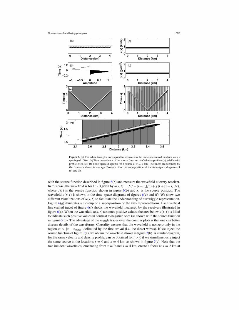
Figure 6. (a) The white triangles correspond to receivers in the one-dimensional medium with aspacing of 100 m. (b) Time dependence of the source function. (c) Velocity profile c(x). (d) Densityprofile "(x). (e), (f) Time–space diagrams for a source at x = 2 km. The traces are recorded bythe receivers shown in (a). (g) Close-up of of the superposition of the time–space diagrams of(e) and (f).

with the source function described in figure 6(b) and measure the wavefield at every receiver.In this case, the wavefield is for t > 0 given by u(x, t) = f (t ! |x ! xs|/c)+ f (t +|x ! xs|/c),where f (t) is the source function shown in figure 6(b) and xs is the source position. Thewavefield u(x, t) is shown in the time–space diagrams of figures 6(e) and (f). We show twodifferent visualizations of u(x, t) to facilitate the understanding of our wiggle representation.Figure 6(g) illustrates a closeup of a superposition of the two representations. Each verticalline (called trace) of figure 6(f) shows the wavefield measured by the receivers illustrated infigure 6(a). When the wavefield u(x, t) assumes positive values, the area below u(x, t) is filledto indicate such positive values in contrast to negative ones (as shown with the source functionin figure 6(b)). The advantage of the wiggle traces over the contour plots is that one can betterdiscern details of the waveforms. Causality ensures that the wavefield is nonzero only in theregion ct > |x ! xsource| delimited by the first arrival (i.e. the direct waves). If we inject thesource function of figure 7(a), we obtain the wavefield shown in figure 7(b). A similar diagram,for the same velocity and density profile, can be obtained for t > 0 if we simultaneously injectthe same source at the locations x = 0 and x = 4 km, as shown in figure 7(c). Note that thetwo incident wavefields, emanating from x = 0 and x = 4 km, create a focus at x = 2 km at


0 1 2 3 40

1

2

3Ti

me

(s)

Distance (km)

!1 !0.5 0 0.5 1

!0.2

0

0.2

Tim

e (s

)Amplitude

(a)

(b)

0 1 2 3 4!3

!2

!1

0

1

2

3

Tim

e (s

)

Distance (km)

0 1 2 3 40

1

2

c S(x

) (km

/s)

Distance (km)

0 1 2 3 40

1

2

! S(x

) (g/

cm3 )

Distance (km)

0 1 2 3 40

1

2

3

Tim

e (s

)

Distance (km)

(d)

(e)

(c)

(f)

Figure 7. (a) Time dependence of the source signal. (b) Time–space diagram for a source atx = 2 km. The traces are recorded by the receivers shown in figure 6(a). (c) Time–space diagramwhen two sources are simultaneously present at x = 0 km and x = 4 km. (d) Velocity profilecs(x). (e) Density profile "s(x). (f) Time–space diagram when a source is present at x = 2 kmin a medium described by cs(x) and "s(x). The traces are recorded by the receivers shown infigure 6(a). The arrow indicates the reflected waves.

t = 0 s. The time–space diagram of figure 7(c) is similar to the light cones described in specialrelativity [26].

This particular time–space diagram is easily created because the medium is homogeneous,but in a more complicated medium this is not trivial. We now consider another one-dimensionalmedium with velocity cs(x) and density "s(x) described in figures 7(d) and (e), respectively.In this case, the medium is not homogeneous; in fact, velocity and density are discontinuous.The incident wavefield emanates from x = 2 km, propagates towards the discontinuity in themodel, interacts with it and generates transmitted and reflected scattered waves. The computedwavefield u(x, t) is presented in the time–space diagram of figure 7(f) and the generation ofthe transmitted and reflected scattered waves is clearly visible at x = 3 km, correspondingto the step in the velocity and density profiles (figures 7(d) and (e)). The heterogeneity hastwo effects. First, there are now reflected waves within the ‘light cone’, as indicated by thearrow in figure 7(f). Second, the arrival time of the waves is crooked because of the changesin velocity.


!1 0 1 2 30

1

2

3

Tim

e (s

)

Distance (km)

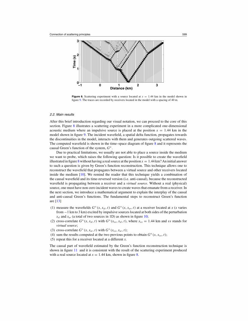
Figure 8. Scattering experiment with a source located at x = 1.44 km in the model shown infigure 9. The traces are recorded by receivers located in the model with a spacing of 40 m.

2.2. Main results

After this brief introduction regarding our visual notation, we can proceed to the core of thissection. Figure 8 illustrates a scattering experiment in a more complicated one-dimensionalacoustic medium where an impulsive source is placed at the position x = 1.44 km in themodel shown in figure 9. The incident wavefield, a spatial delta function, propagates towardsthe discontinuities in the model, interacts with them and generates outgoing scattered waves.The computed wavefield is shown in the time–space diagram of figure 8 and it represents thecausal Green’s function of the system, G+.

Due to practical limitations, we usually are not able to place a source inside the mediumwe want to probe, which raises the following question: Is it possible to create the wavefieldillustrated in figure 8 without having a real source at the position x = 1.44 km? An initial answerto such a question is given by Green’s function reconstruction. This technique allows one toreconstruct the wavefield that propagates between a virtual source and other receivers locatedinside the medium [10]. We remind the reader that this technique yields a combination ofthe causal wavefield and its time-reversed version (i.e. anti-causal), because the reconstructedwavefield is propagating between a receiver and a virtual source. Without a real (physical)source, one must have non-zero incident waves to create waves that emanate from a receiver. Inthe next section, we introduce a mathematical argument to explain the interplay of the causaland anti-causal Green’s functions. The fundamental steps to reconstruct Green’s functionare [13]

(1) measure the wavefields G+(x, xsl, t) and G+(x, xsr, t) at a receiver located at x (x variesfrom !1 km to 3 km) excited by impulsive sources located at both sides of the perturbationxsl and xsr (a total of two sources in 1D) as shown in figure 10;

(2) cross-correlate G+(x, xsl, t) with G+(xvs, xsl, t), where xvs = 1.44 km and vs stands forvirtual source;

(3) cross-correlate G+(x, xsr, t) with G+(xvs, xsr, t);(4) sum the results computed at the two previous points to obtain G+(x, xvs, t);(5) repeat this for a receiver located at a different x.

The causal part of wavefield estimated by the Green’s function reconstruction technique isshown in figure 11 and it is consistent with the result of the scattering experiment producedwith a real source located at x = 1.44 km, shown in figure 8.


!1 0 1 2 30

0.5

1

1.5

2

Vel

ocity

(km

/s)

Distance (km)

!1 0 1 2 30

0.5

1

1.5

2

Den

sity

(g/c

m3 )

Distance (km)

Figure 9. Velocity and density profiles of the one-dimensional model. The perturbation in thevelocity is located between x = 0.3–2.5 km and c0 = 1 km s!1. The perturbation in the density islocated between x = 1.0–2.5 km and "0 = 1 g cm!3.

!1 0 1 2 3

0

1

2

Vel

ocity

(km

/s)

Distance (km)

xsl

xsr

xvs

Figure 10. Diagram showing the locations of the real and virtual sources for seismic interferometry.xsl and xsr indicate the two real sources. xvs shows the virtual source location.

We thus have two different ways to reconstruct the same wavefield, but often we are notable to access a certain portion of the medium we want to study and hence we cannot placeany sources or receivers inside it. We next assume that we only have access to scatteringdata R(t) measured on the left side of the perturbation, i.e. the reflected impulse responsemeasured at x = 0 km due to an impulsive source placed at x = 0 km. This further limitationraises another question: Can we reconstruct the same wavefield shown in figure 8 havingknowledge only of the scattering data R(t)? Since there are neither real sources nor receivers


!1 0 1 2 30

1

2

3

Tim

e (s

)

Distance (km)

Figure 11. Causal part of the wavefield estimated by the Green’s function reconstruction techniquewhen the receiver located at x = 1.44 km acts as a virtual source.

Deltafunction Marchenko equation

Solution of the

t

Figure 12. Incident wave that focuses at location x = 1.44 km and time t = 0 s, built using theiterative process discussed by [15].

inside the perturbation, we speculate that the reconstructed wavefield consists of a causal andan anti-causal part, as shown in figure 14.

For this one-dimensional problem, the answer to this question is given in [15, 27]. Theauthor of [15, 27] shows that we need a particular incident wave in order to collapse thewavefield to a spatial delta function at the desired location after it interacts with the medium,and that this incident wave consists of a spatial delta function followed by the solution of theMarchenko equation, as illustrated in figure 12.

The Marchenko integral equation [6, 28] is a fundamental relation of one-dimensionalinverse scattering theory. It is an integral equation that relates the reflected scattering amplitudeR(t) to the incident wavefield u(t, t f ) which will create a focus in the interior of the medium andultimately gives the perturbation of the medium. The one-dimensional form of this equation is

0 = R(t + t f ) + u(t, t f ) +$ t f

!$R(t + t %)u(t %, t f ) dt %, (1)

where t f is a parameter that controls the focusing location. We solve the Marchenko equation,using the iterative process described in detail in [27], and construct the particular incidentwave that focuses at location x = 1.44 km, as shown in figure 8. After seven steps of theiterative process, we inject the incident wave in the model from the left at x = !1 km andcompute the time–space diagram shown in the top panel of figure 13: it shows the evolution intime of the wavefield when the incident wave is the particular wave computed with the iterative


!1 0 1 2 3!3

!2

!1

0

1

2

3

Tim

e (s

)

!1 0 1 2 30123

Am

plitu

de

Distance (km)

Figure 13. Top: after seven steps of the iterative process described in [27], we inject at x =!1 km the particular incident wave in the model and compute the time–space diagram. Bottom:cross-section of the wavefield at t = 0 s.

method. The bottom panel of figure 13 shows a cross-section of the wavefield at the focusingtime t = 0 s: the wavefield vanishes everywhere except at location x = 1.44 km; hence,the wavefield focuses at this location. Note that the time derivative of the wavefield (i.e. thevelocity) is not focused at x = 1.44 km; hence, the energy is also not focused at this location.We can thus create a focus at a location inside the perturbation without having a source or areceiver at such a location and without any knowledge of the medium properties; we only haveaccess to the reflected impulse response measured on the left side of the perturbation. Withan appropriate choice of sources and receivers, this experiment can be performed in practice(e.g. in a laboratory).

Figure 13 however does not resemble the wavefield shown in figures 8 and 11. But ifwe denote the wavefield in figure 13 as w(x, t) and its time-reversed version as w(x,!t), weobtain the wavefield shown in figure 14 by adding w(x, t) and w(x,!t). With this process,we effectively go from one-sided to two-sided illumination because in figure 14, waves areincident on the scatterer from both sides for t < 0 s. Reference [29] shows similar diagrams andexplains how to combine such diagrams using causality and symmetry properties. The uppercone in figure 14 corresponds to the causal Green’s function and the lower cone representsthe anti-causal Green’s function; the relationship between the two Green’s functions is a keyelement in the next section, where we introduce the homogeneous Green’s function Gh. Note


!1 0 1 2 3!3

!2

!1

0

1

2

3

Tim

e (s

)

Distance (km)

Figure 14. Wavefield that focuses at x = 1.44 km at t = 0 s without a source or a receiver at thislocation. This wavefield consists of a causal (t > 0) and an anti-causal (t < 0) part.

Figure 15. An incident plane wave created by an array of sources is injected in the subsurface.This plane wave is distorted due to the variations in the velocity inside the overburden (i.e. theportion of the subsurface that lies above the scatterer). When the wavefield arrives in the regionthat includes the scatterer, we do not know its shape.

that the wavefield in figure 14, with a focus in the interior of the medium, is based on reflecteddata recorded at the left side of the heterogeneity only. We did not use a source or receiverin the medium, and did not know the medium. All necessary information is encoded in thereflected waves. Note that a small amount of energy is present outside the two cones. This isdue to numerical inaccuracies in our solution of the Marchenko equation.

The extension of the iterative process in two dimensions still needs to be investigated;but we conclude this section with a conjecture illustrated in figure 15. An incident planewave created by an array of sources is injected in the subsurface where it is distorted due tothe variations of the velocity inside the overburden (i.e. the portion of the subsurface that liesabove the scatterer). Since we do not know the characteristics of the wavefield when it interacts


Figure 16. Focusing of the wavefield ‘at depth’. A special incident wave, after interacting with theoverburden, collapses to a point in the subsurface creating a buried source.

xrxA xB x

cs!1 +1

xl

c0

Figure 17. Geometry of the problem for the scattering of acoustic waves in a one-dimensionalmedium with constant density. xA, xB, xl and xr are the coordinates of the receivers (representedby the triangles) and the left and right bounds of our domain, respectively. The perturbation cs issuperposed on a constant velocity profile c0.

with the region of the subsurface that includes the scatterer, it is difficult to reconstruct theproperties of the scatterer without knowing the medium. Hence, following the insights gainedwith the one-dimensional problem, we would like to create a special incident wave that,after interacting with the overburden, collapses to a point in the subsurface creating a buriedsource, as illustrated in figure 16. In this case, assuming that the medium around the scattereris homogeneous, we would know the shape of the wavefield that probes the scatterer andpartially removes the effect of the overburden, which would facilitate accurate imaging of thescatterer.

3. Review of scattering theory

We review the theory for the scattering of acoustic waves in a one-dimensional medium (alsocalled line) with a constant density (in contrast with the previous section where we alsoconsidered variable density), where the scatterer is represented by a perturbation of a constantvelocity profile. Here, we introduce the wave equation and Green’s functions that are used inthe following section of the paper. Figure 17 shows the geometry of the scattering problem.The perturbation cs(x) is superposed on a constant velocity profile c0. The following theoryis developed in the frequency domain because it simplifies the derivations (e.g. convolutionbecomes a multiplication and derivatives become multiplications by !i#). We also showthe time domain version of some of the following equations because they are more intuitiveand allow us to understand the important role played by time reversal. The Fourier transformconvention is defined by f (t) =

!f (#) exp(!i#t) d# and f (#) = (2$ )!1

!f (t) exp(i#t) dt.

Throughout this work, when we deal with a one-dimensional problem, the direction ofpropagation n assumes only two values, 1 and !1, which correspond to waves propagating tothe right and to the left (figure 17), respectively.


The equation that governs the motion of the waves in an unperturbed medium with constantvelocity c0 is the constant-density acoustic homogeneous wave equation

L0(x,#)u0(n, x,#) = 0, (2)

where u0 is the displacement wavefield propagating in the n direction and the differentialoperator is

L0(x,#) #%

d2

dx2+ #2

c20

&. (3)

The solution of equation (2) is u0(n, x,#) = exp(inx#/c0) and its time-domain version isu0(n, x, t) = !(t ! nx/c0), which is a delta function that propagates with velocity c0 in thedirection n representing a physical solution to the wave equation. The unperturbed Green’sfunction satisfies the equation

L0(x,#)G±0 (x, x%,#) = !!(x ! x%), (4)

and, in the acoustic one-dimensional case, its frequency-domain expression is [30]

G±0 (x, x%,#) # ± i

2ke±ik|x!x%|, (5)

where k # #/c0. The + and ! superscripts of Green’s function represent the causal and anti-causal Green’s function with outgoing or ingoing boundary conditions [31], respectively. Inthe time domain, causality implies that

G±0 (x, x%, t) = 0 ± t < |x ! x%|/c0. (6)

Physically, the time-domain Green’s function G+0 (x, x%, t) represents the displacement at a

point x at time t due to a point source of unit amplitude applied at x% at time t = 0, whileG!

0 (x, x%, t) gives the displacement at x that is annihilated by a point source at x% at t = 0.Next we consider the interaction of the wavefield u0 with the perturbation cs(x) (see

figure 17). This interaction produces a scattered wavefield u±sc; hence, the total wavefield can

be represented as u± = u0 + u±sc. The + and ! superscripts in the total wavefield indicate an

initial and a final condition of the wavefield in the time domain, respectively:

u±(n, x, t) & u0(n, x, t) t & '$. (7)

Physically, condition (7) with a plus sign means that the wavefield u+, at early times,corresponds to the initial wavefield u0 propagating forward in time in the n direction. Thecausal and anti-causal wavefields u+ and u! are related by time reversal; in fact, each one isthe time-reversed version of the other u!(t) = u+(!t). In the frequency domain, time reversalcorresponds to complex conjugation: u!(#) = u+"(#). Their time reversal relationship isbetter understood by comparing figures 18(a) and (b), which are valid for the velocity modelof figure 9. Figure 18(b) is obtained by reversing the time axis of figure 18(a). We producedboth figures using the same velocity model we used in section 2 of this paper (figure 9). Infigure 18(a), the initial wavefield is a narrow Gaussian impulse injected at !1.5 km whereasin figure 18(b), the initial wavefield corresponds to the wavefield at t = 6 s in figure 18(a) andit coalesces to an outgoing Gaussian pulse.

The total wavefield u± satisfies the wave equation

L(x,#)u±(n, x,#) = 0, (8)

where the differential operator is

L(x,#) #%

d2

dx2+ #2

c(x)2

&. (9)


!1 !0.5 0 0.5 1 1.5 2 2.50

2

4

6

Tim

e (s

)

Distance (km)

!1 !0.5 0 0.5 1 1.5 2 2.50

2

4

6

Tim

e (s

)

Distance (km)

(a)

(b)

Figure 18. (a) The causal wavefield u+ originated by a narrow Gaussian impulse injected at!1.5 km in the velocity model of figure 9. (b) The anticausal wavefield u!. Note that each panelis the time-reversed version of the other.

The velocity varies with position, c(x) = c0 + cs(x), as illustrated in figure 17. Using theoperator L, we define the perturbed Green’s function as the function that satisfies the equation

L(x,#)G±(x, x%,#) = !!(x ! x%), (10)

with the same boundary conditions as equation (5). Green’s function G± takes into account allthe interactions with the perturbation and hence it corresponds to the full wavefield propagatingbetween the points x% and x, due to an impulsive source at x%.

4. Mathematical tour

In this part of the paper, we lead the reader through a mathematical tour and show that thedifferent scattering principles have a common starting point, i.e. the following fundamentalequation that reveals the connections between them:

G+(xA, xB) ! G!(xA, xB)

='

x%=xl ,xr

m%

G!(x%, xA)ddx

G+(x, xB)|x=x% ! G+(x%, xB)ddx

G!(x, xA)|x=x%

&(11)

with

m =(!1 if x% = xl

+1 if x% = xr,(12)


where xA, xB, xl and xr (see figure 17) are the coordinates of the receivers located at xA

and xB and the left and right bounds of our domain, respectively. Equation (11) (derived inappendix A) shows a relation between the causal and anti-causal Green’s function and we referto this expression, throughout the paper, as the representation theorem for the homogeneousGreen’s function Gh # G+ ! G! [31], which satisfies the wave equation (10) when its sourceterm is set equal to zero. G+ and G! both satisfy the same wave equation (10) because thedifferential operator L is invariant to time reversal (LG+ = !! and LG! = !!); hence, theirdifference is source free: L(G+ ! G!) = 0. The fact that G+ ! G! satisfies a homogeneousequation suggests that a combination of the causal and anti-causal Green’s functions is neededto focus the wavefield at a location where there is no real source. This fact has been illustratedin the previous section when we reconstructed the same wavefield using the Green’s functionreconstruction technique and the inverse scattering theory (see figures 11 and 14); in bothcases, we obtained a combination of the two Green’s functions.

For the remainder of this paper, to be consistent with [32–34], we use the superscripts +

and ! to indicate the causal and anti-causal behaviour of wavefields and Green’s functions,and, for brevity, we omit the dependence on the angular frequency #.

4.1. Newton–Marchenko equation and generalized optical theorem

In this section, we show that equation (11) is the starting point to derive a Newton–Marchenkoequation and a generalized optical theorem. In other words, we demonstrate how lines 1 and3 of table 1 are linked to Gh. The Newton–Marchenko equation differs from the Marchenkoequation because it requires both reflected and transmitted waves as data [35]. In contrastto the Marchenko equation (1), the Newton–Marchenko equation can be extended to twoand three dimensions. The Marchenko and the Newton–Marchenko equations deal with theone-sided and two-sided problem, respectively. Following the work in [32–34], we manipulateequation (11) and show how to derive the equations that rule these two principles. Beforestarting with our derivation, we introduce some useful equations:

u±(n, x) = u0(n, x) + u±sc(n, x)

= u0(n, x) +$

dx%G±0 (x, x%)L%(x%)u±(n, x%), (13)

u±(n, x) = u0(n, x) +$

dx%G±(x, x%)L%(x%)u0(n, x%), (14)

G±(n, x, x%) = G±0 (n, x, x%) +

$dx%%G±(x, x%%)L%(x%%)G±

0 (n, x%%, x%), (15)

f (n, n%) = !$

dx% e!nikx%L%(x%)u+(n%, x%), (16)

where L%(x) # L(x) ! L0(x) describes the influence of the scatterer (perturbation).Equations (13), (14) and (15) are three different Lippmann–Schwinger equations [2]; theyare a reformulation of the scattering problem using linear integral equations with a Green’sfunction kernel. In particular, equation (13) shows that the total field is the summation of theincident wave u0(n, x) and the scattered wave u±

sc(n, x). The integral approach is also wellsuited for the study of inverse problems [8]. Equation (16) is the scattering amplitude [2] foran incident wave travelling in the n direction and that is scattered in the n% direction. We insertequation (15) into (11), simplify considering the fact that xr > xA, x%%, xB and xl < xA, x%%, xB,


and using expression (14)

G+(xA, xB) ! G!(xB, xA) =)

i2k

* )! i

2k

*[iku!(+1, xA)u+(!1, xB)

+ iku+(!1, xB)u!(+1, xA) + iku!(!1, xA)u+(+1, xB)

+ iku+(+1, xB)u!(!1, xA)]. (17)

In a more compact form, this can be written as

G+(xA, xB) ! G!(xB, xA) =)

i2k

* '

n=!1,1

u!(n, xA)u+(!n, xB). (18)

Equation (18) is the starting point to derive a Newton–Marchenko equation; we show the fullderivation in appendix B and write the final result:

u+(+1, xA) ! u!(+1, xA) = ! i2k

'

n=!1,1

u!(n, xA) f (n, xB), xB > xA, x%% (19)

and

u+(!1, xA) ! u!(!1, xA) = ! i2k

'

n=!1,1

u!(n, xA) f (n,!xB), xB < xA, x%%. (20)

The system of coupled equations (19) and (20) is our representation of the one-dimensionalNewton–Marchenko equation [35]. Recognizing that u! = u", equations (19) and (20)correspond to line 1 of table 1.

Next, following a similar derivation that led to equations (19) and (20), we insert expression

u±(n, x) = u0(n, x) +$

dx%G±0 (x, x%)L%(x%)u±(n, x%) (21)

into equation (19), we use the relation u!(n, x) = u+"(!n, x) and equation (16), and wefinally obtain a generalized optical theorem:

f (!n, n) + f "(!n, n) = !'

n%=!1,1

f (!n, n%) f "(n, n%), (22)

where f (n, n%) represents the scattering amplitude [2] and n% assumes the value !1 or +1 (seeline 3 of table 1). The obtained results are exact because in this one-dimensional frameworkwe do not use any far-field approximations.

4.2. Green’s function reconstruction and the optical theorem

Starting from the three-dimensional version of equation (11), reference [36] showed theconnection between the generalized optical theorem and Green’s function reconstruction.Following their three-dimensional formulation, we illustrate the same result for the one-dimensional problem and show the connection between lines 2 and 3 of table 1. In this partof the paper, we show the results and leave the mathematical derivation to appendix C. Theexpression for the one-dimensional Green’s function reconstruction is

i2k

[G+(xA, xB) ! G!(xA, xB)] ='

x%=xl ,xr

G+(xA, x%)G!(xB, x%); (23)

where Green’s function excited by a point source at xB recorded at xA can be separated into anincident and a scattered part and is given by

G±(xA, xB) = ' i2k

e±ik|xB!xA|

+ ,- .direct

' i2k

e±ik|xB| f (n, n%) eik|xA|

+ ,- .scattered

. (24)


xrxA xB xxl 0

0

cs

cs

(a)

(b)

c0

c0

xA xB

c0tA c0tB

Figure 19. Configurations of the system used to show the connection between Green’s functionreconstruction and the optical theorem. In both cases, the receivers xA and xB are located outsidethe scatterer cs, which is located at x = 0.

Unlike the three-dimensional case, we obtain two different results depending on theconfiguration of the system. In the first case (figure 19(a)), the ordinary optical theoremis derived:

f (n, n) + f "(n, n) = !'

n%=!1,1

| f (n, n%)|2; (25)

in the second case (figure 19(b)), we obtain a generalized optical theorem

f (!n, n) + f "(!n, n) = !'

n%=!1,1

f (!n, n%) f "(n, n%), (26)

where n assumes the value !1 or +1.The above expressions of the optical theorem in one dimension agree with the work of the

authors of [37] and differ from their three-dimensional counterpart because they contain the realpart of the scattering amplitude instead of the imaginary part: 2Re f (n, n) # f (n, n)+ f "(n, n),where Re indicates the real part. We note that the ordinary form of the optical theorem (25) alsofollows from its generalized form (26) (the former is a special case of the latter). Furthermore,equation (26) is equivalent to the expression for the optical theorem derived in the previoussection, equation (22). This is not surprising because both equations (26) and (22) have beenderived from the same fundamental equation (11).

5. Conclusions

In section 2, we described the connection between different scattering principles, showingthat there are three distinct ways to reconstruct the same wavefield. A physical source, theGreen’s function reconstruction technique, and inverse scattering theory allow one to createthe same wavestate (see figure 8) originated by an impulsive source placed at a certain locationxs (x = 1.44 km in our examples). Green’s function reconstruction show us how to build anestimate of the wavefield without knowing the medium properties, if we have a receiver atthe same location xs of the real source and sources surrounding the scattering region. Inversescattering goes beyond this and allows us to focus the wavefield inside the medium (at locationxs) without knowing its properties, using only data recorded at one side of the medium. Weshowed that the interaction between causal and anti-causal wavefields is a key element tofocus the wavefield where there is no real source; in fact, Gh = G+ ! G!, which satisfies


the homogeneous wave equation (10), is a superposition of the causal and anti-causal Green’sfunctions.

We speculate that many of the insights gained in our one-dimensional framework are stillvalid in higher dimensions. An extension of this work in two or three dimensions would giveus the theoretical tools for many useful practical applications. For example, if we knew howto create the three-dimensional version of the incident wavefield shown in figure 12, we couldfocus the wavefield to a point in the subsurface to simulate a source at depth and to recorddata at the surface (figure 16); these kind of data are of extreme importance for full waveforminversion techniques [38] and imaging of complex structures (e.g. under salt bodies in seismicexploration [39]). Furthermore, we could possibly concentrate the energy of the wavefieldinside a hydrocarbon reservoir to fracture the rocks and improve the production of oil andgas [40].

In the second part of this paper, the mathematical tour, we demonstrated that therepresentation theorem for the homogeneous Green’s function Gh, equation (11), constitutes atheoretical framework for various scattering principles. We showed that all the principles andtheir equations (see table 1) rely on Gh as a starting point for their derivation. As mentionedabove, the fundamental role played by the combination of the causal and anti-causal Green’sfunctions has been evident throughout the mathematical tour: it is this combination that allowsone to focus the wavefield to a location where neither a real source nor a receiver can beplaced.

Acknowledgments

The authors would like to thank the members of the Center for Wave Phenomena and ananonymous reviewer for their constructive comments. This work was supported by the sponsorsof the Consortium Project on Seismic Inverse Methods for Complex Structures at the Centerfor Wave Phenomena.

Appendix A. Derivation of equation (11)

Here, we derive equation (11), i.e. the representation theorem for the homogeneous Green’sfunction. We start with the equations

d2

dx2G+(x, xB) + #2

c(x)2G+(x, xB) = !!(x ! xB) (A.1)

andd2

dx2G!(x, xA) + #2

c(x)2G!(x, xA) = !!(x ! xA), (A.2)

where xA, xB and x indicate a position between xl and xr in figure 17. Next, we multiplyequation (A.1) by G!(x, xA), and equation (A.2) by G+(x, xB); then, we subtract the tworesults and integrate between xl and xr, yieldingG+(xA, xB) ! G!(xB, xA)

=$ xr

xl

dx%

G!(x, xA)d2

dx2G+(x, xB) ! G+(x, xB)

d2

dx2G!(x, xA)

&. (A.3)

The right-hand side of the last equation is an exact derivative:$ xr

xl

dx%

G!(x, xA)d2

dx2G+(x, xB) ! G+(x, xB)

d2

dx2G!(x, xA)

&

#$ xr

xl

dxddx

%G!(x, xA)

ddx

G+(x, xB) ! G+(x, xB)ddx

G!(x, xA)

&; (A.4)


hence, we obtain the expression for Gh:

G+(xA, xB) ! G!(xA, xB)

='

x%=xl ,xr

m%

G!(x%, xA)ddx

G+(x, xB)|x=x% ! G+(x%, xB)ddx

G!(x, xA)|x=x%

&(A.5)

with

m =(!1 if x% = xl

+1 if x% = xr,(A.6)

where we have used the source–receiver reciprocity relation G±(xA, xB) = G±(xB, xA) for theacoustic Green’s function [41].

Appendix B. Derivation of the Newton–Marchenko equation

Inserting expression (15) into the left-hand side of equation (18), using the relation u+ =u0 + u+

sc on the right-hand side of (18), and then inserting (13) into the right-hand side, we get

e+ik|xA!xB| +$

dx%%G+(xA, x%%)L%(x%%) e+ik|x%%!xB| + e!ik|xA!xB| +$

dx%%G!(xA, x%%)L%(x%%) e!ik|x%%!xB|

= u!(+n, xA) e!ikxB + u+(+n, xA) e+ikxB

+ i2k

u!(+n, xA)

$dx%% e+ik|xB!x%%|L%(x%%)u+(!n, x%%)

+ i2k

u!(!n, xA)

$dx%% e+ik|xB!x%%|L%(x%%)u+(+n, x%%). (B.1)

In this one-dimensional problem, we need to consider two different cases: (1) xB > xA, x%% and(2) xB < xA, x%%. Without loss of generality, we choose xB > xA, x%%, and hence obtain

e+ikxB

%e!ikxA +

$dx%%G+(xA, x%%)L%(x%%) e!ikx%%

&+ e!ikxB

%eikxA +

$dx%%G!(xA, x%%)L%(x%%) e+ikx%%

&

= u!(+1, xA) e!ikxB + u!(!1, xA) e+ikxB ! i2k

u!(+1, xA) e+ikxB

$!dx%% e!ikx%%

L%(x%%)

( u+(!1, x%%)! i2k

u!(!1, xA) e+ikxB

$!dx%% e!ikx%%

L%(x%%)u+(+1, x%%). (B.2)

The terms inside the brackets on the left-hand side correspond to u+(!1, xA) and u!(+1, xA),respectively, whereas the integrals on the right-hand side correspond to f (+1,!1) andf (+1,+1), respectively. We rewrite equation (B.2) using (13), (14) and the relationf (+n,+n%) = f (!n%,!n) to give

u+(+1, xA) ! u!(+1, xA) = ! i2k

'

n=!1,1

u!(n, xA) f (n, xB). (B.3)

For the second case xB < xA, x%%, the solution is

u+(!1, xA) ! u!(!1, xA) = ! i2k

'

n=!1,1

u!(n, xA) f (n,!xB). (B.4)


Appendix C. Green’s function reconstruction and the optical theorem

In this appendix, we derive the mathematics that shows the connection between the Green’sfunction reconstruction equation and the optical theorem in one dimension. The expressionfor Green’s function reconstruction is

i2k

[G+(xA, xB) ! G!(xA, xB)] ='

x%=xl ,xr

G+(xA, x%)G!(xB, x%), (C.1)

and Green’s function excited by a point source at xs recorded at xr is given by

G+(xr, xs) = ! i2k

eik|xs!xr |

+ ,- .T d

! i2k

eik|xs| f (n, n%) eik|xr |

+ ,- .T s

, (C.2)

where f (n, n%) represents the scattering amplitude [2], and n% and n represent the directions ofthe incident wave and the scattered wave, respectively. In the expression above, T d representsthe wave travelling directly from the source to the receiver, and T s corresponds to thescattered wave that reaches the receiver after interacting with the scatterer. Considering thefirst configuration (figure 19(a)), inserting equation (C.2) into the right-hand side of equation(C.1), we get'

x%=xl ,xr

G+(xA, x%)G!(xB, x%) = ! i2k

%! i

2keik(xB!xA ) ! i

2ke!ik(xB+xA ) f (!1, 1)

&

+ ,- .T 1

! i2k

%! i

2ke!ik(xB!xA ) ! i

2keik(xB+xA ) f "(!1, 1)

&

+ ,- .T 2

!)

i2k

*

)i

2k

*eik(xB ! xA )[ f (!1,!1) + f "(!1,!1) + | f (!1,!1)|2 + | f (!1, 1)|2]

+ ,- .T 3

.

(C.3)The terms T 1 and T 2 correspond to G+(xA, xB) and !G!(xA, xB), respectively, while theterm T 3 represents the unphysical wave previously discussed in the mathematical tour; hence,equation (C.3) simplifies to'

x%=xl ,xr

G+(xA, x%)G!(xB, x%) = i2k

[G(xA, xB) ! G!(xA, xB)]

!)

i2k

*2

eik(xB ! xA)[ f (!1,!1)+ f "(!1,!1)+ | f (!1,!1)|2 + | f (!1, 1)|2].

(C.4)For the right-hand side of equation (C.4) to be equal to the left-hand side of equation (C.1),the expression between the square brackets in term T 3 should vanish:

f (!1,!1) + f "(!1,!1) = !| f (!1,!1)|2 + | f (!1, 1)|2. (C.5)Equation (C.5) is the expression for the one-dimensional optical theorem [37]. The secondconfiguration (figure 19(b)) gives'

x%=xl ,xr

G+(xA, x%)G!(xB, x%) = i2k

[G+(xA, xB) ! G!(xA, xB)] !)

i2k

*2

eik(xB+xA )

( [ f (!1, 1) + f "(1,!1) + f (!1,!1) f "(1,!1) + f (!1, 1) f "(1, 1)]+ ,- .T 4

.

(C.6)


In this case, term T 4 corresponds to the generalized optical theorem in onedimension [37].

The connection between Green’s function reconstruction and the generalized opticaltheorem has not only a mathematical proof but also a physical meaning. The cross-correlationof scattered waves in equation (C.3) produces a spurious arrival [36], i.e. an unphysical wavethat is not predicted by the theory. In the first configuration shown in figure 19(a), such spuriousarrival has the same arrival time as the direct wave, tB + tA, but its amplitude is not correct (seeterm T 3 in equation (C.3)). In the second case (figure 19(b)), tA and tB correspond to the timethat a wave takes to travel from the origin x = 0 to xA and xB, respectively. Here, the spuriousarrival corresponds to a wave that arrives at time tB ! tA when no physical wave arrives; in fact,it would arrive before the direct arrival at time tB + tA. But since the ordinary and generalizedoptical theorem hold, the spurious arrival cancels in both cases.

References

[1] Aki K and Richards P G 2002 Quantitative Seismology 2nd edn (Sausalito: University Science Books)[2] Rodberg L S and Thaler R M 1967 Introduction to the Quantum Theory of Scattering (New York: Academic)[3] Born M and Wolf E 1999 Principles of Optics (Cambridge: Cambridge University Press)[4] Shull P J 2002 Nondestructive Evaluation: Theory, Techniques, and Applications (Boca Raton, FL: CRC Press)[5] Epstein C L 2003 Mathematics of Medical Imaging (Upper Saddle River, NJ: Prentice-Hall)[6] Chadan K and Sabatier P C 1989 Inverse Problems in Quantum Scattering Theory 2nd edn (Berlin: Springer)[7] Gladwell G M L 1993 Inverse Problems in Scattering (Alphen aan den Rijn: Kluwer)[8] Colton D and Kress R 1998 Inverse Acoustic and Electromagnetic Scattering Theory (Berlin: Springer)[9] Dorren H J S, Muyzert E J and Snieder R 1994 Inverse Problems 10 865–80

[10] Wapenaar K, Fokkema J and Snieder R 2005 J. Acoust. Soc. Am. 118 2783–6[11] Larose E, Margerin L, Derode A, van Tiggelen B, Campillo M, Shapiro N, Paul A, Stehly L and Tanter M 2006

Geophysics 71 SI11–SI21[12] Bakulin A and Calvert R 2006 Geophysics 71 SI139–SI150[13] Curtis A, Gerstoft P, Sato H, Snieder R and Wapenaar K 2006 Leading Edge 25 1082–92[14] Schuster G T 2009 Seismic Interferometry (Cambridge: Cambridge University Press)[15] Rose J H 2001 Phys. Rev. A 65 012707[16] Rose J H 2002 Time Reversal, Focusing and Exact Inverse Scattering (Imaging of Complex Media with Acoustic

and Seismic Waves) ed M Fink, W A Kuperman, J P Montagner and A Tourin (Berlin: Springer)[17] Claerbout J F 1985 Imaging the Earth’s Interior (Oxford: Blackwell)[18] Sava P and Hill S J 2009 Leading Edge 28 170–83[19] Bleistein N, Cohen J and Stockwell J 2001 Mathematics of Multidimensional Seismic Imaging, Migration, and

Inversion (Berlin: Springer)[20] Biondi B 2006 3D Seismic Imaging (Tulsa, OK: Society of Exploration Geophysicists)[21] Newton R G 1976 Am. J. Phys. 44 639–42[22] Heisenberg W 1943 Z. Phys. 120 673–02[23] Marston P 2001 J. Acoust. Soc. Am. 109 1291[24] Carney P, Schotland J and Wolf E 2004 Phys. Rev. E 70 036611[25] Fokkema J T and van den Berg P M 1993 Seismic Applications of Acoustic Reciprocity (Amsterdam: Elsevier)[26] Ohanian H C and Ruffini R 1994 Gravitation and Spacetime 2nd edn (New York: Norton)[27] Rose J H 2002 Inverse Problems 18 1923–34[28] Lamb G L 1980 Elements of Soliton Theory (New York: Wiley)[29] Burridge R 1980 Wave Motion 2 305–23[30] Snieder R 2004 A Guided Tour of Mathematical Methods for the Physical Sciences 2nd edn (Cambridge:

Cambridge University Press)[31] Oristaglio M 1989 Inverse Problems 5 1097–105[32] Budreck D E and Rose J H 1990 Inverse Problems 6 331–48[33] Budreck D E and Rose J H 1991 SIAM J. Appl. Math. 51 1568–84[34] Budreck D E and Rose J H 1992 J. Math. Phys. 33 2903–15[35] Newton R G 1980 J. Math. Phys. 21 493–505[36] Snieder R, van Wijk K, Haney M and Calvert R 2008 Phys. Rev. E 78 036606[37] Hovakimian L 2005 Phys. Rev. A 72 064701[38] Brenders A J and Pratt R G 2007 Geophys. J. Int. 168 133–51[39] Sava P and Biondi B 2004 Geophys. Prospect. 52 607–23[40] Beresnev I A and Johnson P A 1994 Geophysics 59 1000–17[41] Wapenaar K and Fokkema J 2006 Geophysics 71 SI33–SI46

Documents

Connection of scattering principles: a visual and ...inside.mines.edu/~rsnieder/Broggini_EJP12.pdfConnection of scattering principles: a visual and mathematical tour ... Connection