Embed Size (px)
Citation preview
Connectivity and giant component in randomirrigation graphs
Gabor Lugosi
ICREA and Pompeu Fabra University, Barcleona
joint work withNicolas Broutin (INRIA)Luc Devroye (McGill)
irrigation graphs
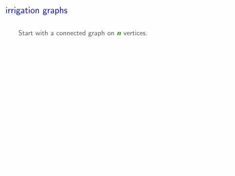
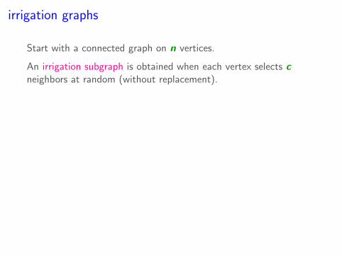
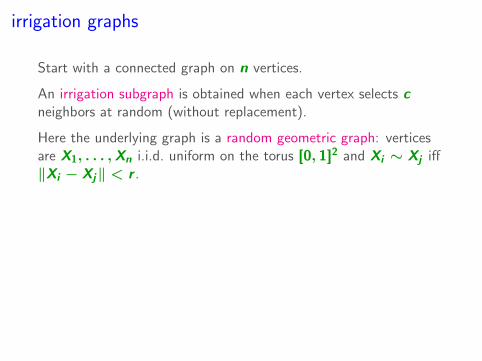
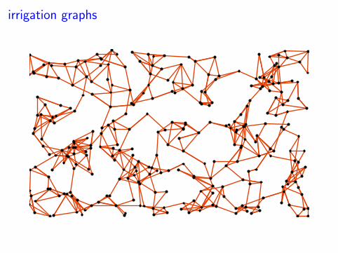
Start with a connected graph on n vertices.
An irrigation subgraph is obtained when each vertex selects cneighbors at random (without replacement).
Here the underlying graph is a random geometric graph: verticesare X1, . . . ,Xn i.i.d. uniform on the torus [0, 1]2 and Xi ∼ Xj iff‖Xi − Xj‖ < r .
Also called bluetooth graphs.They are locally sparsified random geometric graphs.
Introduced by Ferraguto, Mambrini, Panconesi, and Petrioli (2004).
Fenner and Frieze (1982) considered Kn as the underlying graph.
Question: How large does c need to be for G(n, r , c) to beconnected?
irrigation graphs
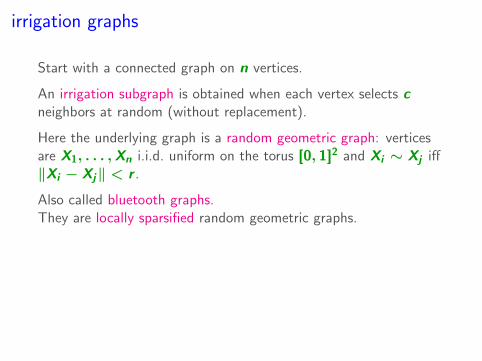
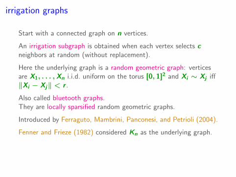
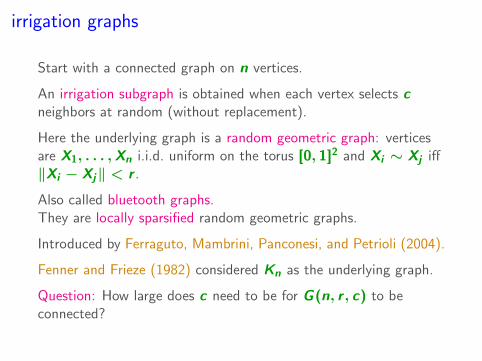
Start with a connected graph on n vertices.
An irrigation subgraph is obtained when each vertex selects cneighbors at random (without replacement).
Here the underlying graph is a random geometric graph: verticesare X1, . . . ,Xn i.i.d. uniform on the torus [0, 1]2 and Xi ∼ Xj iff‖Xi − Xj‖ < r .
Also called bluetooth graphs.They are locally sparsified random geometric graphs.
Introduced by Ferraguto, Mambrini, Panconesi, and Petrioli (2004).
Fenner and Frieze (1982) considered Kn as the underlying graph.
Question: How large does c need to be for G(n, r , c) to beconnected?

irrigation graphs
G(n, r) needs to be connected.
Connectivity threshold is r∗ ∼√
log n/(πn).
We only consider r ≥ γ√
log n/n for a sufficiently large γ.
irrigation graphs
G(n, r) needs to be connected.
Connectivity threshold is r∗ ∼√
log n/(πn).
We only consider r ≥ γ√
log n/n for a sufficiently large γ.
irrigation graphs
G(n, r) needs to be connected.
Connectivity threshold is r∗ ∼√
log n/(πn).
We only consider r ≥ γ√
log n/n for a sufficiently large γ.
irrigation graphs
irrigation graphs
irrigation graphs
previous results
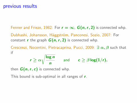
Fenner and Frieze, 1982: For r =∞, G(n, r , 2) is connected whp.
Dubhashi, Johansson, Haggstrom, Panconesi, Sozio, 2007: Forconstant r the graph G(n, r , 2) is connected whp.
Crescenzi, Nocentini, Pietracaprina, Pucci, 2009: ∃ α, β such thatif
r ≥ α√
log nn
and c ≥ β log(1/r),
then G(n, r , c) is connected whp.
This bound is sub-optimal in all ranges of r .

previous results
Fenner and Frieze, 1982: For r =∞, G(n, r , 2) is connected whp.
Dubhashi, Johansson, Haggstrom, Panconesi, Sozio, 2007: Forconstant r the graph G(n, r , 2) is connected whp.
Crescenzi, Nocentini, Pietracaprina, Pucci, 2009: ∃ α, β such thatif
r ≥ α√
log nn
and c ≥ β log(1/r),
then G(n, r , c) is connected whp.
This bound is sub-optimal in all ranges of r .

previous results
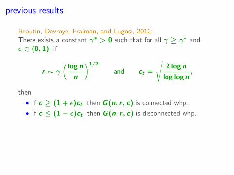
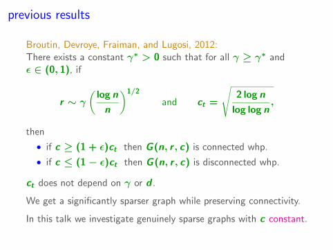
Broutin, Devroye, Fraiman, and Lugosi, 2012:There exists a constant γ∗ > 0 such that for all γ ≥ γ∗ andε ∈ (0, 1), if
r ∼ γ(
log nn
)1/2
and ct =
√2 log n
log log n,
then
• if c ≥ (1 + ε)ct then G(n, r , c) is connected whp.
• if c ≤ (1− ε)ct then G(n, r , c) is disconnected whp.
ct does not depend on γ or d .
We get a significantly sparser graph while preserving connectivity.
In this talk we investigate genuinely sparse graphs with c constant.
previous results
Broutin, Devroye, Fraiman, and Lugosi, 2012:There exists a constant γ∗ > 0 such that for all γ ≥ γ∗ andε ∈ (0, 1), if
r ∼ γ(
log nn
)1/2
and ct =
√2 log n
log log n,
then
• if c ≥ (1 + ε)ct then G(n, r , c) is connected whp.
• if c ≤ (1− ε)ct then G(n, r , c) is disconnected whp.
ct does not depend on γ or d .
We get a significantly sparser graph while preserving connectivity.
In this talk we investigate genuinely sparse graphs with c constant.
sparse connectivity by enlarging r
The lower bound follows from a more general result:
Let ε ∈ (0, 1) and λ ∈ [1,∞] be such that r > γ∗(
log nn
)1/2
log nr2
log log n→ λ and c ≤ (1− ε)
√(λ
λ− 1/2
)log n
log nr2.
Then G(n, r , c) is disconnected whp.

sparse connectivity by enlarging r
The lower bound follows from a more general result:
Let ε ∈ (0, 1) and λ ∈ [1,∞] be such that r > γ∗(
log nn
)1/2
log nr2
log log n→ λ and c ≤ (1− ε)
√(λ
λ− 1/2
)log n
log nr2.
Then G(n, r , c) is disconnected whp.
sparse connectivity by enlarging r
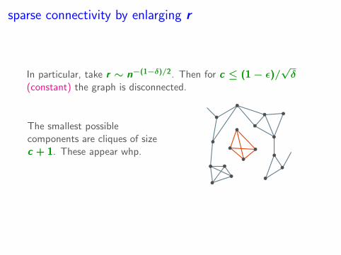
In particular, take r ∼ n−(1−δ)/2. Then for c ≤ (1− ε)/√δ
(constant) the graph is disconnected.
The smallest possiblecomponents are cliques of sizec + 1. These appear whp.
sparse connectivity by enlarging r
In particular, take r ∼ n−(1−δ)/2. Then for c ≤ (1− ε)/√δ
(constant) the graph is disconnected.
The smallest possiblecomponents are cliques of sizec + 1. These appear whp.

connectivity for constant c
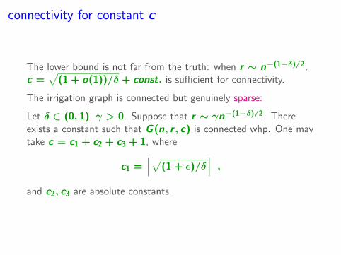
The lower bound is not far from the truth: when r ∼ n−(1−δ)/2,c =
√(1 + o(1))/δ + const. is sufficient for connectivity.
The irrigation graph is connected but genuinely sparse:
Let δ ∈ (0, 1), γ > 0. Suppose that r ∼ γn−(1−δ)/2. Thereexists a constant such that G(n, r , c) is connected whp. One maytake c = c1 + c2 + c3 + 1, where
c1 =⌈√
(1 + ε)/δ⌉,
and c2, c3 are absolute constants.
connectivity for constant c
The lower bound is not far from the truth: when r ∼ n−(1−δ)/2,c =
√(1 + o(1))/δ + const. is sufficient for connectivity.
The irrigation graph is connected but genuinely sparse:
Let δ ∈ (0, 1), γ > 0. Suppose that r ∼ γn−(1−δ)/2. Thereexists a constant such that G(n, r , c) is connected whp. One maytake c = c1 + c2 + c3 + 1, where
c1 =⌈√
(1 + ε)/δ⌉,
and c2, c3 are absolute constants.

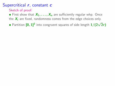
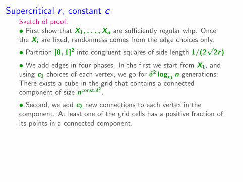
Supercritical r , constant cSketch of proof:• First show that X1, . . . ,Xn are sufficiently regular whp. Oncethe Xi are fixed, randomness comes from the edge choices only.
• Partition [0, 1]2 into congruent squares of side length 1/(2√
2r)
• We add edges in four phases. In the first we start from X1, andusing c1 choices of each vertex, we go for δ2 logc1
n generations.There exists a cube in the grid that contains a connectedcomponent of size nconst.δ2
.
• Second, we add c2 new connections to each vertex in thecomponent. At least one of the grid cells has a positive fraction ofits points in a connected component.
• Third, using c3 new connections of each vertex, we obtain aconnected component that contains a constant fraction of thepoints in every cell of the grid, whp.
• Finally, add just one more connection per vertex so that theentire graph becomes connected.
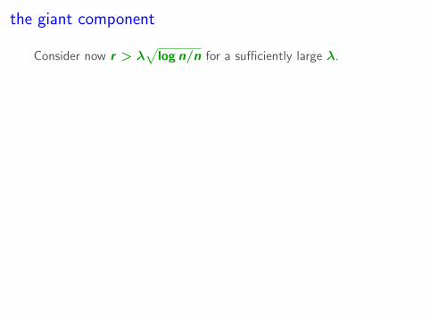
the giant component
Consider now r > λ√
log n/n for a sufficiently large λ.
It is not difficult to see that for c = 1 the size of the largestcomponent is at most poly-logarithmic.
It is o(n) even for much larger values of r .
To study the phase transition, we generalize the model. Eachvertex xi draws a bounded independent integer-valued randomvariable ξi ≥ 1 and selects ξi neighbors at random (withoutreplacement).
Main result: for any ε > 0, if Eξi ≥ 1 + ε, then the size of thelargest component is n(1− o(1)) whp.
Explosive percolation: the phase transition is discontinuous. Wehave even more: the proportion of vertices in the giant componentjumps from 0 to 1. We have super-explosive percolation.
explosive percolation
the giant component: formal statement
For every δ ∈ (0, 1) there exists a γ > 0 such that for everyε > 0, if r ≥ γ
√log n/n and Eξ > 1 + ε, then the largest
component has size at least n(1− δ) whp.
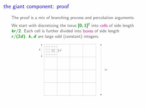
the giant component: proof
The proof is a mix of branching process and percolation arguments.
We start with discretizing the torus [0, 1]2 into cells of side lengthkr/2. Each cell is further divided into boxes of side lengthr/(2d). k, d are large odd (constant) integers.
m
k d
uniformity lemma
During the entire proof we fix the vertex set X .
We need that they are sufficiently regularly placed.
One can prove that if γ > 12d 2/δ2 then whp every box B isδ-good:
(1− δ)nr2
4d 2≤ |X ∩ B| ≤
(1 + δ)nr2
4d 2.
This gives us a condition on r :
r ≥ γ√
log nn
uniformity lemma
During the entire proof we fix the vertex set X .
We need that they are sufficiently regularly placed.
One can prove that if γ > 12d 2/δ2 then whp every box B isδ-good:
(1− δ)nr2
4d 2≤ |X ∩ B| ≤
(1 + δ)nr2
4d 2.
This gives us a condition on r :
r ≥ γ√
log nn
uniformity lemma
During the entire proof we fix the vertex set X .
We need that they are sufficiently regularly placed.
One can prove that if γ > 12d 2/δ2 then whp every box B isδ-good:
(1− δ)nr2
4d 2≤ |X ∩ B| ≤
(1 + δ)nr2
4d 2.
This gives us a condition on r :
r ≥ γ√
log nn

the web
In the first phase of the proof we prove the existence of a web:
Let ε > 0. There exist δ, k, d such that if all cells are δ-good,then with probability at least 1− ε, G(n, r , c) has a connected
component such that 1− ε fraction of all boxes contain E[ξ]k2/2
vertices of the component.
This is the heart of the proof. We set up an exploration processand then couple it with a percolation model.
node events
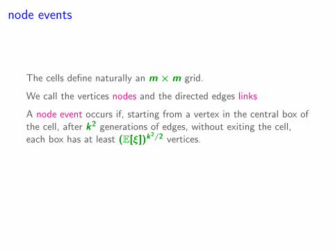
The cells define naturally an m ×m grid.
We call the vertices nodes and the directed edges links
A node event occurs if, starting from a vertex in the central box ofthe cell, after k2 generations of edges, without exiting the cell,each box has at least (E[ξ])k2/2 vertices.
By coupling the growth process to a branching random walk, weshow that a node event occurs with probability close to 1.
node events
The cells define naturally an m ×m grid.
We call the vertices nodes and the directed edges links
A node event occurs if, starting from a vertex in the central box ofthe cell, after k2 generations of edges, without exiting the cell,each box has at least (E[ξ])k2/2 vertices.
By coupling the growth process to a branching random walk, weshow that a node event occurs with probability close to 1.
link events
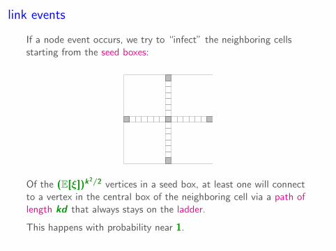
If a node event occurs, we try to “infect” the neighboring cellsstarting from the seed boxes:
Of the (E[ξ])k2/2 vertices in a seed box, at least one will connectto a vertex in the central box of the neighboring cell via a path oflength kd that always stays on the ladder.
This happens with probability near 1.
link events
If a node event occurs, we try to “infect” the neighboring cellsstarting from the seed boxes:
Of the (E[ξ])k2/2 vertices in a seed box, at least one will connectto a vertex in the central box of the neighboring cell via a path oflength kd that always stays on the ladder.
This happens with probability near 1.
exploration process
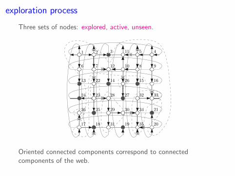
Three sets of nodes: explored, active, unseen.
21 3 45
6 7 9810
11
12
13 14 15 16
17 18 19 20
21
22
2324
25
26
2728
29 30
31
32 33
34
35
36
Oriented connected components correspond to connectedcomponents of the web.

mixed site/bond percolation
After the exploration process, all node events and some link eventsare defined. (All independent!)
We assign independent Bernoulli variables to all undefined orientedlinks.
We declare a bond open if both oriented links are open.
This defines a dense mixed site/bond percolation process on thegrid. Any open component is an oriented connected component.
Using results of Deuschel and Pisztora (1996) for high-density sitepercolation, we conclude that there is an open componentcontaining 1− ε fraction of the nodes. This gives us the web.
connecting to the web
We constructed the web by revealing the edge choices of only aconstant number ((E[ξ])k2/2) of vertices per cell.
Once the web is built, we connect almost all unseen vertices.
Take such a vertex. Build a new web starting from this point. Thetwo webs will “see” each other in Θ(1/r2) boxes and connect upwith probability 1/(nr2) at each point.
The probability that any vertex is connected to the web is1− o(1).