Connector Algebras, Petri Nets, and BIP?

Roberto Bruni1, Hernan Melgratti2, and Ugo Montanari1

1 Dipartimento di Informatica, Universita di Pisa, Italy2 Departamento de Computacion, Universidad de Buenos Aires - Conicet, Argentina

Abstract. In the area of component-based software architectures, theterm connector has been coined to denote an entity (e.g. the communica-tion network, middleware or infrastructure) that regulate the interactionof independent components. Hence, a rigorous mathematical foundationfor connectors is crucial for the study of coordinated systems. In recentyears, many different mathematical frameworks have been proposed tospecify, design, analyse, compare, prototype and implement connectorsrigorously. In this paper, we overview the main features of three notableframeworks and discuss their similarities, differences, mutual embeddingand possible enhancements. First, we show that Sobocinski’s nets withboundaries are as expressive as Sifakis et al.’s BI(P), the BIP componentframework without priorities. Second, we provide a basic algebra of con-nectors for BI(P) by exploiting Montanari et al.’s tile model and a recentcorrespondence result with nets with boundaries. Finally, we exploit thetile model as a unifying framework to compare BI(P) with other modelsof connectors and to propose suitable enhancements of BI(P).

1 Introduction

Recent years have witnessed an increasing interest about a rigorous modellingof (different classes of) connectors. The term connector, as used here, has beencoined within the area of component-based software architectures, to name enti-ties that can regulate the interaction of a collection of components [27]. This hasled to the development of different mathematical frameworks that are used tospecify, design, analyse, compare, prototype and implement suitable connectors.As such connectors have been often designed by research groups with differentbackground and having different aims in mind (e.g. efficient verification of em-bedded system, generality and extensibility, implementability over a distributedarchitecture), many existing proposals are built over specific features that on theone hand complicate a comparison in terms of expressiveness and on the otherhand make it difficult to enhance one model with additional features comingfrom another model. Similarly, one were to enhance all models with the same

? Research supported by European FET-IST-257414 Integrated Project ASCENS,ANPCyT Project BID-PICT-2008-00319, and UBACyT 20020090300122. The travelexpenses of Ugo Montanari for participating to PSI’11 have been supported by For-mal Methods Europe.

2

new feature, then different solutions would be required. As an example, no uni-form agreement about how to define dynamically reconfigurable connectors hasbeen set up yet.

In this paper, we overview our recent advancements towards a unifying theoryof connectors by focussing on the comparison of three notable connector frame-works, namely the BIP component framework [6], Petri nets with boundaries [30]and the algebras of connectors [11, 2] based on the tile model [20, 9]. The mainresult establishes that BIP without priorities, written BI(P) in the following, isequally expressive to nets with boundaries. Thanks to the correspondence re-sults in [30, 12], we can define an algebra of connectors as expressive as BI(P),where a few basic connectors can be composed in series and parallel to generateany BI(P) system. The algebra is a suitable instance of the tile model, which wepropose as unifying framework for the study of connectors. In fact, the generalityof the tile model as a general semantic framework has been already witnessedin [26, 14, 18, 16, 24, 21, 13].

Connectors basics. Component-based design relies on the separation of con-cerns between coordination and computation. Component-based systems arebuilt from sequential computational entities, the components, that should beloosely coupled w.r.t. the concurrent execution environments where they willbe deployed. The component interfaces comprise the number, kind and pecu-liarities of communication ports. The communication media that make possibleto interact are called connectors. They can be regarded as (suitably decorated)links between the ports of the components. Graphically, ports are representedas nodes and connectors as hyperarcs whose tentacles are attached to the portsthey control. Several connectors can also be combined together by merging someof the ports their tentacles are attached to. Semantically, each connector canimpose suitable constraints on the communications between the components itlinks together. For example, a connector may impose handshaking between asender component and a receiver component (CCS synchronization). A differentkind of connector may require global consensus on the next action to perform(Hoare synchronization) or it may trigger the broadcasting of a message sentfrom one component to all the other linked components. The evolution of a net-work of components and connectors (just network for brevity) can be seen as ifplayed in rounds: At each round, the components try to interact through theirports and the connectors allow/disallow some of the interactions selectively. Aconnector is called stateless when the interaction constraints it imposes over itsports stays the same at each round; it is called stateful otherwise. To addresscomposition and modularity of a system, networks are often decorated with in-put and output interfaces: in the simpler cases, they consist of ports throughwhich a network can interact. For example, two networks can be composed bymerging the ports (i.e. nodes) they have in common. Ports that are not in theinterface are typically private to the network and cannot be used to attach ad-ditional connectors. The distinction between input and output ports indicatesin which direction the data should flow, but feedback is also possible throughshort-circuit connectors.

3

(i)

◦ s //α �� T

◦β��

◦t// ◦

(ii)

◦ //

�� T1

◦ //

�� T2

◦��

◦ // ◦ // ◦(iii)

◦ //

�� T1

◦��

◦ //

�� T2

◦��

◦ // ◦

(iv)

◦ //

��◦��◦ //

��◦��

T2

◦ // ◦◦ //T1 ◦

Fig. 1. Examples of tiles and their composition

The BIP component framework. BIP [6] is a component framework for con-structing systems by superposing three layers of modelling: 1) Behaviour, thelower level, representing the sequential computation of individual components;2) Interaction, the middle layer, defining the handshaking mechanisms betweenthese components; and 3) Priority, the top level, assigning a partial order ofprivileges to the admissible synchronisations. The lower layer consists of a setof atomic components with ports, modelled as automata whose arcs are labelledby sets of ports. The sets of ports of any two different components are disjoint,i.e., each port is uniquely assigned to a component. The second layer consists ofconnectors that specify the allowed interactions between components. Roughly,connectors define suitable relations between ports. The third layer exploits pri-orities to enforce scheduling policies over allowed interactions, typically with theaim of reducing the size of the state space. One supported feature of BIP is theso-called correctness by construction, which allows the specification of architec-ture transformations preserving certain properties of the underlying behaviour.For instance it is possible to provide (sufficient) conditions for compositional-ity and composability which guarantee deadlock-freedom. The BIP componentframework has been implemented in a language and a tool-set. In absence ofpriorities, the interaction layer of BIP admits the algebraic presentation givenin [7].

The tile model The Tile Model [20, 9] offers a flexible and adequate semanticsetting for concurrent systems [26, 18, 15] and also for defining the operationaland abstract semantics of suitable classes of connectors.

A tile T : sα−→βt is a rewrite rule stating that the initial configuration s can

evolve to the final configuration t via α, producing the effect β; but the step isallowed only if the ‘arguments’ of s can contribute by producing α, which acts asthe trigger of the rewrite. The name ‘tile’ is due to the graphical representationof such rules (see Fig. 1(i)). Triggers and effects are called observations and tilevertices are called interfaces.

Tiles can be composed horizontally, in parallel, or vertically to generate largersteps. Horizontal composition T1;T2 coordinates the evolution of the initial con-figuration of T1 with that of T2, yielding the ‘synchronization’ of the two rewrites(see Fig. 1(ii)). Horizontal composition is possible only if the initial configura-tions of T1 and T2 interact cooperatively: the effect of T1 must provide the

4

trigger for T2. Vertical composition is sequential composition of computations(see Fig. 1(iii)). The parallel composition builds concurrent steps (see Fig. 1(iv)).

Roughly, the semantics of component-based systems can be expressed via tileswhen: i) components and connectors are equipped with sequential compositions; t (defined when the output interface of s matches the input interface of t) andwith a monoidal tensor product s ⊗ t (associative, with unit and distributingover sequential composition); ii) observations have analogous structure α;β andα ⊗ β. Technically, we require that configurations and observations form twomonoidal categories [25] with the same underlying set of objects.

Tiles express the reactive behaviour of connectors in terms of trigger/effectpairs of labels (α, β). In this context, the usual notion of bisimilarity over thederived Labelled Transition System is called tile bisimilarity. Tile bisimilarity isa congruence (w.r.t. composition in series and parallel) when a simple tile formatis met by basic tiles [20].

The wire calculus The wire calculus [29] shares strong similarities with the tilemodel, in the sense that it has sequential and parallel compositions and exploitstrigger-effect pairs labels as observations. However it is presented as a processalgebra instead of via monoidal categories and it exploits a different kind ofvertical composition. Each process comes with an input/output arity typing,e.g., we write ` P : (n,m) for P with n input ports and m output ports. Theusual action prefixes a.P of process algebras are extended in the wire calculusby the simultaneous input of a trigger a and output of an effect b, written a

b .P ,where a (resp. b) is a string of actions, one for each input port (resp. outputport) of the process.

In [30] a dialect of the wire calculus has been used to give an exact char-acterisation of a special class of (stateful) connectors that can be alternativelyexpressed in terms of so-called Petri nets with boundaries. Technically speaking,the contribution in [30] can be summarized as follows. Nets with boundaries arefirst introduced, taking inspiration from the open nets of [5]. Nets with bound-aries can be composed in series and in parallel and come equipped with a labelledtransition system that fixes their operational and bisimilarity semantics. Then, asuitable instance of the wire calculus from [29] is presented, called Petri calculus,that roughly models circuit diagrams with one-place buffers and interfaces. Thefirst result enlightens a tight semantics correspondence: it is shown that a Petricalculus process can be defined for each net such that the translation preservesand reflects operational semantics (and thus also bisimilarity). The second re-sult provides the converse translation, from Petri calculus to nets, which requiressome technical ingenuity. The work in [30] has been recently improved in [12]by showing that if the tile model is used in place of the wire calculus then thetranslation from Petri calculus to nets becomes simpler and that the main re-sults of [30] can be extended to P/T Petri nets with boundaries, where arcs areweighted and places can contain more than one token.

Structure of the paper. In § 2 we recall the main definition and notation for BIPand nets with boundaries. In § 3 we prove that BI(P) and nets with boundaries

5

are equally expressive. In § 4 we exploit the results in § 3 and in [30, 12] to definea suitable algebra of BI(P) systems and compare it with the work in [8]. Wediscuss related work in § 5. Some concluding remarks and open issues for futurework are in § 6.

2 Background

2.1 The BIP component framework

This section reports on the formal definition of BIP as presented in [8]. Since wedisregard priorities, we call BI(P) the framework presented here.

Definition 1 (Interaction). Given a set of ports P , an interaction over P isa non-empty subset a ⊆ P .

We write an interaction {p1, p2, . . . , pn} as p1p2 . . . pn and a ↓Pifor the pro-

jection of an interaction a ⊆ P over the set of ports Pi ⊆ P , i.e., a ↓Pi= a ∩ Pi.

Projection extends to sets of interactions in the following way γ ↓P= {a ↓P | a ∈γ ∧ a ↓P 6= ∅}.

Definition 2 (Component). A component B = (Q,P,→) is a transition sys-tem where Q is a set of states, P is a set of ports, and →⊆ Q × 2P ×Q is theset of labelled transitions.

As usual, we write qa−→ q′ to denote the transition (q, a, q′) ∈→. We let

q ∵ a ∴ q′ be the name of the transition qa−→ q′. Given a transition t = q ∵ a ∴ q′,

we let ◦t, t◦ and λ(t) denote respectively its source q, its target q′ and its label

a. An interaction a is enabled in q, denoted qa−→, iff there exists q′ s.t. q

a−→ q′.

By abusing notation, we will also write q∅−→ q for any q.

Definition 3 (BI(P) system). A BI(P) system B = γ(B1, . . . , Bn) is thecomposition of a finite set {Bi}ni=1 of transitions systems Bi = (Qi, Pi,→i)such that their sets of ports are pairwise disjoint, i.e., Pi ∩ Pj = ∅ for i 6= jparameterized by a set γ ⊂ 2P of interactions over the set of ports P =

⊎ni=1 Pi.

We call P the underlying set of ports of B, written ι(B).

The semantics of a BIP system γ(B1, . . . , Bn) is given by the transition sys-tem (Q,P,→γ), with Q = ΠiQi, P =

⊎ni=1 Pi and →γ⊆ Q× 2P ×Q is the least

set of transitions satisfying the following inference rule

a ∈ γ ∀i ∈ 1..n : qia↓Pi−−−→ q′i

(q1, . . . , qn)a−→γ (q′1, . . . , q

′n)

Example 1. Figure 2 shows a simple BIP system consisting of three transitionssystems B1, B2, and B3 and the synchronization γ = {ab, cd, d}.

6

γ = {ab, cd, d}B1 B2 B3

q1 aff q2

b ((q3 bff

chh q4 dff

ι(B1) = {a} ι(B2) = {b, c} ι(B3) = {d}

Fig. 2. A simple BIP system B = γ(B1, B2, B3)

2.2 Nets with boundaries

Petri nets [28] consist of places (i.e. resources types), which are repositories oftokens (i.e., resource instances), and transitions that remove and produce tokens.

Definition 4 (Net). A net N is a 4-tuple N = (SN , TN ,◦−N ,−◦N ) where SN

is the (nonempty) set of places, a, a′, . . ., TN is the set of transitions, t, t′, . . .(with SN ∩ TN = ∅), and the functions ◦−N ,−◦N : TN → 2SN assign finite setsof places, called respectively source and target, to each transition.

Transitions t, u are independent when ◦t ∩ ◦u = t◦ ∩ u◦ = ∅. This no-tion of independence allows so-called contact situations. Moreover, it also allowsconsume/produce loops, i.e., a place p can be both in ◦t and t◦. A set U of tran-sitions is mutually independent when, for all t, u ∈ U , if t 6= u then t and u areindependent. Given a set of transitions U let ◦U = ∪u∈U ◦u and U◦ = ∪u∈Uu◦.

Definition 5 (Semantics). Let N = (P, T, ◦−,−◦) be a net, X,Y ⊆ P andt ∈ T . Write:

(N,X)→{t} (N,Y )def= ◦t ⊆ X ∧ t◦ ⊆ Y ∧X\◦t = Y \t◦

For U ⊆ T a set of mutually independent transitions, write:

(N,X)→U (N,Y )def= ◦U ⊆ X ∧ U◦ ⊆ Y ∧X\◦U = Y \U◦

Note that, for any X ⊆ P , (N,X) →∅ (N,X). States of this transitionsystem will be referred to as markings of N .

The remaining of this section recalls the composable nets proposed in [30].

In the following we let k, l, m, n range over finite ordinals: ndef= {0, 1, . . . , n−1}.

Definition 6 (Nets with boundaries). Let m,n ∈ N. A net with boundariesN : m → n is a tuple N = (S, T, ◦−,−◦, •−,−•) where (S, T, ◦−,−◦) is a netand functions •− : T → 2m and −• : T → 2n assign transitions to the left andright boundaries of N , respectively.

7

•

��

α //��

•

•

��

WW

•

==

β //??

•(a) P .

•

��

α //��

•

��•

WW

•

==

β //??

•(b) Q.

•

��

// γ //•

δ //•(c) R.

Fig. 3. Three nets with boundaries

The representation of the left and right boundaries as ordinals is just a nota-tional convenience. In particular, we remark that the left and the right bound-aries of a net are always disjoint.

The notion of independence of transitions extends to nets with boundariesin the obvious way: t, u ∈ T are said to be independent when

◦t ∩ ◦u = ∅ ∧ t◦ ∩ u◦ = ∅ ∧ •t ∩ •u = ∅ ∧ t• ∩ u• = ∅

The obvious notion of net homomorphism between nets with equal bound-aries just requires that source, target, left and right boundaries are preserved,and a homomorphism is an isomorphism iff its two components (places and tran-sitions) are bijections. We write N ∼= M when there is an isomorphism from Nto M .

Example 2. Figure 3 shows two different nets with boundaries. Places are circlesand a marking is represented by the presence or absence of tokens; rectangles aretransitions and arcs stand for pre and postset relations. The left interface (rightinterface) is depicted by points situated on the left (respectively, on the right).Figure 3(a) shows the net P : 2→ 2 containing two places, two transitions andone token. Net Q is similar to P , but has a different initial marking. Differentlyfrom P and Q, R has just one node in its left interface.

Nets with boundaries can be composed in parallel and in series. Given N :m → n and M : k → l, their tensor product is the net N ⊗M : m + k → n + lwhose sets of places and transitions are the disjoint union of the correspondingsets in N and M , whose maps ◦−,−◦, •−,−• are defined according to the mapsin N and M and whose initial marking is m0N ⊕m0M . Intuitively, the tensorproduct corresponds to put the nets N and M side-by-side.

The sequential composition N ;M : m → k of N : m → n and M : n → kis slightly more involved and relies on the following notion of synchronization: apair (U, V ) with U ⊆ TN and V ⊆ TM mutually independent sets of transitionssuch that: (1) U ∪ V 6= ∅ and (2) U• = •V .

The set of synchronisations inherits an ordering from the subset relation, i.e.(U, V ) ⊆ (U ′, V ′) when U ⊆ U ′ and V ⊆ V ′. A synchronisation is said to beminimal when it is minimal with respect to this order. Let

TN ;Mdef= {(U, V )|U ⊆ TN , V ⊆ TM , (U, V ) a minimal synchronisation}

8

αγ //

��

•

αδ //

''

•

•

00

((

•

||

•

..

66 bb

TT

βγ //

77

•

βδ //

GG

•

Fig. 4. Net P ; (R⊕R)

Notice that any transition t in N (respectively t′ in M) not connected tothe shared boundary n defines a minimal synchronisation ({t},∅) (respectively(∅, {t′})) in the above sense. The sequential composition of N and M is writtenN ;M : m → k and defined as (SN ] SM , TN ;M ,

◦−N ;M ,−◦N ;M ,•−N ;M ,−•N ;M ),

where pre- and post-sets of synchronizations are defined as

– ◦(U, V )N ;M = ◦(U)N ] ◦(V )M and (U, V )◦N ;M = (U)◦N ] (V )◦M– •(U, V )N ;M = •(U)N and (U, V )•N ;M = (V )•M .

Intuitively, transitions attached to the left or right boundaries can be seenas transition fragments, that can be completed by attaching other complemen-tary fragments to that boundary. When two transition fragments in N share aboundary node, then they are two mutually exclusive options for completing afragment of M attached to the same boundary node. Thus, the idea is to combinethe transitions of N with that of M when they share a common boundary, as iftheir firings were synchronized. As in general several combinations are possible,only minimal synchronizations are selected, because the other can be recoveredas concurrent firings.

Sometimes we find convenient to write N = (S, T, ◦−,−◦, •−,−•, X) withX ⊆ S for the net (S, T, ◦−,−◦, •−,−•) with initial marking X and extend thesequential and parallel composition to nets with initial marking by taking theunion of the initial markings.

Example 3. Consider the nets P and R in Figure 3. Then, the net P ; (R ⊗ R)obtained as the composition of P and R is shown in Figure 4.

For any k ∈ N, there is a bijection p q : 2k → {0, 1}k with

pUqidef={

1 if i ∈ U0 otherwise

9

Definition 7 (Semantics). Let N : n→ n be a net and X,Y ⊆ PN . Write:

(N,X)α−→β

(N,Y )def= ∃ mutually independent U ⊆ TN s.t

(N,X)→U (N,Y ), α = p•Uq, and β = pU•q

3 Encoding BIP into nets

This section studies the correspondence between BI(P) systems and nets. Westart by showing that any BI(P) system can be mapped into a bisimilar net (§3.1).Then, we introduce a notion of composition of BI(P) systems (§3.2) and then, byexploiting compositionality of nets with boundaries, we provide a compositionalencoding of BI(P) systems into nets with boundaries (§3.3).

3.1 Monolithic Mapping

It is folklore that a BIP system can be seen as 1-safe Petri net with priorities.This section shows a concrete mapping of a BI(P) system into a net.

Definition 8. Let B = γ(B1, . . . , Bn) be a BI(P) system. The correspondingnet is NB = (P, T, ◦−N ,−◦N ) where P = ι(B),

T = {〈q1 ∵ a ↓P1∴ q′1, . . . , qn ∵ a ↓Pn

∴ q′n〉 |a ∈ γ ∧ a = ]i(a ↓Pi) ∧ ∀i ∈ 1..n : (qi ∈ Qi ∧ qi

a↓Pi−−−→ q′i)}

with ◦− : T → 2P and −◦ : T → 2P s.t.

◦〈q1 ∵ a ↓P1∴ q′1, . . . , qn ∵ a ↓Pn

∴ q′n〉 = {qi | a ↓Pi6= ∅}

〈q1 ∵ a ↓P1∴ q′1, . . . , qn ∵ a ↓Pn∴ q

′n〉◦ = {q′i | a ↓Pi 6= ∅}

Given a transition t = 〈q1 ∵ a ↓P1∴ q′1, . . . , qn ∵ a ↓Pn∴ q

′n〉, we let a be the

label of t, i.e., λ(t) = a.Intuitively, the places of the netNB are in one-to-one correspondence with the

states of the components, while the transitions of NB represent the synchronizedexecution of transitions on the components.

Example 4. Consider the BI(P) system B = γ(B1, B2, B3) shown in Figure 2.The net NB corresponding to the BI(P) system is shown in Figure 5. Note thatthe net contains as many transitions as the allowed synchronizations amongcomponents. For instance, the net has two different transitions that match theinteraction ab, any of them describing one possible synchronization betweencomponents B1 and B2. In fact, interaction ab is possible when B1 executes

q1a−→ q1 and B2 does either q2

b−→ q3 or q3b−→ q3.

Theorem 1 (Correspondence). Let B = γ(B1, . . . , Bn) be a BI(P) system.

Then, (q1, . . . , qn)a−→γ (q′1, . . . , q

′n) iff (NB , {q1, . . . , qn})→{t} (NB , {q′1, . . . , q′n})

and λ(t) = a.

Proof. The result straightforwardly follows by construction of the net. �

10

q1 ∵ a ∴ q1, q3 ∵ b ∴ q3

rr ##

q4 ∵ d ∴ q4

��q1

55

##

q2

��

q3

cc

##

q4

HH

��q1 ∵ a ∴ q1, q2 ∵ b ∴ q3

cc 22

q3 ∵ c ∴ q2, q4 ∵ d ∴ q4

ii GG

Fig. 5. Mapping of the BI(P) system Nγ(B1,B2,B3) into a net

3.2 Composite BI(P) Systems

In this section we introduced a notion of composition for BI(P) systems thatallows to take BI(P) systems as components of larger systems. We start byintroducing a notion of coherence between interactions that will be used fordefining allowed compositions of BI(P) systems.

Definition 9 (Coherent interaction extension). Given two sets of interac-tions γ and γ′ we say that γ′ is a coherent extension of γ over the set of portsP , written γ .P γ

′, iff γ′ ↓P⊆ γ.

The idea underlying coherent extension is that the extended set of interac-tions γ′ does not allow more interactions between the ports in P than thosespecified by γ.

Definition 10 (Composite BI(P) system). A composite BI(P) system iseither a BI(P) system C = γ(B1, . . . , Bn) or a composition γ(C1, . . . , Cn) where{Ci = γi(Ci,1, . . . , Ci,ni

)}ni=1 is a family of composite BI(P) systems such thattheir sets of underlying ports are pairwise disjoint, i.e., ι(Ci) ∩ ι(Cj) = ∅ fori 6= j, and γ a set of interactions over ]ni=1ι(Ci) s.t. γi .ι(Ci) γ.

Note that the definition of composite BI(P) systems generalizes the notionof BI(P) systems. In fact, any transition system B = (Q,P,→) can be seen asa BI(P) system 2P (B), i.e., a BI(P) system composed by exactly one transitionsystem whose allowed interactions are all possible combination of ports (i.e., anypossible label in 2P is allowed by the interaction 2P ). It is straightforward toshow that B and 2P (B) have isomorphic transitions systems.

The semantics of composite BI(P) systems is defined analogously to that ofBI(P) systems by viewing each subsystem as a component.

Next result states that any BI(P) system can be seen as a composite BI(P)system of exactly two components. We will use this property when defining thecompositional encoding of BI(P) systems.

Lemma 1. Let B = γ(B1, . . . , Bn) be a BI(P) system. Then, for any i < n, Bis bisimilar to the composite BI(P) system C = γ(γ ↓P1..i (B1, . . . , Bi), γ ↓P\P1..i

(Bi−1, . . . , Bn)) where P = ι(B) and P1..i = ]j≤iι(Bj).

Proof. The proof follows by straightforward coinduction. �

11

q1

ab��q2

(a) Transition System.

q1

��

•a

q1 ∵ ab ∴ q2

��

88

&&q2 •b

(b) Corresponding Net with boundaries.

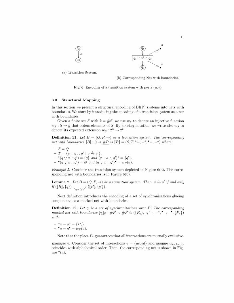
Fig. 6. Encoding of a transition system with ports {a, b}

3.3 Structural Mapping

In this section we present a structural encoding of BI(P) systems into nets withboundaries. We start by introducing the encoding of a transition system as a netwith boundaries.

Given a finite set S with k = #S, we use wS to denote an injective functionwS : S → k that orders elements of S. By abusing notation, we write also wS todenote its expected extension wS : 2S → 2k.

Definition 11. Let B = (Q,P,→) be a transition system. The correspondingnet with boundaries [[B]] : 0→ #P is [[B]] = (S, T, ◦−,−◦, •−,−•) where:

– S = Q– T = {q ∵ a ∴ q′ | q a−→ q′}.– ◦(q ∵ a ∴ q′) = {q} and (q ∵ a ∴ q′)◦ = {q′}.– •(q ∵ a ∴ q′) = ∅ and (q ∵ a ∴ q′)• = wP (a).

Example 5. Consider the transition system depicted in Figure 6(a). The corre-sponding net with boundaries is in Figure 6(b).

Lemma 2. Let B = (Q,P,→) be a transition system. Then, qa−→ q′ if and only

if ([[B]], {q}) −−−−−→pwP (a)q

([[B]], {q′}).

Next definition introduces the encoding of a set of synchronizations glueingcomponents as a marked net with boundaries.

Definition 12. Let γ be a set of synchronizations over P . The correspondingmarked net with boundaries [[γ]]P : #P → #P is ({Pγ}, γ, ◦−,−◦, •−,−•, {Pγ})with

– ◦a = a◦ = {Pγ}.– •a = a• = wP (a).

Note that the place Pγ guarantees that all interactions are mutually exclusive.

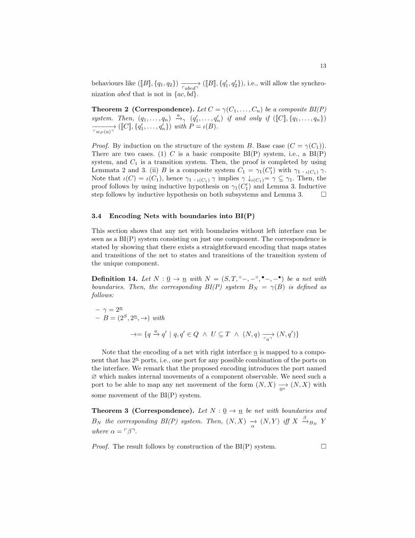
Example 6. Consider the set of interactions γ = {ac, bd} and assume w{a,b,c,d}coincides with alphabetical order. Then, the corresponding net is shown in Fig-ure 7(a).

12

• ''aac %%

��

��

•a

•��

b•

II

��

•b

•

<<

cbd

22

��

XX

•c

•

22

d•d

(a)[[{ac, bd}]]{a,b,c,d}.

q1

��

[[B1]]

• //a

a //

��

[[γ ↓{a,b}]]{a,b}

•

��

a

[[γ]]{a,b,c,d}

•a

q1 ∵ ab ∴ q′1

��

77

''

•

FF

��

ac

22

��

��

q′1 • //b

b //

XX

•

��

b•

II

��

•b

q2

��

• //c

c //

��

•

>>

cbd

22

��

XX

•c

q2 ∵ cd ∴ q′2

��''

77

•

FF

��q′2

[[B2]]

• //d

d //

XX

[[γ ↓{c,d}]]{c,d}

•

>>

d•d

(b) [[γ(B1, B2)]] with γ = {ac, bd}.

Fig. 7. Compositional encoding

Lemma 3. Let γ be a set of interactions over P . Then, [[γ]]PpwP (a)q−−−−−→pwP (a)q

[[γ]]P iff

a ∈ γ.

Proof. It follows from the definition of [[γ]]P . �

Next definition introduces the compositional encoding of BI(P) systems.

Definition 13. Let B = γ(B1, . . . , Bn) be a composite BI(P) system. The cor-responding net with boundaries [[B]] : 0 → #P with P = ι(B) is recursively

defined as 3

[[γ(B1)]] = [[B1]]; [[γ]]P[[γ(B1, . . . , Bn)]] = (γ ↓P1

[[B1]]⊗ [[γ ↓P\P1(B2, . . . , Bn)]]); [[γ]]P

with P1 = ι(B1)

Example 7. Consider the BI(P) system B = {ac, bd}(B1, B2) where B1 has just

one transition q1ab−→ q′1 and B2 has only q2

cd−→ q′2. The encoded net is in Fig-ure 7(b). Note the necessity of considering all transitions in the encoding of{ac, bd} to be mutual exclusive. Otherwise, the encoded form will also allow

3 For technical convenience we define the encoding of γ(B1, . . . , Bn) in terms of aparticular partition of the system: one subsystem containing just one component,i.e. B1, and the other formed by the remaining components B2, . . . , Bn. We remarkthat the results in this paper can be formulated by considering any possible partitionof the system.

13

behaviours like ([[B]], {q1, q2}) −−−−→pabcdq

([[B]], {q′1, q′2}), i.e., will allow the synchro-

nization abcd that is not in {ac, bd}.

Theorem 2 (Correspondence). Let C = γ(C1, . . . , Cn) be a composite BI(P)

system. Then, (q1, . . . , qn)a−→γ (q′1, . . . , q

′n) if and only if ([[C]], {q1, . . . , qn})

−−−−−→pwP (a)q

([[C]], {q′1, . . . , q′n}) with P = ι(B).

Proof. By induction on the structure of the system B. Base case (C = γ(C1)).There are two cases. (1) C is a basic composite BI(P) system, i.e., a BI(P)system, and C1 is a transition system. Then, the proof is completed by usingLemmata 2 and 3. (ii) B is a composite system C1 = γ1(C ′1) with γ1 .ι(C1) γ.Note that ι(C) = ι(C1), hence γ1 .ι(C1) γ implies γ ↓ι(C1)= γ ⊆ γ1. Then, theproof follows by using inductive hypothesis on γ1(C ′1) and Lemma 3. Inductivestep follows by inductive hypothesis on both subsystems and Lemma 3. �

3.4 Encoding Nets with boundaries into BI(P)

This section shows that any net with boundaries without left interface can beseen as a BI(P) system consisting on just one component. The correspondence isstated by showing that there exists a straightforward encoding that maps statesand transitions of the net to states and transitions of the transition system ofthe unique component.

Definition 14. Let N : 0 → n with N = (S, T, ◦−,−◦, •−,−•) be a net withboundaries. Then, the corresponding BI(P) system BN = γ(B) is defined asfollows:

– γ = 2n

– B = (2S , 2n,→) with

→= {q a−→ q′ | q, q′ ∈ Q ∧ U ⊆ T ∧ (N, q) −−→paq

(N, q′)}

Note that the encoding of a net with right interface n is mapped to a compo-nent that has 2n ports, i.e., one port for any possible combination of the ports onthe interface. We remark that the proposed encoding introduces the port named∅ which makes internal movements of a component observable. We need such aport to be able to map any net movement of the form (N,X) −→

0n(N,X) with

some movement of the BI(P) system.

Theorem 3 (Correspondence). Let N : 0 → n be net with boundaries and

BN the corresponding BI(P) system. Then, (N,X) −→α

(N,Y ) iff Xβ−→BN

Y

where α = pβq.

Proof. The result follows by construction of the BI(P) system. �

14

R ::= © | ©· | I | X | ∇ | ∇

| ⊥ | > | ∧ | ∨ | ↓ | ↑ | R⊗R | R;R

Fig. 8. Petri calculus grammar

R : (k, l) R′ : (m,n)

R⊗R′ : (k +m, l + n)

R : (k, n) R′ : (n, l)

R;R′ : (k, l)

Fig. 9. Sort inference rules

© 1−→0©· ©· 0−→

1© ©· 1−→

1©· I

1−→1

I ∇ 1−→11∇

∇11−→1

∇

⊥ 1−→ ⊥ > −→1>

Xxy−→yx

X ∧ 1−→xx∧ ∨ xx−→

1∨

R1α−→σR2 R′

1σ−→βR′

2

R1;R′1α−→βR2;R′

2

R1α−→βR2 R′

1ρ−→σR′

2

R1 ⊗R′1ασ−−→βρ

R2 ⊗R′2

R : (m,n)

R0m−−→0n

R

Fig. 10. Operational semantics for the Petri Calculus

4 The BIP algebra of connectors

Thanks to the result in § 3, we are now ready to provide a finite algebra forgenerating all BI(P) systems. The algebra we propose is the algebra of statelessconnectors from [11], enriched with one-place buffers along [2, 30, 12]. We call itPetri calculus after [30]. Terms of the Petri Calculus are defined by the gram-mar in Fig. 8. It consists of the following constants plus parallel and sequentialcomposition: the empty place ©, the full place ©· , the identity wire I, the twist(also swap, or symmetry) X, the duplicator (also sync) ∇ and its dual

∇

, themutex (also choice) ∧ and its dual ∨, the hiding (also bang) ⊥ and its dual >,the inaction ↓ and its dual ↑.

Any term has a unique associated sort (also called type) (k, l) with k, l ∈ N,that fixes the size k of the left (input) interface and the size l of the right (output)interface of P . The type of constants are as follows:©,©· , and I have type (1, 1),X : (2, 2), ∇ and ∧ have type (1, 2) and their duals

∇

and ∨ have type (2, 1),⊥ and ↓ have type (1, 0) and their duals > and ↑ have type (0, 1). The sortinference rules for composed processes are in Fig. 9.

The operational semantics is defined by the rules in Fig. 10, where x, y ∈{0, 1} and we let x = 1−x. The labels α, β, ρ, σ of transitions are binary strings,

all transitions are sort-preserving, and if Rα−→β

R′ with R,R′ : (n,m), then

|α| = n and |β| = m. Notably, bisimilarity induced by such a transition systemis a congruence.

Example 8. For example, let R1def= (∇⊗∇); (©· ⊗X⊗©); (

∇

⊗

∇

);X and R2def=

(∇⊗∇); (©⊗X⊗©· ); (

∇

⊗

∇

);X. It is immediate to check that both R1 and R2

15

have sort (2, 2), in fact we have: ∇⊗∇ : (2, 4), ©· ⊗X⊗© : (4, 4), ©⊗X⊗©· :

(4, 4),

∇

⊗

∇

: (4, 2), and of course X : (2, 2). The only moves for R1 are R100−→00

R1

and R101−→10

R2 while the only moves for R2 are R200−→00

R2 and R210−→01

R1. It is

immediate to note that R1 and R2 are terms analogous to the nets in Fig. 3 andthat R1 is bisimilar to X;R2;X.

A close correspondence between nets with boundaries and Petri calculusterms is established in [30], by providing mutual encodings with tight semanticscorrespondence. First, it is shown that any net N : m→ n with initial markingX can be associated with a term TN,X : (m,n) that preserves and reflects thesemantics of N . Conversely, for any term T : (m,n) of the Petri calculus thereexists a bisimilar net NT : m→ n. Due to space limitation we omit details hereand refer the interested reader to [30].

Corollary 1. The Petri calculus and BI(P) have the same expressive power.

Proof. We know from [30, 12] that the Petri calculus is as expressive as netswith boundaries, in the sense that given a net with boundaries we can find abisimilar Petri calculus process and vice versa. The results in Section 3 showthe analogous correspondence between nets with boundaries and BI(P) systems.Then, the thesis just follows by transitivity. �

It is interesting to compare the Petri calculus with the algebra of causalinteraction trees from [8], generated by the grammar:

t ::= a | a→ t | t⊕ t

where a is an interaction. As a matter of notation, we can write t→ t′ meaning:

t→ t′ =

{a→ (t1 ⊕ t′) if t = a→ t1(t1 → t′)⊕ (t2 → t′) if t = t1 ⊕ t2

Intuitively, the causality operator → imposes a as a trigger of t in a → t(so that t can take part in a global interaction only if a does so), while the(associative and commutative) parallel composition operator ⊕ compose possiblealternative. Without loss of generality, we shall assume that in t⊕ t′ and t→ t′

the ports in t and t′ are disjoint.

Example 9. Classical examples (taken from [8]) of interaction policies repre-sented by the algebra of causal interaction trees over ports a, b, c and d are:the rendezvous abcd; the broadcast a → (b ⊕ c ⊕ d) corresponding to the set{a, ab, ac, ad, abc, abd, acd, abcd}; the atomic broadcast a → bcd correspondingto the set {a, abcd}; and the causal chain a → b → c → d corresponding to theset {a, ab, abc, abcd}.

The algebra of causal interaction trees has the advantage of distinguishingbroadcast from a set of rendezvous by allowing to render the causal dependency

16

relation between ports in an explicit way. Moreover, it allows to simplify expo-nentially complex models that cannot be a basis for efficient implementation andit induces a semantic equivalence that is also a congruence.

We can provide a direct translation from this algebra to the Petri calculus.To this aim, we fix some usual notation from the literature, that generalizesthe simple connector constants to larger interfaces. Let k > 0, then we defineIk : (k, k), Xk : (1 + k, 1 + k), and ∧k : (k, 2k) as below:

I1 = I Ik+1 = I⊗ IkX1 = X Xk+1 = (X⊗ Ik); (I⊗ Xk)∧1 = ∧ ∧k+1 = (∧ ⊗ ∧k); (I⊗ Xk ⊗ Ik)

Intuitively, Ik is the identity wiring, Xk swap the first port with the otherk − 1 ports, and ∧k : (k, 2k) splits a series of k ports.

Moreover, for α ∈ {0, 1}k a binary string of length k > 0, we let Rα : (k, 1)denote the process inductively defined by:

R0 =↓;> R1 = I Rxα = (Rx ⊗Rα);

∇

Intuitively, the term Rα synchronizes the ports associated to the positions of αthat are set to 1.

We are now ready to encode causal interaction trees to Petri calculus pro-cesses. Let P a set of ports, n = #P and t a causal interaction tree over P . Wedefine the Petri calculus process [[t]]P : (n, 1) by structural induction as below.

[[a]]P = RpwP (a)q

[[t⊕ t′]]P = ∧n; ([[t]]P ⊗ [[t′]]P ); (∧ ⊗ ∧); (I⊗

∇

⊗ I); (∨ ⊗ I);∨[[t→ t′]]P = ∧n; ([[t]]P ⊗ [[t′]]P ); (∧ ⊗ I); (I⊗

∇

);∨

The encodings [[a]]P is straightforward. The encoding [[t ⊕ t′]]P is obtainedby first evaluating t and t′ over the same input interface (see the sub-process∧n; ([[t]]P ⊗ [[t′]]P )), then by requiring that either t and t′ synchronize or that oneof them executes alone. The encoding [[t → t′]]P is analogous, but now either tand t′ synchronize, or t executes alone.

Lemma 4. The process [[t]]P is stateless for any t, i.e., whenever [[t]]Pα−→β

R′

then R′ = [[t]]P .

Proof. The thesis follows simply by noting that [[t]]P is composed out of statelessconnectors, i.e., the encoding does not exploit the constants ©,©· . �

At the semantic level, the correspondence between t and [[t]]P : (n, 1) can bestated as follows.

Proposition 1. Let t be a causal interaction tree, let I(t) denote the set of

interactions allowed by t and let R = [[t]]P . Then, a ∈ I(t) iff RpwP (a)q−−−−−→

1R.

Proof. The proof is by structural induction on t. �

17

5 Related work

In [11], an algebra of stateless connectors was presented that was inspired byprevious work on simpler algebraic structures [10, 31]. It consists of five kinds ofbasic connectors (plus their duals), namely symmetry, synchronization, mutualexclusion, hiding and inaction. The connectors can be composed in series or inparallel. The operational, observational and denotational semantics of connectorsare first formalised separately and then shown to coincide. Moreover, a completenormal-form axiomatisation is available for them. These networks are quite ex-pressive: for instance it is shown [11] that they can model all the (stateless)connectors of the architectural design language CommUnity [19]. The encodingshown in § 4 shows that it is as expressive as the algebra of causal interactiontrees. The algebra of stateless connectors in [11] can be regarded as a peculiarkind of tile model where all basic tiles have identical initial and final connectors,i.e. they are of the form s

a−→bs. In terms of the wire calculus, this means that only

recursive processes of the form recX.ab .X are considered for composing largernetworks of connectors. The comparison in [11] is of particular interest, becauseit reconciles the algebraic and categorical approaches to system modelling, ofwhich the algebra of stateless connectors and CommUnity are suitable represen-tatives. The algebraic approach models systems as terms in a suitable algebra.Operational and abstract semantics are then usually based on inductively de-fined labelled transition systems. The categorical approach models systems asobjects in a category, with morphisms defining relations such as subsystem orrefinement. Complex software architectures can be modelled as diagrams in thecategory, with universal constructions, such as colimit, building an object in thesame category that behaves as the whole system and that is uniquely determinedup to isomorphisms. While in the algebraic approach equivalence classes are usu-ally abstract entities, having a normal form gives a concrete representation thatmatches a nice feature of the categorical approach, namely that the colimit of adiagram is its best concrete representative.

Reo [1] is an exogenous coordination model for software components. Reois based on channel-like connectors that mediate the flow of data and signalsamong components. Notably, a small set of point-to-point primitive connectorsis sufficient to express a large variety of interesting constraints over the behaviourof connected components, including various forms of mutual exclusion, synchro-nization, alternation, and context-dependency. Typical primitive connectors arethe synchronous/asynchronous/lossy channels and the asynchronous one-placebuffer. They are attached to ports called Reo nodes. Components and primi-tive connectors can be composed into larger Reo circuits by disjoint union up-tothe merging of shared Reo nodes. The semantics of Reo has been formalized inseveral ways, exploiting co-algebraic techniques [3], constraint-automata [4], col-oring tables [17], and the tile model [2]. Differently from the stateless connectorsof [11], Reo connectors are stateful (in particular due to the asynchronous one-place buffer connector). Nevertheless, it has been shown in [2] that the 2-coloursemantics of Reo connectors can be recovered into the setting of the basic algebra

18

of connectors and in the tile approach by adding a connector and a tile for theone-state buffer. It is worth mentioning that, in addition, the tile semantics ofReo connectors provides a description for full computations instead of just singlesteps (as considered in the original 2-colour semantics) and makes evident theevolution of the connector state (particularly, whether buffers get full or becomeempty).

The problem of interpreting BIP interaction models (i.e., the second layer ofBIP) in terms of connectors has been addressed for the first time in [7], whereBIP interaction is described as a structured combination of two basic synchro-nization primitives between ports: rendezvous and broadcast. In this approach,connectors are described as sets of possible interactions among involved ports. Inparticular, broadcasts are described by the set of all possible interactions amongparticipating ports and thus the distinction between rendezvous and broadcastbecomes blurred. The main drawback of this approach is that it induces anequivalence that is not a congruence. The paper [8] defines a causal semanticsthat does not reduce broadcast into a set of rendezvous and tracks the causaldependency relation between ports. In particular, the semantics based on causalinteraction trees allows to simplify exponentially complex models that cannotbe a basis for efficient implementation.

The Petri calculus approach [30] takes inspiration from the tile model andfrom the so-called Span(Graph) model [22, 23]. The paper [30] is particularlyinteresting in our opinion because it relates for the first time process calculi andPetri nets via a finite set of basic connectors.

6 Conclusion

One of the main limitations of the state-of-the-art theories of connectors isthe lack of a reference paradigm for describing and analysing the informationflow to be imposed over components for proper coordination. Such a paradigmwould allow designers, analysts and programmers to rely on well-founded andstandard concepts instead of using all kinds of heterogeneous mechanisms, likesemaphores, monitors, message passing primitives, event notification, remotecall, etc. Moreover, the reference paradigm would facilitate the comparison andevaluation of otherwise unrelated architectural approaches as well as the devel-opment of code libraries for distributed connectors. To some extent, the referenceparadigm could thus play the role of a unifying semantic framework for connec-tors.

We conjecture that the algebraic properties of the tile model can help re-lating formal frameworks that are otherwise very different in style and nature(CommUnity, Reo, Petri nets with boundaries, wire calculus). For instance, whilecompositionality needs often ad hoc proofs when other approaches are consid-ered, in the case of the tile model, it can be expressed in terms of the congruenceresult for tile bisimilarity and it can be guaranteed by the format in which basictiles are presented.

19

The most interesting and challenging research avenue for future work is therepresentation of priorities in approaches such as the Petri calculus and the tilemodel.

References

1. F. Arbab. Reo: a channel-based coordination model for component composition.Mathematical Structures in Computer Science, 14(3):329–366, 2004.

2. F. Arbab, R. Bruni, D. Clarke, I. Lanese, and U. Montanari. Tiles for Reo. InA. Corradini and U. Montanari, editors, WADT, volume 5486 of LNCS, pages37–55. Springer, 2009.

3. F. Arbab and J. J. M. M. Rutten. A coinductive calculus of component connectors.In M. Wirsing, D. Pattinson, and R. Hennicker, editors, WADT, volume 2755 ofLNCS, pages 34–55. Springer, 2002.

4. C. Baier, M. Sirjani, F. Arbab, and J. J. M. M. Rutten. Modeling componentconnectors in Reo by constraint automata. Sci. Comput. Program, 61(2):75–113,2006.

5. P. Baldan, A. Corradini, H. Ehrig, and R. Heckel. Compositional semantics for openpetri nets based on deterministic processes. Mathematical Structures in ComputerScience, 15(1):1–35, 2005.

6. A. Basu, M. Bozga, and J. Sifakis. Modeling heterogeneous real-time componentsin BIP. In Fourth IEEE International Conference on Software Engineering andFormal Methods (SEFM 2006), pages 3–12. IEEE Computer Society, 2006.

7. S. Bliudze and J. Sifakis. The algebra of connectors - structuring interaction inBIP. IEEE Trans. Computers, 57(10):1315–1330, 2008.

8. S. Bliudze and J. Sifakis. Causal semantics for the algebra of connectors. FormalMethods in System Design, 36(2):167–194, 2010.

9. R. Bruni. Tile Logic for Synchronized Rewriting of Concurrent Systems. PhD the-sis, Computer Science Department, University of Pisa, 1999. Published as TechnicalReport TD-1/99.

10. R. Bruni, F. Gadducci, and U. Montanari. Normal forms for algebras of connection.Theor. Comput. Sci., 286(2):247–292, 2002.

11. R. Bruni, I. Lanese, and U. Montanari. A basic algebra of stateless connectors.Theor. Comput. Sci., 366(1-2):98–120, 2006.

12. R. Bruni, H. Melgratti, and U. Montanari. A connector algebra for P/T netsinteractions. In J.-P. Katoen and B. Koenig, editors, CONCUR, volume 6901 ofLNCS, pages 312–326. Springer, 2011.

13. R. Bruni, J. Meseguer, and U. Montanari. Symmetric monoidal and cartesiandouble categories as a semantic framework for tile logic. Mathematical Structuresin Computer Science, 12(1):53–90, 2002.

14. R. Bruni and U. Montanari. Cartesian closed double categories, their lambda-notation, and the pi-calculus. In LICS, pages 246–265, 1999.

15. R. Bruni and U. Montanari. Dynamic connectors for concurrency. Theor. Comput.Sci., 281(1-2):131–176, 2002.

16. R. Bruni, U. Montanari, and F. Rossi. An interactive semantics of logic program-ming. TPLP, 1(6):647–690, 2001.

17. D. Clarke, D. Costa, and F. Arbab. Connector colouring I: Synchronisation andcontext dependency. Sci. Comput. Program, 66(3):205–225, 2007.

20

18. G. L. Ferrari and U. Montanari. Tile formats for located and mobile systems. Inf.Comput., 156(1-2):173–235, 2000.

19. J. L. Fiadeiro and T. S. E. Maibaum. Categorical semantics of parallel programdesign. Sci. Comput. Program., 28(2-3):111–138, 1997.

20. F. Gadducci and U. Montanari. The tile model. In G. D. Plotkin, C. Stirling,and M. Tofte, editors, Proof, Language, and Interaction, pages 133–166. The MITPress, 2000.

21. F. Gadducci and U. Montanari. Comparing logics for rewriting: rewriting logic,action calculi and tile logic. Theor. Comput. Sci., 285(2):319–358, 2002.

22. P. Katis, N. Sabadini, and R. F. C. Walters. Representing place/transition netsin Span(Graph). In M. Johnson, editor, AMAST, volume 1349 of LNCS, pages322–336. Springer, 1997.

23. P. Katis, N. Sabadini, and R. F. C. Walters. Span(Graph): A categorial algebra oftransition systems. In M. Johnson, editor, AMAST, volume 1349 of LNCS, pages307–321. Springer, 1997.

24. B. Konig and U. Montanari. Observational equivalence for synchronized graphrewriting with mobility. In N. Kobayashi and B. C. Pierce, editors, TACS, volume2215 of LNCS, pages 145–164. Springer, 2001.

25. S. MacLane. Categories for the Working Mathematician (2nd edition). Springer,1998.

26. U. Montanari and F. Rossi. Graph rewriting, constraint solving and tiles for coor-dinating distributed systems. Applied Categorical Structures, 7(4):333–370, 1999.

27. D. E. Perry and E. L. Wolf. Foundations for the study of software architecture.ACM SIGSOFT Software Engineering Notes, 17:40–52, 1992.

28. C. Petri. Kommunikation mit Automaten. PhD thesis, Institut fur InstrumentelleMathematik, Bonn, 1962.

29. P. Sobocinski. A non-interleaving process calculus for multi-party synchronisation.In F. Bonchi, D. Grohmann, P. Spoletini, and E. Tuosto, editors, ICE, volume 12of EPTCS, pages 87–98, 2009.

30. P. Sobocinski. Representations of petri net interactions. In P. Gastin andF. Laroussinie, editors, CONCUR, volume 6269 of LNCS, pages 554–568. Springer,2010.

31. G. Stefanescu. Reaction and control I. mixing additive and multiplicative networkalgebras. Logic Journal of the IGPL, 6(2):348–369, 1998.