Consequences of Consumer Sales Taxes in Light of Strategic Suppliers

Anil Arya

The Ohio State University

Brian Mittendorf

The Ohio State University

July 2015

Consequences of Consumer Sales Taxes in Light of Strategic Suppliers

Abstract

Taxes levied on retail sales are a ubiquitous form of taxation, both in the US and

abroad. While considerable study has examined the economic effects of such sales taxes

vis-a-vis consumer demand, surprisingly little attention has been focused on the effects up

the supply chain. In this paper, we consider a parsimonious model of retail products sold

in a variety of consumer markets (each of which may face different tax rates) when retailers

rely on strategic suppliers for inputs in the products they sell. We find that when suppliers

have and use pricing power, the imposition of sales taxes at the retail level has

reverberations on supply markets – sales taxes undercut consumer demand which also

makes retailers more price-sensitive, and suppliers respond to this by cutting prevailing

input prices. Not only does this "soften the blow" of sales taxes on retail profit in the

market (tax jurisdiction) in question, it also boosts retail profit in other markets since the

retailer is able to parlay the lower input prices into greater margins therein. Besides

reversing several conventional views of economic consequences of sales taxes, the results

may also provide key implications for tax policy when firms operate in and care about

multiple tax jurisdictions.

1. Introduction

The economic consequence of imposing sales taxes on consumer products, a long-

studied and oft-debated question, has taken on greater importance in recent years with the

proliferation of online sales and the resulting taxation implications. Beyond the issue of

effective implementation, questions of the efficacy of introducing widespread taxation on

internet purchases (the latest legislative incarnation of which is the "Marketplace Fairness

Act") have brought the broader issue of sales taxes to the forefront of many public policy

discussions. While most are focused on how sales taxes affect consumer behavior and

how that, in turn, affects retail sellers' decisions, little (if any) attention has been paid to the

consequences of such end-user taxes on input providers at the wholesale level. Starting

with the notion that end-user sales subject to taxation typically run through a nontrivial

supply chain before reaching consumers, this paper seeks to examine if and how such

supply chain relationships are altered by taxes imposed on end users.

To elaborate, we consider a parsimonious model of a retailer selling to consumers,

where consumer purchases are subject to taxation. In this model, we incorporate two

distinct practical features: (i) the retailer relies on a wholesale supplier in providing goods to

consumers; and (ii) the retailer sells to consumers in various markets, each of which may

be subject to different tax rates. The former feature captures the notion that retail providers

are rarely vertically integrated but instead rely on suppliers for their various products. The

latter feature captures the idea that different states or distribution methods (e.g., online vs.

in-store) are subject to different taxation despite the fact that the goods themselves are

equivalent.

Our model demonstrates that these two key features work in concert to alter

traditional thinking about sales taxes and their consequences. First, we show that increases

in sales taxes in one jurisdiction, while stunting consumer demand and thus restricting

incentives for retail supply therein, have notable reverberations in input markets. By

2

restricting retail margins, high sales taxes limit retailers' willingness to pay for inputs

which, in turn, incentivizes price cuts at the wholesale level. Second, we show that due to

this input market effect, higher sales taxes in one jurisdiction boost demand in other

jurisdictions even if consumers in the jurisdictions do not overlap. The reason for this is

that high taxes in one market compel lower input prices and these lower input prices

incentivize greater retail supply in other, low-tax markets.

The cross-market interlinkage introduced by the nexus of differential end-user

taxation yet reliance on a common input across markets has some notable implications for

tax policies and firms' lobbying efforts (or lack thereof). First, a government seeking a tax

increase may meet little resistance (or even tacit support) from a retailer if that retailer stands

to benefit from input market price-cuts the proposed increase may engender. The paper

provides precise conditions under which the multi-market retailer profits despite an increase

in a market's sales tax rate. Second, one government may benefit from higher tax

collections when another government imposes higher taxes even though the consumers in

these markets are independent. Third, tax hikes in one jurisdiction can even boost welfare

if their effect is to boost supply chain efficiency and better level retail supply across

markets. These results may explain, for example, tacit support by retailers of sales taxes at

bricks-and-mortar locations yet adamant and organized opposition to sales taxes for online

purchases. They may also explain the tendency for governments to boost sales taxes when

their tax rates are lower than others, even when income and property taxes differ vastly

(i.e., it is a differential in sales tax rate, not the overall tax burden, that introduces a benefit

to altering sales tax rates).

To extend the analysis and test its robustness, we examine two modeling variants.

First, we consider consequences of unit (excise) taxes on the analysis, showing that it is

taxation at the consumer level (not a percentage tax rate) that is the key feature, but also

showing that input markets notably alter the traditional comparison of sales and unit tax

methods. Second, we examine the consequences of competition, both at the retail and

3

wholesale level. This extension demonstrates that the key considerations identified herein

persist under competition, but that increased competition in either the wholesale or retail

arena mitigates the supply market effects we identify. This suggests that the input market

effects should be most pronounced in practice for markets characterized by substantial

supplier power and/or retailer market concentration.

This paper's findings fit into two broad and heretofore distinct streams of literature:

(a) economic consequences of tax policy and (b) supply chain pricing. In terms of extant

research on taxes and their economic consequences, there is of course a voluminous

collection of research examining how corporate taxes affect the economic growth, income

taxes affect labor incentives, and sales taxes affect retail firm behavior. Most closely

related to the present study is the latter stream that hones in on consumer sales taxes. Much

of the focus there is on if and how such taxes affect retailer behavior and whether imposing

$1 of retail taxes actually leads to an increase of out-of-pocket consumer cost of $1. This

tax incidence literature notes that the chilling effect of taxes on consumer demand may

restrict retail quantities and boost consumer out-of-pocket price beyond just the tax

imposed. Such "overshifting" can arise both when taxes are imposed on firms and when

they are imposed on consumers. Studies have shown that such overshifting can be

mitigated by, among other things, retail competition and excess capacity (Anderson et al.

2001a; Anderson et al. 2001b; Marion and Muehlegger 2011).

What is notably absent from this extensive research on taxation policy, however, is

an examination of the upstream consequences of sales taxes when the supply chain for

retail goods is imperfectly coordinated, the focus herein. A consequence is that our paper

demonstrates that conventional results that firm profits are always dampened and that

welfare is necessarily reduced by higher taxes may well be reversed when supply chain

efficiency gains are taken into account. Additionally, by considering an uncoordinated

supply chain subject to a dominant supplier, we show that overshifting may be minimized

due to the manner in which retail sales taxes convince suppliers to cut their prices. In fact,

4

when firms operate in multiple consumer markets, the supply market consequence can

actually lead to lower retail prices in more than one market. These results may provide

some support for the empirical evidence suggesting undershifting – tax increases of $1

leading to out-of-pocket consumer cost increases less than $1 – is prevalent in many

industries (e.g., Besley and Rosen 1999; Poterba 1996).

Given the critical role of multiple retail jurisdictions served by a retailer, our study

is naturally tied to, and offers implications for, the nascent literature examining how

differential tax rates between in-store and online purchases affect consumers and firms who

each operate in both markets (e.g., Baugh et al. 2014; Goolsbee and Zittrain 1999; Hoopes

at al. 2014). More broadly, the multi-market emphasis is in line the recent work of

Hamilton (2008) who examines how taxes imposed in some retail markets affect other retail

markets of multiproduct firms. In Hamilton (2008), the interlinkage comes about due to

complementarities in goods and other intrinsically-tied consumer demand; here, in contrast,

the interlinkage arises due to reliance on the same input for multiple retail markets with

independent consumer demand.

The second key stream of literature this paper builds upon concerns upstream

markets and their behavior. At the core of the bulk of these studies (and this paper too) is

the inherent conflict of interest in pricing. Starting with the seminal work of Spengler

(1950), many have examined distortions introduced by above-cost pricing by suppliers and

retail firm efforts to alleviate such distortions (for thorough and excellent reviews of the

literature on supply chain pricing, see Katz 1989 and Lariviere 1998). Complicating

matters are strategic efforts by suppliers to solidify excessive input prices, including

sabotaging downstream investments (Pal et al. 2012) and even self-sabotage (Sappington

and Weisman 2005).

Existing literature has shown that concerns over supplier pricing can explain a

variety of practices, including the introduction of direct sales by a supplier (Tsay and

Agrawal 2004), cost-plus transfer pricing by a firm (Arya and Mittendorf 2007), product

5

returns policies (Pasternack 1985), quantity flexibility or revenue-sharing arrangements

(Tsay 1999; Cachon and Lariviere 2005), and propping up loss-leader products (Arya and

Mittendorf 2011). This paper adds taxation at the retail level as an additional consideration

for supply chains, demonstrating that the imposition of sales taxes in one tax jurisdiction

can have important ramifications for supplier pricing which, in turn, has ramifications for

retail pricing and supply in other jurisdictions.

The paper proceeds as follows. Section 2 presents the basic model. The results are

presented in Section 3: the retail market equilibrium under sales taxes is identified in 3.1;

the benchmark case of a vertically-integrated supply chain is presented in 3.2; the

consequences of strategic supplier pricing are identified in 3.3; an extension to unit rather

than ad valorem sales taxes is studied in 3.4; and the effects of competition, both at the

retail and wholesale level, are examined in 3.5. Section 4 discusses implications and

concludes the paper.

2. Model

A firm relies on a supplier for a key input of products it provides in various

consumer markets. In market i, consumer purchases are subject to an ad valorem sales tax,

with the tax rate denoted ti ≥ 0. The distinct markets can reflect different geographic areas

with varying tax rates (cities, counties, or states); different distribution methods that face

different tax regimes (online vs. in-store); and/or different consumer uses taxed differently

(food purchased for dine-in vs. to-go). To highlight the role of sales taxes, we presume

that beyond any differential tax rates, the markets are identical and independent. In

particular, (inverse) consumer demand in market i is p̂i = a − qi , where qi reflects the

quantity of units sold in market i and p̂i reflects the consumer's out-of-pocket price paid

for each unit. The consumer's out-of-pocket cost consists of stated retail price, pi , plus

taxes, ti pi , i.e., p̂i = pi[1+ ti ].

6

The monopolist supplier produces the inputs at unit cost v , v ≥ 0 , and sets a unit

input (wholesale) price of w , w ≥ 0. As is typically the case, consumer taxes are only

levied at the retail level and not wholesale level. Thus, the retail firm's out-of-pocket cost

for each unit of input is w ; denote any subsequent costs to convert and sell each input by

c , c ≥ 0. Given this formulation, the supplier's and firm's profits in market i are

Πis = [w − v]qi and Πi =

a − qi

1+ ti

⎡

⎣⎢

⎤

⎦⎥qi − wqi − cqi , respectively. Similarly, the taxes

collected in market i are Ti = tia − qi

1+ ti

⎡

⎣⎢

⎤

⎦⎥qi , and total welfare (surplus) in market i is

Ψi = a − qi[ ]qi − vqi − cqi +qi

2

2.

The sequence of events is as follows:

Tax rates, ti , areestablished.

Supplier setswholesale price w .

Retail firm choosesretail quantities qi .

Profits, taxes, andtotal welfare are

realized.

Figure 1: Timeline

Denote the number of consumer markets the retailer serves in equilibrium by n,

n ≥ 2. Given the prevailing market tax rates, {t1,...tn}, let t denote the mean tax rate and

tmax denote the maximum tax rate. Given this, we presume consumer demand in the

markets is sufficiently large to ensure interior solutions; in particular,

a >(1+ tmax )(1+ t )

1− tmax + 2t

⎡

⎣⎢

⎤

⎦⎥[c + v].

Using this basic setup as a backdrop, we examine how (changes in) sales taxes

affect profits, retail sales, tax collections, and welfare. The analysis is conducted with a

focus on two key features novel to the setting: (i) retail sales occur in different consumer

markets facing possibly different tax rates; and (ii) retail sales require wholesale purchases.

3. Results

In deriving the equilibrium outcome, we work backwards in the game beginning

with the retail market equilibrium.

7

3.1. Retail Market Outcome

For a given prevailing wholesale price, w, the firm chooses retail quantities, qi ,

i = 1,...,n , to maximize its total profit, Π = Πii=1n∑ . The first-order condition of the firm's

problem yields the retail market quantities, consumer (out-of-pocket) prices, and retail

prices:

qi (w) = [1 / 2] a − (1+ ti )(c + w)[ ] , p̂i (w) = a − qi (w) = [1 / 2] a + (1+ ti )(c + w)[ ], and

pi (w) = p̂i (w) / [1+ ti ] = [1 / 2] a / (1+ ti ) + c + w[ ], i = 1,...,n . (1)

The outcome in (1) reflects the usual properties of retail output – it is increasing in

consumer demand (a) and decreasing in cost (c + w). The new feature here is that retail

quantities are also reduced by higher sales tax rates. Roughly stated, the tax-imposed cost

on the consumer is borne by the retail seller in the form of an increase in the "effective"

marginal cost (see, e.g., Anderson et al. 2001). Viewed in terms of prices, consumers'

out-of-pocket payments are of course boosted by an increase in the tax rate. This reduces

their willingness to pay and, as a consequence, leads to a cut in the retail price – this is

captured by the term a / [1+ ti ] in pi (w).

The result of this retail outcome is tax collections in market i of:

Ti (w) = tia − qi (w)

1+ ti

⎡

⎣⎢

⎤

⎦⎥qi (w) =

a2 − (1+ ti )2(c + w)2[ ]ti

4[1+ ti ]. (2)

The retail firm's profit across all markets, denoted Π(w) is:

Π(w) ≡ Π qi ≡qi (w) =[a − (1+ ti )(c + w)]2

4[1+ ti ]i=1

n∑ . (3)

Finally, total welfare given the retail equilibrium, Ψ(w), is as follows with σt2 ,

σt2 = [ti − ti=1

n∑ ]2 / n, denoting the tax-rate variance:

Ψ(w) ≡ Ψi qi ≡qi (w)i=1n∑ =

3na2

8−

n c + v[ ] 2a 3 + t{ } − (c + w) 3 + 2t − t 2 − σt2{ }[ ]

8. (4)

8

Given these outcomes, the paper's focus is on how supply market effects alter the

traditional views of sales taxes. To do so most clearly, we first present a benchmark case

where supply market effects are absent.

3.2 Insourcing Benchmark

Say the retail firm makes its inputs in-house (at cost v), and does not need to rely

on a strategic supplier for wholesale goods. Alternatively, one can view this as the

outcome when there is an integrated supply chain or perfectly competitive input market. In

each interpretation, the outcome corresponds to the equilibrium in Section 3.1 with w = v .

Thus, using (1) through (4), with w = v , provides the solution in the insourcing case.

This benchmark equilibrium yields the prevailing views of the consequence of higher sales

taxes as summarized in the first proposition. (All proofs are provided in the appendix.)

PROPOSITION 1. Under insourcing, an increase in sales tax in market i

(i) reduces the firm's profit, i.e., dΠ(v)

dti< 0 ;

(ii) can increase or decrease tax revenues in market i while leaving tax revenues in

other markets unchanged; and

(iii) increases consumer "out-of-pocket" price in market i while leaving consumer

prices in other markets unchanged, i.e., dp̂i (v)

dti> 0 and

dp̂j (v)

dti= 0 for j ≠ i ; and

(iv) decreases welfare, i.e., dΨ(v)

dti< 0.

The benchmark proposition confirms the traditional thinking about sales taxes.

First, due to the chilling effect on consumer demand, higher sales taxes undercut firm

profits (Proposition 1(i)). Second, in terms of tax collections, higher taxes entail a tradeoff

of increasing the per-unit haul by the government and reducing the retail quantities subject

to taxation, and can thus increase or decrease tax revenue depending on the circumstances

(Proposition 1(ii)). Third, by cutting demand, tax increases ultimately increase consumers'

9

out-of-pocket costs in the market they are imposed but have no effects on consumer prices

in other markets (Proposition 1(iii)). And finally, the net effects of sales tax increases is to

reduce overall welfare, even if they boost tax collections. This speaks to the general feeling

that the net economic repercussions of tying tax collections to underlying economic

activities renders them counterproductive.

With this basic benchmark as a backdrop, we now consider how the consideration

of wholesale supply alters traditional views.

3.3 Outsourcing to a Strategic Supplier

To determine the outcome with a strategic supplier, we return to the retail market

equilibrium in section 3.1, and step back to consider the supplier's choice. The supplier's

total profit for a given wholesale price, denoted Πs (w), is:

Πs (w) ≡ Πis

i=1n∑

qi ≡qi (w)=

n

2w − v[ ] a − (1+ t )(c + w)[ ]. (5)

Maximizing (5) with respect to w reveals the supplier's equilibrium price, w∗:

w∗ =12

a

1+ t− c + v⎡

⎣⎢⎤⎦⎥. The wholesale price has some intuitive features: it is increasing in

the supplier's cost (v), increasing in consumer (and thus retailer) demand (a), and

decreasing in the costs of retail delivery (c). And, just as tax rates suppressed consumer

willingness to pay and compelled lower retail prices, the same effect transfers up the

vertical supply chain compelling lower input prices too (i.e., w∗ is decreasing in t ).

Notice it is the average tax rate across markets that proves crucial to the supplier – after all it

is concerned equally with input procurement in the aggregate, not just in a single market.

The tax effect, that w∗ is decreasing in t , will prove critical and reflects the fact that the

supplier must be particularly careful in squeezing retail margins if such margins are already

razor thin. Using w∗ in (1) and (3) yields the equilibrium outcome and firm profits,

respectively, with a strategic supplier, as summarized in the following lemma.

10

LEMMA 1. With a strategic supplier, the input price, the firm's production decision, and its

profits are as follows:

w∗ =12

a

1+ t− c + v⎡

⎣⎢⎤⎦⎥; qi

∗ =a

2−

[1+ ti ][a + (1+ t )(c + v)]4[1+ t ]

; and

Π∗ =14

a2 11+ ti

⎛

⎝⎜

⎞

⎠⎟

i=1

n∑ −

n

43a2

1+ t+ [c + v][2a − (1+ t )(c + v)]

⎛

⎝⎜

⎞

⎠⎟

⎡

⎣⎢⎢

⎤

⎦⎥⎥.

With this equilibrium outcome in tow, we now revisit the benchmark results in

Proposition 1 in the presence of a supplier, starting with an examination of firm profits.

3.3.1 FIRM PROFITS

The first and most fundamental result about the effect of sales taxes on economic

activity is that they undermine retail firm profitability. That is, sales taxes stifle consumer

demand which, in turn, shrinks retail margins and profitability. As may be inferred from

Lemma 1, there is a mitigating feature when retail firms rely on suppliers. Though sales

taxes do have a demand-side harm to the retailer, they also offer a supply-side benefit. By

heightening the sensitivity of the retailer's own demand for inputs, sales taxes force

supplier concessions. This is confirmed by noting that dw∗

dti= −

a

2n[1+ t ]2 < 0 – an

increase in ti boosts the average tax value and, to that extent, disciplines wholesale price.

The result is summarized in Proposition 2.

PROPOSITION 2. An increase in market i 's tax rate decreases the supplier's wholesale

price, i.e., dw∗

dti< 0 .

In other words, Proposition 2 demonstrates a silver lining of higher tax rates –

though they reduce retail demand, they also reduce supplier markups. As may be expected,

the former effect outweighs the latter in market i. Lest one think the supplier pricing effect

is merely a second-order one, however, it is worth noting that the cut in supplier prices is

put in effect for all inputs and, thus, has spillover to other output markets. As a result,

11

while higher taxes in market i will indeed reduce the firm's profit in that market, they will

also boost profits in other markets by reducing the prevailing input prices for the goods

sold in them. This effect, in fact, can make it such that higher taxes in one market can

actually increase the retail firm's profit.

PROPOSITION 3. An increase in sales tax in market i increases the firm's profit for ti > ti*,

where ti* i s t h e u n i q u e ti -va lue tha t so lves ti = f (t ) ,

f (t ) =3

4(1+ t )2 +c + v

2a⎛⎝

⎞⎠

2⎡

⎣⎢

⎤

⎦⎥

−1/2

−1.

The proposition presents a counterintuitive result but one that stresses the key point

that supply chain effects of sales taxes are both subtle and potentially critical. The

reasoning behind the result is that when circumstances are such that market i is (or

becomes) a relatively low-profit market due to taxes imposed in it, the dampening effect on

demand of a tax increase in that market is outweighed by the boost in retailer margins in its

other, more profitable (lower tax), markets.

In effect, the subtlety identified herein is that because markets naturally face

different tax rates, a retail firm that operates in several of them is cognizant that changes in

tax rates in some markets naturally have ramifications for other markets due to their effects

on supplier prices. The next figure provides a graphical depiction of the proposition's

result. In particular, the figure plots firm profit as a function of the tax rate in market i for a

crisp case: c = v = 0 and t j = t for j ≠ i . The convexity of the profit function reflects the

dampened consumer demand vs. supplier concessions tradeoff, with the low point

representing the precise cutoff provided in the proposition. Intuitively, at higher ti -values,

market i is already not so profitable and, thus, dampened demand there is less

consequential relative to the benefit obtained from supplier concessions in the relatively

more profitable (lower tax) markets.

12

Figure 2: Firm Profit as a Function of Sales Tax Rate in Market i.

To highlight the importance of considering multiple markets and varied tax rates

among them, note that the result in Proposition 3 is disabled if one considers tax changes

that are applied uniformly in all markets rather than determined separately in separate

markets (or, alternatively, if the firm only operates in one market).

PROPOSITION 4. An increase of Δ in the sales tax rate of each market reduces the firm's

profit, i.e., dΠ∗

dΔ< 0.

Propositions 3 and 4 together imply that what makes the effect of local tax policy so

delicate is that firms subject to it are involved in separate tax jurisdictions simultaneously,

and due to supplier effects these markets and their taxes are inextricably linked even if their

governance is done independently. The results also suggest that while retailers would be

wise to fight sales tax increases in low-tax jurisdictions (e.g., online sales), they may not

be expected to fight sales tax increases in others as vehemently. That is, it is tax rate

13

differentials that a firm finds helpful, so changes that create or exacerbate such differentials

can be particularly helpful for a retail firm. Next, we examine the effects of changes in tax

rates on tax collections.

3.3.2 TAX REVENUES

A second fundamental result about the economic consequences of sales taxes is that

imposing tax increases introduces the two competing effects on tax collections: higher per-

unit collections ( ti pi) but lower sales quantities ( qi). As confirmed in Proposition 1(ii), in

the insourcing case, this tradeoff leads to equivocal results in market i when it comes to the

effect of tax rates on tax collections; all other markets are unaffected by a change in market i

reflecting a lack of any intrinsic interaction.

With strategic input supply in play, two considerations are added to this tradeoff.

The first is that the effect of higher tax rates on retail sales volume is itself mitigated by

reductions in supplier prices. That is, though higher taxes in market i do reduce sales

volume in market i, the extent of this sales volume reduction is offset by the reduction in

supplier prices. This means that, all else equal, higher taxes are more likely to increase

collections. The second effect of considering supplier pricing is that it introduces spillover

in tax collections across markets. In particular, increasing tax rates in market i has no effect

on underlying consumer demand in market j, but it does introduce changes in the prevailing

prices for inputs in market j. This effect, in turn, means consumer purchases and tax

collections are both boosted in market j.

More formally, tax collections in market i equal ti pi∗qi

∗ =ti

1+ ti

⎡

⎣⎢

⎤

⎦⎥ [a − qi

∗]qi∗. As ti

increases, the term ti / [1+ ti ] increases. The term [a − qi ]qi is concave in qi with a

maximum at a / 2. From Lemma 1, qi∗ < a / 2 and, as expected:

dqi

∗

dti= −

a

4n[1+ t ]2 n −1+ t jj=1j≠i

n∑⎡

⎣⎢⎢

⎤

⎦⎥⎥−

c + v

4< 0.

14

Given the above, [a − qi∗]qi

∗ is decreasing in ti and, hence, tax collections in

market i can either increase or decrease with the tax rate in the market. The precise

condition under which tax collections increase in market i are provided in the ensuing

proposition. Notice that this condition also implies that tax collections increase in all

markets. After all, in market j , j ≠ i , an increase in ti is sure to boost qj∗ (and, hence,

[a − qj∗]qj

∗) due to the lowering of w∗: dqj

∗

dti=

a[1+ t j ]

4n[1+ t ]2 > 0 . The proposition makes use

of the expression for equilibrium tax collections, Ti∗ , i = 1,...,n , which, given Lemma 1,

can be written as:

Ti∗ =

ti[1+ ti ]16[1+ t ]

a2(1− ti + 2t )(3 + ti + 2t )

(1+ t )(1+ ti )2 − [c + v][2a + (1+ t )(c + v)]

⎡

⎣⎢

⎤

⎦⎥. (6)

PROPOSITION 5. An increase in sales tax in market i increases tax revenues in every

market for ti < tiT , where ti

T is the unique ti -value that solves g(ti ,t ) = 0 ,

g(ti ,t ) = a2 2ti (1+ ti )3 + n(1+ t )(3 − 4ti − 5ti

2 − 2ti3 + 8t + 4t 2 )[ ]−

[1+ ti ]2

[1+ t ] [c + v] −2ati (1+ ti ) + n(1+ 2ti )(1+ t )(2a + (1+ t )(c + v))[ ].

The next figure presents a visual of the key forces in Proposition 5 for our

continuing example ( c = v = 0 and t j = t for j ≠ i). The left-hand panel shows how

market i's tax rate affects tax collections in that market; and the right-hand panel shows

how market i's tax rate affects tax collections in other markets.

15

PANEL A: Taxes Collected in Market i PANEL B: Taxes Collected in Market j

Figure 3: Tax Collections as a Function of Sales Tax Rate in Market i.

Putting the result in other words, supplier effects can not only alter the tax

collection consequences of higher tax rates for the market on which they are imposed but

can also positively spill over to tax collections in other markets. For this reason, one can

naturally envision a circumstance where one jurisdiction encourages tax increases in

another which, in turn encourages others to do the same. While the overall effects can be

damaging, the "prisoners' dilemma" sort of relationship that arises amidst otherwise

independent tax authorities is worth noting. With this in mind, we next consider the

consequences for consumers and overall welfare.

3.3.3 CONSUMERS AND WELFARE

Turning to the final key conclusions of the benchmark case, consider how supplier-

pricing effects alter the traditional view of how changes in sales tax rates affect overall

welfare. Traditional views suggest that levying additional government taxes through an

interlinkage with retail sales increases out-of-pocket costs for consumers (Proposition

16

1(iii)), and the costs to consumers reach beyond just the amount of tax collected but also

brings about artificially restricted retail quantities which, in turn, harms overall welfare

(Proposition 1(iv)).

The added wrinkle here is that increasing sales tax in one market reduces the

prevailing input price, and this has ramifications for sales in all markets. In particular,

using the prevailing retail rates, note that dp̂i

∗

dti=

a[n −1+ nt − ti ]

4n[1+ t ]2 +c + v

4> 0 , i.e., tax

increases in market i continue to harm consumers in that market despite input price cuts.

On the other hand, dp̂j

∗

dti= −

a[1+ t j ]

4n[1+ t ]2 < 0 reveals that higher tax rates in market i reduce

out-of-pocket costs for consumers in other markets. This effect arises thanks to the lower

input price that is shared across all markets.

PROPOSITION 6. An increase in the sales tax rate in market i , increases consumer price in

market i and decreases consumer prices in all other markets, i.e., dp̂i

∗

dti> 0 and

dp̂j∗

dti< 0

for j ≠ i .

The fact that tax hikes in one market hurt consumers there but prove to be a boon

for other consumers means that welfare effects of tax changes may be more nuanced than

previously thought. To be precise, using w∗ in (4) reveals the relationship between

equilibrium welfare and tax rates, as in (7).

Ψ(w∗) ≡ Ψ∗ =na2[7 +14t + 7t 2 − σt

2 ]

32[1+ t ]2 −

n c + v[ ] 2a 7 +10t + 3t 2 + σt

2{ } − (c + v)(1+ t ) 7 + 6t − t 2 − σt2{ }[ ]

32[1+ t ].

(7)

Taking the derivative of Ψ(w∗) with respect to ti reveals the subtle relationship

between a jurisdiction's tax rate and overall welfare as formalized in the next proposition.

17

PROPOSITION 7. An increase in the sales tax rate in market i , increases welfare if ti < tiΨ,

where tiΨ is the unique ti -value that solves h(ti ,t ,σt

2 ) = 0 :

h(ti ,t ,σt2 ) = a2[(t − ti )(1+ t ) + σt

2 ]− [1+ t ][c + v]×

a{3 + t (4 + t ) + 2ti (1+ t ) − σt2}− (3 − ti )(1+ t )2(c + v)[ ].

The intuition behind the result and, in particular, the fact that tax rate hikes can

actually increase welfare, stems from the positive spillover effects of taxes in one market to

demand in another and the concavity of welfare in each market. The inherent concavity of

welfare with respect to retail quantities simply reflects that while consumers in a market

highly value a certain amount of retail supply, they do also exhibit satiation. As a result,

welfare is maximized by a degree of consumption smoothing across markets: society is

better off when all markets get a basic level of supply than if some markets are flush with

goods and others have none. Because of this, a tax rate hike can prove helpful if it arises in

a market already flush with goods available to consumers (a market with well-below

average taxes). It proves helpful because the harmful effects of a cut in retail provision in

that market are minor since those consumers are sufficiently satiated, but the cut in

wholesale prices it engenders helps open supply to otherwise starved markets. This

intuition, that welfare is boosted when tax hikes arise in very low tax areas, is supported by

the cutoff representation in the proposition. The next figure reiterates the point by showing

how taxes in one market affect both out-of-pocket consumer costs and overall welfare.

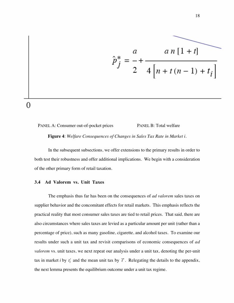
18

PANEL A: Consumer out-of-pocket prices PANEL B: Total welfare

Figure 4: Welfare Consequences of Changes in Sales Tax Rate in Market i.

In the subsequent subsections, we offer extensions to the primary results in order to

both test their robustness and offer additional implications. We begin with a consideration

of the other primary form of retail taxation.

3.4 Ad Valorem vs. Unit Taxes

The emphasis thus far has been on the consequences of ad valorem sales taxes on

supplier behavior and the concomitant effects for retail markets. This emphasis reflects the

practical reality that most consumer sales taxes are tied to retail prices. That said, there are

also circumstances where sales taxes are levied as a particular amount per unit (rather than a

percentage of price), such as many gasoline, cigarette, and alcohol taxes. To examine our

results under such a unit tax and revisit comparisons of economic consequences of ad

valorem vs. unit taxes, we next repeat our analysis under a unit tax, denoting the per-unit

tax in market i by ′ti and the mean unit tax by ′t . Relegating the details to the appendix,

the next lemma presents the equilibrium outcome under a unit tax regime.

19

LEMMA 2. Under unit taxes, the supplier's input price, the firm's production decision, and

its profits are as follows:

′w =12

a − ′t − c + v[ ]; ′qi =14

a − 2 ′ti + ′t − c − v[ ]; and

′Π =14

′ti2

i=1

n∑ +

n

16a2 − 2a ′t − 3 ′t 2 − [c + v][2(a − ′t ) − c − v]( ).

Using the equilibrium outcome in Lemma 2, the next proposition presents the unit

tax analogs to Propositions 2 and 3.

PROPOSITION 8.

(i) An increase in market i 's unit tax rate decreases the supplier's wholesale price, i.e.,d ′w

d ′ti< 0.

(ii) An increase in the unit tax rate in market i increases the firm's profit for

′ti > [a + 3 ′t − c − v] / 4 .

Note from Proposition 8 that the fundamental forces at work under ad valorem

taxes remain in play under unit taxes. That is, by lowering consumer valuation of each

retail unit purchased, unit sales taxes shrink consumer demand and increase the sensitivity

of the retailer's input purchase to the wholesale price. This natural compression of retail

margins, in turn, compels the supplier to cut its chosen wholesale price to ensure sufficient

demand (Proposition 8(i)). Despite unit sales taxes in market i undercutting retail profit in

that market, the retailer gains spillover effects in other markets due to the wholesale price

cut. Provided the other markets present sufficient relative profit potential, this wholesale

price benefit can outweigh the loss of demand in market i, and the retailer can again benefit

from unilateral hikes in tax rates (Proposition 8(ii)).

The natural follow-up question, and one routinely asked, is to consider how

outcomes compare between ad valorem and unit taxes. In particular, suppose each market

20

is characterized by an ad valorem sales tax as in the original model formulation, and market

i shifts from its ad valorem sales tax of ti to unit tax of tiu in such a way as to keep the

consumers in that market unaffected. In our setting, this corresponds to the equilibrium

consumer out-of pocket price in market i remaining unchanged. With consumers in that

market left indifferent by the switch, how is the retail firm affected? The next proposition

demonstrates the subtlety that input market effects bring to the question.

PROPOSITION 9. Consider a shift from an ad valorem sales tax to a unit tax in market i that

results in the same out-of-pocket cost for market i consumers. In this case, denoting the

average tax rates in the other markets by t̂ , i.e., t̂ =1

n −1t j

j=1j≠i

n∑ ,

(i) if the firm insources, it prefers the unit tax; while

(ii) if the firm outsources, it may prefer the ad valorem tax. In particular, for c = v = 0,

the ad valorem tax is preferred for ti > t̃i =−B + B2 − 4AC

2A, where:

A = −4n4[1+ t̂ ]2 − 4[1+ 2t̂ ]2 + 24n[1+ 3t̂ + 2t̂ 2 ]+ 3n3[9 +17t̂ + 8t̂ 2 ]

− n2[44 + 99t̂ + 52t̂ 2 ];

B = 8t̂ [1+ 2t̂ ]2 + 4n4[1+ t̂ ]2[3 + 4t̂ ]− 56nt̂ [1+ 3t̂ + 2t̂ 2 ]

− n3[23 +135t̂ +192t̂ 2 + 80t̂ 3]+ n2[9 +143t̂ + 284t̂ 2 +144t̂ 3]; and

C = −16n4t̂ [1+ t̂ ]3 − 4t̂ 2[1+ 2t̂ ]2 + 32nt̂ 2[1+ 3t̂ + 2t̂ 2 ]

+ 2n3[−1+11t̂ + 60t̂ 2 + 80t̂ 3 + 32t̂ 4 ]− n2[−1+ 6t̂ +100t̂ 2 +192t̂ 3 + 96t̂ 4 ].

Proposition 9(i) confirms the well-known traditional comparison (e.g., Anderson et

al. 2001b). Absent input market effects, ad valorem taxes can achieve the same retail

market equilibrium as unit taxes while shifting more of the surplus away from the retail

firm in favor of the government. The reason for this is that unit taxes add one dimension of

consumer price-sensitivity – each unit costs a fixed amount more for consumers which, in

turn, restricts retail supply. Ad valorem taxes, on the other hand, introduce two

dimensions of consumer price-sensitivity – each unit costs more for consumers which, in

21

turn, restricts retail supply; the restricted retail supply ups retail price which then further

adds to the tax-imposed additional consumer cost. By adding this second dimension of

consumer price-sensitivity, ad valorem taxes add more "punch" to the destruction of retailer

margins.

Proposition 9(ii) confirms that even this standard result can reverse in the presence

of input market considerations. The reasoning for the flip is precisely because of the added

punch ad valorem taxes add to shrinking retailer margins: this rapid shrink in a retailer's

margin leads to more rapid cuts in the wholesale price set by the supplier. That is, denoting

the wholesale price with the unit tax by wu , w∗ < wu . And, when the profit potential in

other markets from these wholesale price cuts is sufficiently large, the input market effect

can outweigh the retail market effect for market i.

The next figure presents a graphical depiction of the underlying differences between

ad valorem and unit taxes in the presence of a strategic supplier.

PANEL A: Wholesale prices PANEL B: Firm profits

Figure 5: Unit Taxes vs. Ad Valorem Taxes.

22

3.5 Competition

The primary analysis centers around a simple supply chain setting of a monopolist

supplier providing inputs to a monopolist retailer in order to highlight the key effects

supply chains introduce to an examination of economic effects of sales taxes. We now

append this primary analysis to consider a competitive retail market (section 3.5.1) and a

competitive wholesale market (section 3.5.2).

3.5.1 COMPETITION IN THE OUTPUT MARKET

To examine if the results herein are robust to retail market competition and to

consider the repercussions of competition in light of reliance on suppliers, consider the

following extension – rather than the firm being a monopolist in each market, it now faces a

(Cournot) competitor who also relies on its own (dedicated) supplier for inputs. Further,

denote consumer demand in market i by p̂i = a − qi − γqRi and p̂Ri = a − qRi − γqi , where

p̂i ( p̂Ri) represents the consumer out-of-pocket price for the firm's (rival's) good in market

i, qi ( qRi) represents the retail quantity provided by the firm (rival) in market i, and γ ,

γ ∈[0,1], reflects the degree of competitive intensity (product substitutability) between the

firm and rival.

In this setting, the relevant condition on consumer demand to ensure interior

solutions is a >2(1+ tmax )(1+ t )

2(1− tmax ) + γti + (4 − γ )t

⎡

⎣⎢

⎤

⎦⎥[c + v]. While the appendix derives the

equilibrium under this modified scenario, the key conclusion, representing the analog to

Proposition 3, is presented in the next Proposition.

23

PROPOSITION 10. Under output market competition,

(i) an increase in sales tax in market i increases the firm's profit for ti > ti*(γ ) , where

ti*(γ ) i s t h e u n i q u e ti -va lue t ha t so lves ti = f (t ;γ ),

f (t ;γ ) = [4 − γ ](6 − γ )(2 − γ )

(1+ t )2 +2[c + v]

a⎛⎝

⎞⎠

2⎡

⎣⎢

⎤

⎦⎥

−1/2

−1.

(ii) the greater the degree of retail competition, the less often the firm benefits from an

increase in sales taxes, i.e., dti

*(γ )dγ

> 0.

Proposition 10(i) confirms that the key conclusions of our primary analysis are

robust in the presence of retail competition ( γ > 0). In other words, it is the supply chain

effects, not the presumed absence of retail competition, that drives our primary results.

Proposition 10(ii) takes the next step to consider how the degree of competition alters this

supply chain relationship. As retail competition increases, a firm's ability to parlay lower

wholesale prices into greater retail profit are limited. As a result, the loss in retail demand

from higher sales taxes becomes (relatively) more prominent, thereby reducing the

circumstances under which firms actually benefit from hikes in tax rates in a market. This

suggests that circumstances under which retailers are less likely to oppose proposals to

increase (or introduce) sales taxes are those in which the retailer has substantial market

power (concentration).

3.5.2 COMPETITION IN THE INPUT MARKET

Continuing the theme of competition, consider the case of nontrivial supply market

competition. To examine varying degrees of supply competition most succinctly, consider

the case of Cournot competition among N suppliers, N ≥ 1 (see, e.g., Arya and Pfeiffer

2012). In this case, the condition for positive equilibrium retail quantities is

24

a >N(1+ tmax )(1+ t )

N − tmax + (N +1)t

⎡

⎣⎢

⎤

⎦⎥[c + v]. Relegating details to the appendix, the next proposition

presents the analog to Proposition 3 in the case of supply market competition.

PROPOSITION 11. Under Cournot competition in the supply market,

(i) an increase in sales tax in market i increases the firm's profit for ti > ti*(N) , where

ti*(N) i s t h e u n i q u e ti -va lue tha t so lves ti = f (t ;N),

f (t ;N) =2N +1

(N +1)2(1+ t )2 +N(c + v)(N +1)a

⎛⎝⎜

⎞⎠⎟

2⎡

⎣⎢⎢

⎤

⎦⎥⎥

−1/2

−1.

(ii) the greater the degree of input market competition, the less often the firm benefits from

an increase in sales taxes, i.e., dti

*(N)dN

> 0.

Proposition 11(i) generalizes the result of Proposition 3 to the case of supplier

competition. The result confirms that it is not a monopolist supplier that matters, but rather

imperfect coordination of the supply chain. Proposition 11(ii), however, confirms that

greater competition does mitigate the supply market effects of sales taxes. As can be

expected, for N = 1, f (t; N) reduces to the cutoff value in Proposition 3. As competition

increases in the supply market, the extent to which sales taxes can cut wholesale prices is

reduced since input market competition already serves to shrink the prevailing wholesale

price. In other words, sales taxes and competition serve as substitutes when it comes to

mitigating double marginalization along the supply chain. As for the limiting case of

N →∞ , this corresponds to the insourcing case since that entails marginal-cost pricing. In

that limiting case, the condition in Proposition 11(i) reduces to ti > f (t; N) =a

c + v−1, a

condition that cannot be jointly satisfied with the nonnegativity condition – with perfect

competition in the supply market, a retail firm can never benefit from a hike in sales tax

rates . Beyond the limiting case, however, the condition for a preference for tax hikes is

non-trivial, i.e., for all finite N, there always exist parameters that satisfy the condition

ti > f (t; N).

25

The next figure provides a pictorial summary of the effects of competition, both in

the retail and supply realms.

PANEL A: Retail competition PANEL B: Wholesale competition

Figure 6: Effects of Competition on Preference for Sales Tax Increase.

4. Implications and Conclusion

While it has long been recognized that consumer-demand effects of retail sales taxes

can present notable economic repercussions, little if any attention has been paid to supply

chain consequences of such taxes. This paper examines such consequences and finds that

sales taxes can have notable effects on supply markets and these effects alter traditional

views of tax policy when (i) suppliers exhibit pricing power and (ii) retail firms operate in

multiple tax jurisdictions.

In particular, we show that increases in sales taxes in one retail market not only

undercut retail demand but also wholesale demand (this despite the fact that wholesale

purchases themselves are not taxed). This reduced wholesale demand compels the supplier

to cut its input price to maintain demand for its goods in the high-tax market. This lower

26

input price, in turn, permits a retailer to provide more and cheaper goods to consumers in

other markets.

The results introduce caveats to the traditional views of sales taxes and offer some

implications for future study. In terms of the former, not only do the results conclude that

the most basic premise of conventional wisdom – that consumers and firms prefer taxes to

be lower – may not always be true, they also suggest that tax jurisdictions may be able to

leverage this to gain support for unilateral shifts in taxes. A key driver of this result arises

when markets are characterized by potential differences in tax rates, as is the case across

states and across sales platforms (in-store vs. online). In that case, attempts to raise tax

rates in one market may actually face limited resistance (and even tacit support) by retailers

due to the spillover effects to the retailer's other markets. Among other things, this may

reflect why retailers have fought aggressively to limit collecting sales/use taxes for online

purchases but show less aggression in fighting local sales tax hikes.

The results also demonstrate that due to supplier pricing effects, welfare is

maximized when tax burdens are shared equally across markets. This suggests that well-

intentioned efforts to target tax breaks to some product or consumer groups may have

deleterious effects because the supply pricing consequences will lead to a counterproductive

shift of resources to particular markets or consumers.

Finally, we note that our results provide some empirical implications for the well-

established streams of literature on tax incidence. In particular, the fundamental question of

whether a tax burden levied at the consumer level will fully be borne by consumers or

whether further retail price hikes will lead the tax to be "overshifted" has been extensively

studied, with mixed empirical evidence. Our results suggest a mitigating factor to

overshifting is the degree to which supply markets are coordinated. A fully coordinated or

highly competitive supply market will favor the overshifting often implied by existing

models. However, our results show that when supply markets exhibit powerful and

strategic suppliers, the imposition of additional tax on consumers may support the notion of

27

"undershifting" thanks to input price cuts; this tension is consistent with the partial tax

shifting observed empirically in some (but not all) retail markets.

Though the focus here is on taxes levied on purchases in particular retail markets,

the results are also suggestive of effects of government subsidies tied to purchases

(negative sales taxes) seen in certain markets. For example, when tax credits are tied to

purchases of specific energy-efficient products, the conventional wisdom is that the boost

in demand will promote energy efficiency. The results here note that the subsidy can also

lead to a concomitant hike in supplier prices and that this price hike may actually raise retail

prices of other products using energy efficient technologies that are not subject to tax

incentives. Thus, while targeted subsidies may boost sales of the energy efficient products

targeted, they can also have the unintended consequence of undercutting sales of other

energy efficient product categories.

Taken one step further, the results also suggest an additional avenue of study: when

government incentives seek to boost demand for socially-beneficial services (e.g., higher

education or medical care), a full understanding of the policy consequences would require

consideration of how strategic input suppliers (in particular, labor), respond to such

consumer incentives. Future study could examine these broader consequences in a model

of labor supply.

28

APPENDIX

Proof of Proposition 1. Under insourcing, the firm's production decision is obtained

by solving the following problem:

Maxq1,...,qn

a − qi

1+ ti− c − v

⎡

⎣⎢

⎤

⎦⎥qi

i=1

n∑ . (A1)

The first-order condition of (A1) yields qi (v) = [1 / 2] a − (1+ ti )(c + v)[ ]. The

non-negativity condition noted in the text implies a > [1+ ti ][c + v] ensuring qi (v) > 0 .

Setting w = v in (2), (3), and (4) yields tax collections, firm profits, and welfare

expressions in the insourcing case. Taking appropriate derivatives then yields:

dΠ(v)dti

= −a2 − [1+ ti ]

2[c + v]2

4[1+ ti ]2 ;

dTi (v)dti

=a2 − [1+ ti ]

2[1+ 2ti ][c + v]2

4[1+ ti ]2 and

dT j (v)

dti= 0 , j ≠ i ;

dp̂i (v)dti

=d[a − qi (v)]

dti=

c + v

2 and

dp̂j (v)

dti=

d[a − qj (v)]

dti= 0; and

dΨ(v)dti

=d [a − qi (v) − c − v]qi (v) + qi

2(v) / 2{ }dti

= −[a − (1− ti )(c + v)][c + v]

4.

Given a > [1+ ti ][c + v], dΠ(v)

dti< 0 ,

dp̂i (v)dti

> 0, and dΨ(v)

dti< 0. The

comparative static on Ti (v) is positive if a

[1+ ti ][c + v]> 1+ 2ti , and negative otherwise.

Proof of Lemma 1. Under outsourcing, solving (A1) with v replaced by w yieldsqi (w) = [1 / 2] a − (1+ ti )(c + w)[ ]. Thus, the supplier's problem is:

Maxw

w − v[ ] qi (w)i=1

n∑ ≡

n

2w − v[ ] a − (1+ t )(c + w)[ ]. (A2)

The first-order condition of (A2) yields w∗ in Lemma 1, and qi∗ = qi (w

∗). Finally,

Π∗ = a − qi

∗

1+ ti− c − w∗⎡

⎣⎢

⎤

⎦⎥qi

∗

i=1

n∑ and Ti

* = tia − qi

∗

1+ ti

⎡

⎣⎢

⎤

⎦⎥qi

∗ . The lower bound on a noted in

text corresponds to qi∗ > 0 for all i .

Proof of Proposition 2. Using w∗ from Lemma 1,

29

dw∗

dti= −

a

2[1+ t ]2dt

dti= −

a

2n[1+ t ]2 < 0.

Proof of Proposition 3. Using Π∗ from Lemma 1,

dΠ∗

dti=

116

a2 −4

[1+ ti ]2 +

3

[1+ t ]2

⎛

⎝⎜

⎞

⎠⎟ + c + v( )2

⎡

⎣⎢⎢

⎤

⎦⎥⎥

and

d2Π∗

dti2 =

a2

84n[1+ t ]3 − 3[1+ ti ]

3

n[1+ ti ]3[1+ t ]3

⎡

⎣⎢

⎤

⎦⎥ . (A3)

Note 4n[1+ t ]3 − 3[1+ ti ]3 > 4n[1+ ti / n]3 − 3[1+ ti ]

3 > 3; the last inequality

follows from the fact that the minimum value of 4n[1+ ti / n]3 − 3[1+ ti ]3 for n ≥ 2 and

0 ≤ ti ≤ 1 is 3 which corresponds to the choice of n = 2 and ti = 1. Thus, from the second

equality in (A3) , Π∗ is convex in ti , i.e., d2Π∗ / dti2 > 0. Given this, dΠ∗ / dti > 0 for

all ti > ti*, where ti

* is the unique solution that solves dΠ∗ / dti = 0. From the first

equality in (A3), dΠ∗ / dti = 0 is equivalent to the condition ti = f (t ) , with f (t ) as noted

in Proposition 3.

Proof of Proposition 4. Using Π∗ from Lemma 1 and, replacing ti by ti + Δ , Δ ≥ 0,

for all i , yields Π∗(Δ) , the firm's profit as a function of Δ :

Π∗(Δ) =14

a2 11+ ti + Δ

⎛

⎝⎜

⎞

⎠⎟

i=1

n∑ −

n

43a2

1+ t + Δ+ [c + v][2a − (1+ t + Δ)(c + v)]

⎛

⎝⎜

⎞

⎠⎟

⎡

⎣⎢⎢

⎤

⎦⎥⎥.

Taking the derivative of the above expression with respect to Δ yields:

dΠ∗(Δ)dti

= −a2

41

1+ ti + Δ

⎛

⎝⎜

⎞

⎠⎟

2

−n

1+ t + Δ( )2i=1

n∑

⎧⎨⎪

⎩⎪

⎫⎬⎪

⎭⎪+

n

41

1+ t + Δ( )2−

c + v

a⎛⎝

⎞⎠

2⎧⎨⎪

⎩⎪

⎫⎬⎪

⎭⎪

⎡

⎣

⎢⎢

⎤

⎦

⎥⎥.

The proof follows from the fact that each term in the { }-brackets is positive as we

next show. The second term in the { }-brackets is positive since the non-negativity

condition on quantities implies a > [1+ t + Δ][c + v]. The firm term in the { }-brackets is

positive if 1+ t + Δ( )2 > n

11+ ti + Δ

⎛

⎝⎜

⎞

⎠⎟

2

i=1

n∑

. This is proved below making use of the facts

that: (i) the arithmetic mean is greater than the harmonic mean for positive data, leading to

the first inequality and (ii) E[xi2 ] > E2[xi ], where xi = 1 / [1+ ti + Δ], giving the second

inequality:

30

1+ t + Δ( )2 > n2

11+ ti + Δi=1

n∑

⎛

⎝⎜

⎞

⎠⎟

2 >n2

n1

1+ ti + Δ

⎛

⎝⎜

⎞

⎠⎟

2

i=1

n∑

=n

11+ ti + Δ

⎛

⎝⎜

⎞

⎠⎟

2

i=1

n∑

.

Proof of Proposition 5. Using T j* , j ≠ i , in (6),

dT j∗

dti=

at j[1+ t j ][a + (1+ t j )(c + v)]

8n[1+ t ]3> 0.

Using Ti* in (6),

d2Ti∗

dti2 = −

c + v[ ] 2a ti (1+ ti ) − n(1+ 2ti )(1+ t ) + n2(1+ t )2{ } + (c + v)n2(1+ t )3[ ]8n2[1+ t ]3

−

a2 3ti (1+ ti )

4 − 2n(1+ ti )3(1+ 2ti )(1+ t ) + n2(1+ t )2(5 + 3ti + 3ti

2 + ti3 + 8t + 4t 2 )[ ]

8n2[1+ ti ]3[1+ t ]4 .

For 0 < ti < 1 and n ≥ 2, the terms ti (1+ ti ) − n(1+ 2ti )(1+ t ) + n2(1+ t )2 > 0 and

3ti (1+ ti )4 − 2n(1+ ti )

3(1+ 2ti )(1+ t ) + n2(1+ t )2(5 + 3ti + 3ti2 + ti

3 + 8t + 4t 2 ) > 0. Thus,

it follows that Ti∗ is concave in ti , i.e., d2Ti

∗ / dti2 < 0. Given concavity, dTi

∗ / dti > 0

for ti < tiT where ti

T is the ti -value that solves dTi∗ / dti = 0 . From Ti

* in (6),

dTi∗

dti=

g(ti ,t )

16n[1+ ti ]2[1+ t ]3

, where g(ti ,t ) is noted in Proposition 5. Thus, tiT is the

unique ti -value that solves g(ti ,t ) = 0 .

Proof of Proposition 6. Using Lemma 1,

dp̂i∗

dti=

d[a − qi*]

dti=

a[n −1+ nt − ti ]

4n[1+ t ]2 +c + v

4> 0 and

dp̂j∗

dti=

d[a − qj*]

dti= −

a[1+ t j ]

4n[1+ t ]2 < 0.

Proof of Proposition 7. Since Ψ∗ = a − qi*[ ]qi

* − vqi* − cqi

* +[qi

*]2

2

⎛

⎝⎜

⎞

⎠⎟

i=1

n∑ , from

Lemma 1,

Ψ∗ =na2[7 +14t + 7t 2 − σt

2 ]

32[1+ t ]2 −

n c + v[ ] 2a 7 +10t + 3t 2 + σt

2{ } − (c + v)(1+ t ) 7 + 6t − t 2 − σt2{ }[ ]

32[1+ t ].

31

Using the above,

d2Ψ∗

dti2 = −

a2[n(1+ t )2 + 2t + 3t 2 −1− 4ti (1+ t ) + 3σt2 ]

16n[1+ t ]4 −

c + v[ ] 2a n(1+ t )2 + t 2 −1− 2ti (1+ t ) + σt

2{ } + n(c + v)(1+ t )3[ ]16n[1+ t ]3

< 0.

The above inequality follows from the fact that, given the lower bound on a (i.e.,

the non-negativity condition on quantities), t > ti / n , σt2 > [ti − t ]2 / n, and n ≥ 2, the

numerator of each of the two terms on the right-hand-side of d2Ψ∗ / dti2 is positive, i.e.,

n(1+ t )2 + 2t + 3t 2 −1− 4ti (1+ t ) + 3σt2 > 0 and

2a n(1+ t )2 + t 2 −1− 2ti (1+ t ) + σt2{ } + n(c + v)(1+ t )3 > 0 .

Given concavity, dΨ∗ / dti > 0 for ti < tiΨ where ti

Ψ is the ti -value that solves

dΨ∗ / dti = 0 . From Ψ∗ above, dΨ∗

dti=

h(ti ,t ,σt2 )

16[1+ t ]3, where h(ti ,t ,σt

2 ) is noted in

Proposition 7. Thus, tiΨ is the unique ti -value that solves h(ti ,t ,σt

2 ) = 0 .

Proof of Lemma 2. Under unit taxes, the firm chooses quantities by solving the

following problem:

Maxq1,...,qn

a − qi − c − w − ′ti[ ]qii=1

n∑ .

The first-order condition of the above yields qi (w) = [1 / 2] a − c − ′ti − w[ ]. Thus,

the supplier's problem is:

Maxw

w − v[ ] qi (w)i=1

n∑ ≡

n

2w − v[ ] a − c − ′t − w[ ].

The solution to the supplier's problem yields ′w ; and, so, ′qi = qi ( ′w ) ; under this

solution the firm's profit equals ′Π .

Proof of Proposition 8. Using the firm profit expressions from Lemma 2, the results

follows from the following comparative statics:

d ′Πd ′ti

=18

4 ′ti − a − 3 ′t + c + v[ ] and d ′′Πi

d ′′ti= −

116

a − c − v[ ]2 < 0.

Proof of Proposition 9. Consider the case of insourcing. Lemma 1 provides the

quantities under sales tax. With w = v , the proof of Lemma 2 provides the quantities under

32

unit tax. For the consumers in market i to be indifferent, the consumer price (and, hence,

the quantity) in market i should be equal, i.e.,

a − [1+ ti ][c + v]2

=a − ti

u − c − v

2⇒ ti

u = ti[c + v].

The firm's profit under sales tax is Π(v); with the shift to unit tax in market i and

tiu = ti[c + v], the firm's profit is Πu(v), where:

Π(v) =[a − (1+ t j )(c + v)]2

4[1+ t j ]j=1

n∑ and

Πu(v) =[a − (1+ ti )(c + v)]2

4+

[a − (1+ t j )(c + v)]2

4[1+ t j ]j=1j≠i

n∑ .

Thus, Πu(v) − Π(v) =ti[a − (1+ ti )(c + v)]2

4[1+ ti ]> 0, proving part (i). Under

outsourcing, with the shift to unit tax in market i , the firm's problem is:

Maxq1,...,qn

a − qi − c − w − tiu[ ]qi +

a − qj

1+ t j− c − w

⎡

⎣⎢⎢

⎤

⎦⎥⎥qj

j=1j≠i

n∑ . (A4)

The first-order condition of (A4) yields:

qi (w) = [1 / 2][a − c − tiu − w] and qj (w) = [1 / 2][a − (1+ t j )(c + w)]. (A5)

Using (A5), the supplier's problem is:

Maxw

w − v[ ] [qi (w) + qj (w)j=1j≠i

n∑ ] ≡

12

w − v[ ] a − tiu − c − w + [n −1][a − (1+ t̂ )(c + w)][ ].

The above problem yields:

wu =12

an − tiu

n(1+ t ) − ti− c + v

⎡

⎣⎢

⎤

⎦⎥. (A6)

For the consumers in market i to be indifferent, the quantity in market i should be equal

under the unit tax and the sales tax, i.e.,

qi (wu ) = qi

∗ ⇔ [1 / 2][a − c − tiu − wu ] =

a

2−

[1+ ti ][a + (1+ t )(c + v)]4[1+ t ]

.

Solving the above for tiu yields:

33

tiu =

ti2n(1+ t ) − 2ti −1

⎡

⎣⎢

⎤

⎦⎥

a[n(1+ t ) −1− ti ]1+ t

+ [n(1+ t ) − ti ][c + v]⎡⎣⎢

⎤⎦⎥. (A7)

Using quantities from (A5), wholesale price from (A6), and the unit tax rate from

(A7) in (A4) yields firm profit of:

Πu =14

a − tiu − c − wu[ ]2 + 1

4a2 1

1+ t j

⎛

⎝⎜

⎞

⎠⎟

j=1j≠i

n∑ − 2a[n −1][c + wu ]+ [n(1+ t ) −1− ti ][c + wu ]2

⎡

⎣

⎢⎢⎢

⎤

⎦

⎥⎥⎥

.

Using Πu from above and Π∗ from Lemma 1,

Π∗ − Πu

c=v=0=

a2ti[Ati2 + Bti + C]

16[1+ ti ][n(1+ t ) + ti − t ]2[1+ 2t − 2n(1+ t )]2 , where (A8)

A = −4n4[1+ t̂ ]2 − 4[1+ 2t̂ ]2 + 24n[1+ 3t̂ + 2t̂ 2 ]+ 3n3[9 +17t̂ + 8t̂ 2 ]

− n2[44 + 99t̂ + 52t̂ 2 ];

B = 8t̂ [1+ 2t̂ ]2 + 4n4[1+ t̂ ]2[3 + 4t̂ ]− 56nt̂ [1+ 3t̂ + 2t̂ 2 ]

− n3[23 +135t̂ +192t̂ 2 + 80t̂ 3]+ n2[9 +143t̂ + 284t̂ 2 +144t̂ 3]; and

C = −16n4t̂ [1+ t̂ ]3 − 4t̂ 2[1+ 2t̂ ]2 + 32nt̂ 2[1+ 3t̂ + 2t̂ 2 ]

+ 2n3[−1+11t̂ + 60t̂ 2 + 80t̂ 3 + 32t̂ 4 ]− n2[−1+ 6t̂ +100t̂ 2 +192t̂ 3 + 96t̂ 4 ].

From (A8), Π∗ − Πu

c=v=0> 0 if and only if Ati

2 + Bti + C > 0. At ti = 0,

Ati2 + Bti + C = C < 0. Also,

d[Ati2 + Bti + C]

dti= 2Ati + B > 0. Thus, the t̃i cutoff

corresponds to the ti -value in [0,1] that solves the quadratic Ati2 + Bti + C = 0 . This root

is noted in part (ii).

Proof of Proposition 10. Under (Cournot) retail competition, the firm and the rival

solve the following problems, respectively:

Maxq1,...,qn

a − qi − γqRi

1+ ti− c − w

⎡

⎣⎢

⎤

⎦⎥qi

i=1

n∑ and Max

qR1,...,qRn

a − qRi − γqi

1+ ti− c − wR

⎡

⎣⎢

⎤

⎦⎥qRi

i=1

n∑ . (A9)

Simultaneously solving the first-order conditions of the above problems yields:

qi (w,wR;γ ) =1

2 + γa − (1+ ti )(c +

2w − γwR

2 − γ⎡

⎣⎢

⎤

⎦⎥ and

34

qRi (w,wR;γ ) =1

2 + γa − (1+ ti )(c +

2wR − γw

2 − γ⎡

⎣⎢

⎤

⎦⎥ . (A10)

Given (A10), the firm's supplier chooses w to maximize w − v[ ]qi (w,wR;γ )i=1

n∑ ,

while the rival's supplier sets wR to maximize w − v[ ]qRi (w,wR;γ )i=1

n∑ . Jointly solving the

two first-order conditions yields the wholesale prices w∗(γ ) and wR∗ (γ ); using these in

(A10) yields the quantities qi∗(γ ) and qRi

∗ (γ ); and using these prices and quantities in (A9)

gives firm profit of Π∗(γ ). These expressions are presented below:

w∗(γ ) = wR∗ (γ ) =

14 − γ

a[2 − γ ]1+ t

+ 2v − c[2 − γ ]⎡⎣⎢

⎤⎦⎥;

qi∗(γ ) = qRi

∗ (γ ) =1

[4 − γ ][2 + γ ]a[2(1− ti ) + γti + (4 − γ )t ]

1+ t− 2[1+ ti ][c + v]⎡

⎣⎢⎤⎦⎥; and

Π∗(γ ) =1

[2 + γ ]2 a2 11+ ti

⎛

⎝⎜

⎞

⎠⎟

i=1

n∑ −

n

[4 − γ ]2a2[6 − γ ][2 − γ ]

1+ t+ 4[c + v][2a − (1+ t )(c + v)]

⎛

⎝⎜

⎞

⎠⎟

⎡

⎣⎢⎢

⎤

⎦⎥⎥.

From the expression for quantities above, the non-negativity condition in the retail

competition setting is a >2(1+ tmax )(1+ t )

2(1− tmax ) + γti + (4 − γ )t

⎡

⎣⎢

⎤

⎦⎥[c + v]. Also, from the above,

dΠ∗(γ )dti

=1

[2 + γ ]2 a2 −1

[1+ ti ]2 +

[6 − γ ][2 − γ ]

[4 − γ ]2[1+ t ]2

⎛

⎝⎜

⎞

⎠⎟ +

4 c + v( )2

[4 − γ ]2

⎡

⎣⎢⎢

⎤

⎦⎥⎥. (A11)

Some tedious calculation confirm that d2Π∗(γ )

dti2 > 0 . Thus, for ti > ti

*(γ ) , dΠ∗(γ )

dti> 0 ,

where ti*(γ ) is the ti -value that solves

dΠ∗(γ )dti

= 0. From (A11), dΠ∗(γ )

dti= 0 is

equivalent to the condition ti = f (t ;γ ), where f (t ;γ ) is as in part (i). Turning to part (ii),

dti*(γ )dγ

=∂f (t ;γ )

∂t

∂t

∂γ+∂f (t ;γ )∂γ

=∂f (t ;γ )

∂t

1n

dti*(γ )dγ

+∂f (t ;γ )∂γ

⇒dti

*(γ )dγ

1−1n

∂f (t ;γ )∂t

⎡⎣⎢

⎤⎦⎥=∂f (t ;γ )∂γ

. (A12)

Using f (t ;γ ) from part (i),

∂f (t ;γ )∂γ

=4a[1+ t ] a2 − (1+ t )2(c + v)2[ ]

a2(12 − 8k + k2 ) + 4(1+ t )2(c + v)2[ ]3/2 > 0 and

35

1n

∂f (t ;γ )∂t

=[6 − γ ][2 − γ ][1+ f (t ;γ )]3

n[1+ t ]3[4 − γ ]2 < 1. (A13)

From (A12) and (A13), dti

*(γ )dγ

> 0.

Proof of Proposition 11. As noted in the proof of Lemma 1,qi (w) = [1 / 2] a − (1+ ti )(c + w)[ ]. Let yj , j = 1,..., N , denote the quantity supplied by

the jth supplier. Equating total demand with total supply,

qi (w)i=1

n∑ = yj

j=1

N∑ ⇒ w =

an − cn[1+ t ]− 2 yjj=1

N∑

n[1+ t ]. (A14)

Given (A14), and taking supply of other suppliers as given under (Cournot) input

market competition, supplier k solves:

Maxyk

an − cn[1+ t ]− 2 yj − 2ykj=1j≠k

N∑

n[1+ t ]− v

⎡

⎣

⎢⎢⎢⎢⎢⎢

⎤

⎦

⎥⎥⎥⎥⎥⎥

yk , k = 1,..., N . (A15)

Jointly solving the first-order conditions of the problem in (A15) yields yk∗(N);

using this in (A14) yields w∗(N); qi (w∗(N)) is then denoted qi

∗(N); and firm profit under

these choices of quantity and input price is denoted Π∗(N):

yj∗(N) =

n[a − (1+ t )(c + v)]2[N +1]

; w∗(N) =1

N +1a

1+ t− c + Nv⎡

⎣⎢⎤⎦⎥

;

qi∗(N) =

12(N +1)

a[N − ti + (N +1)t ]1+ t

− N(1+ ti )(c + v)⎡⎣⎢

⎤⎦⎥; and

Π∗(N) =a N − ti + [N +1]t( ) − N 1+ ti( ) 1+ t( ) c + v( )[ ]2

4[N +1]2[1+ t ]2[1+ ti ]

⎧⎨⎪

⎩⎪

⎫⎬⎪

⎭⎪i=1

n∑ .

From the expression for quantities above, the non-negativity condition in the supplier

competition setting is a >N(1+ tmax )(1+ t )

N − tmax + (N +1)t

⎡

⎣⎢

⎤

⎦⎥[c + v]. Also, from the above,

36

dΠ∗(N)dti

=14

a2 −1

[1+ ti ]2 +

2N +1

[N +1]2[1+ t ]2

⎛

⎝⎜

⎞

⎠⎟ +

N2 c + v( )2

[N +1]2

⎡

⎣⎢⎢

⎤

⎦⎥⎥. (A16)

It can be easily confirmed that d2Π∗(N)

dti2 > 0 . Thus, for ti > ti

*(N) , dΠ∗(N)

dti> 0 , where

ti*(N) is the ti -value that solves

dΠ∗(N)dti

= 0. From (A16), dΠ∗(N)

dti= 0 is equivalent to

the condition ti = f (t ;N), where f (t ;N) is as in part (i). Turning to part (ii),

dti*(N)dN

=∂f (t ;N)

∂t

∂t

∂N+∂f (t ;N)∂N

=∂f (t ;N)

∂t

1n

dti*(N)dN

+∂f (t ;N)∂N

⇒dti

*(N)dN

1−1n

∂f (t ;N)∂t

⎡⎣⎢

⎤⎦⎥=∂f (t ;N)∂N

. (A17)

Using f (t ;N) from part (i),

∂f (t ;N)∂N

=Na[1+ t ] a2 − (1+ t )2(c + v)2[ ]

a2(2N +1) + N2(1+ t )2(c + v)2[ ]3/2 > 0 and

1n

∂f (t ;N)∂t

=[2N +1][1+ f (t ;N)]3

n[1+ t ]3[N +1]2 < 1. (A18)

From (A17) and (A18), dti

*(N)dN

> 0.

37

REFERENCES

Anderson, S., de Palma, A., Kreider, B. 2001a. Tax Incidence in Differentiated Product

Oligopoly. Journal of Public Economics 81, 173-192.

Anderson, S., de Palma, A., Kreider, B. 2001b. The Efficiency of Indirect Taxes under

Imperfect Competition. Journal of Public Economics 81, 231-251.

Arya, A., Mittendorf, B. 2007. Interacting Supply Chain Distortions: The Pricing of

Internal Transfers and External Procurement. The Accounting Review 82, 551-580.

Arya, A., Mittendorf, B. 2011. Supply Chains and Segment Profitability: How Input

Pricing Creates a Latent Cross-Segment Subsidy. The Accounting Review 86, 805-

824.

Arya, A., Pfeiffer, T. 2012. Manufacturer-Retailer Negotiations in the Presence of an

Oligopolistic Input Market. Production and Operations Management 21, 534-546.

Baugh, B., Ben-David, I., Park, H. 2014. The "Amazon Tax": Empirical Evidence from

Amazon and Main Street Retailers. Working Paper, The Ohio State University.

Besley, T., Rosen, H. 1999. Sales Taxes and Prices: An Empirical Analysis. National Tax

Journal 52, 157-178.

Cachon, G., Lariviere, M. 2005. Supply Chain Coordination with Revenue-Sharing

Contracts: Strengths and Limitations. Management Science 51, 30-44.

Goolsbee, A., Zittrain, J. 1999. Evaluating the Costs and Benefits of Taxing Internet

Commerce. National Tax Journal 52, 413-428.

Hamilton, S. 2008. Excise Taxes with Multiproduct Transactions. American Economic

Review 99, 458-471.

Hoopes, J., Thornock, J., Williams, B. 2014. Is Sales Tax Avoidance a Competitive

Advantage. Working Paper, The Ohio State University.

Katz, M. L. 1989. Vertical Contractual Relations. Handbook of Industrial Organization 1,

655-721.

Lariviere, M. 1999. Supply Chain Contracting and Coordination with Stochastic Demand.

In S. Tayur, R. Ganeshan, and M. Magazine (eds.), Quantitative Models for Supply

Chain Management. Kluwer.

Marion, J., Muehlegger, E. 2011. Fuel Tax Incidence and Supply Conditions. Journal of

Public Economics 95, 1202-1212.

38

Pal, D., Sappington, D., Tang, Y. 2012. Sabotaging Cost Containment. Journal of

Regulatory Economics 41, 293-314.

Pasternack, B. 1985. Optimal Pricing and Return Policies for Perishable Commodities.

Marketing Science 4, 166-176.

Poterba, J. 1996. Retail Price Reactions to Changes in State and Local Sales Taxes.

National Tax Journal 49, 165-176.

Sappington, D., Weisman, D. 2005. Self-Sabotage. Journal of Regulatory Economics 27,

155-175.

Spengler, J. J. 1950. Vertical Integration and Antitrust Policy. The Journal of Political

Economy 58, 347-352.

Tsay, A. 1999. The Quantity Flexibility Contract and Supplier-Customer Incentives.

Management Science 45, 1339-1358.

Tsay, A., Agrawal, N. 2004. Modeling Conflict and Coordination in Multi-Channel

Distribution Systems: A Review. International Series in Operations Research and

Management Science, 557-680.