Prepared for submission to JCAP

Conservative cosmology: combiningdata with allowance for unknownsystematics

Jose Luis Bernala,b John A. Peacockc

aICC, University of Barcelona, IEEC-UB, Martı i Franques, 1, E08028 Barcelona, SpainbDept. de Fısica Quantica i Astrofısica, Universitat de Barcelona, Martı i Franques 1, E08028Barcelona, SpaincInstitute for Astronomy, University of Edinburgh, Royal Observatory, Blackford Hill, Edinburgh,EH9 3HJ, UK

E-mail: joseluis.bernal@icc.ub.edu, jap@roe.ac.uk

Abstract. When combining data sets to perform parameter inference, the results will be unreliable ifthere are unknown systematics in data or models. Here we introduce a flexible methodology, BACCUS:BAyesian Conservative Constraints and Unknown Systematics, which deals in a conservative waywith the problem of data combination, for any degree of tension between experiments. We introduceparameters that describe a bias in each model parameter for each class of experiments. A conservativeposterior for the model parameters is then obtained by marginalization both over these unknown shiftsand over the width of their prior. We contrast this approach with an existing method in which eachindividual likelihood is scaled, comparing the performance of each approach and their combination inapplication to some idealized models. Using only these rescaling is not a suitable approach for thecurrent observational situation, in which internal null tests of the errors are passed, and yet differentexperiments prefer models that are in poor agreement. The possible existence of large shift systematicscannot be constrained with a small number of data sets, leading to extended tails on the conservativeposterior distributions. We illustrate our method with the case of the H0 tension between resultsfrom the cosmic distance ladder and physical measurements that rely on the standard cosmologicalmodel.

arX

iv:1

803.

0447

0v2

[as

tro-

ph.C

O]

3 J

ul 2

018

Contents

1 Introduction 1

2 Overview of assumptions and methodology 2

3 Application to illustrative examples 43.1 Shift parameters in the one-parameter Gaussian case 43.2 Contrasting shift and rescaling parameters 73.3 Examples with multiple parameters 7

4 Applications to cosmology: H0 94.1 Data and modelling 94.2 Results 11

5 Summary and discussion 14

1 Introduction

For two decades or more, the standard Λ-Cold Dark Matter (ΛCDM) cosmological model has suc-ceeded astonishingly well in matching new astronomical observations, and its parameters are preciselyconstrained (e.g. [1–3]). However, more recent work has persistently revealed tensions between highand low redshift observables. In the case of the Hubble constant, H0, the best direct measurementusing cepheids and supernovae type Ia [4] is in 3.4σ tension with the value inferred assuming ΛCDMusing Planck observations [1]. Planck and weak lensing surveys both measure the normalization ofdensity fluctuations via the combination Ω0.5

m σ8, and their estimates were claimed to be in 2.3σ ten-sion by the KiDS collaboration [5] – although recent results from DES are less discrepant [6]. Theseinconsistencies are not currently definitive (e.g. [7]), but they raise the concern that something couldbe missing in our current cosmological understanding. It could be that the ΛCDM model needsextending, but it could also be that the existing experimental results suffer from unaccounted-forsystematics or underestimated errors.

When inconsistent data are combined naively, it is well understood that the results risk beinginaccurate and that formal errors may be unrealistically small. For this reason, much emphasis isplaced on tests that can be used to assess the consistency between two data sets (e.g. [8–10]). Werefer the interested reader to [11, 12] for more methodologies but also for a comprehensive comparisonbetween different measures of discordance. Another approach is the posterior predictive distribution,which is the sampling distribution for new data given existing data and a model, as used in e.g., [13].However, these methods are not really helpful in cases of mild tension, where a subjective binarydecision is required as to whether or not a genuine inconsistency exists.

Unknown systematics can be modelled as the combination of two distinct types. Type 1 sys-tematics affect the random scatter in the measurements (and therefore the size of the errors in aparameterised model), but do not change the maximum-posterior values for the parameters of themodel. In contrast, type 2 systematics offset the best-fitting parameters without altering the randomerrors; they are completely equivalent to shifts in the parameters of the model without modifying theshape of the posterior of each parameter. While the former are commonly detectable through internalevidence, the latter are more dangerous and they can only reveal themselves when independent exper-iments are compared. Much of our discussion will focus on this class of systematic. With a detailedunderstanding of a given experiment, one could do better than this simple classification; but here weare trying to capture ‘unknown unknowns’ that have evaded the existing modelling of systematics,and so the focus must be on the general character of these additional systematics.

Taking all this into account, there is a need for a general conservative approach to the combinationof data. This method should allow for possible unknown systematics of both kinds and it should permit

– 1 –

the combination of data sets in tension with an agnostic perspective. Such a method will inevitablyyield uncertainties in the inferred parameters that are larger than in the conventional approach, buthaving realistic uncertainties is important if we are to establish any credible claims for the detectionof new physics.

The desired method can be built using a hierarchical approach. Hierarchical schemes havebeen used widely in cosmology, e.g. to model in more detail the dependence of the parameters oneach measurement in the case of H0 and the cosmic distance ladder [14], or the cosmic shear powerspectrum [15]. While the extra parameters often model physical quantities, our application simplyrequires empirical nuisance parameters. The introduction of extra parameters to deal with datacombination was first introduced in the pioneering discussion of [16]. A more general formulation wasprovided by [17] and refined in [18] (H02 hereinafter). This work assigns a free weight to each data set,rescaling the logarithm of each individual likelihood (which is equivalent to rescaling the errors of eachexperiment if the likelihood is Gaussian), in order to achieve an overall reduced χ2 close to unity. TheH02 method yields meaningful constraints when combining data sets affected by type 1 errors, and itdetects the presence of the errors by comparing the relative evidences of the conventional combinationof data and their approach. However, this method is not appropriate for obtaining reliable constraintsin the presence of type 2 systematics, where we might find several experiments that all have reducedχ2 values of unity, but with respect to different best-fitting models. H02 do not make our distinctionbetween different types of systematics, but in fact they do show an example where one of the datasets has a systematic type 2 shift (see Figures 3 & 4 of H02). Although their method does detect thepresence of the systematic, we do not feel that it gives a satisfactory posterior in this case, for reasonsdiscussed below in section 3.2.

Here we present a method called BACCUS1, BAyesian Conservative Constraints and UnknownSystematics, which is designed to deal with systematics of both types. Rather than weighting eachdata set, the optimal way to account for type 2 systematics is to consider the possibility that theparameters preferred by each experiment are offset from the true values. Therefore, extra parametersshift the model parameters when computing each individual likelihood, and marginalized posteriorsof the model parameters will account for the possible existence of systematics in a consistent way.Moreover, studying the marginalized posteriors of these new parameters can reveal which experimentsare most strongly affected by systematics.

This paper is structured as follows. In Section 2, we introduce our method and its key underlyingassumptions. In Section 3, we consider a number of illustrative examples of data sets constructed toexhibit both concordance and discordance, contrasting the results from our approach with those ofH02. We then apply our method to a genuine cosmological problem, the tension in H0, in Section 4.Finally, a summary and some general discussion of the results can be found in Section 5. We use theMonte Carlo sampler emcee [19] in all the cases where Monte Carlo Markov Chains are employed.

2 Overview of assumptions and methodology

We begin by listing the key assumptions that underlie our statistical approach to the problem ofunknown systematics. Firstly, we will group all codependent experiments in different classes, andconsider each of them independent from the others. For example, observations performed with thesame telescope or analyzed employing the same pipeline or model assumptions will be considered in thesame class, since all the really dangerous systematics would be in common. Then, our fundamentalassumption regarding systematics will be that a experiment belonging to each of these classes isequally likely to commit an error of a given magnitude, and that these errors will be randomly andindependently drawn from some prior distribution. Attempts have been made to allow for dependencebetween data sets when introducing scaling parameters as in H02 (see [20]). We believe that a similarextension of our approach should be possible, but we will not pursue this complication here.

With this preamble, we can now present the formalism to be used. Consider a model M , pa-rameterised by a set of model parameters, θ (we will refer to M(θ) as θ for simplicity), which are

1A python package implementing is publicly available in https://github.com/jl-bernal/BACCUS.

– 2 –

to be constrained by several data sets, D. The corresponding posterior, P (θ|D), and the likelihood,P (D|θ), are related by the Bayes theorem:

P (θ|D) =P (θ)P (D|θ)

P (D), (2.1)

where P (θ) is the prior. We will consider flat priors in what follows and concentrate on the likelihood,unless otherwise stated. For parameter inference, we can drop the normalization without loss ofgenerality.

We can account for the presence of the two types of systematics in the data by introducingnew parameters. For type 2 systematics, the best fit values of the parameters for each experiment,θi, may be offset from the true value by some amount. We introduce a shift parameter, ∆i

θj, for

each parameter θj and class i of experiments. For type 1 systematics, we follow H02 and introduce arescaling parameter αi which weights the logarithm of the likelihood of each class of experiments; if thelikelihood is Gaussian, this is equivalent to rescaling each individual χ2 and therefore the covariance.Considering ni data points for the class of experiments i, the likelihood is now:

P(θ,α, ∆θ|D) ∝∏i

αni/2i exp

[−αi

2

(χ2

bf,i + ∆χ2i (θ + ∆i

θ − θi))], (2.2)

where χ2bf is the minimum χ2, corresponding to the best-fit value of θ, θ. Here, we use the notation

∆θ to indicate the vector of shift parameters for each parameter of the model. There is a differentvector of this sort for every class of experiments, indexed by i.

For rescaling parameters, H02 argue that the prior should be taken as:

P(αi) = exp[−αi] (2.3)

so that the mean value of αi over the prior is unity, i.e. experiments estimate the size of theirrandom errors correctly on average. One might quarrel with this and suspect that underestimationof errors could be more common, but we will retain the H02 choice; this does not affect the resultssignificantly. In realistic cases where the number of degrees of freedom is large and null tests are passedso that χ2

bf,i ' n, the scope for rescaling the errors will be small and αi will be forced to be close tounity. For the prior on shift parameters, we choose a zero-mean Gaussian with a different unknownstandard deviation determined by σθj , corresponding to each parameter θj and common to all classesof experiments. Furthermore, it is easy to imagine systematics that might shift several parameters ina correlated way, so that the prior on the shifts should involve a full covariance matrix, Σ∆, containingthe variances, σ2

θj , in the diagonal and off-diagonal terms obtained with the correlations ρj1,j2 for eachpair of shifts (Σj1,j2 = ρj1,j2σθj1σθj2 ). Thus the assumed prior on the shifts is:

P(∆θ|σθ,ρ) ∝N∏i

|Σ∆|−1/2exp

[−1

2∆iθ

TΣ−1

∆ ∆iθ

]. (2.4)

We now need to specify the hyperpriors for the covariance matrix of the shifts, Σ∆. Our philos-ophy here is to seek an uninformative hyperprior: it is safer to allow the data to limit the degree ofpossible systematic shifts, rather than imposing a constraining prior that risks forcing the shifts tobe unrealistically small.

Different options of priors for covariance matrices are discussed by e.g. [21]. In order to ensureindependence among variances and correlations, we use a separation strategy, applying different priorsto variances and correlations (e.g. [22]). A covariance matrix can be expressed as Σ = SRS, withS being a diagonal matrix with Sjj = σθj and R, the correlation matrix, with Rii = 1 and Rij =ρij . As hyperprior for each of the covariances we choose a lognormal distribution (log σ = N(b, ξ),where N(b, ξ) is a Gaussian distribution in log σ with mean value b and variance ξ). In the case ofthe correlation matrix, we use the LKJ distribution [23] as hyperprior, which depends only on theparameter η: for η = 1, it is an uniform prior over all correlation matrices of a given order; for η > 1,lower absolute correlations are favoured (and vice versa for η < 1). The parameters b, ξ and η can be

– 3 –

chosen to suit the needs of the specific problem. We prefer to be as agnostic as possible, so we willchoose η = 1 and b and ξ such as the hyperprior of each covariance is broad enough to not to forcethe shifts to be small.

The final posterior can be marginalized over all added parameters, leaving the conservativedistribution of the model parameters θ, that is the main aim of this work. This immediately providesa striking insight: a single experiment gives no information whatsoever. It is only when we have severalexperiments that the possibility of large σθ starts to become constrained (so that the ∆θ cannotbe too large). In the case of consistent data, as the shifts are drawn from a Gaussian distribution,only small shifts are favoured (as the individual likelihoods would not overlap otherwise). If, on theother hand, only two data sets are available and there is a tension between them regarding someparameter θj , the prior width σθj could be of the order of such tension, but much larger values willbe disfavoured.

However, an alternative would be to obtain the marginalized posteriors of ∆θ. This tells usthe likely range of shifts that each data set needs for each parameter, so that unusually discrepantexperiments can be identified by the system. As we will see in examples below, this automaticallyresults in their contribution to the final posterior being downweighted. If one class of experimentshas shifts that are far beyond all others, this might give an objective reason to repeat the analysiswithout it, but generally we prefer not to take this approach: judging whether an offset is significantenough to merit exclusion is a somewhat arbitrary decision, and is complicated in a multidimensionalparameter space. Our formalism automatically downweights data sets as their degree of inconsistencygrows, and this seems sufficient.

3 Application to illustrative examples

3.1 Shift parameters in the one-parameter Gaussian case

In order to exhibit all the features of our method more clearly, we first apply the formalism to thesimple model in which there is only one parameter (θ = a) and the probability density functions(PDFs) of a for the N individual experiments are Gaussian. In this case, we can rewrite Equation2.2 as:

P(a,α,∆a, σa|D) ∝N∏i

αni/2i exp

[−1

2αi(χ2i,bf + ∆χ2

i (a+ ∆ia))]. (3.1)

We apply the prior for rescaling parameters (Equation 2.3) and marginalize over each αi to obtainthe marginalized posterior for a single class of experiments:

Pi(a,∆ia, σa|Di) ∝

(∆χ2

i (a+ ∆ia) + 2

)−(ni/2+1). (3.2)

For large ni, χ2i+2 ' χ2

i , and the right hand side of Equation 3.2 is proportional to exp[−(∆χ2i /2)(ni/χ

2i,bf)],

which in effect instructs us to rescale parameter uncertainties according to (χ2ν,i)

1/2, where χ2ν,i is the

reduced χ2i for the class of experiments i. But it can be assumed that experiments will pursue inter-

nal null tests to the point where χ2ν ' 1; thus in practice rescaling parameters can do little to erase

tensions.Assuming hereafter that experimenters will achieve χν = 1 exactly, we can now focus on the

novel feature of our approach, which is the introduction of shift parameters. Then, the posterior canbe written as

P(a,∆a, σa|D) ∝N∏i

σ−1a exp

[−1

2

ni∑k=1

((yki (a+ ∆i

a)−Dki

)2σki

2

)+

∆ia

2

2σ2a

], (3.3)

where yki (x) is the theoretical prediction to fit to the measurement Dki of the class of experiments i,

with error σki . Note that the width of the prior for the shifts, σa, is the same for all data sets, by

– 4 –

0.0

0.5

1.0

/m

axN = 2 N = 4

4 2 0 2 4a

0.0

0.5

1.0

/m

ax

N = 2

4 2 0 2 4a

N = 4

Individual posteriors Conventional combination Accounting for systematics

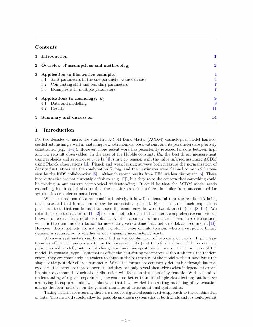
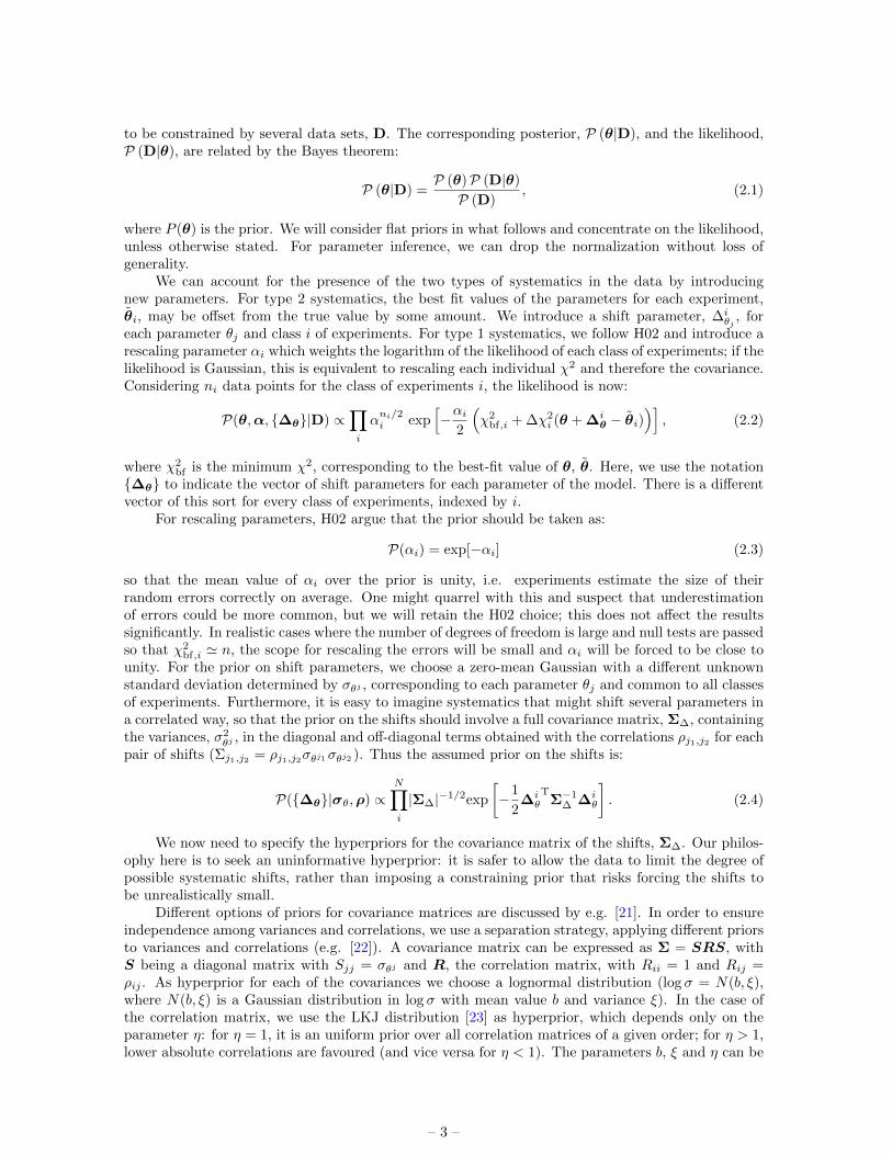
Figure 1. Comparison of the results obtained using shift parameters and the conventional approach tocombining data sets in a model with only one parameter, a, and N data sets whose individual posteriors areGaussians. We show individual posteriors in black, the posteriors obtained with the conventional approachin orange and the posterior obtained with our approach, in purple. The dependence of the posterior on thenumber of data sets for the exactly consistent case is shown in the top panels, while strongly inconsistentcases are shown in the bottom panels.

assumption. Marginalizing over the shifts, then the posterior of each class of experiments is:

Pi(a, σa|D) ∝ni∏k=1

(σki2

+ σ2a)−1/2 exp

−1

2

(yki (a)−Dk

i

)2(σki

2+ σ2

a

)2

. (3.4)

Therefore, our method applied to a model with only one parameter and Gaussian likelihoods reducesto the convolution of the original posteriors with a Gaussian of width σa.

Finally, we need to marginalize over σa. Consider for example a hyperprior wide enough to beapproximated as uniform in σa, and suppose that all the N data sets agree on ai = 0 and all theerrors, σki = σi, are identical. Then we can derive the marginalized posterior in the limit of small andlarge a:

P(a|D) ∝

1− exp

[(N−1)a2

2σ2i

], for a 1

a1−N , for a 1(3.5)

For values of a close to ai the posterior presents a Gaussian core, whose width is σi/√N − 1, in

contrast with the conventional σi/√N from averaging compatible data. For values of a very far

from ai, the posterior has non-Gaussian power-law tails. For N = 2 these are so severe that thedistribution cannot be normalized, so in fact three measurements is the minimum requirement toobtain well-defined posteriors. As will be discussed in Section 5, one can avoid such divergence bychoosing harder priors on ∆i

a or σa, but we prefer to be as agnostic as possible. Nonetheless, these‘fat tails’ on the posterior are less of an issue as N increases. These two aspects of compatible datacan be appreciated in the top panels of Figure 1. The message here is relatively optimistic: providedwe have a number of compatible data sets, the conservative posterior is not greatly different from theconventional one.

Alternatively, we can consider an example of strongly incompatible data. Let theN data sets havenegligible σi and suppose the corresponding ai are disposed symmetrically about a = 0 with spacing ε,e.g. a = (−ε, 0,+ε) for N = 3. This gives a marginalized posterior that depends on N . For example,the tails follow a power law: P(a|D) ∝ (1 + 4a2/ε2)−1/2 for N = 2, P (a|D) ∝ (1 + 3a2/2ε2)−1 for

– 5 –

0.0

0.5

1.0/

max N = 4a)

N = 8b)

0.0

0.5

1.0

/m

ax

c)N = 4

a

N = 8d)

4 2 0 2 4a

0.0

0.5

1.0

/m

ax N = 8e)

4 2 0 2 4a

f)N = 8

Individual posteriors Conventional combination Accounting for systematics

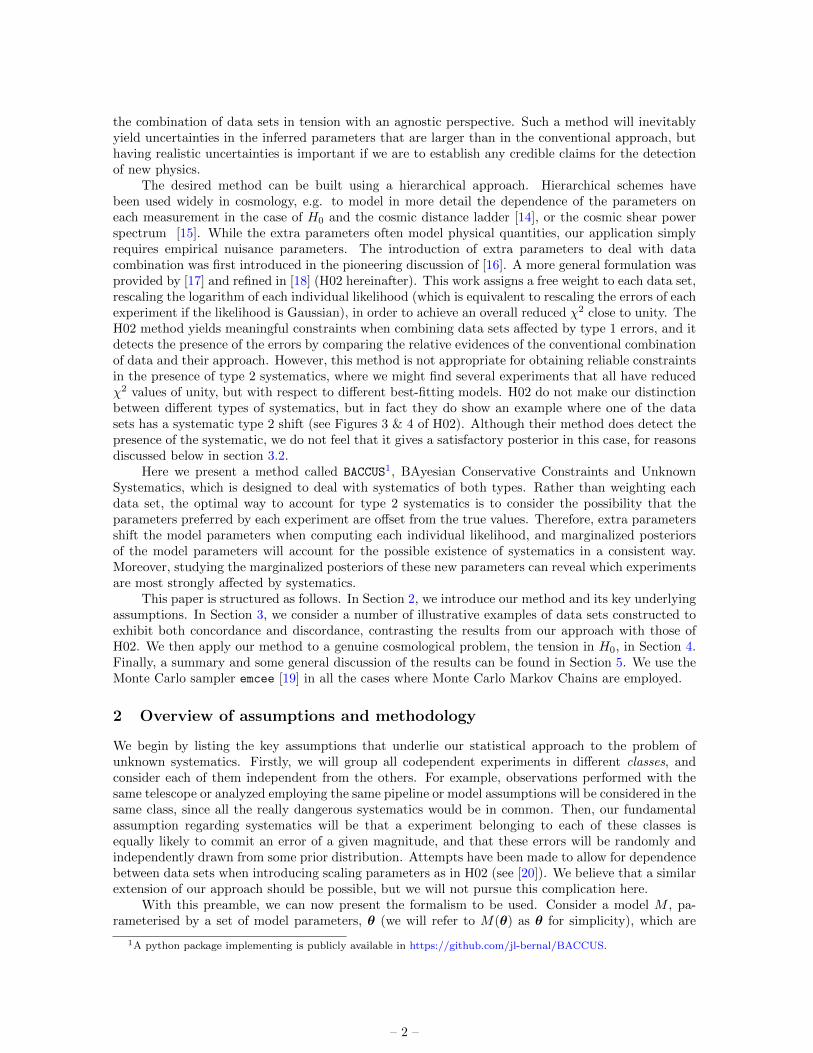
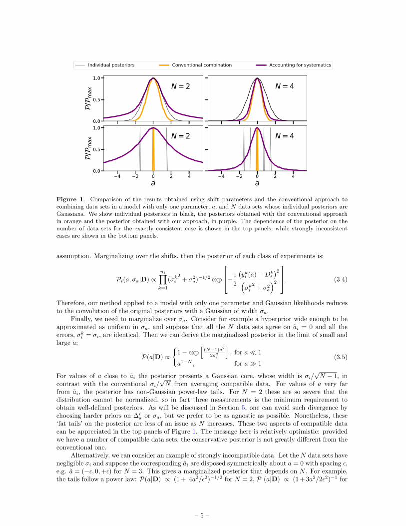
Figure 2. The same as Figure 1, but considering cases in which all the data sets are consistent (panels a andb), only one is discrepant with the rest (panels c and d), eight data sets with scatter larger than the errors(panel e) and eight data sets with random values of the best fit and errors (panel f).

N = 3, etc., with an asymptotic dependence of (a/ε)1−N for N 1. So, as in the previous case, theposterior cannot be normalized if N = 2, but it rapidly tends to a Gaussian for large N . This caseis shown in the bottom panels of Figure 1. The appearance of these extended tails on the posterioris a characteristic result of our method, and seems inevitable if one is unwilling in advance to limitthe size of possible shift systematics. The power-law form depends in detail on the hyperprior, but ifwe altered this by some power of σa, the result would be a different power-law form for the ‘fat tails’still with the generic non-Gaussinianity.

We also show in Figure 2 some more realistic examples, starting with mock consistent data thatare drawn from a Gaussian using the assumed errors (rather than a = 0), but then forcing one or moreof these measurements to be discrepant. As with the simple a = 0 example, we see that the resultsfor several consistent data sets approach the conventional analysis for larger N (panels a and b). Butwhen there is a single discrepant data set, the posterior is much broader than in the conventionalcase (panel c). Nevertheless, as the number of consistent data sets increases, the posterior shrinks tothe point where it is only modestly broader than the conventional distribution, and where the singleoutlying measurement is clearly identified as discrepant (panel d). Thus our prior on the shifts, inwhich all measurements are assumed equally likely to be in error, does not prevent the identificationof a case where there is a single rogue measurement. However, these examples do emphasize thedesirability of having as many distinct classes of measurement as possible, even though this maymean resorting to measurements where the individual uncertainties are larger. Additional coarseinformation can play an important role in limiting the tails on the posterior, especially in cases wherethere are discordant data sets (see panel d). Finally, we also show examples where the scatter of the

– 6 –

individual best-fit is larger than the individual uncertainties of the data sets, so the size of the shiftsare larger and our posterior is broader than the one obtained with conventional approach (panel e),and a case with several inconsistent measurements (with best-fit and errors distributed randomly),for which our posterior is centred close to 0 with a width set by the empirical distribution of the data(panel f).

3.2 Contrasting shift and rescaling parameters

If we ignore the constraints on αi and consider only the relative likelihoods (with width of the distri-bution determined by σi), then there is an illuminating parallel between the effects of rescaling andshift parameters. Compare Equation 3.4, where all α have been already marginalized over (P1), withH02’s method (P2):

P1 ∝∏i

(σ2a + σ2

i )−1/2 exp

[−1

2

∑i

(a− ai)2

σ2a + σ2

i

]; P2 ∝

∏i

α1/2i σ−1

i exp

[−1

2

∑i

αi(a− ai)2

σ2i

],

(3.6)

these two expressions are clearly the same if αi =(1 + σ2

a/σ2i

)−1. However, there is a critical differ-

ence: while there is an αi for each class of experiments, we only consider a single σa, which participatesin the prior for all the shift parameters of all classes of experiments.

On the other hand, if different σθj for each data sets were to be used, this would be equivalentto a double use of rescaling parameters. Furthermore, in the case of having several experiments withinconsistent results, the posterior using only rescaling parameters would be a multimodal distributionpeaked at the points corresponding to the individual posteriors, as seen in Figures 3 & 4 of H02. Wefeel that this is not a satisfactory outcome: it seems dangerously optimistic to believe that one outof a flawed set of experiments can be perfect when there is evidence that the majority of experimentsare incorrect. Our aim should be to set conservative constraints, in which all experiments have todemonstrate empirically that they are not flawed (i.e. ‘guilty until proved innocent’).

3.3 Examples with multiple parameters

The approach to models with multiple parameters differs conceptually from the one-parameter case:there are several families of shifts, ∆θ, with their corresponding covariance matrix. A convenientsimple illustration is provided by the example chosen by H02: consider data sets sampled from differentstraight lines. Thus, the model under consideration is y = mx + c, where y & x are the informationgiven by the data and m & c are the parameters to constrain.

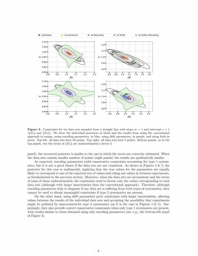
We consider three different straight lines for which we sample the data, Di: D1 and D2 ≡ m =c = 1; D3 ≡ m = 0, c = 1.5; and D4 ≡ m = c = 0.7. For all Di, we consider three inde-pendent data sets (so N = 6 when combining i.e., D1 and D2) and assume σy = 0.1 for every datapoint. We combine D1 with D2 in Figure 3, with D3 in Figure 4, and with D4 in Figure 5.Note the change of scale in each panel. In all cases, we study four situations corresponding to thecombination of: all data sets with 50 or 5 points and errors correctly estimated or underestimated bya factor 5 (only in data sets from D2, D3 or D4). We use lognormal priors with b = −2 andξ = 16 both for σm and σc, and a LKJ distribution with η = 1 as the shifts hyperprior. We showthe individual posteriors of each data set in black; the results using the conventional approach inorange; the constraints using only rescaling parameters in blue; using only shift parameters in purple;and using both in green. The occasional noisy shape of the latter is due to the numerical complexityof sampling the parameter space using rescaling and shifts. Generally, in this case the uncertaintiesare somewhat larger than in the case of using only shifts, except when individual errors are poorlyestimated and the credible regions are much larger. This is because rescaling parameters gain a largeweight in the analysis in order to recover a sensible χ2

ν,i, which permits shifts that are too large forthe corresponding prior (given that the corresponding likelihood is downweighted by small values ofαi). This can be seen comparing green and purple contours in the bottom panels of Figures 3, 4 & 5.

As can be seen in Figure 3, if the data sets are consistent and the errors are correctly estimated(top left panel), rescaling parameters have rather little effect on the final posterior. This supports ourargument in Equation 3.2 and below. On the other hand, when errors are underestimated (bottom left

– 7 –

0.8 0.9 1.0 1.1 1.2 1.3m

0.80

0.85

0.90

0.95

1.00

1.05

1.10c

0.6 0.8 1.0 1.2 1.4 1.6 1.8m

0.6

0.8

1.0

1.2

1.4

c

0.8 0.9 1.0 1.1 1.2 1.3m

0.80

0.85

0.90

0.95

1.00

1.05

1.10

c

0.6 0.8 1.0 1.2 1.4 1.6m

0.6

0.8

1.0

1.2

1.4

c

Individual Conventional w/ Rescaling w/ Shifts w/ Shifts+Rescaling

Figure 3. Constraints for six data sets sampled from a straight line with slope m = 1 and intercept c = 1(D1 and D2). We show the individual posteriors in black and the results from using the conventionalapproach in orange, using rescaling parameters, in blue, using shift parameters, in purple, and using both ingreen. Top left: all data sets have 50 points. Top right: all data sets have 5 points. Bottom panels: as in thetop panels, but the errors of D2 are underestimated a factor 5.

panel), the recovered posterior is similar to the one in which the errors are correctly estimated. Whenthe data sets contain smaller number of points (right panels) the results are qualitatively similar.

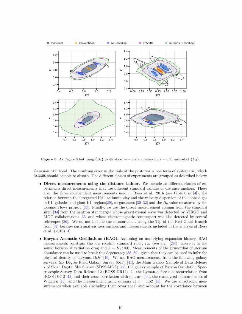
As expected, rescaling parameters yield conservative constraints accounting for type 1 system-atics, but it is not a good choice if the data sets are not consistent. As shown in Figures 4 & 5, theposterior for this case is multimodal, implying that the true values for the parameters are equallylikely to correspond to one of the reported sets of values and ruling out values in between experiments,as foreshadowed in the previous section. Moreover, when the data sets are inconsistent and the errorsof some of them underestimated, the constraints tend to favour only the values corresponding to suchdata sets (although with larger uncertainties than the conventional approach). Therefore, althoughrescaling parameters help to diagnose if any data set is suffering from both types of systematics, theycannot be used to obtain meaningful constraints if type 2 systematics are present.

On the other hand, using shift parameters gives constraints with larger uncertainties, allowingvalues between the results of the individual data sets and accepting the possibility that experimentsmight be polluted by unaccounted-for type 2 systematics (as it is the case in Figures 4 & 5). Sur-prisingly, they also provide correct conservative constraints when only type 1 systematics are present,with results similar to those obtained using only rescaling parameters (see, e.g., the bottom left panelof Figure 3).

– 8 –

0.5 0.0 0.5 1.0 1.5m

0.8

1.0

1.2

1.4

1.6

1.8c

0.5 0.0 0.5 1.0 1.5m

0.8

1.0

1.2

1.4

1.6

1.8

c

0.5 0.0 0.5 1.0 1.5m

0.8

1.0

1.2

1.4

1.6

1.8

c

0.5 0.0 0.5 1.0 1.5m

0.8

1.0

1.2

1.4

1.6

1.8

c

Individual Conventional w/ Rescaling w/ Shifts w/ Shifts+Rescaling

Figure 4. As Figure 3 but using D3 (with slope m = 0 and intercept c = 1.5) instead of D2.

4 Applications to cosmology: H0

In order to illustrate how our method performs in a problem of real interest, we apply it to thetensions in H0. This tension has been studied from different perspectives in the literature. One ofthe options is to perform an independent analysis of the measurements to check for systematics ina concrete constraint, e.g., by including rescaling parameters to consider type 1 systematics in eachmeasurement used to constrain H0 [24] or using a hierarchical analysis to model in more detail all theprobability distribution functions [14]. Another possibility is to consider that this tension is a hintof new physics, rather than a product of unaccounted-for systematics, and therefore explore if othercosmological models ease it or if model independent approaches result in constraints that differ fromthe expectations of ΛCDM (see [25] and references therein).

Here we propose a third way. We consider all the existing independent constraints of H0 from lowredshift observations and apply BACCUS to combine them and obtain a conservative joint constraintof H0, accounting for any possible scale or shift systematic in each class of experiments (groupedas described in Section 4.1). We use only low redshift observations in order to have a consensusconservative constraint to confront with early Universe constraints from CMB observations. Weassume a ΛCDM background expansion and use the cosmic distance ladder as in [26–28].

4.1 Data and modelling

In this section we describe the data included in the analysis. As discussed in Section 3.1, the sizeof the uncertainties using BACCUS are smaller for a larger number of classes of experiments, even ifthe individual errors are larger. Therefore, we include all independent constraints on H0 from lowredshift observations available, independent of the size of their error bars. In principle, we should usethe exact posterior reported by each experiment, but these are not always easily available. Therefore,we use the reported 68% credible limits in the case of the direct measurements of H0, assuming a

– 9 –

0.4 0.6 0.8 1.0 1.2m

0.4

0.6

0.8

1.0

1.2c

0.00 0.25 0.50 0.75 1.00 1.25 1.50m

0.4

0.6

0.8

1.0

1.2

1.4

c

0.4 0.6 0.8 1.0 1.2 1.4m

0.4

0.6

0.8

1.0

1.2

1.4

c

0.4 0.6 0.8 1.0 1.2 1.4m

0.4

0.6

0.8

1.0

1.2

1.4

c

Individual Conventional w/ Rescaling w/ Shifts w/ Shifts+Rescaling

Figure 5. As Figure 3 but using D4 (with slope m = 0.7 and intercept c = 0.7) instead of D2.

Gaussian likelihood. The resulting error in the tails of the posterior is one form of systematic, whichBACCUS should be able to absorb. The different classes of experiments are grouped as described below:

• Direct measurements using the distance ladder. We include as different classes of ex-periments direct measurements that use different standard candles or distance anchors. Theseare: the three independent measurements used in Riess et al. 2016 (see table 6 in [4]), therelation between the integrated Hβ line luminosity and the velocity dispersion of the ionized gasin HII galaxies and giant HII regions[29], megamasers [30–32] and the H0 value measured by theCosmic Flows project [33]. Finally, we use the direct measurement coming from the standardsiren [34] from the neutron star merger whose gravitational wave was detected by VIRGO andLIGO collaborations [35] and whose electromagnetic counterpart was also detected by severaltelescopes [36]. We do not include the measurement using the Tip of the Red Giant Branchfrom [37] because such analysis uses anchors and measurements included in the analysis of Riesset al. (2016) [4].

• Baryon Acoustic Oscillations (BAO). Assuming an underlying expansion history, BAOmeasurements constrain the low redshift standard ruler, rsh (see e.g. [28]), where rs is thesound horizon at radiation drag and h = H0/100. Measurements of the primordial deuteriumabundance can be used to break this degeneracy [38, 39], given that they can be used to infer thephysical density of baryons, Ωbh

2 [40]. We use BAO measurements from the following galaxysurveys: Six Degree Field Galaxy Survey (6dF) [41], the Main Galaxy Sample of Data Release7 of Sloan Digital Sky Survey (SDSS-MGS) [42], the galaxy sample of Baryon Oscillation Spec-troscopic Survey Data Release 12 (BOSS DR12) [2], the Lyman-α forest autocorrelation fromBOSS DR12 [43] and their cross correlation with quasars [44], the reanalysed measurements ofWiggleZ [45], and the measurement using quasars at z = 1.52 [46]. We use anisotropic mea-surements when available (including their covariance) and account for the covariance between

– 10 –

the different redshift bins within the same survey when needed. We consider BOSS DR12 andWiggleZ measurements as independent because the overlap of both surveys is very small, hencetheir correlation (always below 4%) can be neglected [47, 48]. For our analysis, we considerobservations of different surveys or tracers (i.e., the autocorrelation of the Lyman-α forest andits cross correlation with quasars are subject to different systematics) as different classes ofexperiments.

• Time delay distances. Using the time delays from the different images of strong lensedquasars it is possible to obtain a good constraint on H0 by using the time delay distance if anexpansion history is assumed. We use the three measurements of the H0LiCOW project [49] asa single class of experiment

• Cosmic clocks. Differential ages of old elliptical galaxies provide estimate of the inverse of theHubble parameter, H(z)−1 [50]. We use a compilation of cosmic clocks measurements includingthe measurement of [51], which extends the prior compilation to include both a fine samplingat 0.38 < z < 0.48 using BOSS Data Release 9, and the redshift range up to z ∼ 2. As allcosmic clock measurements have been obtained from the same group using similar analyses, weconsider the whole compilation as a single class of experiment.

• Supernovae Type Ia. As we want to focus mostly on H0, we use the Joint Light curve Analysis(JLA) of Supernovae Type Ia [3] as a single class of experiment to constrain the unnormalizedexpansion history E(z) = H(z)/H0, hence tighter constraints on the matter density parameter,ΩM , are obtained.

We do not consider the assumption of a ΛCDM-like expansion history (which connects BAO,time delay distances, cosmic clocks and supernovae) as a source of systematic errors which couplesdifferent class of experiments (since it affects each observable in a different way). Therefore, we canneglect any correlation among these four probes. In order to interpret the above experiments, weneed a model that contains three free parameters: H0, Ωch

2, and Ωbh2. Ωbh

2 will only be constrainedby a prior coming from [40] and, together with Ωch

2 and H0, allows us to compute rs and break thedegeneracy between H0 and rs in BAO measurements. As we focus on H0 and variations in Ωbh

2

do not affect E(z) significantly, we do not apply any shift to Ωbh2. We compute a grid of values of

100× rsh for different values of H0, Ωch2 and Ωbh

2 using the public Boltzmann code CLASS [52, 53]before running the analysis and interpolate the values at each step of the MCMC to obtain rs in arapid manner2.

4.2 Results

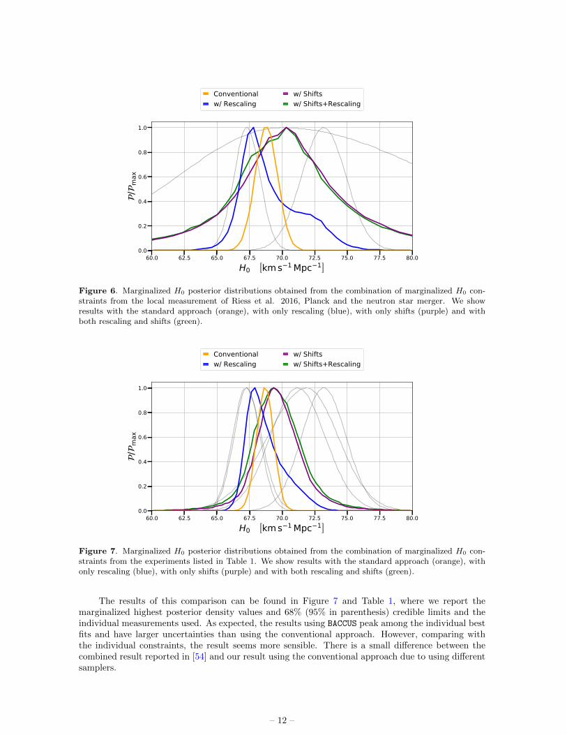
In this section we show the results using BACCUS when addressing the tension in H0. We comparethem with the results obtained using the conventional approach and the methodology introduced inH02. First, we consider marginalized measurements of H0. Ideally, we would apply BACCUS to Riess etal. 2016 and Planck measurements. However, as stated in Section 2, this method can not be appliedto only two measurements. Thus, we use the independent and much broader measurement comingfrom the neutron star merger [34] in order to constrain the tails of the final posterior. These resultscan be found in Figure 6. Even with the inclusion of a third measurement, the tails of the posteriorwhen shift parameters are added are still too large and therefore the conservative constraints are veryweek (due to the low number of experiments included). On the other hand, adding only rescalingparameters results in a bimodal distribution. In order to obtain relevant conservative constraints,more observations need to be included in the analysis.

As the next step, we perform an analysis with more data and compare the results of the differentmethodologies to the combination of the data listed in Table 1, as recently used in [54]. Sincemarginalized constraints in clear tension are combined, this is a case where BACCUS is clearly necessary.We use the lognormal hyperprior with b = −2 and ξ = 16 for the hyperprior of variance of the shiftsin both cases.

2We make a grid for 100 × rsh in order to minimize the error in the interpolation (. 0.1%). This grid is availableupon request.

– 11 –

60.0 62.5 65.0 67.5 70.0 72.5 75.0 77.5 80.0H0 [km s 1 Mpc 1]

0.0

0.2

0.4

0.6

0.8

1.0/

max

Conventionalw/ Rescaling

w/ Shiftsw/ Shifts+Rescaling

Figure 6. Marginalized H0 posterior distributions obtained from the combination of marginalized H0 con-straints from the local measurement of Riess et al. 2016, Planck and the neutron star merger. We showresults with the standard approach (orange), with only rescaling (blue), with only shifts (purple) and withboth rescaling and shifts (green).

60.0 62.5 65.0 67.5 70.0 72.5 75.0 77.5 80.0H0 [km s 1 Mpc 1]

0.0

0.2

0.4

0.6

0.8

1.0

/m

ax

Conventionalw/ Rescaling

w/ Shiftsw/ Shifts+Rescaling

Figure 7. Marginalized H0 posterior distributions obtained from the combination of marginalized H0 con-straints from the experiments listed in Table 1. We show results with the standard approach (orange), withonly rescaling (blue), with only shifts (purple) and with both rescaling and shifts (green).

The results of this comparison can be found in Figure 7 and Table 1, where we report themarginalized highest posterior density values and 68% (95% in parenthesis) credible limits and theindividual measurements used. As expected, the results using BACCUS peak among the individual bestfits and have larger uncertainties than using the conventional approach. However, comparing withthe individual constraints, the result seems more sensible. There is a small difference between thecombined result reported in [54] and our result using the conventional approach due to using differentsamplers.

– 12 –

Experiment/Approach H0 ( km s−1Mpc−1)

Individual Measurements

DES[54] 67.2+1.2−1.0

Planck [1] 67.3± 1.0

SPTpol [55] 71.2± 2.1

H0LiCOW [49] 71.9+2.4−3.0

Riess et al. 2016 [4] 73.2± 1.7

This work

Conventional combination 68.7± 0.6(±1.2)

Rescaling param. 67.8+1.8−0.6(+4.1

−1.3)

Shift param. 69.5+1.7−1.4(+4.7

−3.4)

Shift + rescaling param. 69.4+2.1−1.4(+4.9

−3.8)

Table 1. Individual marginalized constraints on H0 combined to evaluate the performance of our methodin a real one dimensional problem. In the bottom part, we report highest posterior density values and 68%(95% in parenthesis) credible limits obtained combining the individual measurement using different kind ofparameters.

Approach H0 ( km s−1Mpc−1) ΩM

Conventional combination 70.15+0.5−0.6(+1.3

−1.4) 0.32± 0.01(±0.03)

Rescaling param. 69.4± 0.7(±1.5) 0.32± 0.01(±0.03)

Shift param. (only H0) 70.6+0.8−1.1(+1.9

−2.3) 0.31±−0.02(±0.04)

Shift (only H0) + rescaling param. 70.5+0.9−1.3(+2.6

−3.1) 0.31±−0.02(+0.04−0.05)

Shift param. (H0 & ΩM ) 71.7+0.8−1.2(+2.0

−2.8) 0.33± 0.04(+0.09−0.07)

Shift (H0 & ΩM ) + rescaling param. 71.0+1.8−0.9(+3.6

−5.4) 0.33+0.02−0.04(+0.12

−0.14)

Table 2. Highest posterior density values and 68% (95% in parenthesis) credible level marginalized constraintsof H0 and ΩM obtained using the data and methodology described in Section 4.1.

We now apply our method to the data described in Section 4.1 to obtain conservative limits onH0 using all the available independent low redshift observations. Regarding the introduction of shiftparameters, we consider two cases. In the first case (shown in Figure 8) we only use them on H0, ∆H .On the other hand, in the second case (shown in Figure 9) we also use them on Ωch

2, ∆Ω. In bothcases, rescaling parameters are applied to every class of experiments and we use the same parametersas in the previous case for the hyperprior for σH and a lognormal distribution with b = −4 and ξ = 9as the hyperprior for σΩ. We use η = 1 for the LKJ hyperprior of the correlation. Marginalizedcredible limits from both cases can be found in Table 2.

As there is no inconsistency in ΩM among the experiments (given that most of the constraintsare very weak) the only effect of including ∆Ω in the marginalized constraints in ΩM is to broadenthe posteriors. In contrast, including ∆H shifts the peak of the H0 marginalized posterior. Whilethe tightest individual constraints correspond to low values of H0 (BAO and cosmic clocks), BACCUSfavours slightly larger values than the conventional approach (which stays in the middle of the tension,as expected). These effects are larger when we include ∆Ω, given that there is more freedom in theparameter space. On the other hand, as BAO and cosmic clocks are the largest data sets, the analysiswith only rescaling parameters prefers a lower H0. Nonetheless, as the constraints weaken when

– 13 –

64 66 68 70 72 74 76H0 [km s 1 Mpc 1]

0.20

0.25

0.30

0.35

0.40

M

64 66 68 70 72 74 76

0.0

0.2

0.4

0.6

0.8

1.0

0.0 0.2 0.4 0.6 0.8 1.0

0.20

0.25

0.30

0.35

0.40

Conventionalw/ Rescaling

w/ Shiftsw/ Shifts+Rescaling

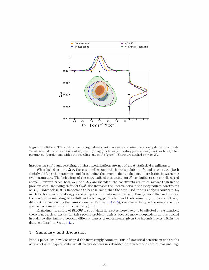
Figure 8. 68% and 95% credible level marginalized constraints on the H0-ΩM plane using different methods.We show results with the standard approach (orange), with only rescaling parameters (blue), with only shiftparameters (purple) and with both rescaling and shifts (green). Shifts are applied only to H0.

introducing shifts and rescaling, all these modifications are not of great statistical significance.When including only ∆H , there is an effect on both the constraints on H0 and also on ΩM (both

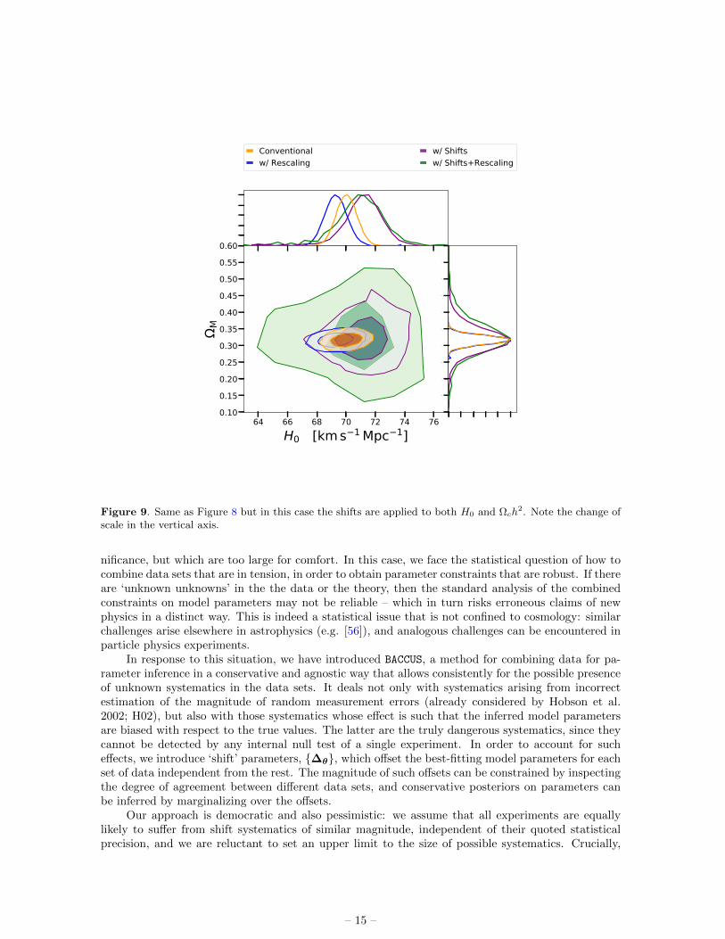
slightly shifting the maximum and broadening the errors), due to the small correlation between thetwo parameters. The behaviour of the marginalized constraints on H0 is similar to the one discussedabove. However, when both ∆H and ∆Ω are included, the constraints are much weaker than in theprevious case. Including shifts for Ωch

2 also increases the uncertainties in the marginalized constraintson H0. Nonetheless, it is important to bear in mind that the data used in this analysis constrain H0

much better than they do ΩM , even using the conventional approach. Finally, note that in this casethe constraints including both shift and rescaling parameters and those using only shifts are not verydifferent (in contrast to the cases showed in Figures 3, 4 & 5), since here the type 1 systematic errorsare well accounted for and individual χ2

ν ' 1.Regarding the ability of BACCUS to spot which data set is more likely to be affected by systematics,

there is not a clear answer for this specific problem. This is because more independent data is neededin order to discriminate between different classes of experiments, given the inconsistencies within thedata sets listed in Section 4.1.

5 Summary and discussion

In this paper, we have considered the increasingly common issue of statistical tensions in the resultsof cosmological experiments: small inconsistencies in estimated parameters that are of marginal sig-

– 14 –

64 66 68 70 72 74 76H0 [km s 1 Mpc 1]

0.100.150.200.250.300.350.400.450.500.550.60

M

64 66 68 70 72 74 76

0.0

0.2

0.4

0.6

0.8

1.0

0.0 0.2 0.4 0.6 0.8 1.0

0.10

0.15

0.20

0.25

0.30

0.35

0.40

0.45

0.50

0.55

0.60

Conventionalw/ Rescaling

w/ Shiftsw/ Shifts+Rescaling

Figure 9. Same as Figure 8 but in this case the shifts are applied to both H0 and Ωch2. Note the change of

scale in the vertical axis.

nificance, but which are too large for comfort. In this case, we face the statistical question of how tocombine data sets that are in tension, in order to obtain parameter constraints that are robust. If thereare ‘unknown unknowns’ in the the data or the theory, then the standard analysis of the combinedconstraints on model parameters may not be reliable – which in turn risks erroneous claims of newphysics in a distinct way. This is indeed a statistical issue that is not confined to cosmology: similarchallenges arise elsewhere in astrophysics (e.g. [56]), and analogous challenges can be encountered inparticle physics experiments.

In response to this situation, we have introduced BACCUS, a method for combining data for pa-rameter inference in a conservative and agnostic way that allows consistently for the possible presenceof unknown systematics in the data sets. It deals not only with systematics arising from incorrectestimation of the magnitude of random measurement errors (already considered by Hobson et al.2002; H02), but also with those systematics whose effect is such that the inferred model parametersare biased with respect to the true values. The latter are the truly dangerous systematics, since theycannot be detected by any internal null test of a single experiment. In order to account for sucheffects, we introduce ‘shift’ parameters, ∆θ, which offset the best-fitting model parameters for eachset of data independent from the rest. The magnitude of such offsets can be constrained by inspectingthe degree of agreement between different data sets, and conservative posteriors on parameters canbe inferred by marginalizing over the offsets.

Our approach is democratic and also pessimistic: we assume that all experiments are equallylikely to suffer from shift systematics of similar magnitude, independent of their quoted statisticalprecision, and we are reluctant to set an upper limit to the size of possible systematics. Crucially,

– 15 –

therefore, the prior for the shifts should take no account of the size of the reported random errors, sinceshift systematics by definition cannot be diagnosed internally to an experiment, however precise it maybe. In practice, we assume that the shifts have a Gaussian distribution, with a prior characterised bysome unknown covariance matrix. We adopt a separation strategy to address the hyperprior for thiscovariance, using the LKJ distribution for the correlations and independent lognormal distributionsfor the standard deviations. We recommend agnostic wide hyperpriors, preferring to see explicitlyhow data can rein in the possibility of arbitrarily large systematics.

For each data set, the shift parameters are assumed to be drawn independently from the sameprior. But this assumption is not valid when considering independent experiments that use thesame technique, since they may well all suffer from systematics that are common to that method.Therefore data should first be combined into different classes of experiments before applying ourmethod. In practice, however, a single experiment may use a number of methods that are substantiallyindependent (e.g. the use of lensing correlations and angular clustering by DES). In that case, ourapproach can be similarly applied to obtain conservative constraints and assess internal consistencyof the various sub-methods.

Because it is common for joint posterior distributions to display approximate degeneracies be-tween some parameters, a systematic that affects one parameter may induce an important shift inothers. For example, in Figure 8 the probability density function of ΩM changes due to ∆H . Forcomplicated posteriors, it is therefore better in principle to use our approach at the level of the anal-ysis of the data (where all the model parameters are varied), rather than constructing marginalizedconstraints on a single parameter of interest and only then considering systematics.

These assumptions could be varied: in some cases there could be enough evidence to considercertain experiments more reliable than others, so that the prior for the shifts will not be universal.But recalling the discussion in 3.1 concerning the use of different shift priors for each data sets, a wayto proceed might be to rescale σθj only for certain data sets (those more trusted), but then to use thesame prior for all data sets after rescaling. If we consider the data sets Di′ to be more reliable thanthe rest, the final prior should be

P(∆a|σa) ∝ 1

σN−1a

exp

−1

2

N∑i 6=i′

(∆ia/σa)2

1

σa/βexp

[−1

2(∆i′

a /(σa/β))2

], (5.1)

where we consider the case with only one parameter a for clarity and β is a constant > 1.Another possibility is to weaken the assumption that arbitrarily bad shift systematics are possible.

One can achieve this either by imposing explicit limits so that the shifts never take values beyondthe chosen bound, or by altering the prior on the shift parameters, making it narrower. Althoughthe methodology is sufficiently flexible to accommodate such customizations, we have preferred tokeep the assumptions as few and simple as possible. As we have seen, large shifts are automaticallydisfavoured as the number of concordant data sets rises, and this seems a better way to achieve theoutcome.

It is also possible to ascertain if a single experiment is affected by atypically large shifts, byinspecting the marginalized posteriors for the shifts applicable to each dataset. A straightforwardoption now is to compute the relative Bayesian evidence between the models with and without shifts,telling us how strongly we need to include them, as done in H02. But this procedure needs care:consider a model with many parameters but only one, θj , strongly affected by type 2 systematics.In that case, the evidence ratio will favour the model without shifts, those not affecting θj are notnecessary. Therefore, the ideal procedure is to check the evidence ratio between models with differentsets of families of shifts, although this is computationally demanding.

After applying our method to some simple example models and comparing it with the scalingof reported errors as advocated by H02, we have applied it to a real case in cosmology: the tensionin H0. In general, H0 values obtained in this way are larger than either those from the conventionalapproach, or the combination using the approach of H02. However, as our conservative uncertaintiesare larger there is no tension when compared with the CMB value inferred assuming ΛCDM. We havefocused on the application to parameter inference by shifting the model parameters for each data set.

– 16 –

However, it is also possible to apply the same approach to each individual measurement of a data set,in the manner that rescaling parameters were used by [24].

We may expect that the issues explored here will continue to generate debate in the future.Next-generation surveys will witness improvements of an order of magnitude in precision, yieldingstatistical errors that are smaller than currently known systematics. Great efforts will be investedin refining methods for treating these known problems, but the smaller the statistical errors become,the more we risk falling victim to unknown systematics. In the analysis presented here, we haveshown how allowance can be made for these, in order to yield error bounds on model parameters thatare conservative. We can hardly claim our method to be perfect: there is always the possibility ofglobal errors in basic assumptions that will be in common between apparently independent methods.Even so, we have shown that realistic credibility intervals can be much broader than the formal onesderived using standard methods. But we would not want to end with a too pessimistic conclusion:the degradation of precision need not be substantial provided we have a number of independentmethods, and provided they are in good concordance. As we have seen, a conservative treatment willnevertheless leave us with extended tails to the posterior, so there is an important role to be playedby pursuing a number of independent techniques of lower formal precision. In this way, we can obtainthe best of both worlds: the accuracy of the best experiments, and reassurance that these have notbeen rendered unreliable by unknown unknowns.

Finally, a possible criticism of our approach is that an arms-length meta-analysis is no substitutefor the hard work of becoming deeply embedded in a given experiment to the point where all system-atics are understood and rooted out. We would not dispute this, and do not wish our approach to beseen as encouraging lower standards of internal statistical rigour; at best, it is a mean of taking stockof existing results before planning the next steps. But we believe our analysis is useful in indicatinghow the community can succeed in its efforts.

Acknowledgments

We thank Licia Verde and Charles Jenkins for useful discussion during the development of thiswork, and Alan Heavens, Andrew Liddle, & Mike Hobson for comments which help to improve thismanuscript. Funding for this work was partially provided by the Spanish MINECO under projectsAYA2014-58747-P AEI/FEDER UE and MDM-2014-0369 of ICCUB (Unidad de Excelencia Mariade Maeztu). JLB is supported by the Spanish MINECO under grant BES-2015-071307, co-funded bythe ESF. JLB thanks the Royal Observatory Edinburgh at the University of Edinburgh for hospital-ity. JAP is supported by the European Research Council, under grant no. 670193 (the COSFORMproject).

References

[1] Planck Collaboration, P. A. R. Ade et al., “Planck 2015 results. XIII. Cosmological parameters,”arXiv:1502.01589 [astro-ph.CO].

[2] SDSS-III BOSS Collaboration, S. Alam and et al., “The clustering of galaxies in the completedSDSS-III Baryon Oscillation Spectroscopic Survey: cosmological analysis of the DR12 galaxy sample,”MNRAS 470 (Sept., 2017) 2617–2652, arXiv:1607.03155.

[3] M. Betoule et al., “Improved cosmological constraints from a joint analysis of the SDSS-II and SNLSsupernova samples,” Astron. Astrophys. 568 (Aug., 2014) A22, arXiv:1401.4064.

[4] A. G. Riess, L. M. Macri, S. L. Hoffmann, D. Scolnic, S. Casertano, A. V. Filippenko, B. E. Tucker,M. J. Reid, D. O. Jones, J. M. Silverman, R. Chornock, P. Challis, W. Yuan, P. J. Brown, and R. J.Foley, “A 2.4% Determination of the Local Value of the Hubble Constant,” ApJ 826 (July, 2016) 56,arXiv:1604.01424.

[5] H. Hildebrandt and V. et al., “KiDS-450: cosmological parameter constraints from tomographic weakgravitational lensing,” Mon. Not. Roy. Astron. Soc. 465 (Feb., 2017) 1454–1498, arXiv:1606.05338.

[6] DES Collaboration and e. a. Abbott, “Dark Energy Survey Year 1 Results: Cosmological Constraintsfrom Galaxy Clustering and Weak Lensing,” ArXiv e-prints (Aug., 2017) , arXiv:1708.01530.

– 17 –

[7] A. Heavens, Y. Fantaye, E. Sellentin, H. Eggers, Z. Hosenie, S. Kroon, and A. Mootoovaloo, “NoEvidence for Extensions to the Standard Cosmological Model,” Physical Review Letters 119 no. 10,(Sept., 2017) 101301, arXiv:1704.03467.

[8] P. Marshall, N. Rajguru, and A. Slosar, “Bayesian evidence as a tool for comparing datasets,” Phys.Rev. D 73 no. 6, (Mar., 2006) 067302, astro-ph/0412535.

[9] L. Verde, P. Protopapas, and R. Jimenez, “Planck and the local Universe: Quantifying the tension,”Physics of the Dark Universe 2 (Sept., 2013) 166–175, arXiv:1306.6766 [astro-ph.CO].

[10] S. Seehars, A. Amara, A. Refregier, A. Paranjape, and J. Akeret, “Information gains from cosmicmicrowave background experiments,” Phys. Rev. D 90 no. 2, (July, 2014) 023533, arXiv:1402.3593.

[11] T. Charnock, R. A. Battye, and A. Moss, “Planck data versus large scale structure: Methods toquantify discordance,” Phys. Rev. D 95 no. 12, (June, 2017) 123535, arXiv:1703.05959.

[12] W. Lin and M. Ishak, “Cosmological discordances: A new measure, marginalization effects, andapplication to geometry versus growth current data sets,” Phys. Rev. D 96 no. 2, (July, 2017) 023532,arXiv:1705.05303.

[13] S. M. Feeney, H. V. Peiris, A. R. Williamson, S. M. Nissanke, D. J. Mortlock, J. Alsing, and D. Scolnic,“Prospects for resolving the Hubble constant tension with standard sirens,” ArXiv e-prints (Feb., 2018), arXiv:1802.03404.

[14] S. M. Feeney, D. J. Mortlock, and N. Dalmasso, “Clarifying the Hubble constant tension with aBayesian hierarchical model of the local distance ladder,” ArXiv e-prints (June, 2017) ,arXiv:1707.00007.

[15] J. Alsing, A. Heavens, and A. H. Jaffe, “Cosmological parameters, shear maps and power spectra fromCFHTLenS using Bayesian hierarchical inference,” Mon. Not. Roy. Astron. Soc. 466 (Apr., 2017)3272–3292, arXiv:1607.00008.

[16] W. H. Press, “Understanding data better with Bayesian and global statistical methods.,” in UnsolvedProblems in Astrophysics, J. N. Bahcall and J. P. Ostriker, eds., pp. 49–60. 1997. astro-ph/9604126.

[17] O. Lahav, S. L. Bridle, M. P. Hobson, A. N. Lasenby, and L. Sodre, “Bayesian ‘hyper-parameters’approach to joint estimation: the Hubble constant from CMB measurements,” Mon. Not. Roy. Astron.Soc. 315 (July, 2000) L45–L49, astro-ph/9912105.

[18] M. P. Hobson, S. L. Bridle, and O. Lahav, “Combining cosmological data sets: hyperparameters andBayesian evidence,” Mon. Not. Roy. Astron. Soc. 335 (Sept., 2002) 377–388, astro-ph/0203259.

[19] D. Foreman-Mackey, D. W. Hogg, D. Lang, and J. Goodman, “emcee: The MCMC Hammer,”Publications of the Astronomical Society of the Pacific 125 (Mar., 2013) 306–312, arXiv:1202.3665[astro-ph.IM].

[20] Y.-Z. Ma and A. Berndsen, “How to combine correlated data sets-A Bayesian hyperparameter matrixmethod,” Astronomy and Computing 5 (July, 2014) 45–56, arXiv:1309.3271 [astro-ph.IM].

[21] I. Alvarez, J. Niemi, and M. Simpson, “Bayesian inference for a covariance matrix,” Anual Conferenceon Applied Statistics in Agriculture 26 (2014) 71–82, arXiv:1408.4050 [stat.ME].

[22] J. Barnard, R. McCulloch, and X. L. Meng, “Modeling covariance matrices in terms of standarddeviations and correlations, with application to shrinkage,” Statistica Sinica 10(4) (Oct., 2000)1281–1311.

[23] D. Lewandowski, D. Kurowicka, and H. Joe, “Generating random correlation matrices based on vinesand extended onion method,” Journal of Multivariate Analysis 100(9) (2009) 1989–2001.

[24] W. Cardona, M. Kunz, and V. Pettorino, “Determining H0 with Bayesian hyper-parameters,” JCAP 3(Mar., 2017) 056, arXiv:1611.06088.

[25] J. L. Bernal, L. Verde, and A. G. Riess, “The trouble with H0,” JCAP 10 (Oct., 2016) 019,arXiv:1607.05617.

[26] A. Heavens, R. Jimenez, and L. Verde, “Standard rulers, candles, and clocks from the low-redshiftUniverse,” Phys. Rev. Lett. 113 no. 24, (2014) 241302, arXiv:1409.6217 [astro-ph.CO].

[27] A. J. Cuesta, L. Verde, A. Riess, and R. Jimenez, “Calibrating the cosmic distance scale ladder: the

– 18 –

role of the sound horizon scale and the local expansion rate as distance anchors,” Mon. Not. Roy.Astron. Soc. 448 no. 4, (2015) 3463–3471, arXiv:1411.1094 [astro-ph.CO].

[28] L. Verde, J. L. Bernal, A. F. Heavens, and R. Jimenez, “The length of the low-redshift standard ruler,”MNRAS 467 (May, 2017) 731–736, arXiv:1607.05297.

[29] D. Fernandez-Arenas, E. Terlevich, R. Terlevich, J. Melnick, R. Chavez, F. Bresolin, E. Telles,M. Plionis, and S. Basilakos, “An independent determination of the local Hubble constant,” ArXive-prints (Oct., 2017) , arXiv:1710.05951.

[30] M. J. Reid, J. A. Braatz, J. J. Condon, K. Y. Lo, C. Y. Kuo, C. M. V. Impellizzeri, and C. Henkel,“The Megamaser Cosmology Project. IV. A Direct Measurement of the Hubble Constant from UGC3789,” Astrophys. J. 767 (Apr., 2013) 154, arXiv:1207.7292.

[31] C. Y. Kuo, J. A. Braatz, K. Y. Lo, M. J. Reid, S. H. Suyu, D. W. Pesce, J. J. Condon, C. Henkel, andC. M. V. Impellizzeri, “The Megamaser Cosmology Project. VI. Observations of NGC 6323,”Astrophys. J. 800 (Feb., 2015) 26, arXiv:1411.5106.

[32] F. Gao, J. A. Braatz, M. J. Reid, K. Y. Lo, J. J. Condon, C. Henkel, C. Y. Kuo, C. M. V. Impellizzeri,D. W. Pesce, and W. Zhao, “The Megamaser Cosmology Project. VIII. A Geometric Distance to NGC5765b,” Astrophys. J. 817 (Feb., 2016) 128, arXiv:1511.08311.

[33] R. B. Tully, H. M. Courtois, and J. G. Sorce, “Cosmicflows-3,” Astrophys. J. 152 (Aug., 2016) 50,arXiv:1605.01765.

[34] B. P. Abbott, R. Abbott, T. D. Abbott, F. Acernese, K. Ackley, C. Adams, T. Adams, P. Addesso,R. X. Adhikari, V. B. Adya, and et al., “A gravitational-wave standard siren measurement of theHubble constant,” ArXiv e-prints (Oct., 2017) , arXiv:1710.05835.

[35] B. P. Abbott, R. Abbott, T. D. Abbott, F. Acernese, K. Ackley, C. Adams, T. Adams, P. Addesso,R. X. Adhikari, V. B. Adya, and et al., “GW170817: Observation of Gravitational Waves from aBinary Neutron Star Inspiral,” Physical Review Letters 119 no. 16, (Oct., 2017) 161101,arXiv:1710.05832 [gr-qc].

[36] B. P. Abbott, R. Abbott, T. D. Abbott, F. Acernese, K. Ackley, C. Adams, T. Adams, P. Addesso,R. X. Adhikari, V. B. Adya, and et al., “Multi-messenger Observations of a Binary Neutron StarMerger,” Astrophys. J. Letters 848 (Oct., 2017) L12, arXiv:1710.05833 [astro-ph.HE].

[37] I. S. Jang and M. G. Lee, “The Tip of the Red Giant Branch Distances to Type Ia Supernova HostGalaxies. V. NGC 3021, NGC 3370, and NGC 1309 and the value of the Hubble Constant,” ArXive-prints (Feb., 2017) , arXiv:1702.01118.

[38] G. E. Addison, G. Hinshaw, and M. Halpern, “Cosmological constraints from baryon acousticoscillations and clustering of large-scale structure,” MNRAS 436 (Dec., 2013) 1674–1683,arXiv:1304.6984.

[39] E. Aubourg et al., “Cosmological implications of baryon acoustic oscillation measurements,” Phys. Rev.D 92 no. 12, (Dec., 2015) 123516, arXiv:1411.1074.

[40] R. Cooke, M. Pettini, and C. C. Steidel, “A one percent determination of the primordial deuteriumabundance,” ArXiv e-prints (Oct., 2017) , arXiv:1710.11129.

[41] F. Beutler, C. Blake, M. Colless, D. H. Jones, L. Staveley-Smith, L. Campbell, Q. Parker, W. Saunders,and F. Watson, “The 6dF Galaxy Survey: baryon acoustic oscillations and the local Hubble constant,”Mon. Not. Roy. Astron. Soc. 416 (Oct., 2011) 3017–3032, arXiv:1106.3366.

[42] A. J. Ross, L. Samushia, C. Howlett, W. J. Percival, A. Burden, and M. Manera, “The clustering of theSDSS DR7 main Galaxy sample - I. A 4 per cent distance measure at z = 0.15,” Mon. Not. Roy.Astron. Soc. 449 (May, 2015) 835–847, arXiv:1409.3242.

[43] J. E. e. a. Bautista, “Measurement of baryon acoustic oscillation correlations at z = 2.3 with SDSSDR12 Lyα-Forests,” A&A 603 (June, 2017) A12, arXiv:1702.00176.

[44] H. e. a. du Mas des Bourboux, “Baryon acoustic oscillations from the complete SDSS-III Lyα-quasarcross-correlation function at z = 2.4,” ArXiv e-prints (Aug., 2017) , arXiv:1708.02225.

[45] E. A. Kazin, J. Koda, C. Blake, N. Padmanabhan, S. Brough, M. Colless, C. Contreras, W. Couch,S. Croom, D. J. Croton, T. M. Davis, M. J. Drinkwater, K. Forster, D. Gilbank, M. Gladders,

– 19 –

K. Glazebrook, B. Jelliffe, R. J. Jurek, I.-h. Li, B. Madore, D. C. Martin, K. Pimbblet, G. B. Poole,M. Pracy, R. Sharp, E. Wisnioski, D. Woods, T. K. Wyder, and H. K. C. Yee, “The WiggleZ DarkEnergy Survey: improved distance measurements to z = 1 with reconstruction of the baryonic acousticfeature,” Mon. Not. Roy. Astron. Soc. 441 (July, 2014) 3524–3542, arXiv:1401.0358.

[46] M. e. a. Ata, “The clustering of the SDSS-IV extended Baryon Oscillation Spectroscopic Survey DR14quasar sample: First measurement of Baryon Acoustic Oscillations between redshift 0.8 and 2.2,”ArXiv e-prints (May, 2017) , arXiv:1705.06373.

[47] F. Beutler, C. Blake, J. Koda, F. A. Marın, H.-J. Seo, A. J. Cuesta, and D. P. Schneider, “TheBOSS-WiggleZ overlap region - I. Baryon acoustic oscillations,” Mon. Not. Roy. Astron. Soc. 455(Jan., 2016) 3230–3248, arXiv:1506.03900.

[48] A. J. Cuesta, M. Vargas-Magana, F. Beutler, A. S. Bolton, J. R. Brownstein, D. J. Eisenstein,H. Gil-Marın, S. Ho, C. K. McBride, C. Maraston, N. Padmanabhan, W. J. Percival, B. A. Reid, A. J.Ross, N. P. Ross, A. G. Sanchez, D. J. Schlegel, D. P. Schneider, D. Thomas, J. Tinker, R. Tojeiro,L. Verde, and M. White, “The clustering of galaxies in the SDSS-III Baryon Oscillation SpectroscopicSurvey: baryon acoustic oscillations in the correlation function of LOWZ and CMASS galaxies in DataRelease 12,” Mon. Not. Roy. Astron. Soc. 457 (Apr., 2016) 1770–1785, arXiv:1509.06371.

[49] V. Bonvin and et al., “H0LiCOW V. New COSMOGRAIL time delays of HE0435-1223: H0 to 3.8%precision from strong lensing in a flat ΛCDM model,” arXiv:1607.01790v1.

[50] R. Jimenez and A. Loeb, “Constraining Cosmological Parameters Based on Relative Galaxy Ages,”Astrophys. J. 573 (July, 2002) 37–42, astro-ph/0106145.

[51] M. Moresco, L. Pozzetti, A. Cimatti, R. Jimenez, C. Maraston, L. Verde, D. Thomas, A. Citro,R. Tojeiro, and D. Wilkinson, “A 6% measurement of the Hubble parameter at z˜0.45: direct evidenceof the epoch of cosmic re-acceleration,” JCAP 5 (May, 2016) 014, arXiv:1601.01701.

[52] J. Lesgourgues, “The Cosmic Linear Anisotropy Solving System (CLASS) I: Overview,”arXiv:1104.2932 [astro-ph.IM].

[53] D. Blas, J. Lesgourgues, and T. Tram, “The Cosmic Linear Anisotropy Solving System (CLASS) II:Approximation schemes,” JCAP 1107 (2011) 034, arXiv:1104.2933 [astro-ph.CO].

[54] DES Collaboration, T. M. C. Abbott, et al., “Dark Energy Survey Year 1 Results: A Precise H0Measurement from DES Y1, BAO, and D/H Data,” ArXiv e-prints (Nov., 2017) , arXiv:1711.00403.

[55] J. W. Henning et al., “Measurements of the Temperature and E-Mode Polarization of the CMB from500 Square Degrees of SPTpol Data,” ArXiv e-prints (July, 2017) , arXiv:1707.09353.

[56] H. Lee, V. L. Kashyap, D. A. van Dyk, A. Connors, J. J. Drake, R. Izem, X.-L. Meng, S. Min, T. Park,P. Ratzlaff, A. Siemiginowska, and A. Zezas, “Accounting for Calibration Uncertainties in X-rayAnalysis: Effective Areas in Spectral Fitting,” ApJ 731 (Apr., 2011) 126, arXiv:1102.4610[astro-ph.IM].

– 20 –