Consideration of bonding in the behaviour of a sand-cement

mixture simulating jet grouting

Raquel Candoso Néri de Jesus

Thesis to obtain the Master of Science Degree in

Civil Engineering

Examination Committee

Chairperson: Professor Jaime Alberto dos Santos

Supervisor: Professor Maria Rafaela Pinheiro Cardoso

Examiner: Professor Laura Maria Mello Saraiva Caldeira

November 2013

i

Acknowledgments | Agradecimentos

Na realização desta dissertação, estiveram envolvidas, mais direta ou indiretamente, pessoas às quais quero deixar os

meus sinceros agradecimentos.

Gostaria de começar por agradecer à OPWAY por financiar o Project CCP – Proj.IDI Empreitada n.º 13229.

De igual forma, agradeço aos meus colegas Daniel Ribeiro e Henrique Oliveira por me providenciarem grande parte dos

resultados experimentais que se analisam nesta tese. Ao Daniel agradeço todas os documentos e sugestões que me foi

dando sem pedir nada em troca.

Ao Sr. José Alberto, do laboratório de Geotecnia, o meu sincero obrigado por ter dado um grande apoio na orientação dos

meus ensaios, pela sua simpatia, e pelos seus conhecimentos prontamente partilhados. Também agradeço ao Sr. Leonel

pela sua prontidão em ajudar nos ensaios no laboratório de Construção.

Gostaria de agradecer aos meus pais, José e Helena, não só por me terem proporcionado o curso, mas também por todo o

apoio incondicional e educação que me deram. São a minha rocha. Também agradeço às minhas irmãs Rita, Sara, Sofia e

Carolina por todo o apoio e boa disposição, especialmente à Sara pelos seus conselhos relativamente à tese. Também

agradeço ao resto da minha família pelo apoio constante.

O meu obrigada muito especial aos grandes amigos que, de perto ou à distância sempre me motivaram e incentivaram a

continuar, em especial ao Pedro, à Filipa, ao Tiago, à Patrícia, à Margarida, à Joana e às companheiras de sueca da RUF.

Ao André deixo o combinado obrigadinha, que é muito grande, por toda a paciência, carinho, encorajamento e boa-

disposição que sempre demonstrou.

Por fim, mas não por último, agradeço à minha orientadora, a professora Rafaela Cardoso, por toda a dedicação, esforço e

disponibilidade com que me acompanhou em todo o percurso da tese. Também fico grata por ter tido a oportunidade de ter

a experiência de laboratório, que a professora sempre passou com muito entusiasmo e que rapidamente me fez olhar para

essa área com outros olhos. Acima de tudo, fico muito reconhecida pelo otimismo com que sempre acolheu o meu trabalho.

ii

iii

Abstract

The execution of Jet Grouting columns is a technique commonly used for ground improvement, being effective in a wide

variety of soils. The execution process consists in injecting grout under high pressure into the ground. There are many

uncertainties about the results of the execution process, being one of them its mechanical and hydraulic properties of the

treated soil.

The main goal of this work is to study the hydro-mechanical behaviour of a sandy soil before and after being mixed with

cement grout and to perceive the improvements that the treatment can give. Data concerning experimental tests on

untreated and treated soil with 4 different cement dosages and for 4 different curing periods are compared.

Generally, mechanical properties increase at a decreasing rate with time, being the improvement more evident with

increasing cement dosage. It is concluded that changes at the structural level are related to the hydro-mechanical behaviour

observed. It is believed that the hydration minerals resulting from the curing process are responsible for the bonding of the

soil particles and for providing a stiffer and stronger structure.

If the initial bonding parameter is defined as a function of the improvement relatively to the unbonded state, conventional

tests can provide good estimates of that parameter, which can be used in the adjustment of yield curves of constitutive

models adequate for cement-treated soils.

Key-words: Grouted sand; hydro-mechanical properties; Jet Grouting; bonding.

iv

v

Resumo

A execução de colunas de Jet Grouting é uma técnica correntemente utilizada na melhoria de terrenos, sendo eficaz para

uma grande variedade de solos. O processo de execução consiste na injeção de calda de cimento sob alta pressão no

terreno. Há uma série de incertezas quanto ao resultado dos trabalhos de execução, sendo uma delas as propriedades

hidráulicas e mecânicas do solo tratado.

O principal objetivo deste trabalho é estudar o comportamento hidro-mecânico de um solo arenoso antes e depois de ser

misturado com calda de cimento em laboratório e perceber as melhorias que esse tratamento poderá proporcionar. São

comparados dados experimentais relativos a solo não tratado e tratado com quatro dosagens diferentes de cimento, cada

uma para 4 tempos de cura.

Genericamente, as propriedades mecânicas tendem a aumentar com taxa decrescente com o tempo, sendo as melhorias

em mais evidentes quanto maior for a dosagem de cimento adicionada. Conclui-se que mudanças no nível estrutural estão

diretamente relacionadas com o comportamento hidromecânico demonstrado. Os minerais de hidratação resultantes dos

processos de cura são os responsáveis pela cimentação das partículas do solo, tornando a estrutura do solo mais rígida e

resistente.

Caso o parâmetro de cimentação inicial seja definido como uma função da melhoria relativamente ao solo não tratado, os

resultados de ensaios laboratoriais correntes podem fornecer boas estimativas desse parâmetro. Este poderá ser usado no

ajuste de curvas de cedência de modelos constitutivos adequados para os solos tratados com cimento.

Palavras-chave: Areia cimentada; propriedades hidro-mecânicas; Jet Grouting; cimentação.

vi

vii

Table of Contents

Chapter 1 Introduction ................................................................................................................................................ 1

1.1. FRAMEWORK ......................................................................................................................................................... 1

1.2. OBJECTIVES AND DESCRIPTION ........................................................................................................................ 1

1.3. STRUCTURE OF THE DOCUMENT ....................................................................................................................... 2

Chapter 2 Theoretical framework ......................................................................................................................... 3

2.1. JET GROUTING TECHNIQUE ................................................................................................................................ 3

2.1.1. DESCRIPTION OF THE METHOD ...................................................................................................................... 3

2.1.2. EXECUTION PARAMETERS .................................................................................................................. 5

2.1.3. JET GROUTING TREATMENT ON DIFFERENT SOILS ............................................................................. 5

2.1.4. APPLICATIONS ...................................................................................................................................... 8

2.1.5. FEATURES TO TAKE INTO ACCOUNT AT JET GROUTING DESIGN ........................................................ 9

2.2. JET GROUTING TREATMEANT AS A PROVIDER OF BONDING TO SOIL ...................................................... 11

2.2.1. STRUCTURE AND BONDING ................................................................................................................ 11

2.2.2. BEHAVIOUR OF BONDED MATERIAL ................................................................................................... 13

2.2.3. CONSIDERATION OF BONDING IN CONSTITUTIVE MODELS ............................................................... 16

Chapter 3 Materials and Methods ..................................................................................................................... 19

3.1 MATERIALS .......................................................................................................................................................... 19

3.1.1 NATURAL SOIL ................................................................................................................................................... 19

3.1.2 GROUT ................................................................................................................................................................ 21

3.1.3 TREATED SOIL (MIXTURE) ............................................................................................................................... 21

3.2 METHODS ADOPTED FOR SPECIMENS PREPARATION ................................................................................. 22

3.2.1 INITIAL REMARKS .............................................................................................................................................. 22

3.2.3 PREPARATION PROCESS OF THE TREATED SOIL ....................................................................................... 23

3.2.4 PREPARATION OF THE SPECIMENS OF TREATED SOIL.............................................................................. 24

3.2.5 CURING AND DEMOULDING ............................................................................................................................ 27

3.3 EXPERIMENTAL TESTING METHODS ............................................................................................................... 29

3.3.1 TESTING PLAN ................................................................................................................................................... 29

3.3.2 UNCONFINED COMPRESSION TEST .............................................................................................................. 30

3.3.3 BRAZILIAN SPLITTING TEST ............................................................................................................................ 33

3.3.4 CONSOLIDATED UNDRAINED TRIAXIAL TEST ............................................................................................... 34

3.3.5 SATURATED PERMEABILITY TEST ................................................................................................................. 36

viii

Chapter 4 Results and Discussion .................................................................................................................... 37

4.1 INTRODUCTION.................................................................................................................................................... 37

4.2 UNCONFINED COMPRESSION TESTS ............................................................................................................... 38

4.2.1 EXPERIMENTAL CURVES AND THEIR ANALYSIS .......................................................................................... 38

4.2.2 TREATED SOIL - 150 kg/m3 ............................................................................................................................... 40

4.2.3 TREATED SOIL - All dosages ............................................................................................................................. 44

4.2.4 UNTREATED SOIL ............................................................................................................................................. 46

4.3 BRAZILIAN SPLITTING TEST .............................................................................................................................. 49

4.3.1 TREATED SOIL - 150 kg/m3 ............................................................................................................................... 49

4.3.2 TREATED SOIL - All dosages ............................................................................................................................. 50

4.3.3 UNTREATED SOIL ............................................................................................................................................. 51

4.4 CONSOLIDATED UNDRAINED TRIAXIAL TEST ................................................................................................ 53

4.4.1 EXPERIMENTAL CURVES AND THEIR ANALYSIS .......................................................................................... 53

4.4.2 TREATED SOIL - 150 kg/m3 ............................................................................................................................... 55

4.4.3 UNTREATED SOIL and TREATED SOIL – All dosages ..................................................................................... 60

4.5 SATURATED PERMEABILITY TEST ................................................................................................................... 62

4.5.1 TREATED SOIL - 150 kg/m3 ............................................................................................................................... 62

4.5.2 UNTREATED SOIL and TREATED SOIL – 150, 200 and 250 kg/m3 ............................................................... 62

4.6 BONDING AND CAPILLARY EFFECTS .............................................................................................................. 64

4.7 MICROANALISYS ................................................................................................................................................. 67

4.7.1 SCANNING ELECTRON MICROSCOPE (SEM) ................................................................................................ 67

4.7.2 MERCURY INTRUSION TESTS (MIP) ............................................................................................................... 69

Chapter 5 Consideration of bonding in the adjustment of yield curves ........................................ 71

5.1 BASIC CONCEPTS OF YIELD SURFACES ......................................................................................................... 71

5.2 DATA FROM UNDRAINED TRIAXIAL TESTS .................................................................................................... 74

5.3 YIELD CURVES ADJUSTMENT AND BONDING PARAMETER ........................................................................ 79

5.4 FINAL REMARKS ................................................................................................................................................. 83

Chapter 6 Conclusions and further investigation ...................................................................................... 85

6.1 CONCLUSIONS..................................................................................................................................................... 85

6.2 FURTHER INVESTIGATION ................................................................................................................................. 87

References ....................................................................................................................................................................... 89

ix

Appendixes ..................................................................................................................................................................... 93

A.1. Experimental curves and failure geometry of unconfined compressive tests by curing time (150 kg/m3) ......... 95

A.2. Uniaxial Compression tests: summary of obtained results for treated soil with other cement dosages .............. 99

A.3. Pictures of brazilian splitting tests (150 kg/m3) .................................................................................................. 102

A.4. Splitting tensile strengths (other dosages) ........................................................................................................ 103

A.5. Experimental curves of consolidated undrained triaxial tests (150 kg/m3) ........................................................ 105

A.6. Experimental curves of consolidated undrained triaxial tests and Mohr-Coulomb circles (Untreated soil)

(Ribeiro, 2015) .................................................................................................................................................................. 107

A.7. Experimental curves of consolidated undrained triaxial tests and Mohr-Coulomb circles (200 kg/m3) (Ribeiro,

2015) ........................................................................................................................................................................... 109

A.8. Output curves of consolidated undrained triaxial tests and Mohr-Coulomb circles (250 kg/m3) (Ribeiro, 2015) . 113

A.9. Saturated permeabilities (Untreated and tretad soil) ......................................................................................... 117

A.10. Deviatoric stress-strain curve and excess pore-water pressure development (Ribeiro, 2015) ............................ 119

A.11. Stress paths off all the tests, until critical state (Ribeiro, 2015) ........................................................................... 121

A.12. Calibration Curve of the local displacement transducer .................................................................................... 122

x

xi

List of Figures

Chapter 2

FIG. 2. 1. JET COLUMN CONSTRUCTION AND POSSIBLE CONFIGURATIONS (LUNARDI, 1997) .............................................................. 3

FIG. 2. 2. (A) INJECTION EQUIPMENT [ADAPTED FROM (HEIDELBERG CEMENT)] ; (B) JET GROUTING COLUMN (GEOSISTEMA) .............. 4

FIG. 2. 3. SINGLE, DOUBLE AND TRIPLE FLUID METHODS ON JET GROUTING (ESSLER & YOSHIDA, 2004) .......................................... 4

FIG. 2. 4. COMPRESSIVE STRENGTH OF SOILS TREATED WITH JET GROUTING (PINTO, 2008) ............................................................. 6

FIG. 2. 5. INDICATIVE RANGES OF UNCONFINED COMPRESSIVE STRENGTH OF SOILS TREATED WITH DIFFERENT CEMENT DOSAGES

[ADAPTED FROM (PINTO, 2008)] ........................................................................................................................................... 6

FIG. 2. 6. EXAMPLES OF JET GROUTING APPLICATIONS A), B) CLEFT) E) AFTER (LUNARDI, 1997); CRIGHT) (GEORGE K. BURKE, 2010) .......... 8

FIG. 2. 7. TEST COLUMNS (EARTH TECH) ....................................................................................................................................... 9

FIG. 2. 8. BONDING IN SOIL STRUCTURE ....................................................................................................................................... 11

FIG. 2. 9. THE COMPARISON OF STRUCTURED AND DESTRUCTURED COMPRESSION IN THE OEDOMETER TEST (LEROUEIL & VAUGHAN,

1990) ................................................................................................................................................................................ 12

FIG. 2. 10. BEHAVIOUR OF CEMENTED AND UNCEMENTED SAND, AFTER CLOUGH ET AL. (1981): (A) COMPARISON OF STRESS-STRAIN

RESPONSE OF CEMENTED AND UNCEMENTED SANDS; (B) PEAK STRENGTH VALUES FOR ARTIFICIALLY CEMENTED SAND AND

UNCEMENTED SAND AT RELATIVE DENSITY = 74%. (LEROUEIL & VAUGHAN, 1990) ................................................................. 13

FIG. 2. 11. DRAINED TRIAXIAL COMPRESSION TESTS ON ARTIFICIALLY BONDED SOIL; E=0.7 [MACCARINI (1987) CITED BY LEROUEIL &

VAUGHAN (1990)] ................................................................................................................................................................. 14

FIG. 2. 12. DIFFERENT TYPES OF YIELDING (LEROUEIL & VAUGHAN, 1990) .................................................................................... 15

FIG. 2. 13. VIRGIN ISOTROPIC CONSOLIDATION LINES (A) AND SUCCESSIVE YIELD SURFACES (B) FOR INCREASING DEGREES OF

BONDING. .......................................................................................................................................................................... 16

FIG. 2. 14. REDUCTION OF BONDING, B, WITH INCREASING DAMAGE, H (GENS & NOVA, 1993) ......................................................... 17

Chapter 3

FIG. 3. 1. NATURAL SOIL ............................................................................................................................................................. 19

FIG. 3. 2. GRAIN-SIZE DISTRIBUTION CURVES OF THE NATURAL SOIL ............................................................................................... 19

FIG. 3. 3. SEM PHOTOGRAPHY OF THE NATURAL SOIL .................................................................................................................. 20

FIG. 3. 4. EDS SPECTRUM OF NATURAL SOIL ............................................................................................................................... 20

FIG. 3. 5. METHYLENE BLUE INDEX (MBI) OF NATURAL SOIL ........................................................................................................... 20

FIG. 3. 6. MIXER ......................................................................................................................................................................... 23

FIG. 3. 7. MIXTURE PREPARATION STEPS ...................................................................................................................................... 23

FIG. 3. 8. MOULDS MADE FROM PVC TUBES ................................................................................................................................. 24

FIG. 3. 9. SPECIMEN PREPARATION STAGES: 1 – MEASUREMENT OF LAYER’S HEIGHT; 2 – SCRAPING THE LAYER; 3 AND 4 – INSERTION

OF THE MIXTURE INTO THE MOULD USING A FUNNEL; 5 - GATHERING THE MIXTURE; 6 – COMPACTION; 7 – LEVELLING; 8 –

FINISHING TOUCHES. .......................................................................................................................................................... 24

FIG. 3. 10. SPECIMEN PREPARATION FOR SATURATED PERMEABILITY TEST ..................................................................................... 26

FIG. 3. 11. EXAMPLE OF THE COLLECTION OF THE SAMPLE FOR SEM EXAMINATION ........................................................................ 26

xii

FIG. 3. 12. TOP VIEW OF THE SPECIMENS INSIDE THE WATER CONTAINER ....................................................................................... 27

FIG. 3. 13. REMOVING THE SPECIMEN FROM THE MOULD ............................................................................................................... 27

FIG. 3. 14. UNTREATED SOIL SPECIMEN (LEFT); TREATED SOIL SPECIMEN (RIGHT) .......................................................................... 27

FIG. 3. 15. IDENTIFICATION OF THE BR SPECIMENS (LEFT); TOP VIEW OF CUT SPECIMENS (RIGHT) ................................................... 28

FIG. 3. 16. SPECIMENS INSIDE THE PERMEAMETER: TREATED SOIL AT PREPARATION DATE (LEFT); TREATED SOIL AFTER 28 DAYS OF

CURE (CENTRE); UNTREATED SOIL AFTER TEST (RIGHT) ........................................................................................................ 28

FIG. 3. 17. UNIAXIAL COMPRESSION TEST APPARATUS .................................................................................................................. 30

FIG. 3. 18. A. LOCAL TRANSDUCER; B. DEVICE USED TO APPLY DISPLACEMENT; C. CALIBRATION OF THE TRANSDUCER: (ADAPTED

FROM (ZENSOL, 2013)). ........................................................................................................................................................ 31

FIG. 3. 19. PLACEMENT OF THE TRANSDUCER: FIRST ATTEMPT (LEFT) AND FINAL PLACEMENT (RIGHT) .............................................. 32

FIG. 3. 20. SCHEMATIC ILLUSTRATION OF THE FUNCTIONING OF THE TRANSDUCER PLACED RADIALLY ............................................... 32

FIG. 3. 21. A. BRAZILIAN SPLITTING TEST EQUIPMENT ; B. LOADING DEVICE (TOP RIGHT); DIFFERENT BEARING SURFACES USED ON

NATURAL AND TREATED SOIL SPECIMENS (TOP RIGHT AND BOTOM). ....................................................................................... 33

FIG. 3. 22. CONSOLIDATED UNDRAINED TRIAXIAL TEST APPARATUS ................................................................................................ 34

FIG. 3. 23. A. SATURATED PERMEABILITY TEST APPARATUS (BARATA, 2011). B. DETAILS OF THE PERMEAMETER .............................. 36

Chapter 4

FIG. 4. 1. “3 C3 150” AXIAL STRESS-STRAIN AND RADIAL STRAIN-AXIAL STRAIN CURVES .................................................................. 38

FIG. 4. 2. LINEAR REGRESSION ON THE ELASTIC RANGE FOR COMPUTATION OF THE MODULUS OF ELASTICITY (CURING PERIOD OF 3

DAYS) ................................................................................................................................................................................ 39

FIG. 4. 3. UNCONFINED COMPRESSIVE STRENGTH THROUGH TIME ........................................................................................ 41

FIG. 4. 4. TANGENT MODULUS OF ELASTICITY IN SMALL STRAIN DOMAIN THROUGH TIME ................................................................... 41

FIG. 4. 5. PHOTOGRAPHS OF THE SPECIMENS AFTER TESTING AT 14 DAYS OF CURE ........................................................................ 43

FIG. 4. 6. UNCONFINED COMPRESSIVE STRENGTH THROUGH TIME AND BY CEMENT DOSAGE (DATA FROM FIG. 4.3; RIBEIRO (2015) AND

OLIVEIRA (2013)). ................................................................................................................................................................ 44

FIG. 4. 7. TANGENT MODULUS OF ELASTICITY THROUGH TIME BY CEMENT DOSAGE (DATA FROM FIG. 4.3; RIBEIRO (2015) AND OLIVEIRA

(2013)). ............................................................................................................................................................................. 45

FIG. 4. 8. STRESS-STRAIN CURVES OF TREATED SOIL AT 28 DAYS OF CURING TIME FOR THE FOUR CEMENT DOSAGES STUDIED. ......... 45

FIG. 4. 9. UNCONFINED COMPRESSION TEST ON NATURAL SOIL: STRESS-STRAIN CURVES ................................................................ 46

FIG. 4. 10. FAILURE PHOTOS OF UNTREATED SOIL SPECIMENS (RIBEIRO, 2015) ............................................................................. 47

FIG. 4. 11. IMPROVEMENT RATIOS OF UNCONFINED COMPRESSIVE STRENGTH THROUGH TIME AND CEMENT DOSAGE ........................ 47

FIG. 4. 12. IMPROVEMENT RATIOS OF ELASTIC TANGENT MODULUS OF ELASTICITY THROUGH TIME AND CEMENT DOSAGE .................. 48

FIG. 4. 13. FAILURE PHOTOS OF TESTED SPECIMENS ..................................................................................................................... 48

FIG. 4. 14. VARIATION OF THE TENSILE STRENGTH WITH CURING TIME FOR 150 KG/M3 ..................................................................... 49

FIG. 4. 15. EXAMPLE OF SELECTION OF SUCCESSFUL TESTS FOR 14 DAYS. (LEFT TO RIGHT: 14 BR 1, 14 BR 2, 14 BR3 AND 14 BR 4).... 49

FIG. 4. 16 SPLITTING TENSILE STRENGTH THROUGH TIME AND BY CEMENT DOSAGE (DATA FROM FIG. 4.14; (RIBEIRO, 2015) AND

(OLIVEIRA, 2013)). ............................................................................................................................................................ 50

FIG. 4. 17 LOOK OF THE DRIED SPECIMEN (LEFT); FAILURE FIGURES OF THE TESTED SPECIMENS (RIGHT) ......................................... 52

FIG. 4. 18. IMPROVEMENT RATIOS OF TENSILE STRENGTH THROUGH TIME AND CEMENT DOSAGE...................................................... 52

xiii

FIG. 4. 19. “28 TR 3 150” PLOTS: ),( aq AND ),( au (LEFT) ; PHOTO AFTER FAILURE (RIGHT) .................................................. 53

FIG. 4. 20. PEAK STATE: EFFECTIVE MOHR’S CIRCLES. PEAK STATE ENVELOPES: ( ) IN )',( n ; ( ) IN )',( st ..................... 55

FIG. 4. 21. CRITICAL STATE: EFFECTIVE MOHR’S CIRCLES. CRITICAL STATE ENVELOPES: ( ) IN )',( n ; ( ) IN )',( st .............. 56

FIG. 4. 22. EFFECTIVE STRESS PATHS. MOHR-COULOMB ENVELOPE IN PEAK AND CRITICAL STATES. ............................................... 57

FIG. 4. 23. PHOTOS OF THE 28 TR SPECIMENS AFTER THE TEST .................................................................................................... 58

FIG. 4. 24. MODULI OF ELASTICITY OF 28 DAYS SPECIMENS OF C AND TR TESTS, VARYING WITH CONFINEMENT STRESS (150 KG/M3)59

FIG. 4. 25. EFFECTIVE MOHR CIRCLES AND ENVELOPE TO MOHR-COULOMB CIRCLES OF PEAK STATES ........................................... 60

FIG. 4. 26. EFFECTIVE MOHR CIRCLES AND MOHR-COULOMB CRITICAL STATE ENVELOPE ............................................................... 60

FIG. 4. 27. SATURATED PERMEABILITY (150 KG/M3) ...................................................................................................................... 62

FIG. 4. 28. SATURATED PERMEABILITY OF UNTREATED AND TREATED SOIL. .................................................................................... 63

FIG. 4. 29. EXAMPLE OF A WATER RETENTION CURVE .................................................................................................................... 64

FIG. 4. 30. IMPROVEMENT OF THE MECHANICAL PROPERTIES THROUGH CURING TIME: DECREASING SUCTION (----); CONSTANT

SUCTION (- - -) ................................................................................................................................................................... 65

FIG. 4. 31. DEGREES OF SATURATION OF THE UNCONFINED COMPRESSION TESTS SPECIMENS BEFORE TESTING(150 KG/M3)............. 66

FIG. 4. 32. OVERVIEW OF THE NATURAL SOIL IN CONTRAST WITH THE TREATED SOIL ....................................................................... 67

FIG. 4. 33. EVOLUTION OF THE HYDRATION MINERALS OVER TIME (150 KG/M3) ............................................................................... 67

FIG. 4. 34. EVOLUTION OF THE HYDRATION MINERALS WITH TIME AND CEMENT DOSAGE .................................................................. 68

FIG. 4. 35. POROSIMETRIES OF NATURAL SOIL AND TREATED SOIL WITH CEMENT DOSAGE OF 150 KG/M3. ......................................... 69

FIG. 4. 36. POROSIMETRIES OF TREATED SOIL WITH FOUR CEMENT DOSAGES. ................................................................................ 69

Chapter 5

FIG. 5. 1. ORIGINAL CAM-CLAY MODEL: YIELD SPACE DEFINITION [ADAPTED FROM (MARANHA DAS NEVES, 2006)] .......................... 71

FIG. 5. 2. STRESS PATHS OF UNDRAINED TRIAXIAL TESTS ON THE DRY SIDE .................................................................................... 72

FIG. 5. 3. ASYMMETRY OF THE CONSTANT VOLUME SECTION (MARANHA DAS NEVES, 2006) ............................................................ 72

FIG. 5. 4. (A) STRESS PATHS UNTIL PEAK (YIELD) STATES AND (DATA OF 200KG/M3 AND 250KG/M3 FROM (RIBEIRO, 2015)); .............. 74

FIG. 5. 5. DEVIATORIC STRESS-STRAIN RELATIONSHIP AND EXCESS PORE-WATER PRESSURE DEVELOPMENT (150 KG/M3) ................. 75

FIG. 5. 6. EXPECTABLE ADJUSTMENT OF THE YIELD CURVE TO THE THREE TESTES OF A GIVEN CEMENT DOSAGE ............................... 76

FIG. 5. 7. EXEMPLIFICATION ASSESSING P’CO DURING TRIAXIAL TEST ............................................................................................... 76

FIG. 5. 8. SATURATED AND UNSATURATED YIELD CURVES FOR A GIVEN CEMENT DOSAGE. ............................................................... 77

FIG. 5. 9. STRESS PATHS AND ENVELOPES OF (A) UNTREATED AND (B) TREATED SOIL (150 KG/M3) ................................................... 78

FIG. 5. 10. PRIMARY YIELD CURVES OF UNTREATED SOIL ............................................................................................................... 79

FIG. 5. 11. ASSUMPTION TAKEN FOR THE COMPUTATION OF MC ..................................................................................................... 80

FIG. 5. 12. YIELDING CURVES FOUND FOR THE SOIL TREATED WITH DIFFERENT CEMENT DOSAGES STUDIED: NOVA (- - - - -); MODIFIED

CAM CLAY MODEL ( ) .................................................................................................................................................... 80

FIG. 5. 13. VARIATION OF INITIAL BONDING PARAMETERS DIFFERENTLY ASSESSED WITH CEMENT CONTENT ...................................... 82

xiv

xv

List of Tables

Chapter 3

TABLE 3. 1. QUANTITIES OF MATERIALS OF TREATED SOIL (150KG/M3) ........................................................................................... 21

TABLE 3. 2. RATIOS IN WEIGHT OF THE TREATED SOIL MATERIALS (150KG/M3) ................................................................................ 21

TABLE 3. 3 SUMMARY OF LABORATORY TESTS .............................................................................................................................. 22

TABLE 3. 4. QUANTITIES OF THE MIXTURE FOR 4 SPECIMENS ......................................................................................................... 23

TABLE 3. 5. MAIN PROPERTIES OF THE SPECIMENS AT PREPARATION ............................................................................................. 25

TABLE 3. 6. EXPERIMENTAL TEST NOTATION ................................................................................................................................. 29

TABLE 3. 7. EXPRESSIONS FOR TREATMENT OF RESULTS OF THE TRIAXIAL TEST ............................................................................. 35

TABLE 3. 8 EXPRESSIONS FOR SATURATED PERMEABILITY TEST TREATMENT OF RESULTS ............................................................... 36

Chapter 4

TABLE 4. 1. UNCONFINED COMPRESSIVE TEST RESULTS ASSESSED FROM STRESS STRAIN CURVE.................................................... 40

TABLE 4. 2. TESTS’ EXCLUSION PROCESS ..................................................................................................................................... 40

TABLE 4. 3. POISSON’S RATIO OBTAINED FROM THE ANALYSIS OF RADIAL STRAIN – AXIAL STRAIN CURVE. ......................................... 42

TABLE 4. 4. UNCONFINED COMPRESSIVE TEST RESULTS ASSESSED FROM STRESS STRAIN CURVE OF UNTREATED SOIL ..................... 46

TABLE 4. 5. SPLITTING TENSILE STRENGTH (150 KG/M3) ................................................................................................................ 50

TABLE 4. 6. SPLITTING TENSILE STRENGTH (NATURAL SOIL) .......................................................................................................... 51

TABLE 4. 7. PEAK STATE VARIABLES ............................................................................................................................................ 55

TABLE 4. 8. CRITICAL STATE VARIABLES....................................................................................................................................... 56

TABLE 4. 9. UNDRAINED TANGENT MODULUS OF ELASTICITY AT 28 DAYS OF CURE AND DEGREE OF SATURATION (150 KG/M3) ............ 59

TABLE 4. 10. NATURAL AND TREATED SOIL TRIAXIAL TEST STRENGTH PARAMETERS ........................................................................ 61

TABLE 4. 11. AVERAGE SATURATED PERMEABILITY VALUES, KSAT (150 KG/M3) ............................................................................... 62

TABLE 4. 12. AVERAGE SATURATED PERMEABILITY VALUES, KSAT (200 AND 250 KG/M3) .................................................................. 63

TABLE 4. 13. WATER CONTENT PARAMETERS BEFORE TESTING (150 KG/M3) .................................................................................. 65

Chapter 5

TABLE 5. 1. CONSOLIDATION STRESS BEFORE SHEAR ................................................................................................................... 77

TABLE 5. 2. PRE-CONSOLIDATION STRESS OF UNTREATED SOIL, P’C, AND TREATED SOIL, P’CO (KPA) ................................................. 80

TABLE 5. 3. COMPARISON BETWEEN THE IMPROVEMENT RATIOS OF THE MECHANICAL TESTS (28 DAYS OF CURE) ............................. 82

xvi

xvii

Main symbols and abbreviations

ASTM American Standard for Testing Materials

CSL Critical State Line

EDS X-ray spectroscopy

GDS Geotechnical Digital Systems © 2012

ICEMS Institute of Materials and Surfaces Science and Engineering

IST Instituto Superior Técnico

LVDT Linear Variable Differential Transformer

NCL Normal Compression Line

SEM Scanning Electron Microscope

WRC Water retention curve

Symbology

P' Friction angle of the envelope of the peak states

c' Critical friction angle

' Friction angle

d Dry volumetric weight

w Water volumetric weight

b Bonding parameter

b0 Initial bonding parameter

B Skempton parameter

c’ Cohesion

c’P Peak cohesion

D0 Initial diameter of the specimen

DR Diameter of the specimen (ring of permeameter)

dD Increment of diameter

Diring Initial diameter of the local displacement transducer ring

dL Increment of arc length

e Void ratio

ei Initial void ratio

Etg Tangent modulus of elasticity in small-strain domain (TR tests)

Eu Undrained tangent modulus of elasticity in small-strain domain (TR tests)

F Given applied load

Fu Applied load of failure in the Brazilian splitting test

xviii

GS

CEM Specific gravity of solid particles of cement

GS

SOIL Specific gravity of solid particles of natural soil

h Damage parameter

H0 Initial height of the specimen

HR Height of the specimen (ring of permeameter)

kSAT

Saturated permeability

m Mass

Mc Slope of the CSL in (q,p’) space

ni Initial porosity

p Mean total stress

p’ Mean effective stress

p’c Pre-consolidation stress of unbonded material

p’c0 Pre-consolidation stress of bonded material

p’t Isotropic tensile stress

q Principal stress difference / deviator stress

Q Water flow

u Pore-pressure developed during shear

ucp

Back-pressure at consolidation stress

v Specific volume

VC Volume of cement

VS Volume of soil

Vsolids

Volume of solids

VTOT

Total or bulk volume

Vvoids

Volume of void-space

w Water content

W C Mass of cement

W cement

Mass of cement used for each mixture process (4 cylindrical specimens)

W mix

Total Mass of each mixture process (4 cylindrical specimens)

W S Mass of soil

W sand

Mass of sand used for each mixture process (4 cylindrical specimens)

W W Mass of water

W water

Mass of water used for each mixture process (4 cylindrical specimens)

Δe Difference in void ratio

ΔH Change in height of specimen during loading from LVDT readings (Axial displacement)

ΔH Water head

Δt Time interval of reading mass of water

Δu Induced pore-water pressure at the given axial load (shear phase)

xix

Δu Applied water head pressure

Δusat

Change in the specimen pore-pressure that occur as a result of a change in the chamber pressure when the

specimen drainage valves are closed (saturation phase)

Δσ3

sat Change in chamber pressure (saturation phase)

εa Axial strain

εr Radial strain

ρw Water density

σ’1 Effective major principal stress (axial)

σ’3 Effective minor principal stress (radial)

σ3 Total minor principal stress / effective consolidation stress

σa Axial compressive stress

σcp Chamber pressure in shear phase / confinement stresses / pre-shear consolidation stresses

xx

1

Chapter 1 Introduction

1.1. FRAMEWORK

The execution of Jet Grouting columns is an extensively used ground improvement technique, being effective in a wide

range of soils. The execution process consists in injecting grout under high pressures through small holes in the jetting rod,

from the bottom of a shaft to the top in upward movement. Being an underground operation without excavation, there are

many uncertainties as to the outcome of the treatment, namely, the hydraulic and mechanical properties of the treated soil

(soil-cement mixture), the final geometry of the columns and their homogeneity in depth. In this context, a research project is

in progress where the geometry and hydro-mechanical characteristics of columns made of jet grouting are being

investigated. The reference of the project is Project CCP – Proj.IDI Empreitada n.º 13229 with OPWAY. The material and

funding for the research comes from this project.

The characteristics of the cementitious grout (water-to-cement ratio, type of cement, among others) are critical for the

resultant properties of the treated soil and are chosen taking into account the type of soil involved, the execution process and

the type of geotechnical problem to be solved. In fact, this versatile technique can improve the load bearing capacity of the

ground and reduce its deformability and permeability.

In practical terms, it is usually considered that, given the high injection pressures, the final soil-cement mixture is

homogenous. The quantification of hydraulic and mechanical properties of this mixture is critical for the design of jet grouting

solutions, which is not always an easy task to accomplish in real columns, since the heterogeneity of the injection at depth

and reflux losses are reflected by differences between the theoretical and actual compositions found of the treated soil.

1.2. OBJECTIVES AND DESCRIPTION

The main goal of the present thesis is to study the mechanical and hydraulic behaviour of a sandy soil before and after being

mixed with a cement grout. The specimens tested were prepared in the laboratory, trying to simulate realistic mixtures found

in the ground after treatment. Experimental results provided data necessary to evaluate the compressive strength and

stiffness of the treated soil, its shear and tensile strength and also its saturated permeability. The macroscopic behaviour is

also followed at the microscopic level, through Mercury Intrusion Porosimetry (MIP) and Scanning Electron Microscope

(SEM) tests. By comparing the properties of each type of material - treated and untreated - it will be possible to understand

the improvements that Jet Grouting treatment can provide.

The experimental work was carried out in the geotechnical and construction laboratories of IST. The soil, the cement and

composition of the grout came from an experimental field where Jet Grouting test columns are going to be built in a near

future (OPWAY IDI Project). The performed tests were: (i) unconfined compression tests measuring axial and radial

deformations; (ii) Brazilian splitting tests; (iii) consolidated undrained triaxial tests; and (iv) saturated permeability tests.

Additionally, other tests were performed: (i) mercury intrusion porosimetry (ii) structure visualization through the Scanning

Electron Microscope.

2

The subsequent treatment of the results quantity the effect of the amount of cement in the macroscopic behaviour of the

treated soil, being the untreated soil the reference state. The evolution of the different properties was characterized

considering curing time and the improvements were related with the microscopic observations. Additionally, data from triaxial

tests was used to the adjustment of yield curves in the context of constitutive modelling of bonding phenomenon, which is

provided by the minerals resulting from the hydration of the cement.

1.3. STRUCTURE OF THE DOCUMENT

The document is organized in the following chapters, which are briefly described next.

Chapter 1 – Introduction. The problem in investigation is stated in a broad context and the main goals of the work are

explained.

Chapter 2 – Theoretical Framework. This chapter presents a brief general overview of the literature concerning the

principal subjects studied in this work, namely, the Jet Grouting technique as a ground improvement technique and as

provider of bonding to the soil structure and improving its mechanical properties. This investigation is placed in a context of

generic stages of a Jet Grouting work. A summary of bonded and structured materials behaviour is made, along with its

incorporation in a constitutive model for bonded soils in the elastoplasticity framework.

Chapter 3 – Materials and Methods. As the name suggests, this chapter describes the experimental work carried out.

Firstly, the natural soil, the grout and the mixture are characterized. Secondly, the methods adopted for the specimen

preparation are described. Thirdly, each one of the laboratory tests followed by the author is explained, as well as how the

information and is use while treating results. The tests performed consist in Unconfined Compression tests, Brazilian splitting

tests, Undrained Triaxial tests in saturated specimens and permeability tests. They are referred in this work as

macroanalysis tests.

Chapter 4 – Results and Discussion. This chapter presents the experimental results obtained in each test referred in

Chapter 3. The first four Subchapters report the outcomes of the macro-analysis and the results obtained for different cement

dosages are compared afterwards. Lastly, the two final Subchapters are referred to the microanalysis (MIP and SEM tests).

The combined influence of suction and the bonding on the results obtained from the macroanalysis are discussed to explain

the results.

Chapter 5 – Consideration of bonding in the adjustment of yield curves. The results of the triaxial tests found for

different dosages of cement are used to adjust yield curves of adequate constitutive models for the treated material. Two

different elastoplastic constitutive models incorporating the bonding parameter were used. Conclusions are taken about the

relationship of bonding parameter with the dosage of cement in the soil and with the achieved improvement of the properties.

Chapter 6 – Conclusion and further investigation. The final chapter summarizes the main conclusions that were taken

along the work and proposes possible investigations that could be interesting to conduct to complement and take further

conclusions.

3

Chapter 2 Theoretical framework

2.1. JET GROUTING TECHNIQUE

2.1.1. DESCRIPTION OF THE METHOD

Jet Grouting is considered to be a ground improvement technique because there is no excavation and replacement of the

existing soil by another material (as it happens in concrete piling, for example). Instead, the mechanical or hydraulic

properties of existing ground are improved, through its mixture and blending with grout. Though its properties will never

become similar to those of concrete or other human-controlled material, the degree of improvement of strength and stiffness

and reduction of permeability of the ground is appropriate enough to solve a wide range of geotechnical problems.

The main conditions that justify soil treatment by means of Jet Grouting are usually: (i) insufficient strength (load capacity) to

withstand a change in the stress state (reduction or increment of load); (ii) excessive permeability, non-adequate to stop

water flows; (iii) insufficient stiffness that lead to excessive displacements/deformations.

The execution process is demonstrated in Fig.2.1. A small drill string (diameter of 100 mm) is made until a certain depth

prescribed by the designer. There, grout is injected under high-pressure (20 to 40MPa) through nozzles (2~4 mm of

diameter), while the rods are withdrawn in rotation at a controlled rate. The injection equipment is shown in detail in

Fig.2.2a). The process is carried on and is completed when the Jet Grouting body reaches the top or other depth desired,

which corresponds to the desired length of the column. If the rod rotation is 360º, then a body with a column-like geometry is

created. (Stroud, 1994 ; Bell, 2012 ; Essler & Yoshida, 2004 ; Lunardi, 1997). There are several possible geometries of

bodies of Jet Grouting, depending on the angle of rotation and the space arrangement of the columns. Fig.2.2.b shows the

look of an excavated Jet Grouting column.

Fig. 2. 1. Jet column construction and possible configurations (Lunardi, 1997)

4

Fig. 2. 2. (a) Injection equipment [Adapted from (Heidelberg Cement)] ; (b) Jet Grouting column (Geosistema)

There are three types of fluids that can be injected into the ground, which give name to each Jet Grouting method: Single

Fluid method, Double Fluid method and Triple Fluid method (Essler & Yoshida, 2004 ; Bell, 2012), which are illustrated in

Fig.2.3. Single method is the most simple system of Jet Grouting, where a fluid cement grout is injected to erode and

cement the soil. The Double method adds compressed air to increase the erosive effect and limit dispersion. Triple method

injects grout, compressed air and water under pressure. The disruption of the soil is performed mostly by the air-guided jet of

water, which breaks down and partially washes out the soil, which is subsequently replaced by grout (Lunardi, 1997).

Fig. 2. 3. Single, Double and Triple methods on Jet Grouting (Essler & Yoshida, 2004)

The choice of the most appropriate method is firstly determined by the type of soil to be treated and the intended stiffness

and strength, but also by operating conditions and requirements on site (available space, construction stages) (Lunardi,

1997). The Single method is used in loose soils, where Triple method is more adequate on stiffer soils.

In order to create a treated zone in the ground, the injected grout has to fill the voids of the soils, existing or created by

erosion or hydraulic fracture. Given the high pressures of injection, there is a disruption of the ground and a new improved

material is obtained. During the injection process, as the rod is being withdrawn in rotation, there is part of the natural soil

mixed with part of the grout that outflows, which is named reflux (Modoni et al. 2006 ; Bell, 2012). Both the quantities of the

injected grout and the volume of ground to be treated are controlled during the entire execution process (Lunardi, 1997).

a) b)

5

2.1.2. EXECUTION PARAMETERS

The operating parameters are a set of intervenient factors on the procedure of Jet Grouting that need to be taken into

consideration both at the design and execution stages. These factors are responsible for the efficiency and effectiveness of

the process, and for this reason they are the control parameters at execution. They are :

(i) the injection pressure;

(ii) the injection and reflux flow rate;

(iii) the compressed air, if used;

(iv) number and diameter of nozzles, which sets the injection capacity and flow of injected grout;

(v) ascent rate and angular velocity of the drill rod;

(vi) water-to-cement ratio of the grout.

Regarding water-to-cement ratio of the grout, it is worth mentioning that the dependency of compressive strength on this

parameter has been proved experimentally in laboratory and in field (Lunardi, 1997). A low water-to-cement ratio is mainly

used for groundwater flow scenarios. Only one water-to-cement ratio is studied in this work, being 0.6:1.0 in weight, which

indicates that it is not a very fluid grout and possibily should not be used in Jet injections. Because this thesis was developed

in the scope of a research project, there were some parameters that were madatory to be followed, such was the case of the

water-to-cement ratio.

As the grout is being injected its velocity decreases from its initial value with the radial flow and subsequent loss of energy.

The maximum radius of the column is settled when the velocity of the grout flow is such that cannot erode the soil (Modoni et

al., 2006). This velocity is named “critical velocity” and depends on many of the execution parameters mentioned above and

on the type and homogeneity of the existing ground. Thus, the actual final geometry of the Jet Grouting body is, in practice,

very difficult to know. For this reason, it is common practice the excavation of some columns (designated as test columns) for

visual inspection and verification of the execution parameters and technique. In fine-grained soils the geometry of the column

is generally well defined and fairly regular, contrarily to what is verified in coarse-grained soils or in heterogeneous ground.

2.1.3. JET GROUTING TREATMENT ON DIFFERENT SOILS

Nowadays, Jet Grouting technique can be well executed in any type of soil regardless of its permeability and grain size, with

the exception of very hard cohesive soils and organic soils having pH<5. Still, it is expected the treatment to be more efficient

in sandy soils than in clayey soils. In fact, fine-grained soils show higher resistance to the erosion due to jet action, reason

why air and water are injected with the grout as in Triple Fluid method (Essler & Yoshida, 2004 ; Bell, 2012). In stratified

ground, Jet Grouting treatment provides an homogeneous cementation and drastically reduces soil permeability. The hydro-

mechanical properties of the soil after treatment depend on the nature and grain-size of the soil, apart from the water-to-

cement ratio of the injected grout already mentioned.

Fig.2.4 shows the usual ranges of unconfined compressive strength obtained in different types of soil treated with Jet

Grouting varying with curing time (age). Fig.2.5 exemplifies the influence of the dosage of cement of the injected grout on the

mechanical unconfined compressive strength as well, also for various types of soil. From both figures it is possible to

conclude than in a general way the strength increases with curing time and cement dosage.

6

Fig. 2. 4. Compressive strength of soils treated with Jet Grouting [Adapted from (Pinto, 2008)]

Fig. 2. 5. Indicative ranges of unconfined compressive strength of soils treated with different

cement dosages at 28 days of cure [Adapted from (Pinto, 2008)]

7

There are other mechanical properties to take into account when designing Jet Grouting bodies, such is the case of the

stiffness, an important factor when dealing with highly-sensitive structures to deformation, as it is common in urban areas.

The most-used parameter to describe stiffness is the unconfined modulus of elasticity in the small deformations region

(tangent or secant at a deformation of 0.1-0.2%). This parameter is repeatedly correlated with the unconfined compressive

strength. Though one of the cautions to take at the design stage is to avoid tensile stresses (Lunardi, 1997), it is known that

soils treated with cement have their tensile strength improved, whereby this may be another interesting mechanical property

to study.It is also interesting to assess the shear strength parameters of the treated soil common to any geotechnical design,

the treated soil being an intermediate material between soil and concrete (hence the name soilcrete).

Regarding the improvement on the hydraulic properties of the treated soil, the decrease of the permeability is most obvious

in coarse-grained soils, since the cement hydration minerals fill in the smaller pores. Common values of the saturated

permeability of treated soil range from 10-9 to 10-10 m/s. However, the permeability of a set of columns (complete system) can

range from 10-7 to 10-8 m/s (Lunardi, 1997).

8

2.1.4. APPLICATIONS

Jet Grouting technique has a wide range of applications, which can be grouped by their main function: (i) groundwater

control; (ii) displacements/deformation control; (iii) support; (iv) environment (Essler & Yoshida, 2004).

Groundwater control applications are mainly measures to prevent, reduce or control water seepage in excavations, tunnels

and water retaining structures, for instance. Displacements/deformation control applications aim to minimize movements

of ground structures during or after construction, for example, in tunnels, embankments, retaining structures and piles. This

technique has also support applications, as underpinning for buildings in an excavation area, as a carrier of foundation

loads to competent strata or even by bearing the loads with its improved strength. Environmental applications are mainly

to reduce or prevent contamination due to water contaminated flow through the ground. There is also the possibility of

creating permeable Jet barriers with reactive agents to treat specific contaminants. Fig.2 5. shows a set of examples of

applications of Jet Grouting.

(a) Stabilization of slopes

(b) Tunnels

(c) Spread footings on improved ground

(d) Underpinning of foundations of an existing building

(e) Cut-off walls under dam

(f) Encapsulation of contaminants at depth

Fig. 2. 6. Examples of Jet Grouting applications a), b) cleft) e) after (Lunardi, 1997); cright) (George K. Burke, 2010)

d) (Zakladani, 2008); f) (Essler & Yoshida, 2004)

9

2.1.5. FEATURES TO TAKE INTO ACCOUNT AT JET GROUTING DESIGN

There are several stages to be covered in Jet Grouting design, from preliminary investigations of the site through the choice

of the operation parameters and to the expected geometry of the columns. Modelling and field testing to find and control the

execution parameters are also covered (Pinto, 2008).

In the first stage it is imperative to conduct a preliminary geological-geotechnical investigation to evaluate ground conditions

and geotechnical profile, perform in-situ and laboratory tests to characterize the soil and assess important parameters to

design. The confirmation that Jet Grouting is feasible comes as a conclusion for this stage.

Afterwards, decisions are made about the pattern, shape and size of the grouted volumes (if columns, their diameter and

length). Also, the type and dosage of cement are chosen. Being these values set, the next stage is to define the execution

parameters, as follows:

­ Choice of the most adequate method of Jet Grouting (Single, Double or Triple method)

­ Execution parameters: injection pressure, flow rate, nozzle number and diameter, water-to-cement ratio, ascent

rate, discharge, angular speed, etc.

­ Estimation of the mechanical characteristics of the treated soil using information from past experience and

available in the literature.

Preliminary tests can be performed on samples of mixed/reconstituted treated soil with the same water-to-cement ratio and

cement dosage as expected to be in the final columns of treated soil, to determine its mechanical properties (strength and

stiffness) and hydraulic properties (permeability). These tests are justified in complex structures or for investigation purposes,

which is the case of this thesis.

Subsequently, a set of columns, named test columns (Fig.2.7), is made in the so called trial field, to verify the design and

injection parameters and to perceive their geometry (shape and homogeneity). For so, the ground around the columns is

excavated and laboratory tests in core samples are conducted to assess the hydro-mechanical properties of the treated soil.

These properties are then compared to the assumed ones at the design stage and, to those estimated in the previous stage,

if the stage was performed. Also, laboratory tests on reflux samples can be performed. The final set of the execution

parameters comes as a conclusion for this stage.

Fig. 2. 7. Test columns (Earth Tech)

10

The interest of these tests, as well as the ones performed in reconstituted samples is, in the case of being analogous or

relatable to the results of the intact samples, to find out at what extent it could be possible to save time and money

resources, for instance, in the excavation of columns and in the number of extracted core samples.

Regardless of the results of the comparison, the properties assessed from the tests in core samples are those to which final

design is based on. These tests are particularly important given the uncertainties about the proportion of both soil and grout

that remains in the ground after the injection process. The losses during injection can be very high, being those proportions

or, by other words, the amount of cement in the final mixture, estimated by empirical or semi-empirical rules defined based in

experience. Typical values can be found after testing samples extracted from real columns (Bruce, 1994; among others).

In this context, the present thesis compares different soil mixtures treated with four different cement dosages, namely, 150,

200, 250 and 350 kg/m3, being the lower dosage intended to recreate a scenario where the injection conditions are adverse.

The other dosages also aim to reproduce some loss, but are more close to the usual values presented previously in Fig.2.4.

The properties of the treated soil can also be used for calibrate a constitutive model for the treated material, which by its turn

has special features when compared to the typical soils in classic soil mechanics. These improved soils are structured soils,

particularly, bonded soils, whose behaviour is further discussed in Subchapter 2.2. A part of the constitutive model is also

explored in Chapter 5.

11

2.2. JET GROUTING TREATMEANT AS A PROVIDER OF BONDING TO SOIL

2.2.1. STRUCTURE AND BONDING

Structure in soils is the name given to the special arrangement of the soil particles and the voids between them (fabric) and

of the connections (Cotecchia and Chandler,1997), which are carried by electrochemical effects, imbrication and eventually

capillary forces. The connections are responsible for the mechanical properties of the soil, namely, stiffness and strength.

The compaction processes used mainly on clayley soils are a typical example of how to provide different structures to soils

having the same amount of soil particles, achieved by applying a given energy and by setting a determined water content.

Even for the same dry volumetric unit weight, and therefore a similar initial void ratio, different structures can be found in the

same soil (and therefore, different initial state of fabric and connections).

The response of the material to solicitations of load and suction changes depends on its structure and from it the relevant

soil constants in any constitutive model can be defined (Alonso et al., 1990; Sivakumar and Wheeler, 2000). Regarding

sands, it is more efficient to compact these materials by vibration. The initial void ratio is dependent on relative density. In

sandy soils, different structures can be achieved and found when there is the presence of minerals acting as cements

connecting the grains

Bonded materials can be seen as materials that show an additional stiffness and strength when compared to structured soils

due to the presence of bonds. These bonded materials are characterized for having an intermediate behaviour between

structured soils and porous weak rocks (Leroueil & Vaughan, 1990). This improved behaviour is provided by bonds (cements

or other physical connections) that establish stronger and stiffer connections between soil particles than those found in

regular structured materials, and that cannot be explained alone by the concepts of classical soil mechanics (initial void ratio

and stress-history). Fig.2.8 shown an idealization the soil particles bonded together by cement-hydration minerals.

Fig. 2. 8. Bonding in soil structure

In general, the effect of soil structure or the presence of bonds can be measured by the comparison of the behaviour of

treated material to the one of the material completely destructured, that is the reference behaviour (Leroueil & Vaughan,

1990 ; Gens & Nova, 1993 ; Cardoso R. , 2009). The absence of structure is when all the possible structural connections or

bonds are destroyed, state which can be reproduced in laboratory by reconstitution (in clayey soils).

12

As illustrated in Fig.2.9, for a given mean stress and in the loosest state possible, a bonded soil can present a higher void

ratio than it would be possible for the same soil in its unbonded (destructured) state. Also, the structure permitted space is

defined as space between the compression curves of destructured and the bonded soils and its size increases as the

structure/bonding degree of the material is higher.

Fig. 2. 9. The comparison of structured and destructured compression in the oedometer test (Leroueil & Vaughan, 1990)

Typically, it is considered that structured material remains stiff until yield (point Y), which depends on the strength/stiffness of

the soil structure. When yield occurs, large compressive strains will develop, which by their turn depend on the void ratio as

well on its relative position to point Y and the curve limiting the structure permitted state (Leroueil and Vaughan, 1990).

Finally, for higher levels of compressive stresses, structure effects tend to lose its relevance and structured/bonded soil

curve will approach the curve of the reconstituted soil.

There are many causes to explain the existence of bonded structures, either by natural occurrence (lithification, weathering,

etc.) or by artificial occurrence, as it is the case of treated soil such as grouted sand. Despite the different complex processes

in the origin of bonding, is has been shown that similar patterns of their behaviour are followed, regardless the type of

material involved (Leroueil & Vaughan, 1990). In the Jet Grouting treatment, bonding is provided by the minerals resulting

from the hydration of the cement of the injected grout. It known that the cement when mixed with water the hydration reaction

starts and progresses along time until stabilization. Later in this work it will be possible to see the evolution over time and

with the amount of cement of the hydration minerals filling the voids and evolving the soil particles.

13

2.2.2. BEHAVIOUR OF BONDED MATERIAL

As previously stated, the behaviour of a bonded material tends to show features that are common of a variety of bonded

materials, regardless of their origin. Thus, it was decided firstly to show a set of tests on artificially bonded soils that

reproduce well this characteristic behaviour and take conclusions, and later summarize the most important aspects about it.

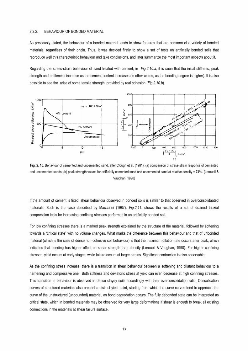
Regarding the stress-strain behaviour of sand treated with cement, in Fig.2.10.a, it is seen that the initial stiffness, peak

strength and brittleness increase as the cement content increases (in other words, as the bonding degree is higher). It is also

possible to see the arise of some tensile strength, provided by real cohesion (Fig.2.10.b).

Fig. 2. 10. Behaviour of cemented and uncemented sand, after Clough et al. (1981): (a) comparison of stress-strain response of cemented

and uncemented sands; (b) peak strength values for artificially cemented sand and uncemented sand at relative density = 74%. (Leroueil &

Vaughan, 1990)

If the amount of cement is fixed, shear behaviour observed in bonded soils is similar to that observed in overconsolidaated

materials. Such is the case described by Maccarini (1987). Fig.2.11. shows the results of a set of drained triaxial

compression tests for increasing confining stresses performed in an artificially bonded soil.

For low confining stresses there is a marked peak strength explained by the structure of the material, followed by softening

towards a “critical state” with no volume changes. What marks the difference between this behaviour and that of unbonded

material (which is the case of dense non-cohesive soil behaviour) is that the maximum dilation rate occurs after peak, which

indicates that bonding has higher effect on shear strength than density (Leroueil & Vaughan, 1990). For higher confining

stresses, yield occurs at early stages, while failure occurs at larger strains. Significant contraction is also observable.

As the confining stress increase, there is a transition in shear behaviour between a softening and dilatant behaviour to a

harnening and compressive one. Both stiffness and deviatoric stress at yield can even decrease at high confining stresses.

This transition in behaviour is observed in dense clayey soils accordingly with their overconsolidation ratio. Consolidation

curves of structured materials also present a distinct yield point, starting from which the curve curves tend to approach the

curve of the unstructured (unbounded) material, as bond degradation occurs. The fully debonded state can be interpreted as

critical state, which in bonded materials may be observed for very large deformations if shear is enough to break all existing

connections in the materials at shear failure surface.

14

Fig. 2. 11. Drained triaxial compression tests on artificially bonded soil; e=0.7 [Maccarini (1987) cited by Leroueil & Vaughan (1990)]

In conclusion, the triaxial tests show evidences that: (i) for low confining pressures the transition from a peak strength yield

point to a critical state; (ii) for high confining pressures there is no marked peak strength before reaching the critical state, but

yield is reached at early stage; (iii) it seems to be a relation between the amount of bonding (in this case provided by the

cement) and the peak strength obtained in the tests.

Taking these factors into account, the constitutive model to considerer to correctively describe the behaviour of such

materials has to be an elasto-plastic model, which comprise the pre-yield, yield and post-yield behaviour. They are explained

as follows.

Yield behaviour

Yield is characterized as being a state from which plastic deformations occur and therefore stiffness and strength of the

material change irreversibly. Generally, a yield locus is drawn in a stress space, where three different modes of yielding,

namely, compression, shearing or swelling yield can be defined (Leroueil & Vaughan, 1990). Only yield due to shear and

compression is considered in this work. Fig.2.12 shows a typical (primary) yield locus and the distinction between the three

types of yielding:

­ compression yield, when yield occurs away from the peak shear strength envelope due to increase average

and/or shear stress (it can be observed in oedometric tests).

15

­ shearing yield, when yield occurs immediately before failure (it can be observed in triaxial tests, where the peak is

identified).

­ swelling yield, when yield occurs because soil structure can no longer retain stored strain energy accumulated in

swelling clay minerals commanded by bonds which are broken due to the effect of increment of vertical stresses

and stiffening due to wetting.

Fig. 2. 12. Different types of yielding (Leroueil & Vaughan, 1990)

Pre-yield behaviour

Before this primary yield be achieved, which in soils is at the very small deformations domain, the behaviour of the material

can be considered to be linear elastic. However, though it is stiff, elasticity can only be truly accepted till axial strain up to

510 . For larger strains, there may be a loss of structure due to stress changes or microslips or closing of microcracks, which

makes the behaviour to be non-linear and non-elastic, yet inside the primary yield curve. Therefore, it is important to

remember that an initial yield will occur before primary yield (Leroueil & Vaughan, 1990). Gens & Nova (1993) suggest that

non-linear elastic behaviour can assumed to be valid within the elastic domain in a first approach. For more refined models,

there can also be an initial yield, marking the ending of the linear elastic regime. In that case, that initial yield would be inside

the primary or main yield locus.

Post-yield behaviour

The degradation of bonds starts to take place after yielding. The material does not lose its structure immediately, but rather

progressively as the strain (irreversible and plastic) increase (Leroueil & Vaughan, 1990) and/or the material is subjected to

wetting/drying cycles (Cardoso R. , 2009). This bonding degradation phenomena is one of the main difficulties to simulate in

the definition of constitutive models for bonded materials, for it must be found a law relating someway the loss of structure

with the irreversible deformations and suction changes. Reference is made to the investigation works of Cardoso et al.

(2013).

16

2.2.3. CONSIDERATION OF BONDING IN CONSTITUTIVE MODELS

In several constitutive models for structures bonded soils, the amount of bonding can be taken into account using a single

parameter b, named as bonding parameter. This parameter, together with the intrinsic properties of the unbonded material

and its yield locus, make possible the definition of the yield locus for the bonded materials. As it regards the structural level of

the bonded material, namelly its connections and arrengement in space, the initial bonding parameter (before any

solicitation) is considered to be indepentent from any constitutive model. Fig.213 shows the effect of various degress of

bonding in the (e,p’) and (q,p’) spaces proposed by Gens & Nova (1993) . When the bonding parametr is null it means that

the material is in the fully debonded state.

In the (e, p’) space, as bonding increases, the virgin isotropic consolidation line moves to the right, wich implies that, for a

given value of p’, a bonded material is able to whithstand a loosser struture that it was impossible if it was unbonded. The

difference in these void ratio, Δe, can be a way of characterizing the amount of bond which is also a way to characterize the

existence of soil structure, as it was illustrated previously in Fig.2.9.

Regarding the yield locus in (q,p’), yield locus of the bonded material is defined relating to the unbonded one (curve A in

Fig.2.13), through the bonding parameter, b. As bonding increases, yield curve grows to the outside (curves B and C),

mantaining its shape since the harnening modulus is isotropic. It is visible that, as bonding increase, compressive strength

improves (parameter p’co given by Equation 2.1) and the material also gains some tensile strength (parameter p’t given by

Equation 2.2), even if much lower than the compressive one. These parameteres are defined in effective stresses when

dealing with saturated materials.

Fig. 2. 13. Virgin isotropic consolidation lines (a) and successive yield surfaces (b) for increasing degrees of bonding.

Boundary AA’ and surface A corresponds to the unbonded material (Gens & Nova, 1993)

)1('' bpp cco (2. 1)

ctt bpp '' (2. 2)

Bond degradation

Models for bonded materials are used to reproduce the evolution of their mechanical behaviour when different loading paths

are applied. This is because stiffness and strength decrease with progressive loss of the bonds, as well as the size of the

yield locus. The way chosen to reproduce this evolution is by changing the parameter b in order to account with plastic

strains.

17

Traditionally, elastoplastic models incorporating damage (h) consider a parameter b (bonding parameter) which reproduce

the degree of connections affecting soil structure and being responsible by extra stiffness and strength. Parameter b is larger

than zero and should be larger for the cases when the amount of bonds are present in the material. This parameter is

reducing when the material is loaded, simulating the effects of bond breakage (or damage) caused by increasind cumulative

plastic deformations until a given reference state is reached (Fig.2.14).

In this work a similar meaning is adopted for parameter b in the sense that it reproduces the improvement of the soil due to

the treatment with cement. However, damage is not considered reason why parameter b will be addressed in this work by

initial bonding parameter, b0. This means that the different dosages have in common only the state corresponding to the

untreated soil, which corresponds to case of b=0.

Fig. 2. 14. Reduction of bonding, b, with increasing damage, h (Gens & Nova, 1993)

This new yield locus after damage is experimentally very hard to assess, in particular because the debondig phenomenon

might not occur in the same way for all the specimens tested. In simplified terms, the change of the locus after yielding takes

into account two phenomena that contribute to this change: (i) the conventional unbounded plastic hardening or softening

(enlargement or reduction of the yield curve, respectively); and (ii) the shrinking of the yield curve due to the degradation of

bonds. These factors are considered by two hardening moduli combined together. The decrease of the bonding parameter is

monotonic and is to zero with a measure of damage of the structure, who by its turn can be function of plastic deformations

(both volumetric and deviatoric), among others. Fig.2.14 sets an example of this relation.

Alonso and Gens (1994) proposed the modification of Gens and Nova (1993) model to account with suction effect in the

structure by using the Barcelona Basic Model, BBM, on the intrinsic yield curve. Suction is not considered in the constitutive

models adopted in this thesis. Still, suction is used to explain some of the obtained results.

Chapter 5 uses the results obtained from undrained triaxial tests performed to define the primary yield curve of each soil-

cement mixture (treated material) prepared with a given dosage of cement. The results found in tests performed in samples

of soil without treatment are used to define the fully debonded state. For so, a given initial bonding parameter is defined for

each material. It must be reaffirmed that the bond degradation is not studied at all and for that reason the bonding

parameters of decreasing dosages do not have any relationship whatsoever to the process of bonding degradation of the

treated soil with the highest cement dosage, for instance. There will be adopted two constitutive models, whose explanation

and assumed hypothesis are explored in that chapter.

18

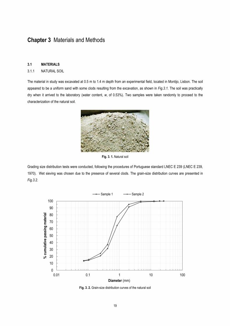
19

Chapter 3 Materials and Methods

3.1 MATERIALS

3.1.1 NATURAL SOIL

The material in study was excavated at 0.5 m to 1.4 m depth from an experimental field, located in Montijo, Lisbon. The soil

appeared to be a uniform sand with some clods resulting from the excavation, as shown in Fig.3.1. The soil was practically

dry when it arrived to the laboratory (water content, w, of 0.53%). Two samples were taken randomly to proceed to the

characterization of the natural soil.

Fig. 3. 1. Natural soil

Grading size distribution tests were conducted, following the procedures of Portuguese standard LNEC E 239 (LNEC E 239,

1970). Wet sieving was chosen due to the presence of several clods. The grain-size distribution curves are presented in

Fig.3.2.

Fig. 3. 2. Grain-size distribution curves of the natural soil

0

10

20

30

40

50

60

70

80

90

100

0.01 0.1 1 10 100

% c

um

ula

tive

pas

sin

g m

ater

ial

Diameter (mm)

Sample 1 Sample 2

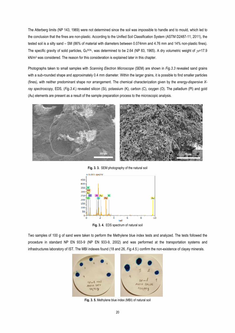
20

The Atterberg limits (NP 143, 1969) were not determined since the soil was impossible to handle and to mould, which led to

the conclusion that the fines are non-plastic. According to the Unified Soil Classification System (ASTM D2487-11, 2011), the

tested soil is a silty sand – SM (86% of material with diameters between 0.074mm and 4.76 mm and 14% non-plastic fines).

The specific gravity of solid particles, GSSOIL, was determined to be 2.64 (NP 83, 1965). A dry volumetric weight of d=17.9

kN/m3 was considered. The reason for this consideration is explained later in this chapter.

Photographs taken to small samples with Scanning Electron Microscope (SEM) are shown in Fig.3.3 revealed sand grains

with a sub-rounded shape and approximately 0.4 mm diameter. Within the larger grains, it is possible to find smaller particles

(fines), with neither predominant shape nor arrangement. The chemical characterization given by the energy-dispersive X-

ray spectroscopy, EDS, (Fig.3.4.) revealed silicon (Si), potassium (K), carbon (C), oxygen (O). The palladium (Pl) and gold

(Au) elements are present as a result of the sample preparation process to the microscopic analysis.

Fig. 3. 3. SEM photography of the natural soil

Fig. 3. 4. EDS spectrum of natural soil

Two samples of 100 g of sand were taken to perform the Methylene blue index tests and analyzed. The tests followed the

procedure in standard NP EN 933-9 (NP EN 933-9, 2002) and was performed at the transportation systems and

infrastructures laboratory of IST. The MBI indexes found (18 and 26, Fig.4.5.) confirm the non-existence of clayey minerals.

Fig. 3. 5. Methylene blue index (MBI) of natural soil

21

3.1.2 GROUT

The grout prepared in laboratory intended to reproduce the grout that would be applied in the execution of the columns made

of Jet Grouting, whereby it was assumed that the materials and its relative proportions to be the same as those used in the

experimental field. Tap water as used since the water in the field was coming from the existing water system. The cement

was a class I Portland cement: CEM I 42,5R (NP EN 197-1, 2012). Its specific gravity of solid particles, GSCEM, is 3.10. As

already said, a water-to-cement ratio of 0.6 in weight was set by the investigation project.

3.1.3 TREATED SOIL (MIXTURE)

The treated soil corresponds to the mixture of the natural soil and the cementitious grout. The mixing process is explained in

Section 3.2.1. The dry volumetric weight of the sand after treatment was assumed to be d=15kN/m3, to account with 15-20%

of solid mass loss during the injection process. For the cement, it was considered a dosage of 150 kg/m3. Table 3.1

summarizes the weights of the three components of the mixture, while Table 3.2 explicit the components ratios in weight.

Table 3. 1. Quantities of materials of treated soil (150kg/m3)

Material Unit Weight (kg/m3)

Cement - CW 150

Water - WW 90

Soil - SW 1500

Table 3. 2. Ratios in weight of the treated soil materials (150kg/m3)

Grout Treated Soil

CW WW SC WW SW WW SCW WW

60.0% 10.0% 6.0% 5.5%

Larger cement dosages were studied by companion authors, namely, 200 kg/m3 (Ribeiro, 2015), 250 kg/m3 and 350 kg/m3

(Oliveira, 2013). The experimental procedures and treatment of the results are similar to the ones regarding the cement

dosage of 150 kg/m3, described in Chapter 4 and Chapter 5, respectively. The results of the laboratory tests of those

dosages will be presented for comparative purposes.

22

3.2 METHODS ADOPTED FOR SPECIMENS PREPARATION

3.2.1 INITIAL REMARKS

Subchapter 3.2 describes the three main stages prior to laboratory testing, specifically: (i) the mixture preparation; (ii) the

preparation of the specimens; and (iii) their curing process and extraction from the moulds for further testing.

As there are some differences in those stages depending on the type of test conducted, an overview of the tests is

synthesized in Table 3.3. Two key analyses were carried out: a macroscopic analysis (macroanalysis) to evaluate the

mechanical and hydraulic properties of the material, and a microscopic one (microanalysis) to perceive changes in its

structure than could explain or agree with the differences observed in the macro tests.

Regarding the macroanalysis, it included unconfined compression tests, Brazilian splitting tests and consolidated undrained

triaxial tests, which are from now on referred as “Mechanical tests” because they give information about strength and

stiffness of the materials and imply the destruction of the samples. The saturated permeability test is called a “Hydraulic test”,

as it gives information about the saturated permeability and it is not destructive. The tests included in the microanalysis were

conducted in independent laboratories, and for this reason they will not be as carefully explained as the other tests.

It is known that the hydro-mechanical properties of the cement evolve with time of cure, with a tendency to stabilize. As it is

usual in current practice when mortar or cement are investigated, the curing times chosen were 3, 7, 14 and 28 days, being

assumed that 28 days are enough for the columns could be used in service. The intermediate days are useful to understand

how and at what pace the properties evolve. The triaxial tests, because they required some time to saturate completely the

specimens and this time would affect the intermediate curing, were only performed for 28 days.

Table 3. 3 Summary of laboratory tests

number of specimens for each curing time

Untreated soil

Treated Soil

3 days 7 days 14 days 28 days

Macroanalysis

Mechanical tests

Unconfined compression test (C) 3

Brazilian splitting test (1) (BR) 4

Consolidated undrained triaxial test (TR) 3 - - -

Hydraulic tests

Saturated permeability test (K) 4(2)

Microanalysis

Scanning Electron Microscope (SEM) 1

Mercury intrusion porosimetries (MIP) 1 - - -

(1) Also known as “splitting tensile strength test”. (2) It is in fact one specimen only, throughout the 28 days. Four readings are taken for each curing time.

23

3.2.3 PREPARATION PROCESS OF THE TREATED SOIL

The treated soil was prepared in the laboratory by mixing the cement, sand and tap water, both manually and mechanically

by using the mixer presented in Fig.3 6.

Fig. 3. 6. Mixer

After sieving the soil through the ASTM sieve #3/8 (diameter of 9.5mm) to separate the larger clods, and weighted the

materials (Fig.3.7. – 1-soil; 2-cement), the water was poured into the mixer container along with two spoons of soil and half

of the amount of the cement (Fig.3.7 – 3). Then, the overall was mixed manually and all of the remaining material was added

(Fig.3.7 – 4; 5). Finally, the mixer was set to work at medium speed (speed 6 out of 10) for 60 seconds and the material

mixed again manually after this period, in order to assure there was no cement deposited in the bottom of the container

(Fig.3.7. – 6 ;7). Finally, the treated soil mixture was ready for specimen preparation (Fig.3.7. – 8).

Fig. 3. 7. Mixture preparation steps

The quantities used for each session of preparation of the mixture, which are enough to prepare four cylindrical specimens to

be used in the mechanical tests, are presented in Table 3. 4. The preparation, by compaction, is explained in Section 3.2.3.

Table 3. 4. Quantities of the mixture for 4 specimens

W cement W water W sand W mix

g g g g

327.59 196.55 3275.86 3800.00

1 2 3 4

5 6 7 8

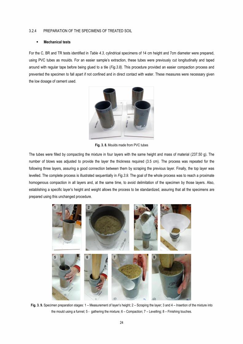
24

3.2.4 PREPARATION OF THE SPECIMENS OF TREATED SOIL

Mechanical tests

For the C, BR and TR tests identified in Table 4.3, cylindrical specimens of 14 cm height and 7cm diameter were prepared,

using PVC tubes as moulds. For an easier sample’s extraction, these tubes were previously cut longitudinally and taped

around with regular tape before being glued to a tile (Fig.3.8). This procedure provided an easier compaction process and

prevented the specimen to fall apart if not confined and in direct contact with water. These measures were necessary given

the low dosage of cement used.

Fig. 3. 8. Moulds made from PVC tubes

The tubes were filled by compacting the mixture in four layers with the same height and mass of material (237.50 g). The

number of blows was adjusted to provide the layer the thickness required (3.5 cm). The process was repeated for the

following three layers, assuring a good connection between them by scraping the previous layer. Finally, the top layer was

levelled. The complete process is illustrated sequentially in Fig.3.9. The goal of the whole process was to reach a proximate

homogenous compaction in all layers and, at the same time, to avoid delimitation of the specimen by those layers. Also,

establishing a specific layer’s height and weight allows the process to be standardized, assuring that all the specimens are

prepared using this unchanged procedure.

Fig. 3. 9. Specimen preparation stages: 1 – Measurement of layer’s height; 2 – Scraping the layer; 3 and 4 – Insertion of the mixture into

the mould using a funnel; 5 - gathering the mixture; 6 – Compaction; 7 – Levelling; 8 – Finishing touches.

1 2 3 4

5 6 7 8

25

Untreated soil specimens

In this work, it was chosen to differentiate the terms “natural soil” and “untreated soil”. The first concerns to the soil

escavated from the experimental field; the latter concerns the same soil with the necessary additional water to prepare the

compacted specimens with a realistic value for the dry volumetric weight in such type of soil. As there was no cement in

these specimens, using the same water content of the treated soil specimens still did not allowed a successful specimen

preparation, whereby more water was added, leading to a water content of 10%. To simulate average field conditions at the

depths where the columns will be built, the dry volumetric weight was considered to be d=17.9 kN/m3. Besides being

realistic, this value is closer to the average dry volumetric weight of all the specimens tested in the scope of this project,

where different dosages of cement were used.

The specimens were prepared in four compaction layers as it was done for the same specimens of treated soil, being the

weight per layer (water and soil) of 247.5 g. Subsequently, the mould was placed inside the oven at 60ºC to dry for 24 hours.

These conditions ensured suction due to capillary effects responsible for the artificial cohesion necessary to perform the

tests. Adding to this, the relatively low temperature applied did not affected the minerals present in the soil.

Table 3.5 presents the main properties of the natural and treated soil with the different cement dosages at preparation. It

worth mentioning that, because the specific gravity of solid particles of the soil and cement are quite different, the

computation of the initial void ratio, ei, of the treated soil has to consider both GSSOIL and GSCEM. This is accomplished

calculating the volume of soil and cement (VS and VC, respectively) contained in a unit volume, VTOT=1m3, as shown in

Equation 3.1. The initial porosity is computed with Equation 3.2.

wCEM

SwSOIL

S

S

wCEM

SwSOIL

S

S

CS

CSTOT

solids

voidsi

G

Wc

G

W

G

Wc

G

Wm

VV

VVV

V

Ve

31

(3.1)

(%)1 i

ii

e

en

(3.2)

Table 3. 5. Main properties of the specimens at preparation

Material d (kN/m3) void ratio, e porosity, n (%) water content, w (%)

Untreated soil 17.9±0.1 0.470 32.0 10.0

Treated soil (150 kg/m3) 16.5±0.1 0.616 38.1 5.5

26

Hydraulic test

For the saturated permeability test, the mixture prepared as described earlier was compacted inside the ring of the

permeameter (2 cm height by 5 cm diameter) in order to have the same dry volumetric weight as that of the cylinders. Two

compaction layers were adopted. This process is illustrated in Fig.3.10.

Fig. 3. 10. Specimen preparation for saturated permeability test

Scanning Electron Microscope, SEM

At the end of the uniaxial compression tests, a small fragment of a tested specimen was collected for SEM photographs

(Fig.3.11). The procedure was repeated for each curing time. After being dried in the oven, the fragment was coated with a

gold/palladium alloy coating at SEM installations (Institute of Materials and Surfaces Science and Engineering, ICEMS, at

IST).

Fig. 3. 11. Example of the collection of the sample for SEM examination

Mercury intrusion porosimetries, MIP

Cubic fragments (1 cm side) were carved from fragments of specimens of untreated and treated soil having 28 days of curing

time, after being tested in unconfined compression tests. They were sent to an external laboratory for MIP analysis

(REQUIMTE at Faculty of Science and Technology of the University Nova de Lisboa).

1 2 3 4

27

3.2.5 CURING AND DEMOULDING

Mechanical tests

After compaction, the specimens were submerged in tap water. They were left in a water container during the curing period

selected for each scheduled test (Fig.3.12). The temperature was approximately constant, ranging from 20ºC to 23ºC.

Fig. 3. 12. Top view of the specimens submerged in a water container

For each curing time, before testing, the samples were weight and the specimens removed from the PVC tube (Fig.3.13).

Then, their weight was measured, as well as their diameter and height. This cylinder was the final geometry of the

specimens for the uniaxial compressive tests and the consolidated undrained triaxial tests. Fig.3.14 shows the two kinds of

specimens after demoulding and before testing: one of untreated soil and one of treated soil.

Fig. 3. 13. Removing the specimen from the mould

Fig. 3. 14. Untreated soil specimen (left); Treated soil specimen (right)

28

For the Brazilian splitting tests (BR), the cylindrical specimens were cut in four disks using a sawing machine in dry

conditions. Each disk had approximately 3.5 cm height. Then, both height and diameter were measured with a calliper rule.

Fig.3.15 (left), illustrates how the identification of the specimen was made: the trial number (next to “BR”) is referred to the

compaction layer that turned into a specimen, the “1” being the upper disc and “4” the lower disk, compacted against the tile.

Fig.3.15 (right) shows the final look of the specimens before the test.

Fig. 3. 15. Identification of the BR specimens (left); Top view of cut specimens (right)

Saturated permeability test

As said, for this test only one specimen was compacted inside the permeameter’s ring. The curing process occurred inside

the permeameter. At the specific end of the intended curing day, four readings were taken, assuming the specimens’ full

saturation. After the last reading, at 28 days of cure, the permeameter was dismantled and the specimen was removed. The

water content then was measured and full saturation was confirmed.

Fig. 3. 16. Specimens inside the permeameter: treated soil at preparation date (left); treated soil after 28 days of cure (centre);

Untreated soil after test (right)

BR 1

BR 2

BR 4

BR 3

29

3.3 EXPERIMENTAL TESTING METHODS

3.3.1 TESTING PLAN

Table 3.6 presents an overview and the terminology adopted for of the laboratory tests followed by the author (dosage of

cement of 150 kg/m3), which are denoted by “curing time (days)” + “test's name abbreviation” + “specimen’s identification”.

The tests performed on untreated soil samples are also included in this table. It was assumed zero days for curing although

there is no cement.

Table 3. 6. Experimental test notation

Untreated soil

Treated Soil (150 kg/m3)

3 days 7 days 14 days 28 days

Macroanalysis

Mechanical tests

Unconfined compression test (C)

0 C1

0 C2

0 C3

3 C1

3 C2

3 C3

7 C1

7 C2

7 C3

14 C1

14 C2

14 C3

28 C1

28 C2

28 C3

Brazilian splitting test (BR)

0 BR1

0 BR2

0 BR3

0 BR4

3 BR1

3 BR2

3 BR3

3 BR4

7 BR1

7 BR2

7 BR3

7 BR4

14 BR1

14 BR2

14 BR3

14 BR4

28 BR1

28 BR2

28 BR3

28 BR4

Consolidated undrained triaxial test (TR)

0 TR1

0 TR2

0 TR3

- - -

28 TR1

28 TR3

28 TR4

Hydraulic test

Saturated permeability test

Micro-analysis

Scanning Electron Microscope (SEM)

Mercury intrusion porosimetries (MIP)

Different dosages of cement are compared later in Chapter 5. In that case, the dosage is made explicit after each label. For

instance, “3 C1 150” stands for the specimen “1” of an unconfined compression test, at 3 days of curing time, made with a

cement dosage of 150 kg/m3.

The next Sections present an overview of each test mentioned in Table 3.6.

30

3.3.2 UNCONFINED COMPRESSION TEST

The unconfined compression tests followed the ASTM standard D2166-06 (ASTM D2166-06, 2006). These tests were

complemented with the measurement of radial displacements, to which local displacement transducers were installed. The

apparatus is presented in Fig.3.17. Loading velocity was 0.2 mm/min, which corresponds to a strain rate of about 0.15%/min,

below the lower limit of the recommended by ASTM standard for soils (0.5%/min). As the strain rate is low, there are no

viscous effects to be considered. Before testing, the initial dimensions of each specimen was measured and annotated.

Fig. 3. 17. Uniaxial compression test apparatus

The outputs of the standard test are (i) given applied load, F; and (ii) change in height of specimen during loading from LVDT

readings, H . Knowing the initial geometrical properties of the specimen (initial average area, A, and height, H0), the axial

compressive stress, a , and the axial strain, a , can be computed using Equations 3.3 and 3.4, respectively:

A

Fa (3.3)

0H

Ha

(3.4)

The correction of the area by Acorr=A/(1-εa) was not considered since only the values of the stress-strain curve until peak

were used and there are some tests showing that it is legitimate to despise the radial deformations until the peak.

Local displacement transducers were used to obtain information regarding radial deformation of the tested specimens and

later to assess the Poisson’s ratio in the elastic domain. This type of transducers were used in IST for the first time and

needed to be calibrated. Their installation process had to be investigated prior to the test, as described as follows.

31

Calibration of the local displacement transducers

When a relative movement occurs between bodies A and B (Fig.3.17.a), there is a variation of the electric potential between

two points which is detected by the transducer. The variation is proportional to the displacement and therefore the

transducers were calibrated by establishing a linear relationship between an imposed displacement, Δd, and the measured

voltage, ΔV. The slope of this linear relationship is called sensitivity. It is valid for displacements applied far from the

transducers’ extremes to avoid non-linear effects between the measured voltages V1 and V2 (Fig.3.18.b and Fig.3.18.c).

a.

b.

c)

Fig. 3. 18. a. Local transducer; b. Device used to apply displacement; c. Calibration of the transducer: [Adapted from (Zensol, 2013)].

The calibration curve is presented in Appendix A.12.The transducers used was an LVDT transducer from GDS and was

installed in an inox ring fixed to cylindrical specimens with 7 cm diameter.

Installation of the transducers

The transducers were placed at the specimen’s mid-height. Firstly, an attempt was made an attempt to fix them to the wall of

the sample using thin metal pins. It was unsuccessful, because the support was not fixed and the ring was moving

progressively with the disaggregation of the sand around the metal pins (Fig.3.19 - left). Then it was decided to support the

ring by using a PVC tube with diameter larger than the specimen’s diameter. It is believed that, by using the PVC tube, no

significant error was introduced since the observed radial deformations during the tests were small, which is explained by the

high stiffness of the treated soil.

32

Fig. 3. 19. Placement of the transducer: first attempt (left) and final placement (right)

Computation of radial deformations

As the transducer and its ring are placed around the specimen, the measured displacement corresponds to the small

increase of the ring’s perimeter thus, it is an increment of arc length, Ld . The increment of diameter Dd is calculated by

Equation 3.5. A schematic drawing of the transducer, ring and specimen when an increase of diameter occurs is presented

in Fig.3.20. Note that the displacement is measured at the mid-line of the ring (Fig.3.20), consequently the radial strain is

calculated for the ring’s initial diameter, Diring, not that of the specimen (Equation 3.6). It is assumed that the deformation of

the ring is identical to the deformation of the specimen.

LDDLD fi

ddd

(3.5) ring

iring

i

rD

L

D

D

dd

(3.6)

Fig. 3. 20. Schematic illustration of the functioning of the transducer placed radially

33

3.3.3 BRAZILIAN SPLITTING TEST

ASTM standard D3967-08 (ASTM D3967-08, 2008) was adopted to perform the Brazilian splitting tests. However, some

changes had to be introduced. The test apparatus is shown in Fig.3.21.a. Different bearing surfaces were used (Fig.3.21.b)

because the tests for each curing time were performed in different occasions, and there was a problem with one of the

surfaces which had to be replaced. This aspect can turn out to be an influence on the result, but it affects mainly the

alignment and centre of the specimens. No bearing strips were used. The loading rate was adequate as the failure happened

within 1 to 10 min of loading. Four specimens with a thickness-to-diameter ratio close to 0.5 were tested for each curing

time. The number of tested specimen was far from the number recommended by the standard (ten), due to schedule

constrains. All mentioned above plus the different boundary conditions may contribute to a larger dispersion of the results as

it will be discussed later in this work.

a. b.

Fig. 3. 21. a. Brazilian splitting test equipment; b. Loading device (top right); Different bearing

surfaces used on natural and treated soil specimens (top right and bottom).

The output of the test is the applied load of failure, Fu. Knowing the average initial geometrical properties of the specimen,

(diameter, D0, and height, H0), the tensile strength, σutensile, of each specimen is computed using Equation 3.7.

00

2

DH

Futensileu

(3.7)

It would be desirable to perform direct uniaxial tensile tests instead of the Brazilian splitting tests since the strength obtained

from the latter test is an indirect value and it is expected to be overestimated. However, in soils, these tests are much simpler

and inexpensive to conduct and the results can be accepted for comparison purposes.

Bearing surface

Loading device Loading device 0 BR

14 BR ; 28 BR 3 BR ; 7 BR

34

3.3.4 CONSOLIDATED UNDRAINED TRIAXIAL TEST

Three compacted specimens for each cement dosage at 28 days of curing time, apart from the untreated soil, were tested

following ASTM standard D4767-11 (ASTM D4767-11, 2011) procedure. One of the chambers used is illustrated in Fig.3. 22.

The specimens’ height-to-average diameter is approximately 2.1, obeying the range from 2.0 to 2.5 pointed by the standard.

The rate strain was approximately 0.07%.

Fig. 3. 22. Consolidated undrained triaxial test apparatus

The saturation was controlled through the measurement of the pore-water pressure parameter (Skempton parameter), B,

computed by Equation 3.6. Theoretically, when B is very close to 1.0, the saturation is considered fully reached. It was

assumed the validity of Skempton’s expression although this is not a traditional material. In fact, due to its cemented

structure its stiffness is much higher than that of an uncemented soil therefore it can be closer to the stiffness of water. This

means that part of the change in the chamber pressure is also bared by the solid skeleton rather than only by the water. The

parameter B never really reached 1.0, but stood close to 0.85. After the tests, the specimens’ water contents were obtained

and the saturation proven to be reached and it was assumed that Skempton Expression would be valid,

sat

satuB

3

, where: (3.8)

satu - Change in the specimen pore-pressure that occur as a result of a change in the chamber pressure when the specimen drainage

valves are closed (saturation phase)

sat3 - Change in chamber pressure (saturation phase)

Regarding the consolidation phase, each one of the three specimens was subjected to a different isotropic consolidation

stresses in order to determine the slope of angle of failure surface. The consolidation stress is isotropic (total and effective) is

the subtraction of the chamber pressure and backpressure at consolidation, ucp. Due to the limitations of the equipment and

the expected strength in cemented soils, fairly small confinement stresses wall applied.

Hydraulic loading device

Triaxial Compression Chamber

Base Plate

Axial Load Piston

Pore-Water Pressure- Measurement Device

Specimen Cap and Base

Rubber membrane

Valves

Top Plate

35

Finally, in the shear phase, the chamber pressure cp was kept constant by closing the water valves, and the axial load, F,

was applied. Table 3.7. presents the expressions used to compute the results shown in Chapter 5, followed by the meaning

of each variable. The end of the test was considered when the axial strain was larger than 10% or the stabilization of deviator

stress, q, and the induced pore-water pressure, Δu.

Table 3. 7. Expressions for treatment of results of the triaxial test

TEST OUTPUT

u Pore-pressure developed during shear

cpu Back-pressure at consolidation stress

cp Chamber pressure

F Given applied Load

H Change in height of specimen during loading from LVDT readings (Axial displacement)

GEOMETRICAL DATA OF SPECIMEN

0H Initial height of specimen

A Initial cross section area of the specimen

Acorr Cross section corrected during shear, by a

corr

AA

1

COMPUTED DATA (shear phase)

a Axial strain for a given applied load 0H

Ha

(3.9)

q Principal stress difference (deviator stress) A

Fq 31 (3.10)

u Induced pore-water pressure at the given axial load cpuuu (3.11)

3 Total minor principal stress / effective consolidation stress cpcp u 3 (3.12)

3' Effective minor principal stress (radial) u 33' (3.13)

1' Effective major principal stress (axial) q 31 '' (3.14)

'p Mean effective stress 3

'2'' 31 p (3.15)

p Mean total stress upp ' (3.16)

The corrections regarding (i) rubber membrane effect; and (ii) height of specimen after consolidation were not calculated

since they were considered insignificant given the material involved (much stronger and stiff than a regular untreated soil).

36

3.3.5 SATURATED PERMEABILITY TEST

The procedure of this test followed the ASTM standard D5084-10 (ASTM D5084-10, 2010). A constant head was applied

using a water pressure controller (Fig.3.23.a-1) and the water was made pass through an interface (Fig.3.23.a-2) and finally

through the permeameter (Fig.3.23.a-3), which is composed by the specimen and two porous stones (top and bottom).

a. b.

Fig. 3. 23. a. Saturated permeability test apparatus (Barata, 2011). b. Details of the permeameter

Once the specimen reaches full saturation and the outlet flow seems to come out at a constant rate, the water is discharged

to four cups, one at a time, in intervals of 15 seconds. This mass of water is then weighted and, through the relationship

given by Equation 3.17, the water flow, Q, is calculated. Knowing the ring geometry, the velocity equals the water flow

divided by the cross-sectional area. The water head is computed by Equation 3.18.

Assuming the validity of the Darcy’s Law, the saturated permeability, kSAT, is determined using Equation 3.19. Table 3.8

summarizes the calculation process described earlier.

Table 3. 8 Expressions for saturated permeability test treatment of results

TEST OUTPUT

m Mass of water measured throughout 15 seconds m = mcup+water - mcup

u Applied water head pressure

GEOMETRICAL DATA OF SPECIMEN

RH Height of the specimen (ring) RD Diameter of the specimen (ring) A Cross section area

FIXED VALUES

15st 3/8.9 mkNw 3/1 cmgw

kPa1u1 00 kPa2u2 00 kPa3u3 00

COMPUTED DATA

Q Water flow [m3/s] wt

mQ

(3.17)

H Water head [m] wuH (3.18)

SATk Saturated permeability [m/s] R

SATHH

AQ

i

vk

(3.19)

Top porous stone

Specimen Water exit

Water entry

37

Chapter 4 Results and Discussion

4.1 INTRODUCTION

This chapter presents the experimental results obtained in each test referred in Chapter 3. The first four subchapters report

the outcomes of the macroanalysis. Initially, an example of the output curves obtained in one test is shown and the

procedures of treatment of results are explained whenever is justified. Then, the results regarding the desired hydro-

mechanical properties are presented and further detailed. This is done for the treated soil specimens prepared with the

cement dosage 150 kg/m3.

Overall results for larger cement dosages studied by companion authors Ribeiro (2015) and Oliveira (2013) are compared

afterwards. These specimens were prepared adopting the same procedures and tests and the treatment of results were

performed as those followed for the cement dosage of 150 kg/m3. The results of tests performed on samples of untreated soil

are also shown, followed by the assessment of the improvement ratio of the treated soil when compared to the untreated

soil.

Lastly, the two final subchapters are referred to the microanalysis. Subchapter 4.6 discusses the combined influence of the

suction and the bonding phenomenon on the results obtained from the macroanalysis. Subchapter 4.7 accounts the results

of MIP and SEM tests, regarding the structure of the treated soil over time, more specifically, of the evolution of size and

distribution of voids (MIP) and visual differences through the analysis of the SEM photographs.

38

4.2 UNCONFINED COMPRESSION TESTS

Uniaxial Compression Tests (C) were performed in three specimens for each curing time and cement dosage. Experimental

setup and the output information to compute are explained on Chapter 3, Section 3.3.2.

4.2.1 EXPERIMENTAL CURVES AND THEIR ANALYSIS

The experimental curves obtained relating both axial compressive stress and radial strain with axial strain, ),( aa and

),( ar , of the “3 C3” specimen are shown in Fig.4.1. The complete set of the results of all the tests is presented in

Appendix A.1, grouped by curing time. Photos of each tested specimen are also displayed there, along with these results, for

later draw conclusions about their failure geometry and the shapes of the curves. .

Fig. 4. 1. “3 C3 150” axial stress-strain and radial strain-axial strain curves

From the curves, the most important information to retain are (i) the unconfined compressive strength, uq ; (ii) the tangent

modulus of elasticity in small strain domain, tgE ; and (iii) the Poisson’s ratio also in small strain domain, . The calculation

of these three parameters is explained next.

0

200

400

600

800

1 000

1 200

0.0E+0 5.0E-3 1.0E-2 1.5E-2 2.0E-2 2.5E-2

σa

(KP

a)

εa

-2.5E-3

-2.0E-3

-1.5E-3

-1.0E-3

-5.0E-4

0.0E+0

5.0E-4

0.0E+0 5.0E-3 1.0E-2 1.5E-2 2.0E-2 2.5E-2

ε r

εa

39

Unconfined compressive strength, uq

Corresponds to the peak value of the axial compressive stress, a , in stress-strain curve ),( aa .

Tangent modulus of elasticity in small strain domain, tgE

The modulus of elasticity in unconfined conditions is generically defined by Equation 4.1, for either secant or tangent moduli.

Its value depends on the axial strain level because the material exhibits non-linear behaviour. Nevertheless, in the linear

elastic domain a single value can be defined. In this work, it was decided to compute a tangent modulus, Etg.

a

a

d

dE

(4.1)

Thus, for each test, the presumed elastic linear domain was isolated and a linear regression adjusted, whose slope

corresponds to Etg. The elastic range chosen for the computation of the linear regression is illustrated in Fig.4.2, for a curing

time of 3 days. Similar figures for the other curing periods can be found in in Appendix A. 4.1. For the definition of the elastic

range, it was admitted that the low values of the stresses for very low strains were not relevant, once they had the influence

of the load cell adjustment and stabilization.

Fig. 4. 2. Linear regression on the elastic range for computation of the modulus of elasticity (curing period of 3 days)

Poisson’s ratio in small strain domain,

The theoretical expression of the Poisson’s ratio is given by Equation 4.2. The computing process was similar to the one

described previously, by linear regression of εr and εa, being the elastic range the same where tgE was computed.

a

r

d

d

(4.2)

E (3 C1 150) y = 82854x - 126.49

R² = 0.9988

E (3 C2 150) y = 149276x - 188.51

R² = 0.9969

E (3 C3 150) y = 89718x - 179.67

R² = 0.9966

0

200

400

600

800

1000

1200

0.0E+00 5.0E-03 1.0E-02 1.5E-02 2.0E-02 2.5E-02

σa

(kP

a)

εa

3 C1

3 C2

3 C3

40

4.2.2 TREATED SOIL - 150 kg/m3

Strength and modulus of elasticity

After the analysis of each stress-strain curve (Appendix A4.1), the first two properties mentioned earlier ( uq and tgE ) were

computed (Table 4.1) and plotted as a function curing time (Fig.4.3 and Fig.4.4, respectively). The red markers in Fig.4.3 and

the bold values in Table 4.1 represent the tests that were not considered for the calculation of the average and standard

deviations values, as well as for the law adjustment rule shown along with the experimental results. The exclusion process of

the tests is explained in Table 4.2.

Table 4. 1. Unconfined compressive test results assessed from stress strain curve

Table 4. 2. Tests’ exclusion process

3 days The three curves are close both in uq and tgE . All the tests were considered.

7 days

The 7 C1 specimen reveals a small plateau at the middle of the curve. The additional strength shown after it could be

explained by the specimen’s heterogeneity or eccentricity of the load. The considered strength was the maximum

compression stress.

The 7 C3 specimen is unusually stiffer (Etg almost 3.50 times higher than the average two others) and for this reason 7 C3

test was excluded.

14 days 14 C1 was excluded because its stiffness and strength about 2 times higher than the tgE and uq obtained for the other

specimens tested with the same curing period.

28 days 28 C1 was excluded as it revealed a uq smaller than the average values for uq measured for 14 days of cure.

Specimen t qu averagestandard

deviation

coefficient

of variation Etg average

standard

deviation

coefficient

of variation

150 kg/m3 days MPa MPa MPa % MPa MPa MPa %

3 C1 3 0.767 82.85

3 C2 3 0.878 149.28

3 C3 3 0.960 89.72

7 C1 7 1.090 102.25

7 C2 7 0.745 154.88

7 C3 7 0.936 436.60

14 C1 14 2.385 448.19

14 C2 14 1.321 223.31

14 C3 14 1.413 180.31

28 C1 28 1.120 444.90

28 C2 28 1.522 192.80

28 C3 28 1.642 372.82

34.0

0.92 0.24 26.55 128.56 37.22 28.9

0.87 0.10 11.13 107.3 36.5

15.1

1.58 0.08 5.34 282.8 127.3 45.0

1.37 0.07 4.76 201.8 30.4

41

Fig. 4. 3. Unconfined compressive strength through time

Fig. 4. 4. Tangent modulus of elasticity in small strain domain through time

From the analysis of Fig.4.3 and Fig.4.4 it is possible to conclude that the evolution with time of both stiffness and strength of

the treated soil has proven to be non-linear, increasing with curing time. The increments in stiffness and in strength with

curing time were larger for the early periods than for the latter. Both mechanical parameters had shown the tendency to

stabilize starting after 14 days of cure. The observed dispersion reflect well the difficulty in achieving homogeneity of the

specimens.

0.0

0.5

1.0

1.5

2.0

2.5

3.0

0 7 14 21 28

unco

nfin

ed c

ompr

essi

ve s

tren

gth

, qu(M

Pa)

curing time (days)

C 1

C 2

C 3

0

100

200

300

400

500

0 7 14 21 28

tang

ent m

odul

us o

f ela

stic

ity, E

tg (

MP

a)

curing time (days)

C1

C2

C3

42

Poisson’s ratio

The results obtained are presented in Table 4.3. Except for the specimen 3 C3, the overall results are clearly very small and

their validity is questionable. The curves of ),( ar in Appendix A4.1 show that the radial strains measured were relevant

only for large axial strains, most likely to be out of the elastic domain. This could be explained by the lack of sensitivity of the

local displacement transducer. The value computed for “3 C3” of ν=0.10, is outside of the range of values commonly found

for sand and cement mortar (0.30 and 0.2, respectively).

Table 4. 3. Poisson’s ratio obtained from the analysis of radial strain – axial strain curve.

There are several explanations for the poor quality of these results. The first, already mentioned, maybe the lack of

sensitivity of the LVDT. The real opening of the ring was very small when compared to the possible range of readings of the

transducer. The second is related with the experimental setup using the PVC tube to support the steel ring with the LVDT. In

fact, the cylindrical specimen also exhibits axial deformation while the ring remains fixed, whereby there will be relative

displacements between the specimen and the ring. Consequently, the radial displacements measured will not actually be at

the middle-height of the cylinder during the test, which is the location where maximum displacements are expected.

However, in the elastic range the axial displacements are very small, so, it is believed that the relative displacement would

not affect the results and this was the reason why the PVC tube was adopted to perform the test.

Specimen ν Specimen ν Specimen ν Specimen ν

3 C1 - 7 C1 -1.20E-03 14 C1 1.90E-03 28 C1 -1.90E-03

3 C2 1.40E-03 7 C2 3.30E-03 14 C2 2.00E-03 28 C2 2.60E-03

3 C3 1.00E-01 7 C3 3.00E-05 14 C3 - 28 C3 2.00E-04

43

Failure geometry

Regarding the failure mode of the tested specimens, it is worth to pay attention to their photos to perceive if the process of

the specimen preparation influences the failure geometry. Fig.4.5 shows the specimens tested at 14 days, which look quite

similar to the rest of the photos presented in Appendix A4.1 for other curing periods.

14 C1 14 C2 14 C3

Fig. 4. 5. Photographs of the specimens after testing at 14 days of cure

From the photos, it is clear to see that the compaction layers became more defined as the specimens were loaded. Typically,

the two top layers (1 and 2, see Fig.3.15, left) are involved in the yielding and rupture of the specimens. This typical

geometry was observed even when the specimens were placed upside down (specimens 3 C2, 7 C3, 14 C3 and 28 C3). In

fact, those layers were the last ones to be compacted and the most exposed to water during the curing process, reason why

it is believed that they could be weaker. It is worth to mention that the heterogeneity observed can also be explained by the

difficult compaction conditions, since the water content of the mixture was very low due to the low water-to-cement ratio of

the grout adopted.

The kind of failure, showing tensile cracks, is typically seen on rock mechanics and is due to the heterogeneity of the

material: there are zones stronger than others are, where the stresses tend to concentrate, relieving other zones until tensile

stresses occur. This type of failure has also been observed by other authors in specimens prepared following this

compaction method (Pierce & Blackwell, 2003; Tang et al., 2007; Cai et al., 2006).

44

4.2.3 TREATED SOIL - All dosages

Similar ways of assessment of the mechanical properties were conducted for the specimens of treated soil with the other

cement dosages: 200 kg/m3 (Ribeiro, 2015), 250 and 350 kg/m3 (Oliveira, 2013). The Poisson’s ratio was not computed for

these specimens, taken into account the poor results obtained for the smaller cement dosage.

The highest cement dosage, 350 kg/m3, required the use of another equipment, namely, an hydraulic load device used for

testing in concrete, since the material’s strength was exceeding the load capacity of the equipment used until then (shown in

Section 3.3.2). Therefore, for this dosage, the first equipment was used to follow up the elastic behaviour of the treated soil

and assess the elastic modulus, until the axial load reached the load capacity. Then, to measure the compressive strength,

the specimens were moved to the other equipment and re-loaded to failure. It is worth mentioning that this second equipment

only recorded the failure force, not being able to find the stress-strain curve.

In Appendix A4.2, the results obtained are compiled in tables and in figures similar to Table 4.1, Table 4.2 and Appendix

A4.1. The summary of results for the qu and Etg parameters along time are shown in Fig.4.6 and Fig.4.7, respectively. The red

filled markers are also the excluded tests. Schematic trend curves are also plotted to make easier the comprehension of the

figures.

Fig. 4. 6. Unconfined compressive strength through time and by cement dosage (Data from Fig.4.3; Ribeiro (2015) and Oliveira (2013)).

0

2

4

6

8

10

12

14

16

18

20

0 7 14 21 28

com

pre

ssiv

e st

ren

gth

(M

Pa)

curing time (days)

150 kg/m3

200 kg/m3

250 kg/m3

350 kg/m3

350 kg/m3

250 kg/m3

200 kg/m3

150 kg/m3

45

Fig. 4. 7. Tangent modulus of elasticity through time by cement dosage (Data from Fig.4.3; Ribeiro (2015) and Oliveira (2013)).

Discussion

From the analysis of Fig.4.6 and Fig.4.7, it is perceptible that the results found in the tests of the specimens of treated soil

with larger cement dosages have the same trends as those observed in specimens of soil on treated with 150 kg/m3. The

improvement of the mechanical properties is most pronounced with increasing amount of cement than with curing time. The

parameter Etg tends to show a higher dispersion of results when compared to qu. One possible explanation is the method of

assessment of Etg, which depends upon the judgment of the person who defines the elastic range where the regression is

being held. In some cases, different elastic ranges change the results, especially when the amount of data is small (such is

the case of the treated soil with the largest dosage). Fig.4.8 illustrates a set of stress-strains for different cement dosages

where it noticeable the increase of both strength and stiffness, besides the fact that the elastic range of axial strain is not the

same for all the tests. The dotted line is a possible continuation of the stress-strain curve drawn, knowing the strength value

and the brittle behaviour expected from the material. The trend of the unconfined compressive stress with increasing time

follows the same pattern of the curves in Fig.2.4, in Chapter 2, and with increasing cement dosage in Fig.2.5. The values

obtained however are practically always above those of the figures. One possible explanation may be because there are

designing charts.

Fig. 4. 8. Stress-strain curves of treated soil at 28 days of curing time for the four cement dosages studied.

0

500

1000

1500

2000

2500

3000

0 7 14 21 28

Etg

MP

a)

curing time (days)

150 kg/m3

200 kg/m3

250 kg/m3

350 kg/m3

0

2

4

6

8

10

12

14

0.0E+00 5.0E-03 1.0E-02 1.5E-02 2.0E-02

qu a

t 28

day

s o

f cu

re (

MP

a)

εa

(possible curve)

350 kg/m3

250 kg/m3

200 kg/m3

150 kg/m3

150 kg/m3

200 kg/m3

350 kg/m3

250 kg/m3

46

4.2.4 UNTREATED SOIL

As explained in Chapter 4, for the test to be possible to be carried out with natural soil, after the samples being prepared with

high water content to make possible the compaction process, the samples were dried 24 h in an oven at 60ºC. This

temperature was low enough to keep the soil minerals unaltered and allowed to install the suction required to provide

strength (cohesion) to the soil. This cohesion assured the specimens not to fall apart before the test.

Similar procedures were followed in the testes performed on the three of untreated soil samples were submitted to the similar

procedures of testing, assuming in a very simplified way that the modulus of elasticity measured was also elastic. The tests

were performed without the local displacement transducer. The stress-strain curves are presented in Fig.4.9.

Fig. 4. 9. Unconfined compression test on natural soil: stress-strain curves

The “0 C2” test differs greatly from the other two tests, mainly in the values of the unconfined compressive strength. This

could be due to either to adjustment problems of the load device or to a much lower suction in that specimen when

compared to the others. Thus, the strength of “0 C2” was not considered to the computation of the natural soil average

strength (bold in Table 4.4.) Also, the elastic range of the curves measured in soil specimens is less defined than those

measured in the tests of the treated soil. Table 4.4 presents the overall results obtained. The photos of the specimens at

failure are shown in Fig.4.10.

Table 4. 4. Unconfined compressive test results assessed from stress strain curve of untreated soil

It is clear the difference of the specimens subjected to drying. Also, the coloration of the top layers is lighter, suggesting a

higher suction installed. The failure geometry is similar to the ones of treated soil specimens. Note that the specimens “0 C2”

E 0 C1 y = 13 055.12x + 42.43

R² = 0.98

E 0 C2 y = 12 034.4397x + 4.0436

R² = 0.9254

E 0 C3 y = 15 099.26x + 3.09

R² = 0.99

0

20

40

60

80

100

120

140

0.0E+00 5.0E-03 1.0E-02 1.5E-02 2.0E-02

σa

(kP

a)

εa

0 C1

0 C2

0 C3

Specimen t qu averagestandard

deviation

coefficient

of variation Etg average

standard

deviation

coefficient

of variation

Nat. Soil days kPa kPa kPa % MPa MPa MPa %

0 C1 0 111.52 13.06

0 C2 0 39.58 12.03

0 C3 0 124.36 15.10

11.65117.94 9.08 7.70 13.40 1.56

47

and “0 C3”, present failure in the 3rd and 4th layers and they were not turned upside down. A possible explanation for this is

the difference of the suction installed. As it is known, the lower the suction, the lower the strength of the material is.

0 C1 0 C2 0 C3

Fig. 4. 10. Failure Photos of untreated soil specimens (Ribeiro, 2015)

Ratios of improvement of the mechanical properties achieved with the treatment adopting different dosages can be

computed considering the average results of the properties of untreated soil in Table 4.4, by dividing each property (average

value) measured for the treated soil by the same property of the untreated soil. The values were computed for both qu and

Etg and are presented in Fig.4.11 and Fig.4.12, respectively.

Strength and stiffness increment with curing time already mentioned are noticeable, as well as the great difference of the

treated soil with 350 kg/m3 of cement and 150 kg/m3. Note that the ratios have more purpose for a comparative analysis. The

actual values are referred to an artificial material, whose water content is much lower than the ones of the treated soil,

meaning that the real improvement ratio could be higher than those presented in this work.

Fig. 4. 11. Improvement ratios of unconfined compressive strength through time and cement dosage

0

20

40

60

80

100

120

140

160

3 7 14 28

impr

ovem

ent r

atio

of q

u

curing time (days)

150

200

250

350

48

Fig. 4. 12. Improvement ratios of elastic tangent modulus of elasticity through time and cement dosage

Regardless of the mechanical parameter or curing time, the increment ratios shows that the amount of cement dosage in soil

is decisive for its behaviour, which indicates that the heterogeneity of the mixture may affect in significant manner the value

of the parameter to be adopted for the column.

Failure figures are similar for all dosages studied, as shown in the photograph presented in Fig.4.13. A specimen prepared

with the cement dosage of 750 kg/m3 was also included to show the contrast between the soil and the soil treated with

increasing dosages and an almost mortar specimen.

Untreated soil 150 kg/m3 200 kg/m3 250 kg/m3 350 kg/m3 750 kg/m3

Fig. 4. 13. Failure photos of tested specimens

0

20

40

60

80

100

120

140

160

3 7 14 28

impr

ovem

ent r

atio

of E

tg

curing time (days)

150

200

250

350

49

4.3 BRAZILIAN SPLITTING TEST

Brazilian splitting tests (BR) were performed in four disk-shaped specimens of each curing time and cement dosage. The

experimental setup and the output information to compute tensile strength are explained on Chapter 3, Section 3.3.3.

4.3.1 TREATED SOIL - 150 kg/m3

Splitting tensile strengths found for each curing time (Equation 3.5, Section 3.3.3), are presented in Table 4.5 and Fig.4.14.

The average height of the disks, H0, is also presented in Table 4.5. All the failure photos are presented in Appendix A.3.

Bold values in Table 4.5 represent the values that were not considered in the calculation of the average and standard

deviations values, and the red filled markers represent the tests that were not considered for further analysis. The criteria for

adopted to choose the invalid tests were: (i) clear deviation from the average values for each curing time or from the

increasing trend of strength over time; (ii) failure geometry far from the diametric line, as exemplified in Fig.4.15.

Fig. 4. 14. Variation of the tensile strength with curing time for 150 kg/m3

Fig. 4. 15. Example of selection of successful tests for 14 days. (left to right: 14 BR 1, 14 BR 2, 14 BR3 and 14 BR 4)

Through the analysis of Fig.4.14, it is possible to conclude that the evolution in time of the tensile strength of the treated soil

is also non-linear. As observed for the unconfined compression tests, the increment with curing time was larger for the early

periods and shows the tendency to stabilize after 14 days of cure.

0

50

100

150

200

250

300

350

0 7 14 21 28

ten

sile

str

eng

th (

kPa)

curing time (days)

BR 1

BR 2

BR 3

BR 4

50

Table 4. 5. Splitting tensile strength (150 kg/m3)

4.3.2 TREATED SOIL - All dosages

Tensile strength was also computed for the specimens of treated soil with the other cement dosages. The results are shown

in Fig.4.16. Appendix A4.4 details the values of the strengths, in tables similar to Table 4.5.

Fig. 4. 16 Splitting tensile strength through time and by cement dosage (Data from Fig.4.14; Ribeiro (2015) and Oliveira (2013)).

Specimen t H0 σutensile average

standard

deviation

coefficient of

variation

days mm MPa MPa MPa %

3 BR 1 3 34.13 0.084

3 BR 2 3 34.55 0.132

3 BR 3 3 35.43 0.133

3 BR 4 3 31.90 0.142

7 BR 1 7 32.15 0.047

7 BR 2 7 34.65 0.113

7 BR 3 7 35.83 0.121

7 BR 4 7 34.05 0.171

14 BR 1 14 36.95 0.307

14 BR 2 14 30.95 0.226

14 BR 3 14 35.25 0.229

14 BR 4 14 33.35 0.270

28 BR 1 28 34.48 0.269

28 BR 2 28 31.80 0.271

28 BR 3 28 30.75 0.282

28 BR 4 28 37.53 0.207

0.136 0.006 4.2

0.146 0.036 24.3

0.227 0.002 0.9

0.276 0.007 2.7

0.0

0.5

1.0

1.5

2.0

2.5

3.0

0 7 14 21 28

ten

sile

str

eng

th (

MP

a)

curing time (days)

150 kg/m3

200 kg/m3

250 kg/m3

350 kg/m3200 kg/m

3

150 kg/m3

250 kg/m3

350 kg/m3

51

Discussion

The general increasing trend of the tensile strength with time and cement dosage is similar to those obtained for the

compressive strength and modulus of elasticity. It is also noticeable a considerable dispersion of results, which tends to

increase with the amount of cement used.

Possible reasons leading to this dispersion are: (i) the difficulty to keep the specimen centred, as it had the tendency to slip

and roll when loaded; and (ii) differences in the specimens’ water content.

In fact, to correctly compare the strengths and adjust trend lines, the dry unit weight and water content of each specimen

ought to be the same. These demands, specially the water content, were hard to be fulfilled in practice, for several reasons.

Right after demoulding it is possible to see, by the colour of the layers, that the degree of saturation is not identical through

the layers. Adding to this, the handling and waiting time between cutting the disks and perform the test, as well as the

changes of relative humidity and temperature of the laboratory, affect the water content of the specimen when is about to be

tested. The water content is related with suction through the retention curve and it is well known that suction significantly

affects the mechanical properties of the soil with or without treatment. This subject is taken up and developed in Section 4.6.

Given this, it would have been desirable to perform a higher number of tests to enhance the statistical significance and have

more confidence in the results.

4.3.3 UNTREATED SOIL

The same tests were conducted in specimens of untreated soil. Fig.4.17. shows the disks after the tests. Clearly, their look is

different from that of the treated soil by either texture or colour. Note that even the “0 BR1” specimen’s colour is much lighter,

because of the drying process.

Table 4.6 presents the values obtained for the four tested specimens. The rupture line is close enough to a diametric line,

apart from the “0 BR1” specimen, which is obviously excluded. Due to its lighter shade, it was believed a greater suction to

be installed, which would lead to a higher tensile strength, but as seen, the figure of failure dictated the much lower value

observed.

Table 4. 6. Splitting tensile strength of the untreated soil specimens

Specimen t σutensile average

standard

deviation

coefficient

of variation

Untreated Soil days MPa MPa MPa %

0 BR 1 0 0.063

0 BR 2 0 0.013

0 BR 3 0 0.016

0 BR 4 0 0.013

0.014 0.002 13.9

52

0 BR 1 0 BR 2 0 BR 3 0 BR 4

Fig. 4. 17 Look of the dried specimen (left); Failure figures of the tested specimens (right)

The improvement ratios of the average tensile strengths for each cement dosage were calculated adopting the same

procedures as when compressive strength and stiffness were analysed considering all the dosages studied. The results are

shown in Fig.4.18. Despite all the experimental imprecisions mentioned earlier, the general trends match to the expectations:

it is noticeable a great improvement of the value of the strength relatively to that of the soil and the increment is larger in

early curing days. The cement dosage is the key factor on the tensile strength because it is directly associated with the

presence of artificial connections of the grains.

Fig. 4. 18. Improvement ratios of tensile strength through time and cement dosage

0

20

40

60

80

100

120

140

160

180

3 7 14 28

impr

ovem

ent r

atio

of

ten

sile

str

enh

gth

curing time (days)

150

200

250

350

53

4.4 CONSOLIDATED UNDRAINED TRIAXIAL TEST

Consolidated Undrained Triaxial tests (TR) were performed in three specimens of untreated and treated soil at 28 days of

curing time. The cement dosages studied were 150 kg/m3, 200 kg/m3 and 250 kg/m3 (Ribeiro, 2015) due to equipment

restrictions. Experimental setup and the output information to compute are explained on Chapter 3, Section 3.3.4.

4.4.1 EXPERIMENTAL CURVES AND THEIR ANALYSIS

The curves of deviatoric stress vs axial strain, ),( aq , and pore-pressure vs axial strain, ),( au , of the specimen “28 TR 3

150” are shown in Fig.4.19. The results of the other two tests are presented in Appendix A4.5. The specimens were

consolidated for 87 kPa, 147 kPa and 235 kPa. They are relatively small stresses because of the equipment maximum

vertical load allowed.

0H 142.0 mm

A 3.74E+3 mm2

cpu 204 kPa

3 235 kPa

Fig. 4. 19. “28 TR 3 150” plots: ),( aq and ),( au (left) ; photo after failure (right)

In each test, two different states are identified, namely:

­ Peak state. In this study the peak state is defined when the ratio q/p’ reaches its maximum value, which

corresponds to the greatest slope of a line (starting from zero) tangent to the effective stress paths of each test

)',( pq . Small deformations are associated with this state, typically around 1%. The slope of the envelope of the

0

500

1 000

1 500

2 000

2 500

3 000

3 500

0 0.02 0.04 0.06 0.08 0.1

q (

KP

a)

dεa

-150

-100

-50

0

50

100

150

0 0.02 0.04 0.06 0.08 0.1Δu

(kP

a)

εa

54

Mohr circles correspondent to peak states and respective angle (peak friction angle), P' , can be computed, as well

as the cohesion, c’P. This cohesion is real due to the presence of bonds provided by the grout.

­ Critical state. Critical state is reached when deviatoric stress, q, and the excess of pore pressure, Δu, stabilize.

The observed critical states occurred for axial strains close to 5%. This value is not as large as it is usually found

for soils, which is larger than 15%. According to theory of Critical States, when the critical state is achieved, the

structure of the material is destroyed, leading to a null apparent cohesion, therefore c’=0. The critical friction angle,

c' , is an intrinsic property of the material. As it will be seen later, the critical state is not reached by any of the

treated materials. This occurs most likely because the bonds were not completely broken. For this reason, for the

treated soil the state where q and Δu stabilize is referred to as “Residual State” from now on in this work and a

residual friction angle R' is computed.

The strength parameters P' , Pc ' and c' or R' were computed for both states, for each specimen. The process of

treatment of results is once again demonstrated for the specimens of treated soil with a cement dosage of 150 kg/m3.

Strength parameters

Through the analyses of the three Mohr circles a friction angle ' and a cohesion, c’, can be obtained for both states

mentioned earlier (Equations 4.6 and 4.7, respectively), by plotting the values of each test in (s’, t), compute a linear

regression y, with slope tan and interception a:

2

''' 31 s (4.3)

2

'' 31 t (4.4)

tanxay (4.5) )arcsin(tan' (4.6)

'cos'

ac (4.7)

Mohr-Coulomb failure criterion:

'tan'' nc (4.8)

Stiffness parameter

The process of computation of the undrained tangent modulus of elasticity in small-strain domain, Eu, is similar to the one

followed in the uniaxial compressive test. The Poisson’s ratio is 0.5 because the test is undrained (Equation 4.9), leading to a

deviatoric strain equal to the axial strain (Equation 4.11). The computation of Eu is given by Equation 4.10:

Undrained test

arrav 2

1020

(4.9)

au

u

s qE

GE

qG

d

d

3

d3

d

(4.10) Deviatoric strain

araras )2

1(

3

2)(

3

2

(4.11)

55

4.4.2 TREATED SOIL - 150 kg/m3

The parameters obtained from the analysis explained in the previous section are shown next, for both peak and critical states

when the distinction is needed.

Strength parameters

PEAK STATES

Table 4.7 presents the set variables that defined the several peak states, from which the Mohr circles in Fig.4.20 were

drawn. Note that the ratios 'pq are very similar, leading to an almost perfect linear regression in ),'( ts .

The strength parameters obtained were a P' of 60.7º and a c’P of 8.3 kPa.

Table 4. 7. Peak state variables

TEST 3 a q u 3' 1' 'pq t 's

kPa - kPa kPa kPa kPa - kPa kPa

28 TR 1 89.0 1.48E-02 472 59 30.0 501.9 2.52 235.93 265.93

28 TR 2 146.3 1.10E-02 1124 69 77.3 1201.3 2.49 562.00 639.30

28 TR 3 237.1 1.07E-02 2758 40 197.1 2955.5 2.47 1379.22 1576.32

Fig. 4. 20. Peak State: effective Mohr’s circles. Peak state envelopes: ( ) in )',( n ; ( ) in )',( st

t = 0.87s' + 4.07 R2=1.00

τ = 1.78 σ'n + 8.32

-2000

-1500

-1000

-500

0

500

1000

1500

2000

0 500 1000 1500 2000 2500 3000 3500

shea

r st

ress

, τ

and

t (k

Pa)

normal effective stress, σ'n and s' (kPa)

28 TR 1

28 TR 2

28 TR 3

56

RESIDUAL STATE

Table 4.8 also presents the values from which the Mohr circles in Fig.4.21 were drawn, this time corresponding to the

residual state. As mentioned before, it can be assumed that this state was reached because both q and Δu became

constant, although the axial deformation was lower than 15%. The marked peak observed in all tests, as well as the

formation of a clear shear surface (Fig.4.23) contribute to this assumption. From the linear regression in ),'( ts the value of

R' =42.2º is obtained.

Table 4. 8. Residual State variables

TEST 3 a q u 3' 1' 'pq t 's

kPa - kPa kPa kPa kPa - kPa kPa

28 TR 1 87.4 1.02E-01 396 -106 192.8 589.0 1.22 198.10 390.90

28 TR 2 147.0 3.74E-02 682 -80 228.1 909.9 1.50 340.91 569.01

28 TR 3 235.0 9.00E-02 1759 -135 372.0 2130.5 1.84 879.27 1251.27

Fig. 4. 21. Residual State: effective Mohr’s circles. Residual state envelopes: ( ) in )',( n ; ( ) in )',( st

Finally, the effective stress paths (p’, q) of the three tests were drawn in Fig.4.22 was well as the envelope of peak states

and the residual state.

t = 0.67 s' R² = 0.97

τ = 0.91 σ'n

-1500

-1000

-500

0

500

1000

1500

0 500 1000 1500 2000 2500

shea

r st

ress

, τ

and

t (k

Pa)

normal effective stress, σ'n and s' (kPa)

28 TR 1

28 TR 2

28 TR 3

57

Fig. 4. 22. Effective stress paths. Mohr-Coulomb envelope in peak and residual states.

It is worth to note that the effective stress paths obtained are never vertical, as they were expected to be in undrained tests.

One possible explanation may be the fact that the specimens were not fully saturated. However, the saturation degree of the

specimens tested were 89%, 92% and 95% for 28 TR 1, 28 TR2 and 28 TR3, respectively. From these values, it is

reasonable to say that the samples were saturated when shear was applied.

Another possibility may be the progressive loss of structure or rupture of the artificial connections between the grains, which

is affecting the overall stiffness of the soil. Another alternative may be the stiffness of the solid skeleton of the treated

material, which may not be reflected when compared to water. This subject was already discussed in Section 3.3.4,

regarding the Skempton parameter.

q = 1.73 p'

q = 2.46 p' + 11.47

0

500

1000

1500

2000

2500

3000

3500

0 200 400 600 800 1000 1200 1400

q (

kPa)

p' (kPa)

28 TR 1

28 TR 3

28 TR 2

ResidualStatesEnvelope

Peak StatesEnvelope

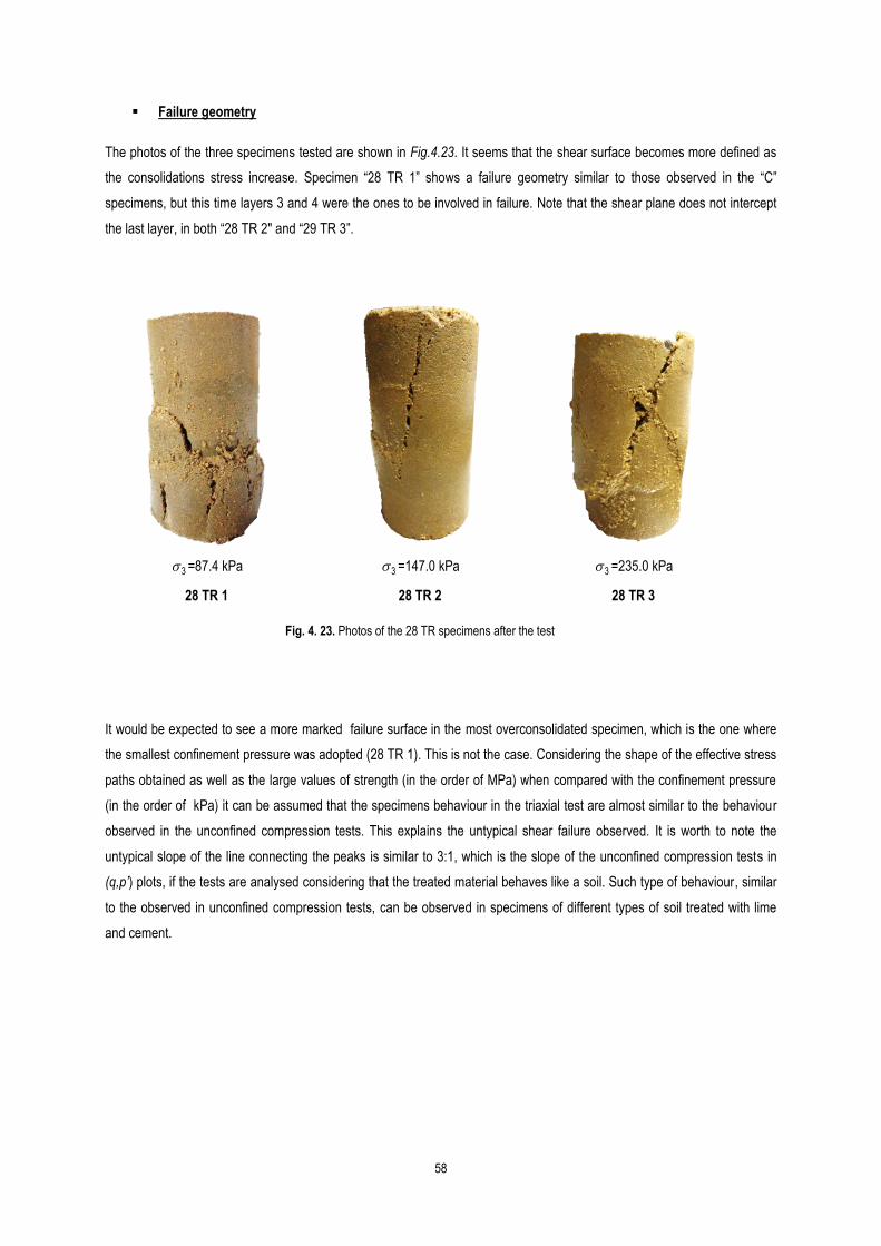
58

Failure geometry

The photos of the three specimens tested are shown in Fig.4.23. It seems that the shear surface becomes more defined as

the consolidations stress increase. Specimen “28 TR 1” shows a failure geometry similar to those observed in the “C”

specimens, but this time layers 3 and 4 were the ones to be involved in failure. Note that the shear plane does not intercept

the last layer, in both “28 TR 2" and “29 TR 3”.

3 =87.4 kPa 3 =147.0 kPa 3 =235.0 kPa

28 TR 1 28 TR 2 28 TR 3

Fig. 4. 23. Photos of the 28 TR specimens after the test

It would be expected to see a more marked failure surface in the most overconsolidated specimen, which is the one where

the smallest confinement pressure was adopted (28 TR 1). This is not the case. Considering the shape of the effective stress

paths obtained as well as the large values of strength (in the order of MPa) when compared with the confinement pressure

(in the order of kPa) it can be assumed that the specimens behaviour in the triaxial test are almost similar to the behaviour

observed in the unconfined compression tests. This explains the untypical shear failure observed. It is worth to note the

untypical slope of the line connecting the peaks is similar to 3:1, which is the slope of the unconfined compression tests in

(q,p’) plots, if the tests are analysed considering that the treated material behaves like a soil. Such type of behaviour, similar

to the observed in unconfined compression tests, can be observed in specimens of different types of soil treated with lime

and cement.

59

Stiffness parameter

The values of the undrained tangent modulus of elasticity at 28 of cure, Eu, computed with Equation 4.10 are presented in

Table 4.9, along with the degree of saturation, Sr, of each specimen. The unconfined compression tests are also shown in

this table.

Table 4. 9. Undrained tangent modulus of elasticity at 28 days of cure and degree of saturation (150 kg/m3)

TEST 3 Eu

or Etg

Sr

kPa MPa %

28 TR 1 89.0 46.08 89.5

28 TR 2 146.3 316.97 92.4

28 TR 3 237.1 576.72 95.1

28 C 2 0 192.80 62.5

28 C 3 0 372.82 76.6

The values of Etg and Eu are shown in Fig.4.24. Concerning the Eu values, because the consolidation stress varies from test

to test, they are also different and tend to increase with increasing confinement stress or consolidation stress. Much higher

Etg was measured in the uniaxial compression tests, than in the triaxial tests under low confinement pressure. This can be

explained by the method used for its definition or by the degree of saturation of the specimens when the “C” tests were

performed. In fact, there are being compared two different moduli of elasticity, namely a saturated (Eu) and an unsaturated

one (Etg). Being so, it is natural that the first is higher than the latter, because suction improves the mechanical properties of

the materials.

Fig. 4. 24. Moduli of elasticity of 28 days specimens of C and TR tests, varying with confinement stress (150 kg/m3)

0

100

200

300

400

500

600

700

800

0 50 100 150 200 250

Etg

, Eu (

MP

a)

σ3 (kPa)

TR tests

C tests

60

4.4.3 UNTREATED SOIL and TREATED SOIL – All dosages

Similar analysis ware conducted for the other dosages of cement and untreated soil (Ribeiro, 2015). The Mohr circles and

envelope of the peak states found for 150, 200 and 250 kg/m3 are presented in Fig.4.25. Similarly, Mohr circles of critical and

residual states are shown in Fig.4.26. The overall strength parameters are shown Table 4.10. The experimental curves of the

tests of untreated soil, 200 and 250 kg/m3 are presented in Appendixes A.6, A.7 and A.8, respectively.

Fig. 4. 25. Effective Mohr circles and envelope to Mohr-Coulomb circles of peak states

Fig. 4. 26. Effective Mohr circles and Mohr-Coulomb residual state envelope

-5000

-4000

-3000

-2000

-1000

0

1000

2000

3000

4000

5000

0 2000 4000 6000 8000 10000 τ (

kPa)

σ'n (kPa)

Peak 150

TR 1 150

TR 2 150

TR 3 150

Peak 200

TR 1 200

TR 2 200

TR 3 200

Peak 250

TR 1 250

TR 2 250

TR 3 250

-2000

-1500

-1000

-500

0

500

1000

1500

2000

0 1000 2000 3000 4000 τ (

kPa)

σ'n (kPa)

Peak 150

TR 1 150

TR 2 150

TR 3 150

Peak 200

TR 1 200

TR 2 200

TR 3 200

Peak 250

TR 1 250

TR 2 250

TR 3 250

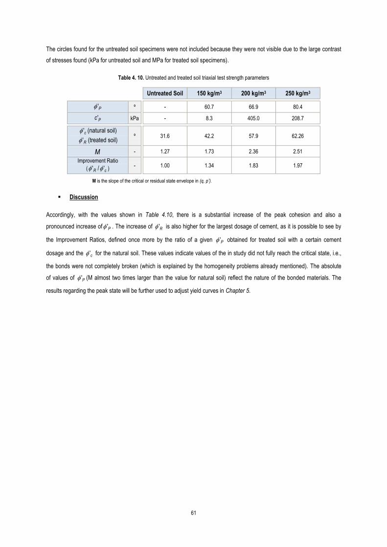
61

The circles found for the untreated soil specimens were not included because they were not visible due to the large contrast

of stresses found (kPa for untreated soil and MPa for treated soil specimens).

Table 4. 10. Untreated and treated soil triaxial test strength parameters

Untreated Soil 150 kg/m3 200 kg/m3 250 kg/m3

P' º

- 60.7 66.9 80.4

Pc ' kPa

- 8.3 405.0 208.7

c' (natural soil)

R' (treated soil) º

31.6 42.2 57.9 62.26

M -

1.27 1.73 2.36 2.51

Improvement Ratio

( R' / c' ) -

1.00 1.34 1.83 1.97

M is the slope of the critical or residual state envelope in (q, p’).

Discussion

Accordingly, with the values shown in Table 4.10, there is a substantial increase of the peak cohesion and also a

pronounced increase of P' . The increase of R' is also higher for the largest dosage of cement, as it is possible to see by

the Improvement Ratios, defined once more by the ratio of a given P' obtained for treated soil with a certain cement

dosage and the c' for the natural soil. These values indicate values of the in study did not fully reach the critical state, i.e.,

the bonds were not completely broken (which is explained by the homogeneity problems already mentioned). The absolute

of values of P' (M almost two times larger than the value for natural soil) reflect the nature of the bonded materials. The

results regarding the peak state will be further used to adjust yield curves in Chapter 5.

62

4.5 SATURATED PERMEABILITY TEST

4.5.1 TREATED SOIL - 150 kg/m3

The saturated permeabilities were computed using Equation 3.19. The values found are plotted in Fig.4.27. The numerical

values are presented in Appendix A.9, and the average values on Table 4.11.

Table 4. 11. Average Saturated permeability values, kSAT (150 kg/m3)

t average standard deviation coefficient of variation

days m/s m/s %

3 2.96E-07 1.01E-07 34.16

7 2.46E-07 1.21E-08 4.91

14 1.22E-08 5.74E-09 47.00

28 8.35E-09 3.00E-09 35.95

Fig. 4. 27. Saturated permeability (150 kg/m3)

As expected, the permeabilities assessed follow a decreasing trend with curing time, being the saturated permeability at 28

days of cure already similar to those found in clays (Kulhawy & Mayne, 1990).

4.5.2 UNTREATED SOIL and TREATED SOIL – 150, 200 and 250 kg/m3

Similar tests were performed on treated soil specimens with 200kg/m3, and 250 kg/m3 of cement (Ribeiro, 2015). The values

found are plotted in Fig.4.28 and the average values in Table 4.12. The numerical values are also presented in Appendix

A.9.The saturated permeability for 200 kg/m3 was only correctly measured for 3 days of cure. As it concerns the untreated

soil, the tests were performed but revealed unreliable, as the equipment was not functioning well at the time. However, it is

known that the normal range of permeability for silty sands is 10-5 to 10-7 m/s (Kulhawy & Mayne, 1990). In Fig.4.28, the

plotted value for the silty sand (untreated soil) was of 10-6 m/s.

1E-09

1E-08

1E-07

1E-06

0 7 14 21 28

k SA

T (

m/s

)

curing time (days)

63

Table 4. 12. Average Saturated permeability values, kSAT (200 and 250 kg/m3)

Fig. 4. 28. Saturated permeability of untreated and treated soil

Discussion

The overall decreasing trends meet the expectations regarding both their evolution with curing time and cement dosage. The

soil treated with 250 kg/m3 at 28 days of cure is less than two orders of magnitude than the silty sand, which confirms the

drastic reduction of permeability that justifies Jet Grouting technique to be used for groundwater control.

t average standard deviation coefficient of variation

days m/s m/s %

3 5.82E-08 1.32E-08 22.73

7 - - -

14 - - -

28 - - -

3 6.86E-09 1.96E-09 28.53

7 6.03E-09 2.13E-09 35.38

14 3.38E-09 9.74E-10 28.81

28 1.91E-09 5.88E-10 30.82

200

kg/m

325

0 kg

/m3

1E-09

1E-08

1E-07

1E-06

0 7 14 21 28

k SA

T(m

/s)

Curing time (days)

Silty Sand

150 kg/m3

200 kg/m3

250 kg/m3

64

4.6 BONDING AND CAPILLARY EFFECTS

The water content of the samples used for the C and BR tests was near to the saturation water content, but not equal. For

this reason, it must be acknowledged that there is a suction installed, even if small. The relationship between suction and

water content is given by the water retention curve (WRC). Fig.4.29 shows a typical WRC, which can be found in clays and

silts. This curve is defined for a given initial void ratio and it presents some hysteresis for drying and wetting paths. For the

case of the treated materials, it is difficult to determine in practice this curve during the curing process, as the water content

is changing during the measurement. After 28 days, it can be assumed that wetting or drying applied to measure this curve

will no longer affect the structure and permeability of the treated material.

Fig. 4. 29. Example of a water retention curve

Considering the compaction procedure adopted to prepare the specimens and the curing process, for intermediate curing

periods it can be assumed that suction is decreasing progressively until the limit case of full saturation. Full saturation is very

hard to be achieved because air bubbles will always be trapped in the voids.

It is known that stiffness and strength increase with increasing suction and decrease with decreasing suction. Accordingly, to

this, it would be expected stiffness and strength to decrease along curing time. However, experimental tests show the

opposite behaviour: the mechanical properties improve with curing time. That means that the suction cannot explain the

mechanical properties observed. As expected, bonding is the controlling agent, as the sand grains are connected by

minerals resultant from the hydration of cement.

The trend curves relating the mechanical properties with curing time, shown in Fig.4.6, Fig.4.7 and Fig.4.16, were

established for mostly decreasing values of suction, and yet, the effect of bonding makes notice as those properties improve

over curing time (Fig.4.29. – continuous line).

If full saturation was achieved at the early stages of cure, or if water content would be stable (Fig.4.30. – dashed line), then

for a given suction, it would be expectable an even higher improvement because suction reduction due to wetting would not

occur nor worsen the improvements due to bonding.

65

Fig. 4. 30. Improvement of the mechanical properties through curing time: decreasing suction (----); constant suction (- - -)

The question lays on how much higher this improvement would be reflecting in the stiffness and strength increment and

neglecting the opposite suction effect. If the increase of water content ( w =w − wSAT), during cure is small, the decrease of

suction, s , will be small as well. Information about w, wSAT and Sr of each “C” specimen before being tested, is shown in

Table 4. 12. The degree of saturation of the same samples is plotted in Fig.4. 30.

Table 4. 13. Water content parameters before testing (150 kg/m3)

w Sr e w

SAT Δw

- % - - %

3 C1 0.16 71.10 0.60 0.22 6%

3 C2 0.16 68.76 0.62 0.23 7%

3 C3 0.16 73.23 0.60 0.22 6%

7 C1 0.16 71.80 0.60 0.22 6%

7 C2 0.16 73.18 0.60 0.22 6%

7 C3 0.15 65.32 0.60 0.22 8%

14 C1 0.16 71.25 0.60 0.22 6%

14 C2 0.16 71.20 0.60 0.22 6%

14 C3 0.16 72.64 0.60 0.22 6%

28 C1 0.18 79.96 0.60 0.22 4%

28 C2 0.14 62.45 0.60 0.22 8%

28 C3 0.17 76.60 0.60 0.22 5%

In fact, w during cure is small (4% to 8%). Hence, the difference in stiffness and strength after being corrected to account

for suction is also expected to be small.

66

Fig. 4. 31. Degrees of saturation of the unconfined compression tests specimens before testing (150 kg/m3)

For tensile strength, it is harder to discard the influence of suction in the results because the conditions of the test were less

controllable, as already mentioned. In addition, the water contents before testing were not measured.

The effect of bonding is most visible when the evolution curves with curing time of strength and stiffness found of the

different cement dosages are compared. As the amount of cement increase, the outcome minerals resulting from the

hydration reactions of the curing are also in larger number, providing more bonds that improve those mechanical properties.

Bonding also affects the WRC and permeability. However, it is expected small Δw for all cases, therefore, the conclusions to

be taken are identical.

Comparing the degree of saturation of the specimens of the “C” tests and of the “TR” tests (Table 4.9), it is possible to

conclude that the saturation of the specimens is difficult, even with water circulating under pressure Sr ranged from 89% to

95%. It would be interesting to assess if the specimens could reach a higher degree of saturation if they were removed from

the PVC tube at 3 days of cure and left to cure in direct contact with water. This could be a possibility since it was already

concluded that the strength after at 3 days of cure is sufficient for the specimen with the smallest dosage not to fall apart.

0

20

40

60

80

100

3 C1 3 C2 3 C3 7 C1 7 C2 7 C3 14 C1 14 C2 14 C3 28 C1 28 C2 28 C3

Deg

ree

of

Sat

ura

tio

n (

%)

67

4.7 MICROANALISYS

4.7.1 SCANNING ELECTRON MICROSCOPE (SEM)

SEM photographs were taken to analyse the presence of bonds in the treated material, which are the minerals from the

hydration of cement. Different samples were removed from fragments of specimens after the UCS tests. Fig.4.32 compares

the aspects of the natural soil and the treated soil, to perceive grains without the coating of the cement’s hydration minerals.

Natural soil Treated soil (150 kg/m3)

Fig. 4. 32. Overview of the natural soil in contrast with the treated soil

The bonds mentioned throughout this work can be observed more closely in Fig.4.33 for 3 and 28 days of cure. It can be

noted the presence of a coat (lighter shade) involving the grains, which justifies the improvements observed at early stages

of cure. The main differences for the two periods observed are in the thickness and texture of these coating layers. Small

crystals and dendrites (“needles”) are observed for 3 days, and they seem to get smaller after 28 days. Their presence is

attributed to water uptake by the cement.

3 days 28 days

Fig. 4. 33. Evolution of the hydration minerals over time (150 kg/m3)

68

Fig.4.34 shows the SEM photographs taken to the specimens of treated soil with the other dosages studied. It can be seen

the same white coating of the grains corresponding to the cement hydration minerals. From the photographs, it is not

possible to get information regarding the amount of minerals because only a small and non-representative part of the

specimen is analysed.

3 days 28 days

150

kg/m

3

200

kg/m

3

250

kg/m

3

350

kg/m

3

Fig. 4. 34. Evolution of the hydration minerals with time and cement dosage

69

4.7.2 MERCURY INTRUSION TESTS (MIP)

Finally, MIP tests were performed to characterize, in approximate manner, the pore-size distribution of the untreated and

treated soil samples for all the cement dosages tested. This information is important to explain mainly the values of kSAT

found. Only the case after 28 days of cure was studied because it is the time from where the soil structure is becoming more

stable and therefore, the waiting period until the tests would not affect their properties. The results are presented in Fig.4.35

and Fig.4.36.

Fig. 4. 35. Porosimetries of natural soil and treated soil with cement dosage of 150 kg/m3.

Comparing the lower dosage of cement with the natural soil, the size of the pores seems to become uniform. Also,

micropores begin to appear, as a result of the presence of the minerals from the hydration of the cement.

Fig. 4. 36. Porosimetries of treated soil with four cement dosages.

0.00

0.05

0.10

0.15

0.20

0.25

0.30

0.35

0.40

1 10 100 1000 10000 100000

Po

re S

ize

Dis

trib

uti

on

Cu

rve

Pore size (nm)

SOIL 150kg/m3

Microporosity Macroporosity

0.00

0.05

0.10

0.15

0.20

0.25

0.30

0.35

0.40

1 10 100 1000 10000 100000

Po

re S

ize

Dis

trib

uti

on

Cu

rve

Pore size (nm)

150kg/m3 200kg/m3 250kg/m3 350kg/m3

Microporosity Macroporosity

70

From the analysis of Fig.4.36, it can be observed a growth of microporosity with the increasing amount of cement, and also a

tendency towards uniform pore sizes with small diameters, as the peaks get less pronounced. This can be explained by the

presence of the hydration minerals of the cement that involve and the grains of silt and sand, as it was observed in the SEM

photographs shown in Fig.5.34. The amount of macropores decrease as the dosage of cement increase, which is due to the

presence of fines of the new minerals (diameter smaller than 75 μm) occupying the large voids between the soil grains.

To conclude, the size of the macropores decreases while the presence of micropores becomes evident. This is in

accordance with the evolution of kSAT because water flowing paths inside soil are mainly through macropores. If their size

decreases, this means that kSAT also decrease, as it is more difficult to water to flow within the soil particles coated with

cement hydration minerals with increasing stiffness.

71

Chapter 5 Consideration of bonding in the adjustment of yield curves

The aim of this chapter is to reproduce the yield curves of the treated materials based on the TR tests results previously

described. Two different elastoplastic models will be adopted for this curve. Later, all the dosages will be related considering

the existence of bonding to reproduce the differences. The untreated soil is considered a reference state. The initial bonding

parameters for each dosage are assessed from the yield curves and later compared to those estimated through the

conventional tests (“C” and “BR”) and further conclusions are taken.

5.1 BASIC CONCEPTS OF YIELD SURFACES

The yield curves to be drawn are defined with two elastoplastic models, namely, the Modified Cam-Clay model and the

model proposed by Nova (1988), referred in (Gens & Nova, 1993) . Fig.5.1 shows the yield space considered in the Original

Cam-Clay model, from which those models are based on, which is defined in terms of isotropic stress, p’, deviatoric stress, q

and specific volume, v. It can be identified (i) the critical state line, CSL; (ii) the normal compression line, NCL; (iii) elastic

compression lines, k-lines; (iv) yield curves;

p'vvlinek k ln:

p'λNv

qNCL

ln

0:

p'λv

Mp'q : CSL

ln

Fig. 5. 1. Original Cam-Clay Model: yield space definition [Adapted from (Maranha das Neves, 2006)]

It is important to distinguish between yield curve (intersection between the elastic wall and yielding surface, which is given by

k-line equation when q=0) and constant volume section, because both are yield curves but correspond to different shapes

when projected in the (q, p’) space. Points of the same yield curve, in both (q,p’) and (v,p’) spaces, belong to different

sections of constant volume, if they were sheared after different consolidation stresses, σ3, taking into account that the

correspondent volumes are different.

72

The theoretical effective stress paths followed in consolidated undrained triaxial test are shown schematically in Fig.5.2. For

a given specific volume, because there is no volume changes, p’ in constant in the elastic domain (until the yield curve is

reached (Fig.5.2 - 3 to 3’), after which p’ increases until reaching the critical state, moving in the constant volume section

(Fig.5.2 – 3’ to 3’’).

The constant volume section are usually asymmetrical with a peak on the dry side, as shown in Fig.5.3 Pd stands for the

peak of the ratio q/p’ (3’), Pq is the peak of q and Fu (3’’) the q of critical state.

Fig. 5. 2. Stress paths of undrained triaxial tests on the dry side

Fig. 5. 3. Asymmetry of the constant volume section (Maranha das Neves, 2006)

The two reference models chosen to define the yield curves for the different cement dosages were the Modified Cam Clay

Model and the model described in Nova (1988) that will from now on be referred as to “MCC” and “Nova”, respectively. The

first for its simplicity, the second for being referred by Gens & Nova (1993) for describing failure on the dry side better than

the classic Cam-Clay model. To compare both models, an associated flow rule was considered for Nova’s model. The yield

functions are given Equations 5.1 and 5.2, respectively.

73

MCC 0'*)''*(2

2

pppM

qf co

(5.1)

Nova 0*)9

2)1(

2

3(/'*ln)3(3 2*

ocppf (5.2)

The parameters necessary for their definition are presented as follows:

c

cM'sin3

'sin6

(5.3)

tppp ''* (5.4)

'*/* pq

(5.5)

rule) (normality 3 (5.6)

23

2

39

2

9

MM

M

(5.7)

The parameters regulating the size of the yield curve are p’co and p’t, given by Equations 5.8 and 5.9, which control the

yielding in isotropic compression and the tensile strength, respectively. With loading or suction changes, the bonding

parameter b decreases after an initial value, b0, due the development of plastic strains. In this work, as mentioned before,

bonding parameter only concerns the initial situation before any bonding damage, and is intrinsically dependent on the

dosage of cement, as is it most likely that more quantity of cement leads to larger formations of hydration minerals.

Since it affects only the size of the elastic domain by affecting p’co and p’t, it can be considered in any constitutive model

adopted. More complex functions relating the bonding with damage and the latter’s dependence on the plastic strains could

be used. Still, there is not an unambiguous way to measure the bonding (Gens & Nova, 1993). The reference curve given by

parameter p’c corresponds to the yield curve of the untreated soil.

)1('' bpp cco (5.8)

ctt bpp '' (5.9)

74

5.2 DATA FROM UNDRAINED TRIAXIAL TESTS

Observed stress paths

The peak states obtained in the TR tests presented in Chapter 4 for all the dosages tested in those conditions were plotted in

(q, p’) (Fig.5.4.a) .They can be aligned with a straight line defined as '92.2 pq . Similar results were found in cement-

admixed Bangkok Clay (Lorenzo & Bergado, 2006) shown in Fig.5.4.b. The same authors name this line by failure envelope.

a) b)

Fig. 5. 4. (a) Stress paths until peak (yield) states and (data of 200kg/m3 and 250kg/m3 from (Ribeiro, 2015));

(b) Stress paths corresponding to p’c of 100 and 200 kPa (Lorenzo & Bergado, 2006)

Fig.5.4 shows a unique regression for all dosages. However if each on would be treated independently from the others it

would be seen that the slope of the “failure envelope” increases with the dosage of cement.

As mentioned in Chapter 4, it is observed that the effective stress paths of the tests do not match the expected vertical path

shown in Fig.5.2 and noted in some paths on Fig.5.4.b. In fact, the stress paths found are very close to what should be

expected in a drained triaxial test, because they are close to the relationship '3 pq . Important pore-water pressures

were measured in the triaxial tests performed because they were done in undrained conditions, as shown in Fig.5.3.b,

therefore the look of the effective stress paths obtained could be explained by other reasons such as the presence of bonds

stiffening the material. This becomes more evident as the dosage of cement increases, supporting this idea. In fact, the

q = 2.92 p' R² = 0.99

q = 1.27p'

0

1 000

2 000

3 000

4 000

5 000

6 000

7 000

8 000

9 000

10 000

0 1 000 2 000 3 000 4 000

q (

kPa)

p' (kPa)

150 kg/m3

200 kg/m3

250 kg/m3

Peak States

TR 1 150

TR 2 150

TR 3 150

TR 1 200

TR 2 200

TR 3 200

TR1 250

TR 2 250

TR 3 250

200

250

Linear (PeakStates)Untreated soilcritical state

75

stiffness of the solid skeleton is not negligible when compared with that of water, which means that the load is distributed

both by the liquid and solid phases.

These results suggest future difficulties in adjusting yield curves of the constitutive models. Note that '0.3 pq is the space

that stands for the unconfined compression tests in soils with no tensile strength therefore the TR tests seem to be very

close to this behaviour/state. This can be accepted if the magnitude of the confinement stresses (pre-shear consolidation

stresses, σ3) applied and that of the shear stresses found are compared. Confinement stress is actually very small, so,

behaviour close to simple compression can be expected.

The output curves of the undrained triaxial tests for the cement dosage of 150 kg/m3 are presented in Fig.5.5. Similar results

for the other dosages can be found in Appendix A.5.1. The behaviour showing marked peak and critical states is coherent to

what is expected from “traditional” soils on the dry side of the yield curve, such as dense sands or overconsolidated clays. In

fact, peaks are observed both in deviatoric stress and in the development of pore-water pressures. However, the amplitude

of the peak should reduce with the increase of confinement stresses and the opposite was observed. This result indicates

the behaviour closer to unconfined compression tests already mentioned. However, the confinement effect is not irrelevant

because both the peak value and the critical state value (assumed to be for the largest deformation reached in the test)

increase with it. Increasing stiffness is also observed.

Fig. 5. 5. Deviatoric stress-strain relationship and excess pore-water pressure development (150 kg/m3)

0

500

1 000

1 500

2 000

2 500

3 000

3 500

0 0.02 0.04 0.06 0.08 0.1 0.12

q (

KP

a)

dεa

28 TR 1

28 TR 2

28 TR 3

σ3= 237 kPa

σ3= 146 kPa

σ3= 89 kPa

-150

-100

-50

0

50

100

150

0 0.02 0.04 0.06 0.08 0.1 0.12

Δu

(K

Pa)

dεa

28 TR 1

28 TR 2

28 TR 3

76

Adjustment of the yield curve

The peak state of the triaxial tests performed in treated soil specimens should belong to the same yield curve defined for

each amount of bonding, depending on the cement dosage (Fig.5.6). As mentioned earlier, each test belongs to different

sections of constant volume.

For each dosage, because the specimens were prepared by a standard compaction process and were subjected to the same

curing conditions and load, it is assumed that the three tests belong to the same yield curve, i.e. have the same pre-

consolidation stress, p’co. Instead of being pre-consolidated for p’co and discharged until the pre-shear consolidation stress,

σ3, each specimen was consolidated to a given σ3. In this case, p’co will be estimated when defining the yield curve

mathematically because it is unknown.

Fig. 5. 6. Expectable adjustment of the yield curve to the three testes of a given cement dosage

The curve shown in Fig.5.6 should have been defined considering the existence of tensile strength given by parameter p’t.

The existence of such strength is in accordance of bonding. It will be seen later that the test fitting can only be achieved if it

assumed p’t=0.

The ideal method to assess the pre-consolidation stress while conducting the consolidation phase of the test (isotropic

loading with drainage allowed) would be to follow and control the deformations as the pressure increases, as it is shown in

Fig.5.7. When a clear change on the curve (v, p’) is perceptible, corresponding to the transition from a swelling line (к-line) to

the Normal Compression Line, the pre-consolidation stress would be reached, after which the specimen would be unloaded

until σ3.

Fig. 5. 7. Exemplification assessing p’co during triaxial test

77

This procedure could not be performed for the studied materials, because of equipment limitations. In fact, the chamber

pressures required were way beyond the capacity of the conventional triaxial chambers, as confirmed later in this work.

Probably, such proceedings should be executed using equipment for rock testing. This reason also justifies the decreasing

pre-shear consolidation stresses for increasing dosages of cement, which are condensed in Table 5.1.

Since these pressures are so low (kPa) and being the magnitude of p’co expected to be of the same order of magnitude of

the strength values measured in unconfined compression tests (MPa), it can be roughly considered that they (σ3) are

practically zero. For this reason, for the definition of the yield curve, it was decided to consider only the triaxial test with the

highest deviatoric stress, i.e., the highest σ3.

Table 5. 1. Consolidation stress before shear

σ3(kPa) 28 TR1 28 TR2 28 TR3

150 kg/m3 89 146 237

200 kg/m3 41 91 159

250 kg/m3 10 23 58

Likewise, it was assumed that the tensile isotropic stress, p’t, was zero due to disparity of magnitudes. If linear regressions

were made for the three tests performed for each dosage, the intercepts would be very low and did not increase

monotonically with the cement dosage, as it is possible to see by the values of c’p in Table 4.10 (Chapter 4).

The “C” and “BR” test were not full saturated, so the yield curve is expected to be larger in the tests than in the TR tests.

Due to the stress path and to the very small confinement stresses applied, it is expected a very large value for p’co (Fig.5.8).

Even in that case, p’t is quite small when compared to the expected p’co, hence, in a saturated state p’t will be even smaller.

This was also a reason to assume 0' tp for the posterior adjustment of a yield curve.

Fig. 5. 8. Saturated and unsaturated yield curves for a given cement dosage.

This is equivalent to say that the tensile strength of the bonds is cancelled with the saturation of the specimen, which the

author acknowledges it is a questionable hypothesis because the cement hydration minerals are present even when the

material is fully saturated. For simplification however, and considering the large values expected for p’co, it was assumed

0' tp .

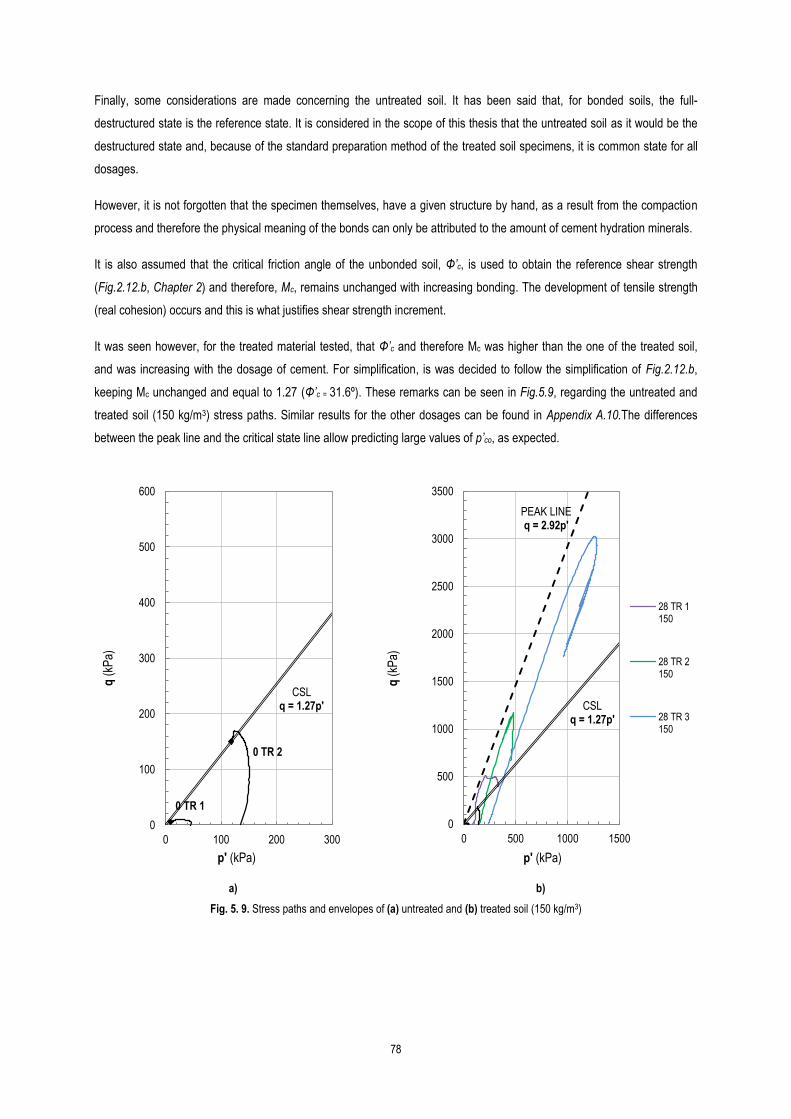
78

Finally, some considerations are made concerning the untreated soil. It has been said that, for bonded soils, the full-

destructured state is the reference state. It is considered in the scope of this thesis that the untreated soil as it would be the

destructured state and, because of the standard preparation method of the treated soil specimens, it is common state for all

dosages.

However, it is not forgotten that the specimen themselves, have a given structure by hand, as a result from the compaction

process and therefore the physical meaning of the bonds can only be attributed to the amount of cement hydration minerals.

It is also assumed that the critical friction angle of the unbonded soil, Φ’c, is used to obtain the reference shear strength

(Fig.2.12.b, Chapter 2) and therefore, Mc, remains unchanged with increasing bonding. The development of tensile strength

(real cohesion) occurs and this is what justifies shear strength increment.

It was seen however, for the treated material tested, that Φ’c and therefore Mc was higher than the one of the treated soil,

and was increasing with the dosage of cement. For simplification, is was decided to follow the simplification of Fig.2.12.b,

keeping Mc unchanged and equal to 1.27 (Φ’c = 31.6º). These remarks can be seen in Fig.5.9, regarding the untreated and

treated soil (150 kg/m3) stress paths. Similar results for the other dosages can be found in Appendix A.10.The differences

between the peak line and the critical state line allow predicting large values of p’co, as expected.

a) b)

Fig. 5. 9. Stress paths and envelopes of (a) untreated and (b) treated soil (150 kg/m3)

CSL q = 1.27p'

0

100

200

300

400

500

600

0 100 200 300

q (

kPa)

p' (kPa)

0 TR 2

PEAK LINE q = 2.92p'

CSL q = 1.27p'

0

500

1000

1500

2000

2500

3000

3500

0 500 1000 1500

q (

kPa)

p' (kPa)

28 TR 1150

28 TR 2150

28 TR 3150

0 TR 1

79

5.3 YIELD CURVES ADJUSTMENT AND BONDING PARAMETER

Yield curves

To define the yield curves of each dosage is necessary to take into account an appropriate constitutive model and an initial

bonding parameter, b0. Being p’c and Mc known because they can be computed using data from the TR tests performed in

the soil specimens, the yield curve of the reference state is perfectly defined. (b0=0).

Fig.5.10 presents possible yield curves obtained for the untreated soil using MCC and Nova models. Only test 0 TR 2 was

considered for its definition. Its effective stress path is presented in Fig.5.9.a, where it can be observed that is almost vertical.

For simplification, and because the soil is slightly overconsolidated so no peak value was found, it was admitted that the

behaviour was elastic the entire stress paths until the CSL was reached. For this reason it was adopted the critical point to

define the yield curve of the untreated soil. Fig.5.11 shows the admitted stress path and yield curve. The values of p’c

obtained are shown in Table 5. 2.

The associated flow rule can also affect the results. However, it was seen that for non-associated flow rules p’c is higher. For

comparative purposes and due to the lack of data, an associated flow rule was adopted and considered acceptable. For a

better definition of this rule, the triaxial tests should have to be performed applying small stress or strain increments after

reaching the peak in order to tackle the evolution of the plastic deformation. From this point further, the p’c to be considered

is 235 or 254 kPa, depending on the constitutive model used. It defines the size of the elastic space in (q, p’) limited by the

yield curve.

Fig. 5. 10. Primary yield curves of untreated soil

0

50

100

150

200

0 50 100 150 200 250 300

q (

kPa)

p' (kPa)

NOVA

MCC

Untreated Soil

80

Fig. 5. 11. Assumption taken for the computation of Mc

Fig.5.12. presents the curves obtained for the soil treated with the different cement dosages, adjusted to the test of highest

(q/p’) ratio, as mentioned earlier. Choosing this criterion means that these curves do not concern the first yielding, but are the

larger possible since that state marks the state from which plastic deformations star to occur. There were some difficulties in

finding solution of f=0 model of Nova for point to the left of the kwon point of the curve. For this reason, the curve until then

was considered to be q=3p’, knowing however in this case the derivate of is not continuous. It is considered that for the

purposes of this work, it is considered that this occurrence has little no influence on further conclusions taken. The pre-

consolidation stresses computed through the adjustment of curves are also presented in Table 5 2.

Table 5. 2. Pre-consolidation stress of untreated soil, p’c, and treated soil, p’co (kPa)

Constitutive model Untreated soil 150 kg/m3 200 kg/m3 250 kg/m3

MCC 237 5357 14 572 20 944

Nova 216 5 300 14 168 19 908

Fig. 5. 12. Yielding curves found for the soil treated with different cement dosages studied: Nova (- - - - -); Modified Cam Clay Model ( )

CSL q = 1.27p'

0

2

4

6

8

10

12

14

0 2 4 6 8 10 12 14 16 18 20 22

q (

MP

a)

p' (MPa)

150 kg/m3

200 kg/m3

250 kg/m3

81

Initial bonding parameter

Knowing the pre-consolidation stresses of the reference (p’c) and bonded yield curves (p’co), it is possible to assess the initial

bonding parameter by using Equation 5.8. Additionally, the ratio p’co/p’c can also be seen as an improvement ratio (Equation

5.10) similarly to the ones described in Chapter 4, Subchapters 4.2.4 and 4.3.3 for the other mechanical tests. Thus, the

initial bonding parameter found for each dosage can be defined as an intrinsic relation of the improvement ratio, IR, by

Equation 5.11.

01'

'b

p

pRI

c

co (5.10)

10 RIb (5. 11)

The initial bonding parameter was evaluated also when the results of the mechanical tests “C” and BR, obtained for all the

treated material at 28 days of curing time, were compared with those obtained for the untreated soil. The improvement ratios,

IR, of the “C” and “BR” tests were defined as being a relationship between the strength of the untreated and treated soil

(Equations 5.12 and 5.13).

soilu

soil treatedutests C

q

qIR

(5. 12)

)(soiltensileu

soil) (treatedtensileutests BRIR

(5. 13)

Equation 5.10 also establishes a relation between stresses, which in this case in particular are yield stresses and not failure

ones, but they limit boundaries of behaviour. By computing b0 as Equation 5.11, the law of bonding is extended to other

cases different from the pre-consolidation yield stress, as Equations 5.14 and 5.15 suggest.

)1( 0bqqsoil

usoil treated

u (5. 14)

)1( 0bsoil tensile

u

soil) (treatedtensileu (5. 15)

The results are presented in Table 5.3 (from Fig.4.11 and Fig.4.14 shown in Chapter 4). The improvement ratios are

summarized accordingly to the cement content of the treated soil samples. The cement content, CC, (Equation 5.12) is

considered instead of the cement dosage to turn the relationship of b0 with the amount of cement independent from the

specific weight of the soil. These values can be compared to those found in the numerical analysis performed to define the

yield curves. The different degrees of saturation of the specimens tested in the different tests are not considered in this

comparison.

SC

C

WW

WCc

(5. 16)

82

Table 5. 3. Comparison between the improvement ratios of the mechanical tests (28 days of cure)

CEMENT DOSAGE

(kg/m3)

CEMENT CONTENT

IMPROVEMENT RATIOS (1+b0) INITIAL BONDING PARAMETER (b0)

C (qu) BR TR (MCC) TR (Nova) C (qu) BR TR (MCC) TR (Nova)

150 0.091 13.4 19.8 22.6 24.5 12.4 18.8 21.6 23.5

200 0.118 40.0 48.9 61.5 65.6 39.0 47.9 60.5 64.6

250 0.143 57.2 56.3 88.4 92.2 56.2 55.3 87.4 91.2

350 0.189 107.3 138.2 106.3 137.2

The comparison of the two types of b0 is shown in Fig.5.13. The dashed line is a regression of the mechanical tests, which

shows that all the parameters are related. It possible to see that the improvement ratios follow very close the trend of those

found in the mechanical tests. The results confirm that the improvement ratios of “C” and “BR” tests can be initially used to

estimate an initial bonding parameter, which by its turn must be a function that increases with the cement content and is

zero for the untreated soil. The simpler function that fulfils these conditions with good adjustment is an potential function,

which equation is included in the same figure.

Fig. 5. 13. Variation of initial bonding parameters differently assessed with cement content

It is worth to note that being the initial bonding defined in such relative terms, it is acceptable to perform other tests, say,

simpler and cheaper ones, in other conditions (for example, non-saturated). This way, an initial bonding parameter can be

estimated, as a first approximation, without needing to perform triaxial test, once the values obtained by modelling follow the

“C” and “BR” fairly closely. The initial bonding parameter can provide important support in the design parameters of a Jet

Grouting Solution.

b0 = 10846CC2.598

R² = 0.8514

0

20

40

60

80

100

120

140

160

0.00 0.05 0.10 0.15 0.20

Init

ial b

on

din

g p

aram

eter

, b0

cement content, CC

C (qu)

BR

TR (MCC)

TR (Nova)

83

5.4 FINAL REMARKS

The calculations of the yielding curves performed are valid if the following assumptions are considered: (i) constant Mc equal

to the value found for the untreated soil; (ii) p’t=0; (iii) isotropic behaviour of the soil, which is reflected in the shape of the

curves; (iv) associated flow rule. Further tests with higher consolidation stresses before shear are necessary to validate

these results. Generally, a larger number of the mechanical tests (“C”, “BR” and “TR”) should be performed in order to better

adjust the curve and find conclusions that are more accurate.

Likewise, more data are necessary to better define the yield curves for the treated material, alternative to those defined by

MCC or Nova. If the aim of this thesis was to define a constitutive model for the treated material, small deformation

increments should be applied near the peak states and specific equipment would be necessary for such analysis, such as on

that would apply different stress paths.

Accordingly, to the definition adopted for b0 this parameter is independent from the constitutive law adopted. Alternative

definitions of b0 could have been adopted. The method used is quite simple, but there other ways to relate certain

characteristic of the material with its initial bonding parameter. McCarter & Desmazes (1997) suggest the relationship

between the electrical resistivity of the material and a cementation factor, m, that can be related somehow with b0, for

example.

The influence of suction was not addressed in this work. However, it is important to remind that suction has also distinct

influence on bonding, especially in it degradation process, as studied by Cardoso (2009). Future steps in the formulation of

the constitutive model would be, for each dosage: (i) to define bonding dependence with suction; (ii) to predict loss of

bonding with loading, related to the cement dosage development of plastic strains and suction change; (iii) to define the pre-

yield behaviour; among others.

84

85

Chapter 6 Conclusions and further investigation

6.1 CONCLUSIONS

A silty sand treated with different dosages of cement was studied in order to characterize its hydro–mechanical behaviour

and assess the improvement in comparison to the untreated material. The grout used in the preparation was fixed by the

research project in which this thesis was developed, having a very low water-to-cement ratio. This restraint led to difficulties

in preparing homogeneous specimens and there are some doubts if the results found reflect the results expected if a more

fluid and realistic grout was used.

The mechanical properties of the treated soil, namely strength (compressive and tensile) and stiffness (modulus of elasticity)

exhibit similar behaviour through the curing time. They all increased along curing time until stable values were reached after

approximately 14 days. The comparison of the results found for the four cement dosages show a far more marked influence

on the improved properties of the treated soil than that of the time of cure. As expected, stiffness and strength increased with

the dosage of cement used independently from curing time.

Some dispersion of results was noted, which suggests that a larger number of tests should be performed and curing

conditions should also have be improved to ensure a more homogeneous a fast saturation of the specimens. Particularly, the

modulus of Elasticity was one of the parameter that showed more dispersion, and it is believed that it was a result of the

adopted assessment method. In fact, by calculating a tangent modulus, the first stages of the test would be forgotten and the

influence of the strain would not be accounted for. The results for the lower dosage show lower dispersion than those found

for greater dosages. This was observed in general for mechanical properties. The local radial displacements transducers

revealed not to the appropriate to measure radial deformations, being impossible to obtain plausible values of the Poisson’s

ratio. It is believed that the sensitivity of the equipment should be higher. In addition, for the Brazilian splitting tests the

conditions should have been more closely controlled, regarding, for example, the bearing surfaces. In this work that was not

possible to ensure since there were some constraints in using the equipment.

Regarding the saturated permeability, the results show a range of permeability with orders of magnitude between the

expected ranges, not being possible to attain a definite relation with curing time and cement dosage for lack of tests and for

not cover all the curing times and cement dosages. Still, the decreasing trend with both curing time and cement dosage meet

to the expectations. In the case where this parameter reveals of being of extreme importance, there should be conducted

more tests using other methods or improve the one used.

At a microscopic level, it is observed that firstly, for 28 days of cure, the pore size decreases as the cement dosage

increases, which is consistent with the filling/involving of the natural soil grains by the cement hydration minerals; secondly,

the SEM photographs also show differences in the amount of hydration minerals and their dimensions. Although the

microscopic test could not be representative (being a “point” in a “universe” of the material), it might be possible to conclude

that changes at the structural level have impact on the revealed behaviour. It is believed that the hydration mineral resulting

from the curing processes are the responsible ones for bonding together the soil particles, providing a stiffer and structure

that is seen and proven by the mechanical tests.

86

Being the treated soil a transition material, challenges in the conduction of the conventional soil tests aroused. The

equipment used for standard soil testing revealed not to be adequate for the triaxial tests performed. Nevertheless, it was

possible to fit the yield curves defined by two elastoplastic constitutive models depending on a given bonding parameter.

Since the initial bonding parameter is defined as the improvement relatively to the unbonded state of the strength properties

of the treated/bonded material, it is verified that conventional tests may be a simple and fast solution to this problem. Or,

alternatively, if only triaxial tests were to be conducted, it is possible to estimate other improved properties of the treated

material if the same properties regarding the untreated soil are known.

The laboratory tests on reconstituted samples aim to reproduce what remains in the ground, reason why so low dosages of

cement were chosen to study. These results could be used to estimate an adequate cement dosage for the soil as long as

there would exist a relationship between the injected volume of grout and its reflux and the actual dosage that remains on the

ground.

Another interesting outcome of the development of this work would be to know by which time it would be possible to start to

load the improved ground after the injection, and time it is affected by the cement dosage. It seems that 14 to 28 days are

enough. Further investigation is needed.

87

6.2 FURTHER INVESTIGATION

The motivating part of this subject would start now: if core and reflux samples were available it would be of interest to

perform the same laboratory tests, compare them and take conclusions about the difference of results between laboratory

and field (if it is more fast and economically viable to perform this kind of test, for instance) and if there is a way of predicting

or estimating the most probable properties to found in the ground, knowing the cement dosage to inject and the estimated

losses. An advantage relatively to the reference values given by literature is that the tests are performed in the actual ground

where Jet Grouting is to be made.

Different preparation methods could be tested in the future. In fact, it could be interesting to find a way of building specimens

that better reproduced the field conditions, or with more homogeneity, knowing by hand that the disruption of the soil due to

the high-pressure injection process is impossible to achieve. The comparison of these results of the ones of this thesis could

also conclude if the preparation method does have a major influence on the results. Also, it would be more correct to ensure

the same initial void index to all the cement dosages.

Adding to this, curing process out could have been done differently. For example, PVC moulds could have been removed

from the samples at 3 days of cure, knowing now that by that time, the material would have been able to maintain its shape

the water have more circulation paths. However, it is worth remembering that even with triaxial chamber pressure the

specimens took time to fully saturate.

Regarding the application of the laboratory test results to the constitutive model, it was made clear that, for a given cement

dosage, though there are noticeable differences between the three test regarding the stiffness and yield strength because of

the different consolidation stress before shear, those stresses are of very little significance when compare to the probable

pre-consolidation stress of the yield curve. Further tests are necessary, in which equipment used to test rock specimens

should be used to ensure enough loading capacity.

More triaxial tests, applying higher chamber pressures, should be done to investigate the best yielding curve to be used in

constitutive modelling. The existence of such model, as well as the knowledge on the relationship between bonding

parameter and cement dosage can be very useful at deigning Jet Grouting solutions.

88

89

References

ASTM D2166-06. (2006). Standard Test Method for Unconfined Compressive Strength of Cohesive Soil. American

Standard for Testing Materials, EUA.

ASTM D2487-11. (2011). Standard Practice for Classification of Soils for Engineering Purposes (Unified Soil

Classification System). American Standard for Testing Materials, EUA.

ASTM D3967-08. (2008). Standard Test Method for Splitting Tensile Strength of Intact Rock Core Specimens.

American Standard for Testing Materials, EUA.

ASTM D4767-11. (2011). Standard test Method for Consolidated Undrained Triaxial Compression Test for Cohesive

Soils. American Standard for Testing Materials, EUA.

ASTM D5084-10. (2010). Standard Test Methods for Measurement of Hydraulic Conductivity of Saturated Porous

Materials Using a Flexible Wall Permeameter. American Standard for Testing Materials, EUA.

Barata, A. R. (2011). Micromechanical explanation for the compressibility of granular materials. Instituto Superior

Técnico, Lisbon (in Portuguese)

Bell, A. (2012). Geotechnical grouting and soil mixing. Chapter 90. ICE Manual of Geotechnical Engineering.

Institution of Civil Engineers, United Kingdom.

Bruce, D. (1994). Jet Grouting. Chapter 8. Ground Control and Improvement. John Wiley & Sons, Inc., New York.

Cai, Y., Shi, B., Charles, W., & Tang, C.-S. (2006). Effect of polypropylene fibre and lime admixture on engineering

properties of clayey soil. Engineering Geology, Volume 87, Issues 3–4, pp. 230-240. ELSEVIER.

Cardoso, Alonso, & Maranha das Neves. (2013). A constitutive model for compacted expansive and bonded marls.

In Géotechnique 63, no.13, pp. 1116-1130.

Cardoso, R. (2009). Hydro-Mechanical Behaviour of Compacted Marls (PhD Thesis), pp. 35-92. Instituto Superior

Técnico, Lisbon

Cardoso, R., & Maranha das Neves, E. (2012). Hydro-mechanical characterization of lime-treated and untreated

marls used in a motorway embankment. Engineering Geology, Volume 133-134, pp. 76-84. ELSEVIER.

Earth Tech – Geotechnical Construction Services. (2013) Jet Grouting. Retrieved September 2013, from:

http://www.earthtech.net/services-and-solutions/down-to-earth-solutions-to-technical-problems/jet-grouting/

Essler, R. & Yoshida, H.(2004). Jet Grouting. Chapter 5. Ground Improvement, Second Edition. Moseley, M. P. and

Kirch, K. Spon Press, London.

90

Gens, A., & Nova, R. (1993). Conceptual bases for a constitutive model for bonded soils and weak rocks. In Symp.

on Geotechnical Engineering of Hard Soils - Soft Rocks, Volume I ,pp. 485-494.

George K. Burke, P. (2010). Archive: Construction. Retrieved September 2013, from Wind Systems:

http://windsystemsmag.com/search/article/?articleID=77

Geosistema. (2013) Jet Grouting. Retrieved September 2013, from:

http://www.geosistema.it/image/image/jet%20grouting/jet2.jpg

Heidelberg Cement. (2013). Applications. Grouting. Retrieved from :

http://www.heidelbergcement.com/NR/rdonlyres/D7C7A8CF-F84B-40D4-9D28-

C04F1D2E7AE1/0/Anwendung_injektionen_jetmix_hdi_duese.jpg

Kulhawy, F., & Mayne, P. (1990). Manual on Estimating Soil Properties for Foundation Design. EL-6800. EPRI, New

York.

Leroueil, S., & Vaughan, P. R. (1990). The general and congruent effects of structure in natural soils and weak rocks.

Géotechnique, Volume 40, no.3, pp. 467-488.

LNEC E 239. (1970). SOIL. Particle-size distribution analysis by wet sieving. National Laboratory for Civil

Engineering, Portugal. (in Portuguese)

Lorenzo, G., & Bergado, D. (2006). Fundamental Characteristics of Cement-Admixed Clay in Deep Mixing. Journal of

Materials in Civil Engineering. SPECIAL ISSUE: Stabilization of Geomedia Using Cementitious Materials,

pp. 161–174.

Lunardi, P. (1997). Ground improvement by means of jet-grouting. Proceedings of the ICE - Ground Improvement,

Volume 1, Issue 2, pp. 65-85. Thomas Telford Services, Ltd, London.

Maranha das Neves, E. (2006). Rock and Soil Mechanics. Instituto Superior Técnico, Lisbon. (in Portuguese)

McCarter, W. J., & Desmazes, P. (1997). Soil characterization using electrical measurements. In Geótechnique,

Volume 47, No. 1, pp. 179-183.

Mitchell, J., & Jardine, F. (2012). A guide to ground treatment. CIRIA, London.

Modoni, G., Croce, P., & Mongiovì, L. (2006). Theorical modelling of jet grouting. Géotechnique, Volume 56, No. 5,

pp. 335-347.

NP 143. (1969). SOILS. Determination of the Atterberg limits. IGPAI, Lisbon. (in Portuguese)

NP 83. (1965). SOILS. Determination of the specific gravity of solid particles. IGPAI, Lisbon. (in Portuguese)

NP EN 197-1. (2012). Cement - Part 1: Composition, specifications and conformity criteria for common cements.

IPQ, Caparica. (in Portuguese)

91

NP EN 933-9. (2002). Tests for geometrical properties of aggregates. Part 9: Assessment of Fines. Methylene blue

test. IPQ, Caparica. (in Portuguese)

Oliveira, H. (2013). Study of the action of grout intended for jet grouting columns in sandy soils. M.Sc. Thesis.

Instituto Superior Técnico, Lisbon. (in Portuguese) (in preparation).

Pierce, C., & Blackwell, M. (2003). Potential of scrap tire rubber as lightweight aggregate in flowable fill. In Waste

Management, Volume 23, Issue 3,pp. 197-208. ELSEVIER.

Pinto, A. (2008). Micropile Foundations and Jet Grouting. Slides from Advanced Formation Diploma in Geotechnics

for Civil Engineering. Instituto Superior Técnico, Lisbon. (in Portuguese)

Ribeiro, D. (2015). Prediction of the hydro-mechanical behaviour of jet-grouting columns made of soil-cement

mixtures”. Ph.D. Thesis. Instituto Superior Técnico, Lisbon (in preparation).

Stroud, M. (1994). Report on Sessions 5 and 6: Jet grouting and soil mixing. Grouting in the Ground. Thomas

Telford, London:

Tang, C., Shi, B., Gao, W., Chen, F., & Cai, Y. (2007). Strength and mechanical behavior of short polypropylene fiber

reinforced and cement stabilized clayey soil. In Geotextiles and Geomembranes, Volume 25, Issue 3, pp.

194-202. ELSEVIER.

Zakladani. (2008). JET GROUTING. Retrieved in September 2013, from Zakládání staveb:

http://www.zakladani.cz/en/jet-grouting

Zensol. (2013). Zensol. Retrieved in July 2013, from: http://www.zensol.com/images/img_motion/fig2_12f.gif

92

93

Appendixes

A.1. Experimental curves and failure geometry of unconfined compressive tests by curing time (150 kg/m3) .......................... 95

A.2. Uniaxial Compression tests: summary of obtained results for treated soil with other cement dosages. ............................ 99

A.3. Pictures of brazilian splitting tests (150 kg/m3) .................................................................................................................. 102

A.4. Splitting tensile strengths (other dosages) ........................................................................................................................ 103

A.5. Output curves of consolidated undrained triaxial tests (150 kg/m3) .................................................................................. 105

A.6. Output curves of consolidated undrained triaxial tests and Mohr-Coulomb circles (Untreated soil) (Ribeiro, 2015) ........ 107

A.7. Output curves of consolidated undrained triaxial tests and Mohr-Coulomb circles (200 kg/m3) (Ribeiro, 2015) .............. 109

A.8. Output curves of consolidated undrained triaxial tests and Mohr-Coulomb circles (250 kg/m3) (Ribeiro, 2015) .............. 113

A.9. Saturated permeabilities (Untreated and tretad soil) ......................................................................................................... 117

A.10. Deviatoric stress-strain curve and excess pore-water pressure development (Ribeiro, 2015) ......................................... 119

A.11. Stress paths off all the tests, until critical state (Ribeiro, 2015) ......................................................................................... 121

A.12. Calibration Curve of the local displacement transducer .................................................................................................... 122

94

95

A.1. Experimental curves and failure geometry of unconfined compressive tests by curing time (150 kg/m3)

3 DAYS

3 C1 3 C2 3 C3

E (3 C1 150) y = 82854x - 126.49

R² = 0.9988

E (3 C2 150) y = 149276x - 188.51

R² = 0.9969

E (3 C3 150) y = 89718x - 179.67

R² = 0.9966

0

200

400

600

800

1000

1200

0.0E+0 5.0E-3 1.0E-2 1.5E-2 2.0E-2 2.5E-2

σ (

kPa)

εa

3 C1

3 C2

3 C3

y = -0.0014x - 9E-06 R² = 0.3667

y = -0.1009x + 0.0003 R² = 0.9835

-2.0E-3

-1.5E-3

-1.0E-3

-5.0E-4

0.0E+0

5.0E-4

0.0E+0 5.0E-3 1.0E-2 1.5E-2 2.0E-2 2.5E-2

ε r

εa

3 C1

3 C2

3 C3

96

7 DAYS

7 C1 7 C2 7 C3

E (7 C1 150) y = 102245x - 825.54

R² = 0.9874

E (7 C2 150) y = 154876x - 601.19

R² = 0.9973

E ( 7 C3 150) y = 436599x - 600.42

R² = 0.9849

0

200

400

600

800

1000

1200

0.0E+0 5.0E-3 1.0E-2 1.5E-2 2.0E-2 2.5E-2

σ (

kPa)

εa

7 C1

7 C2

7 C3

N 7 C1 y = 0.0012x - 7E-06

R² = 0.322

N 7 C2 y = -0.0033x - 1E-05

R² = 0.7354

N 7 C3 y = -3E-05x - 1E-06

R² = 2E-05

-1.0E-3

-8.0E-4

-6.0E-4

-4.0E-4

-2.0E-4

0.0E+0

0.0E+0 5.0E-3 1.0E-2 1.5E-2 2.0E-2 2.5E-2

ε r

εa

7 C1

7 C2

7 C3

97

14 DAYS

14 C1 14 C2 14 C3

E (14 C1 150) y = 448188x - 2169.9

R² = 0.9993

E (14 C2 150) y = 223313x - 431.47

R² = 0.9976

E (14 C3 150) y = 180314x - 1191.2

R² = 0.9985

0

500

1000

1500

2000

2500

3000

0.0E+0 5.0E-3 1.0E-2 1.5E-2 2.0E-2 2.5E-2

σ (

kPa)

εa

14 C1

14 C2

14 C3

N 14 C1 y = -0.0019x + 6E-06

R² = 0.32

N 14 C2 y = -0.002x - 2E-06

R² = 0.6652

-1.0E-4

-8.0E-5

-6.0E-5

-4.0E-5

-2.0E-5

0.0E+0

2.0E-5

4.0E-5

0.0E+0 5.0E-3 1.0E-2 1.5E-2 2.0E-2 2.5E-2

ε r

εa

14 C1

14 C2

14 C3

98

28 DAYS

28 C1 28 C2 28 C3

E (28 C1 150) y = 444901x - 773.63

R² = 0.9929 E (28 C2 150)

y = 192795x - 496.15 R² = 0.9952

E ( 28 C3 150) y = 372823x - 1149

R² = 0.9959

0

400

800

1200

1600

2000

0.0E+0 5.0E-3 1.0E-2 1.5E-2 2.0E-2 2.5E-2

σ (

kPa)

εa

28 C1

28 C2

28 C3

N 28 C1 y = 0.0019x - 3E-06

R² = 0.2054

N 28 C2 y = -0.0026x - 2E-05

R² = 0.6443

N 28 C3 y = -0.0002x - 3E-06

R² = 0.0307

-2.0E-4

-1.5E-4

-1.0E-4

-5.0E-5

0.0E+0

5.0E-5

0.0E+0 5.0E-3 1.0E-2 1.5E-2 2.0E-2 2.5E-2

ε r

εa

28 C1

28 C2

28 C3

99

A.2. Uniaxial Compression tests: summary of obtained results for treated soil with other cement dosages.

Table A4.2. 1. 200 kg/m3 (Ribeiro, 2015)

Note: The values in bold represent the excluded tests.

3 days The three curves are close both in uq and tgE . All the tests were considered.

7 days The 7 C3 specimen is unusually stiffer reason why it was excluded.

14 days 14 C2 was excluded as it revealed a much different curve than the other two.

28 days All the tests were considered.

Specimen t qu averagestandard

deviation

coefficient

of variation Etg average

standard

deviation

coefficient

of variation

200 kg/m3 days MPa MPa MPa % MPa MPa MPa %

3 C1 200 3 3.64 562.40

3 C2 200 3 3.65 731.01

3 C3 200 3 3.51 532.72

7 C1 200 7 4.71 459.62

7 C2 200 7 5.69 804.85

7 C3 200 7 4.42 1407.84

14 C1 200 14 5.08 475.71

14 C2 200 14 2.72 572.37

14 C3 200 14 5.28 947.58

28 C1 200 28 4.39 954.33

28 C2 200 28 5.14 916.67

28 C3 200 28 4.63 1090.51

333.7 46.9

4.72 0.38 8.08 987.2 91.5 9.3

106.9 17.6

5.20 0.70 13.39 632.23 244.11 38.6

3.60 0.08 2.22 608.7

5.18 0.14 2.72 711.6

100

Table A4.2. 2. 250 kg/m3 (Oliveira, 2013)

Note: The values in bold represent the excluded tests.

3 days 3 C2 was excluded because it was unloaded and reloaded close to the failure load.

7 days 7 C1 specimen was unusually stiffer, reason why it was excluded.

14 days 14 C3 after having noted a great deal of instability from the equipment.

28 days All the tests were considered.

Specimen t qu averagestandard

deviation

coefficient

of variation Etg average

standard

deviation

coefficient

of variation

250 kg/m3 days MPa MPa MPa % MPa MPa MPa %

3 C1 250 3 4.31 1106.40

3 C2 250 3 3.52 756.36

3 C3 250 3 4.32 887.27

7 C1 250 7 4.48 2415.85

7 C2 250 7 3.64 940.19

7 C3 250 7 3.16 817.08

14 C1 250 14 6.24 1234.99

14 C2 250 14 4.87 774.14

14 C3 250 14 3.67 524.39

28 C1 250 28 6.63 1867.02

28 C2 250 28 6.71 1676.25

28 C3 250 28 6.90 1546.65

4.31 0.01 0.24 996.8

5.55 0.97 17.52

154.9 15.5

3.40 0.34 9.91 878.64 87.05 9.9

1004.6 325.9 32.4

6.75 0.14 2.11 1696.6 161.2 9.5

101

Table A4.2. 3. 350 kg/m3 (Oliveira, 2013)

Note: The values in bold represent the excluded tests.

3 days All the tests were considered.

7 days All the tests were considered. The strength value of 7 C1 was not considered due to problems with the equipment.

14 days All the tests were considered. The strength value of 14 C1 was not considered due to problems with the equipment.

The stiffness value of 14 C3 was not considered as it was unusually higher.

28 days All the tests were considered. The strength value of 28 C3 was not considered because it isn’t actually a strength,

but a lower limit.

Specimen t qu averagestandard

deviation

coefficient

of variation Etg average

standard

deviation

coefficient

of variation

350 kg/m3 days MPa MPa MPa % MPa MPa MPa %

3 C1 350 3 13.16 1715.88

3 C2 350 3 5.74 1488.89

3 C3 350 3 9.41 1803.88

7 C1 350 7 7.80 1764.84

7 C2 350 7 13.16 1422.17

7 C3 350 7 11.58 1450.37

14 C1 350 14 9.25 1921.09

14 C2 350 14 15.20 1739.04

14 C3 350 14 17.32 2841.67

28 C1 350 28 12.74 2069.83

28 C2 350 28 12.56 2005.37

28 C3 350 28 10.57 1945.66

9.7

12.37 1.12 9.07 1545.79 190.22 12.3

9.44 3.71 39.36 1669.6 162.5

7.0

12.65 0.13 1.03 2007.0 62.1 3.1

16.26 1.50 9.20 1830.1 128.7

102

A.3. Pictures of brazilian splitting tests (150 kg/m3)

3 days

3 BR 1(*) 3 BR 2 3 BR 3 3 BR 4

7 days

7 BR 1(*) 7 BR 2(*) 7 BR 3 7 BR 4

14 days

14 BR 1(*) 14 BR 2 14 BR 3 14 BR 4(*)

28 days

28 BR 1 (*) 28 BR 2 28 BR 3 28 BR 4 (*)

103

A.4. Splitting tensile strengths (other dosages)

A4. 1. 200 kg/m3 (Ribeiro, 2015)

A4. 2. 250 kg/m3 (Oliveira, 2013)

Specimen t σutensile average

standard

deviation

coefficient of

variation

200 kg/m3 days MPa MPa MPa %

3 BR 1 3 0.536

3 BR 2 3 0.534

3 BR 3 3 0.568

3 BR 4 3 0.595

7 BR 1 7 0.339

7 BR 2 7 0.506

7 BR 3 7 0.531

7 BR 4 7 1.188

14 BR 1 14 0.712

14 BR 2 14 0.884

14 BR 3 14 0.758

14 BR 4 14 0.545

28 BR 1 28 0.443

28 BR 2 28 0.585

28 BR 3 28 0.914

28 BR 4 28 0.790

0.558 0.029 5.2

0.519 0.017 3.4

0.785 0.089 11.4

0.683 0.210 30.7

Specimen t σutensile average

standard

deviation

coefficient of

variation

250 kg/m3 days MPa MPa MPa %

3 BR 1 3 0.422

3 BR 2 3 0.497

3 BR 3 3 0.640

3 BR 4 3 0.379

7 BR 1 7 0.732

7 BR 2 7 0.610

7 BR 3 7 0.598

7 BR 4 7 0.868

14 BR 1 14 0.697

14 BR 2 14 0.741

14 BR 3 14 0.725

14 BR 4 14 1.260

28 BR 1 28 1.430

28 BR 2 28 0.742

28 BR 3 28 0.861

28 BR 4 28 0.757

0.433 0.059 13.7

0.702 0.126 17.9

0.721 0.023 3.1

0.786 0.065 8.2

104

A4. 3. 350 kg/m3 (Oliveira, 2013)

A4. 4. Untreated soil

Specimen t σutensile average

standard

deviation

coefficient of

variation

days MPa MPa MPa %

3 BR 1 3 0.781

3 BR 2 3 1.491

3 BR 3 3 1.908

3 BR 4 3 1.630

7 BR 1 7 1.599

7 BR 2 7 1.899

7 BR 3 7 1.989

7 BR 4 7 2.148

14 BR 1 14 1.224

14 BR 2 14 2.458

14 BR 3 14 2.268

14 BR 4 14 1.967

28 BR 1 28 1.510

28 BR 2 28 2.057

28 BR 3 28 1.800

28 BR 4 28 2.357

1.676 0.213 12.7

1.909 0.230 12.1

2.231 0.248 11.1

1.931 0.361 18.7

Specimen t σutensile average

standard

deviation

coefficient of

variation

Untreated Soil days MPa MPa MPa %

0 BR 1 0 0.063

0 BR 2 0 0.013

0 BR 3 0 0.016

0 BR 4 0 0.013

0.014 0.002 13.9

105

A.5. Output curves of consolidated undrained triaxial tests (150 kg/m3)

28 TR 1 150

0H 141.5 mm

A 3.74E+3 mm2

cpu 192 kPa

3 87.4 kPa

0

100

200

300

400

500

600

0 0.02 0.04 0.06 0.08 0.1 0.12

q (

KP

a)

dεa

-140

-120

-100

-80

-60

-40

-20

0

20

40

60

80

0 0.02 0.04 0.06 0.08 0.1 0.12

Δu

(kP

a)

dεa

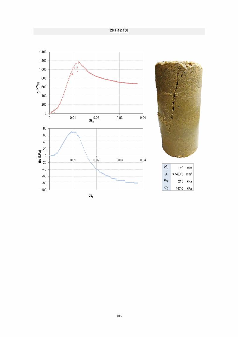
106

28 TR 2 150

0H 140 mm

A 3.74E+3 mm2

cpu 213 kPa

3 147.0 kPa

0

200

400

600

800

1 000

1 200

1 400

0 0.01 0.02 0.03 0.04

q (

KP

a)

dεa

-100

-80

-60

-40

-20

0

20

40

60

80

0 0.01 0.02 0.03 0.04Δu

(kP

a)

dεa

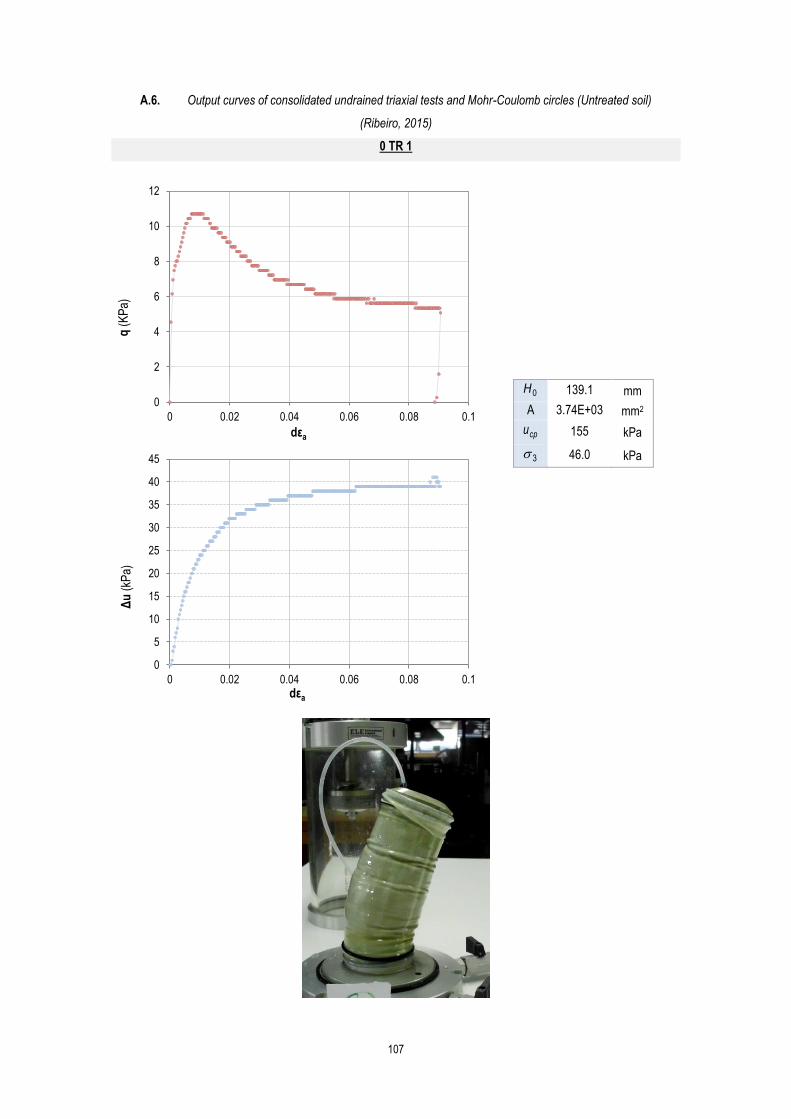
107

A.6. Output curves of consolidated undrained triaxial tests and Mohr-Coulomb circles (Untreated soil)

(Ribeiro, 2015)

0 TR 1

0H 139.1 mm

A 3.74E+03 mm2

cpu

155 kPa

3 46.0 kPa

0

2

4

6

8

10

12

0 0.02 0.04 0.06 0.08 0.1

q (

KP

a)

dεa

0

5

10

15

20

25

30

35

40

45

0 0.02 0.04 0.06 0.08 0.1

Δu

(kP

a)

dεa

108

0 TR 2

0H 137.0 mm

A 3.74E+03 mm2

cpu

165 kPa

3 137.0 kPa

0

20

40

60

80

100

120

140

160

180

0 0.02 0.04 0.06 0.08 0.1 0.12

q (

KP

a)

dεa

0

10

20

30

40

50

60

70

80

0 0.02 0.04 0.06 0.08 0.1 0.12

Δu

(kP

a)

dεa

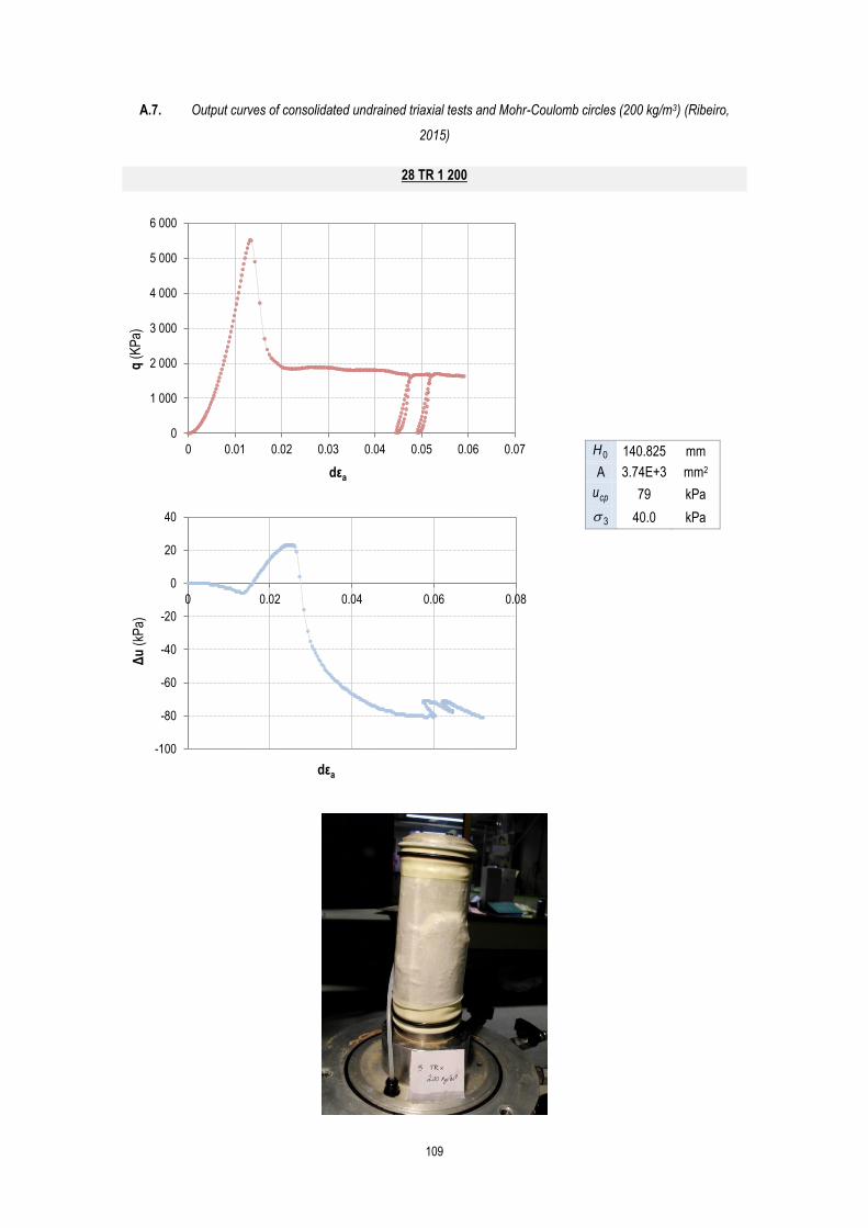
109

A.7. Output curves of consolidated undrained triaxial tests and Mohr-Coulomb circles (200 kg/m3) (Ribeiro,

2015)

28 TR 1 200

0H 140.825 mm

A 3.74E+3 mm2

cpu

79 kPa

3 40.0 kPa

0

1 000

2 000

3 000

4 000

5 000

6 000

0 0.01 0.02 0.03 0.04 0.05 0.06 0.07

q (

KP

a)

dεa

-100

-80

-60

-40

-20

0

20

40

0 0.02 0.04 0.06 0.08

Δu

(kP

a)

dεa

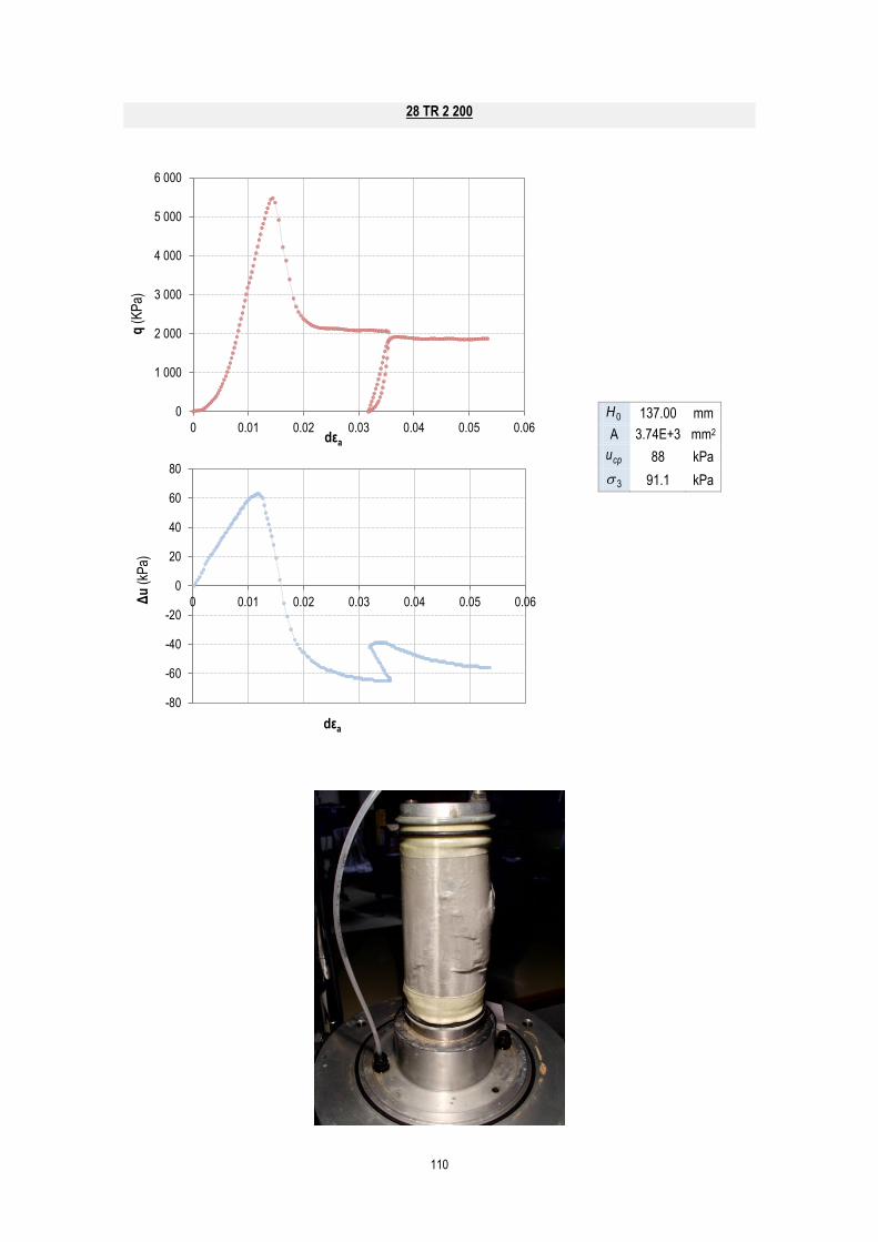
110

28 TR 2 200

0H 137.00 mm

A 3.74E+3 mm2

cpu

88 kPa

3 91.1 kPa

0

1 000

2 000

3 000

4 000

5 000

6 000

0 0.01 0.02 0.03 0.04 0.05 0.06

q (

KP

a)

dεa

-80

-60

-40

-20

0

20

40

60

80

0 0.01 0.02 0.03 0.04 0.05 0.06Δu

(kP

a)

dεa

111

28 TR 3 200

0H 139.1 mm

A 3.74E+3 mm2

cpu

80 kPa

3 158.9 kPa

0

1 000

2 000

3 000

4 000

5 000

6 000

7 000

8 000

0 0.02 0.04 0.06 0.08 0.1

q (

KP

a)

dεa

-100

-80

-60

-40

-20

0

20

40

60

0 0.02 0.04 0.06 0.08 0.1

Δu

(kP

a)

dεa

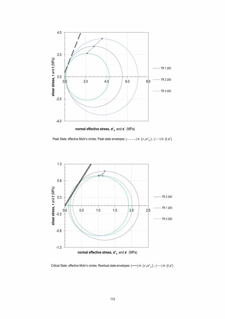
112

Peak State: effective Mohr’s circles. Peak state envelopes: ( ) in )',( n ; ( ) in )',( st

Critical State: effective Mohr’s circles. Residual state envelopes: ( ) in )',( n ; ( ) in )',( st

-4.0

-2.0

0.0

2.0

4.0

0.0 2.0 4.0 6.0 8.0

shea

r st

ress

, τ

and

t (M

Pa)

normal effective stress, σ'n and s' (MPa)

TR 1 200

TR 2 200

TR 3 200

-1.3

-0.8

-0.3

0.3

0.8

1.3

0.0 0.5 1.0 1.5 2.0 2.5

shea

r st

ress

, τ

and

t (M

Pa)

normal effective stress, σ'n and s' (MPa)

TR 2 200

TR 1 200

TR 3 200

113

A.8. Output curves of consolidated undrained triaxial tests and Mohr-Coulomb circles (250 kg/m3) (Ribeiro,

2015)

28 TR 1 250

0H 142.5 mm

A 3.74E+03 mm2

cpu

115 kPa

3 11.0 kPa

0

1 000

2 000

3 000

4 000

5 000

6 000

0 0.01 0.02 0.03 0.04 0.05 0.06 0.07

q (

KP

a)

dεa

-180

-160

-140

-120

-100

-80

-60

-40

-20

0

20

40

0 0.01 0.02 0.03 0.04 0.05 0.06 0.07

Δu

(kP

a)

dεa

114

28 TR 2 250

0H 141.0 mm

A 3.74E+03 mm2

cpu

122 kPa

3 22.5 kPa

0

2 000

4 000

6 000

8 000

10 000

12 000

0 0.01 0.02 0.03 0.04 0.05

q (

KP

a)

dεa

-160

-140

-120

-100

-80

-60

-40

-20

0

20

40

0 0.01 0.02 0.03 0.04 0.05

Δu

(kP

a)

dεa

115

28 TR 3 250

0H 135 mm

A 3.74E+0.3 mm2

cpu

66 kPa

3 58.0 kPa

0

2 000

4 000

6 000

8 000

10 000

12 000

0 0.01 0.02 0.03 0.04 0.05 0.06

q (

KP

a)

dεa

-120

-100

-80

-60

-40

-20

0

20

40

0 0.01 0.02 0.03 0.04 0.05 0.06

Δu

(kP

a)

dεa

116

Peak State: effective Mohr’s circles. Peak states envelope: ( ) in )',( n ; ( ) in )',( st

Critical State: effective Mohr’s circles. Residual state envelopes: ( ) in )',( n ; ( ) in )',( st

-5.0

-3.0

-1.0

1.0

3.0

5.0

0.0 2.0 4.0 6.0 8.0 10.0

shea

r st

ress

, τ

and

t (M

Pa)

normal effective stress, σ'n and s' (MPa)

TR 3 250

TR 1 250

TR 2 250

y = 0.8851x R² = 0.9853

y = 1.9015x

-2.0

-1.5

-1.0

-0.5

0.0

0.5

1.0

1.5

2.0

0.0 1.0 2.0 3.0 4.0

shea

r st

ress

, τ a

nd t

(M

Pa)

normal effective stress, σ'n and s' (MPa)

TR 1 250

TR 2 250

TR 3 250

117

A.9. Saturated permeabilities (Untreated and tretad soil)

150 kg/m3

200 kg/m3 (Ribeiro, 2015)

Δu1 i Δu2 i

kPa - kPa -

100 500.13 200 1000.25

-

t m Q KSAT t m Q kSAT

days g cm3/s m/s days g cm

3/s m/s

3 5.7136 0.38 3.88E-07 3 5.6169 0.37 1.91E-07

3 5.2144 0.35 3.54E-07 3 6.0802 0.41 2.06E-07

3 6.1281 0.41 4.16E-07 3 6.4888 0.43 2.20E-07

7 3.8588 0.26 2.62E-07 7 6.6509 0.44 2.26E-07

7 3.5962 0.24 2.44E-07 7 7.1675 0.48 2.43E-07

7 3.7293 0.25 2.53E-07 7 7.2899 0.49 2.47E-07

14 0.2586 0.02 1.76E-08 14 0.1842 0.01 6.25E-09

14 0.2522 0.02 1.71E-08 14 0.2374 0.02 8.06E-09

14 0.2596 0.02 1.76E-08 14 0.1978 0.01 6.71E-09

28 0.1563 0.01 1.06E-08 28 0.1823 0.01 6.19E-09

28 0.1612 0.01 1.09E-08 28 0.1383 0.01 4.69E-09

28 0.1699 0.01 1.15E-08 28 0.1800 0.01 6.11E-09

Δu1 i Δu2 i

kPa - kPa -

100 500.13 200 1000.25

-

t m Q KSAT t m Q kSAT

days g cm3/s m/s days g cm

3/s m/s

3 2.0398 0.07 6.92E-08 3 2.6950 0.09 4.57E-08

3 2.1561 0.07 7.32E-08 3 2.4759 0.08 4.20E-08

3 1.9718 0.07 6.69E-08 3 3.0752 0.10 5.22E-08

7 2.3087 0.08 7.84E-08 7 2.0122 0.07 3.42E-08

7 2.3253 0.08 7.89E-08 7 2.0760 0.07 3.52E-08

7 2.1882 0.07 7.43E-08 7 1.9806 0.07 3.36E-08

14 2.1657 0.07 7.35E-08 14 2.6460 0.09 4.49E-08

14 2.2878 0.08 7.77E-08 14 2.6886 0.09 4.56E-08

14 2.4193 0.08 8.21E-08 14 2.2999 0.08 3.90E-08

28 1.5933 0.05 5.41E-08 28 1.4690 0.05 2.49E-08

28 1.6406 0.05 5.57E-08 28 1.5913 0.05 2.70E-08

28 1.7276 0.06 5.86E-08 28 1.4966 0.05 2.54E-08

118

250 kg/m3 (Ribeiro, 2015)

Δu1 i Δu2 i

kPa - kPa -

100 500.13 200 1000.25

-

t m Q KSAT t m Q kSAT

days g cm3/s m/s days g cm

3/s m/s

3 0.2720 0.01 9.23E-09 3 0.3055 0.01 5.19E-09

3 0.2474 0.01 8.40E-09 3 0.2945 0.01 5.00E-09

3 0.2423 0.01 8.22E-09 3 0.3017 0.01 5.12E-09

7 0.2357 0.01 8.00E-09 7 0.2488 0.01 4.22E-09

7 0.2322 0.01 7.88E-09 7 0.2297 0.01 3.90E-09

7 0.2369 0.01 8.04E-09 7 0.2436 0.01 4.13E-09

14 0.1208 0.00 4.10E-09 14 0.1489 0.00 2.53E-09

14 0.1256 0.00 4.26E-09 14 0.1322 0.00 2.24E-09

14 0.1294 0.00 4.39E-09 14 0.1620 0.01 2.75E-09

28 0.0741 0.00 2.52E-09 28 0.0845 0.00 1.43E-09

28 0.0741 0.00 2.52E-09 28 0.0794 0.00 1.35E-09

28 0.0675 0.00 2.29E-09 28 0.0797 0.00 1.35E-09

119

A.10. Deviatoric stress-strain curve and excess pore-water pressure development (Ribeiro, 2015)

200 kg/m3

0

1 000

2 000

3 000

4 000

5 000

6 000

7 000

8 000

0 0.01 0.02 0.03 0.04 0.05 0.06 0.07

q (

KP

a)

dεa

28 TR 1 200

28 TR 2 200

28 TR 3 200

σ31=40kPa

σ32=91kPa

σ33=159kPa

-100

-80

-60

-40

-20

0

20

40

60

80

0 0.01 0.02 0.03 0.04 0.05 0.06 0.07

Δu

(K

Pa)

dεa

28 TR 1 200

28 TR 2 200

28 TR 3 200

120

250 kg/m3

0

2 000

4 000

6 000

8 000

10 000

12 000

0 0.01 0.02 0.03 0.04 0.05 0.06

q (

KP

a)

dεa

28 TR 1 250

28 TR 2 250

28 TR 3 250

σ32= 23 kPa

σ31= 11 kPa

σ33= 58 kPa

-160

-140

-120

-100

-80

-60

-40

-20

0

20

40

0 0.01 0.02 0.03 0.04 0.05 0.06

Δu

(K

Pa)

dεa

28 TR 1 250

28 TR 2 250

28 TR 3 250

121

A.11. Stress paths off all the tests, until critical state (Ribeiro, 2015)

200 kg/m3

250 kg/m3

0

1000

2000

3000

4000

5000

6000

7000

8000

0 500 1000 1500 2000 2500 3000

q (

kPa)

p,p' (kPa)

28 TR 1 200

28 TR 2 200

28 TR 3 200

0

2000

4000

6000

8000

10000

12000

0 500 1000 1500 2000 2500 3000 3500

q (

kPa)

p,p' (kPa)

TR 1 250

TR 2 250

TR 3 250

122

A.12. Calibration Curve of the local displacement transducer

SENSITIVITY: 0.003476 mm/mV

y = 287.51x - 2729.8

-2800

-2600

-2400

-2200

-2000

-1800

0 1 2 3

Mea

sure

d v

olt

age

(mV

)

Applied displacement (mm)