Constant-Coe cient Linear Di erential Equationsmoose/240S2013/slides8-05.pdf · We have now learned how to solve homogeneous linear di erential equations P(D) ... a solution to the

Constant-Coefficient

LinearDifferentialEquations

Math 240

Homogeneousequations

Nonhomog.equations

Constant-Coefficient Linear DifferentialEquations

Math 240 — Calculus III

Summer 2013, Session II

Monday, August 5, 2013



Math 240


Nonhomog.equations

Agenda

1. Homogeneous constant-coefficient linear differentialequations

2. Nonhomogeneous constant-coefficient linear differentialequations



Math 240


Nonhomog.equations

Introduction

Last week we found solutions to the linear differential equation

y′′ + y′ − 6y = 0

of the form y(x) = erx. In fact, we found all solutions.This technique will often work. If y(x) = erx then

y′(x) = rerx, y′′(x) = r2erx, . . . , y(n)(x) = rnerx.

So if rn + a1rn−1 + · · ·+ an−1r + an = 0 then y(x) = erx is a

solution to the linear differential equation

y(n) + a1y(n−1) + · · ·+ an−1y

′ + any = 0.

Today we’ll develop this approach more rigorously.



Math 240


Nonhomog.equations

The auxiliary polynomial

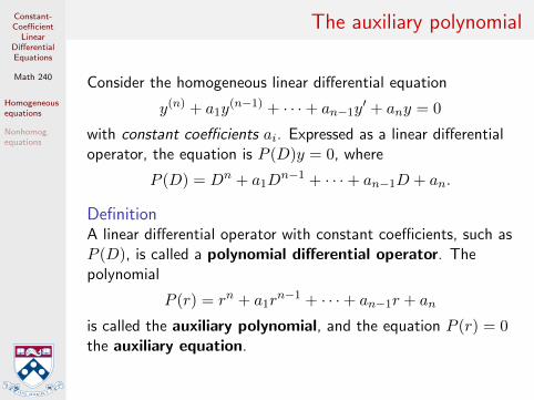
Consider the homogeneous linear differential equation

y(n) + a1y(n−1) + · · ·+ an−1y

′ + any = 0

with constant coefficients ai. Expressed as a linear differentialoperator, the equation is P (D)y = 0, where

P (D) = Dn + a1Dn−1 + · · ·+ an−1D + an.

DefinitionA linear differential operator with constant coefficients, such asP (D), is called a polynomial differential operator. Thepolynomial

P (r) = rn + a1rn−1 + · · ·+ an−1r + an

is called the auxiliary polynomial, and the equation P (r) = 0the auxiliary equation.



Math 240


Nonhomog.equations

The auxiliary polynomial

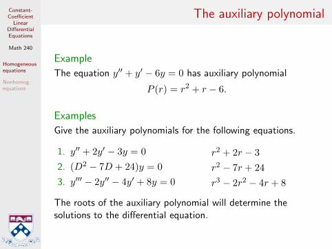
Example

The equation y′′ + y′ − 6y = 0 has auxiliary polynomial

P (r) = r2 + r − 6.

Examples

Give the auxiliary polynomials for the following equations.

1. y′′ + 2y′ − 3y = 0

2. (D2 − 7D + 24)y = 0

3. y′′′ − 2y′′ − 4y′ + 8y = 0

r2 + 2r − 3

r2 − 7r + 24

r3 − 2r2 − 4r + 8

The roots of the auxiliary polynomial will determine thesolutions to the differential equation.



Math 240


Nonhomog.equations

Polynomial differential operators commute

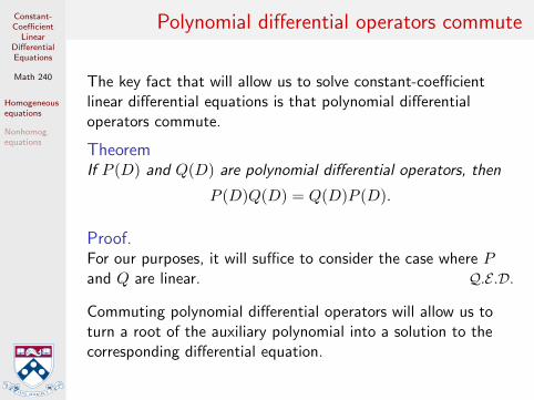
The key fact that will allow us to solve constant-coefficientlinear differential equations is that polynomial differentialoperators commute.

TheoremIf P (D) and Q(D) are polynomial differential operators, then

P (D)Q(D) = Q(D)P (D).

Proof.For our purposes, it will suffice to consider the case where Pand Q are linear. Q.E .D.

Commuting polynomial differential operators will allow us toturn a root of the auxiliary polynomial into a solution to thecorresponding differential equation.



Math 240


Nonhomog.equations

Linear polynomial differential operators

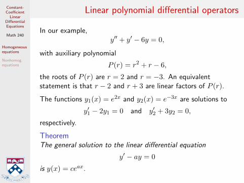
In our example,y′′ + y′ − 6y = 0,

with auxiliary polynomial

P (r) = r2 + r − 6,

the roots of P (r) are r = 2 and r = −3. An equivalentstatement is that r − 2 and r + 3 are linear factors of P (r).

The functions y1(x) = e2x and y2(x) = e−3x are solutions to

y′1 − 2y1 = 0 and y′2 + 3y2 = 0,

respectively.

TheoremThe general solution to the linear differential equation

y′ − ay = 0

is y(x) = ceax.



Math 240


Nonhomog.equations

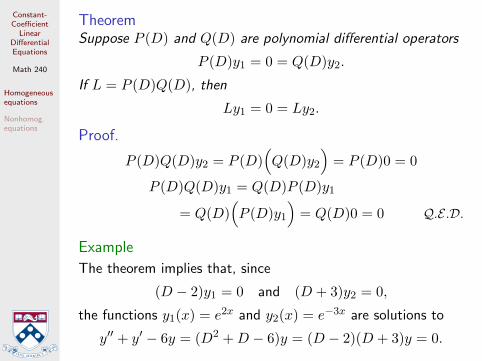
TheoremSuppose P (D) and Q(D) are polynomial differential operators

P (D)y1 = 0 = Q(D)y2.

If L = P (D)Q(D), then

Ly1 = 0 = Ly2.

Proof.

P (D)Q(D)y2 = P (D)(Q(D)y2

)= P (D)0 = 0

P (D)Q(D)y1 = Q(D)P (D)y1

= Q(D)(P (D)y1

)= Q(D)0 = 0 Q.E .D.

Example

The theorem implies that, since

(D − 2)y1 = 0 and (D + 3)y2 = 0,

the functions y1(x) = e2x and y2(x) = e−3x are solutions to

y′′ + y′ − 6y = (D2 +D − 6)y = (D − 2)(D + 3)y = 0.



Math 240


Nonhomog.equations

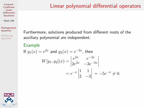
Linear polynomial differential operators

Furthermore, solutions produced from different roots of theauxiliary polynomial are independent.

Example

If y1(x) = e2x and y2(x) = e−3x, then

W [y1, y2](x) =

∣∣∣∣ e2x e−3x

2e2x −3e−3x∣∣∣∣

= e−x∣∣∣∣1 12 −3

∣∣∣∣ = −5e−x 6= 0.



Math 240


Nonhomog.equations

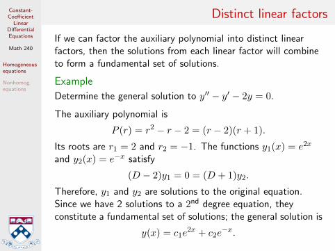
Distinct linear factors

If we can factor the auxiliary polynomial into distinct linearfactors, then the solutions from each linear factor will combineto form a fundamental set of solutions.

Example

Determine the general solution to y′′ − y′ − 2y = 0.

The auxiliary polynomial is

P (r) = r2 − r − 2 = (r − 2)(r + 1).

Its roots are r1 = 2 and r2 = −1. The functions y1(x) = e2x

and y2(x) = e−x satisfy

(D − 2)y1 = 0 = (D + 1)y2.

Therefore, y1 and y2 are solutions to the original equation.Since we have 2 solutions to a 2nd degree equation, theyconstitute a fundamental set of solutions; the general solution is

y(x) = c1e2x + c2e

−x.



Math 240


Nonhomog.equations

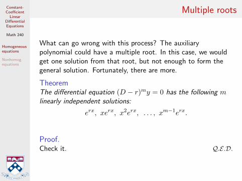
Multiple roots

What can go wrong with this process? The auxiliarypolynomial could have a multiple root. In this case, we wouldget one solution from that root, but not enough to form thegeneral solution. Fortunately, there are more.

TheoremThe differential equation (D − r)my = 0 has the following mlinearly independent solutions:

erx, xerx, x2erx, . . . , xm−1erx.

Proof.Check it. Q.E .D.



Math 240


Nonhomog.equations

Multiple roots

Example

Determine the general solution to y′′ + 4y′ + 4y = 0.

1. The auxiliary polynomial is r2 + 4r + 4.

2. It has the multiple root r = −2.

3. Therefore, two linearly independent solutions are

y1(x) = e−2x and y2(x) = xe−2x.

4. The general solution is

y(x) = e−2x(c1 + c2x).



Math 240


Nonhomog.equations

Complex roots

What happens if the auxiliary polynomial has complex roots?Can we recover real solutions? Yes!

TheoremIf P (D)y = 0 is a linear differential equation with real constantcoefficients and (D − r)m is a factor of P (D) with r = a+ biand b 6= 0, then

1. P (D) must also have the factor (D − r)m,

2. this factor contributes the complex solutions

e(a±bi)x, xe(a±bi)x, . . . , xm−1e(a±bi)x,

3. the real and imaginary parts of the complex solutions arelinearly independent real solutions

xkeax cos bx and xkeax sin bx

for k = 0, 1, . . . ,m− 1.



Math 240


Nonhomog.equations

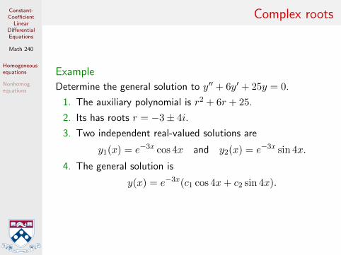
Complex roots

Example

Determine the general solution to y′′ + 6y′ + 25y = 0.

1. The auxiliary polynomial is r2 + 6r + 25.

2. Its has roots r = −3± 4i.

3. Two independent real-valued solutions are

y1(x) = e−3x cos 4x and y2(x) = e−3x sin 4x.


y(x) = e−3x(c1 cos 4x+ c2 sin 4x).



Math 240


Nonhomog.equations

Segue

We have now learned how to solve homogeneous lineardifferential equations

P (D)y = 0

when P (D) is a polynomial differential operator. Now we willtry to solve nonhomogeneous equations

P (D)y = F (x).

Recall that the solutions to a nonhomogeneous equation are ofthe form

y(x) = yc(x) + yp(x),

where yc is the general solution to the associated homogeneousequation and yp is a particular solution.



Math 240


Nonhomog.equations

Overview

The technique proceeds from the observation that, if we knowa polynomial differential operator A(D) so that

A(D)F = 0,

then applying A(D) to the nonhomogeneous equation

P (D)y = F (1)

yields the homogeneous equation

A(D)P (D)y = 0. (2)

A particular solution to (1) will be a solution to (2) that is nota solution to the associated homogeneous equation P (D)y = 0.



Math 240


Nonhomog.equations

Example

Determine the general solution to

(D + 1)(D − 1)y = 16e3x.

1. The associated homogeneous equation is(D + 1)(D − 1)y = 0. It has the general solutionyc(x) = c1e

x + c2e−x.

2. Recognize the nonhomogeneous term F (x) = 16e3x as asolution to the equation (D − 3)y = 0.

3. The differential equation

(D − 3)(D + 1)(D − 1)y = 0

has the general solution y(x) = c1ex + c2e

−x + c3e3x.

4. Pick the trial solution yp(x) = c3e3x. Substituting it into

the original equation forces us to choose c3 = 2.

5. Thus, the general solution is

y(x) = yc(x) + yp(x) = c1ex + c2e

−x + 2e3x.



Math 240


Nonhomog.equations

Annihilators and the method of undeterminedcoefficients

This method for obtaining a particular solution to anonhomogeneous equation is called the method ofundetermined coefficients because we pick a trial solutionwith an unknown coefficient. It can be applied when

1. the differential equation is of the form

P (D)y = F (x),

where P (D) is a polynomial differential operator,

2. there is another polynomial differential operator A(D)such that

A(D)F = 0.

A polynomial differential operator A(D) that satisfiesA(D)F = 0 is called an annihilator of F .



Math 240


Nonhomog.equations

Finding annihilators

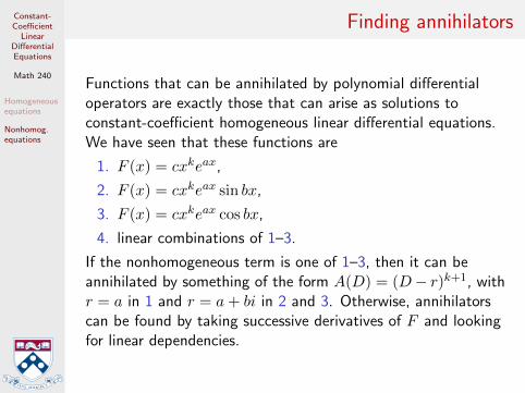
Functions that can be annihilated by polynomial differentialoperators are exactly those that can arise as solutions toconstant-coefficient homogeneous linear differential equations.We have seen that these functions are

1. F (x) = cxkeax,

2. F (x) = cxkeax sin bx,

3. F (x) = cxkeax cos bx,

4. linear combinations of 1–3.

If the nonhomogeneous term is one of 1–3, then it can beannihilated by something of the form A(D) = (D− r)k+1, withr = a in 1 and r = a+ bi in 2 and 3. Otherwise, annihilatorscan be found by taking successive derivatives of F and lookingfor linear dependencies.



Math 240


Nonhomog.equations

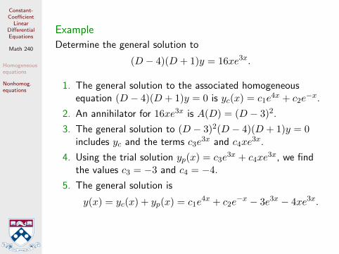
Example


(D − 4)(D + 1)y = 16xe3x.

1. The general solution to the associated homogeneousequation (D − 4)(D + 1)y = 0 is yc(x) = c1e

4x + c2e−x.

2. An annihilator for 16xe3x is A(D) = (D − 3)2.

3. The general solution to (D − 3)2(D − 4)(D + 1)y = 0includes yc and the terms c3e

3x and c4xe3x.

4. Using the trial solution yp(x) = c3e3x + c4xe

3x, we findthe values c3 = −3 and c4 = −4.


y(x) = yc(x) + yp(x) = c1e4x + c2e

−x − 3e3x − 4xe3x.



Math 240


Nonhomog.equations

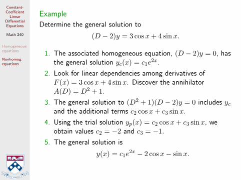
Example


(D − 2)y = 3 cosx+ 4 sinx.

1. The associated homogeneous equation, (D − 2)y = 0, hasthe general solution yc(x) = c1e

2x.

2. Look for linear dependencies among derivatives ofF (x) = 3 cosx+ 4 sinx. Discover the annihilatorA(D) = D2 + 1.

3. The general solution to (D2 + 1)(D − 2)y = 0 includes ycand the additional terms c2 cosx+ c3 sinx.

4. Using the trial solution yp(x) = c2 cosx+ c3 sinx, weobtain values c2 = −2 and c3 = −1.


y(x) = c1e2x − 2 cosx− sinx.

Documents

Constant-Coe cient Linear Di erential Equationsmoose/240S2013/slides8-05.pdf · We have now learned how to solve homogeneous linear di erential equations P(D) ... a solution to the