CONSTRAINING COSMOLOGICAL PARAMETERS AND

TESTING THE ISOTROPY OF THE HUBBLE

EXPANSION USING SUPERNOVAE Ia

Bachelor of Science Thesis

By

Konstantinos Nikolaos Migkas 1

Thesis Supervisor:

Prof. Manolis Plionis

1Physics Department, Aristotle University of Thessaloniki, Thessaloniki

Greece 54124

February, 2015

1

This page intentionally left blank.

Abstract

In this thesis we use the latest Union2.1 Supernovae Ia sample in order to put constraints

to the basic cosmological parameters, such as the Dark Energy equation of state parameter

w , the matter density Ωm and the deceleration parameter q0. We further use the angular

coordinates of the SNe Ia in order to divide the sample in various independent groups,

such as different solid angles, and test the isotropy of the Hubble expansion. Our main

results are:

1. We have reproduced all the published results regarding the cosmological constrains

put by the SNe Ia Hubble expansion probe.

2. We have estimated the deceleration parameter q0 using the low-z SNe Ia (z ≤ 0.24)

and found q0 ' −0.501 corresponding, for a flat Universe, to a matter density

Ωm ' 0.333.

3. We have found that the Ωm-w contours, provided by the SNe Ia analysis of different

redshift ranges, cover distinct regions of the Ωm-w solution space. We have also

found, interestingly, that excluding the intermediate redshift range (0.314 < z ≤

0.57) does not affect significantly the cosmological constraints in the Ωm -w plane,

a fact that can have important implications for future observation strategies.

4. We have identified one sky region, with galactic coordinates 35o < l < 83o &

−79o < b < −37o, containing 82 SNe Ia (15% of total with z ≥ 0.02), that shares a

different Hubble expansion behaviour indicating a possible anisotropy, if confirmed.

We have excluded as a possible cause systematic effects related to the different

surveys that constitute the Union2.1 set. An alternative explanation, that we will

investigate in the future is the existence of a bulk flow that could affect significantly

the redshifts of the specific SNe Ia.

3

Περίληψη

Σε αυτή την εργασία χρησιμοποιούμε το πιο πρόσφατο σετ Υπερκαινοφανών Τύπου Ια

Union2.1 προκειμένου να υπολογίσουμε τα όρια τιμών των βασικών κοσμολογικών παραμέτρων,

όπως ο βαροτροπικός δείκτης w της Σκοτεινής Ενέργειας, η πυκνότητα ύλης Ωm και ο

παράγοντας επιβράδυνσης q0. Επίσης, χρησιμοποιούμε τις γαλαξιακές συντεταγμένες των

Υπερκαινοφανών Ια για να χωρίσουμε το δείγμα σε διάφορες ανεξάρτητες ομάδες, όπως π.χ.

σε στερεές γωνίες, και να ελέγξουμε την ισοτροπία της διαστολής Hubble. Τα βασικά μας

αποτελέσματα είναι:

1. Αναπαράγαμε όλα τα δημοσιευμένα αποτελέσματα που αφορούν τα όρια των κοσ-

μολογικών παραμέτρων που προκύπτουν από τους Υπερκαινοφανείς Ια.

2. Υπολογίσαμε τον συντελεστή επιβράσυνσης q0 χρησιμοποιώντας τους Υπερκαινο-

φανείς Ια με χαμηλές ερυθρομεταθέσεις (z ≤ 0.24) και βρήκαμε q0 ' −0.501, που

αντιστοιχεί, για ένα επίπεδης γεωμετρίας Σύμπαν, σε μια πυκνότητα ύλης Ωm ' 0.333.

3. Βρήκαμε ότι οι ισοπίθανες επιφάνειες των Ωm -w που προκύπτουν από την ανάλυση

των Υπερκαινοφανών Ια για διαφορετικά όρια ερυθρομεταθέσεων, καλύπτουν ανόμοιες

περιοχές στην περιοχή λύσεων των Ωm -w . Επίσης, με πολύ ενδιαφέρον, βρήκαμε ότι

αν αποκλείσουμε τις μεσαίες ερυθρομεταθέσεις (0.314 < z ≤ 0.57, 1/4 του συνο-

λικού δείγματος) δεν επηρεάζονται σημαντικά τα αποτελέσματα και τα όρια των κοσ-

μολογικών παραμέτρων.

4. Ανιχνεύσαμε μία περιοχή του ουρανού με γαλαξιακές συντεταγμένες 35o < l < 83o ·

−79o < b < −37o στην οποία περιέχονται 82 Υπερκαινοφανείς Ια (το 15% του

συνολικού δείγματος με z ≥ 0.02) η οποία χαρακτηρίζεται από μια διαφορετική δι-

αφορά στην διαστολή υποδεικνύοντας μια πιθανή ανισοτροπία στη διαστολή, αν τελικά

επιβεβαιωθεί. Αποκλε;ισαμε ως πιθαν;η αιτ;ια ;ενα συστηματικ;ο σφ;αλμα που σχετ;ιζεται

με διαφορετικο;υς καταλ;ογους δεδομ;ενων τα οπο;ια απαρτ;ιζουν το δε;ιγμα Union2.1 .

Μια εναλλακτική εξήγηση που θα εξετάσουμε στο μέλλον, είναι η ύπαρξη μιας συνεκ-

τικής ροής που θα επηρέαζε τις ερυθρομεταθέσεις των δεδομένων.

4

Acknowledgements

I would like to express my deep gratitude to Prof. Plionis Manolis for guiding and helping

me throughout this thesis. He was always more than willing to spent time with me in

order to solve my queries. His deep knowledge in the field of observational cosmology and

his ideas for this project played a key role in completing it. I am also thankful to Maria

Manolopoulou who provided me with her valuable help about programming tools at the

beginning of my work. Finally, I owe a lot to my lovely girlfriend and fellow student

Eftychia Madika for all her constructive advice, for her daily support and for believing

so much in me.

5

Contents

1 Introduction 8

1.1 Basics of Dynamical Cosmology . . . . . . . . . . . . . . . . . . . . . . . 8

1.2 Taking advantage of standard candles . . . . . . . . . . . . . . . . . . . . 10

1.3 How SNe Ia are produced? . . . . . . . . . . . . . . . . . . . . . . . . . . 12

1.4 The light curves of SNe Ia . . . . . . . . . . . . . . . . . . . . . . . . . . 15

1.5 Cosmic and galactic dust . . . . . . . . . . . . . . . . . . . . . . . . . . . 16

1.6 Other cosmological probes . . . . . . . . . . . . . . . . . . . . . . . . . . 18

2 Theoretical expectations 21

2.1 Different QDE and ΛCDM models comparison . . . . . . . . . . . . . . . 21

2.2 Models comparison for a non-flat Universe (Ωk 6= 0) . . . . . . . . . . . . 23

2.3 Model comparison for CPL parametrization (w = w(z)) . . . . . . . . . . 23

3 The SNe Ia data 26

3.1 Criteria of confirmation of SNe Ia type and quality cuts . . . . . . . . . . 26

3.2 Redshift distribution of the Union2.1 sample . . . . . . . . . . . . . . . . 27

3.3 Mapping the Union2.1 sample . . . . . . . . . . . . . . . . . . . . . . . . 28

3.4 Statistical uncertainties of the distance moduli . . . . . . . . . . . . . . . 32

4 Cosmological parameters fitting 34

4.1 One-parameter models (Ωm or w) . . . . . . . . . . . . . . . . . . . . . . 34

4.2 One-parameter model (q0) . . . . . . . . . . . . . . . . . . . . . . . . . . 35

4.3 Two-parameter model (Ωm and w) . . . . . . . . . . . . . . . . . . . . . 37

4.4 Hubble flow divided in different redshift bins . . . . . . . . . . . . . . . . 40

5 Investigating possible Hubble expansion anisotropies 45

5.1 Among the two galactic hemispheres . . . . . . . . . . . . . . . . . . . . 45

5.2 Among random groups of SNe Ia . . . . . . . . . . . . . . . . . . . . . . 48

6 Joint likelihood analysis 55

6.1 Joint likelihood analysis for the two galactic hemispheres . . . . . . . . . 55

6

6.2 Joint likelihood analysis for the three redshift bins . . . . . . . . . . . . . 56

6.3 Joint likelihood analysis of ten independent SNe Ia subsamples . . . . . . 57

7 Further analysis for the unusual sky region 59

8 Conclusions 65

Appendices 66

A χ2 minimization, our data analysis method 66

B Joint likelihood analysis 68

9 References 69

7

1 Introduction

It is well-known that we live in the Golden Age of Cosmology. The amount of observa-

tional data available is higher than ever. The detailed observations of the cosmos in the

20th century has changed dramatically our ideas for it. Millions of galaxies were discov-

ered, we realized that the Universe is expanding, we found that there are huge amount

of Cold Dark Matter not seen whose nature we still do not know and we predicted and

confirmed the existence of Cosmic Microwave Background (CMB) radiation. However,

maybe the biggest breakthrough of all, was the discovery by Saul Perlmutter, Adam Riess

and Brian P. Schmidt in 1998 that the expansion of the Universe is accelerating, some-

thing completely contrary to what was believed until then. Ever since, the cosmology

community has devoted a large amount of research in order to understand the cause for

the accelerated expansion as well as the nature of the Dark Matter.

1.1 Basics of Dynamical Cosmology

One of the main tools we use to study the dynamical behaviour of the Universe are

the Friedmann equations. Alexander Friedmann in 1922, achieved, using Einstein’s field

equations of gravity to derive a set of equations that described the dynamical behaviour of

the Universe. The content of the Universe is assumed to be a homogeneous perfect fluid,

that is a very good approximation to reality, according to the Cosmological Principle and

the Robertson-Walker metric, which assumes homogeneity and isotropy. Therefore, these

equations describe homogeneous and isotropic FLRW1 models and they are:

H2 =8πGρ

3− kc2

α2+

Λc2

3

H +H2 = −4πG

3

(ρ+

3P

c2

)+

Λc2

3

(1.1)

where H ≡ α

αis the Hubble parameter, with α being the scale factor of the Universe, G

1Friedmann-Lemaıtre-Robertson-Walker

8

the gravitational constant, c the speed of light, ρ the mass density of the total cosmic

(matter and radiation) fluid, Λ the cosmological constant and k = 0,±1 is depended of

the spatial curvature of the Universe. We have k = 0 for a spatially flat Universe and

k = +1,−1 for a positively or negatively curved Universe respectively. Using eq. (1.1)

we can have:

1 =8πGρ

3H2− kc2

α2H2+

Λc2

3H2

=8πG

3H2[ρ+ ρk + ρΛ] ⇒

1 = Ωm + Ωk + ΩΛ

(1.2)

where Ωm, Ωk, ΩΛ are the fractional densities of matter, curvature and the cosmolog-

ical constant or Dark Energy. Dark Energy (hereafter DE) is the term we use for this

hypothetical fluid (with a negative equation of state parameter) that is expressed by ΩΛ

and seems to dominate the Universe in terms of mass-energy density. From eq. (1.1) we

can find the total density (of all source terms mass, radiation, cosmological constant and

curvature), and this is

ρtot =3H2

8πG≈ 10−29 gr/cm3

for this era. Thus, each density parameter is Ωi =ρiρtot

. Combining the two parts of eq.

(1.1) we can derive the continuity equation, that describes the changes of mass-energy

density over time:

ρ+ 3α

α

(ρ+

P

c2

)= 0 ⇒

ρ = −3H

(ρ+

P

c2

)⇒

ρ = −3Hρ(1 + w)

(1.3)

where P = wc2ρ, the equation of state of a perfect fluid and w the equation of state

9

parameter. Finally, we can define the deceleration parameter

q = − ααα2

= −

(1 +

H

H2

)(1.4)

Since 1998, thanks to the work of S. Perlmutter, A. Riess and B. P. Schmidt we know

that q0 < 0, which means that the expansion of the Universe is accelerating, and not

decelerating as would happen if our Universe contained only matter, baryonic or not.

For this to happen, it must be H > 0 or in other words Λ > 0. Generally, the second

derivative of the cosmological scale factor must be α > 0. We have to assume that there

is some form of a perfect fluid, DE, with w < −1/3 in order to have an accelerating

expansion. For baryonic and non-baryonic matter we have w = 0 and for the curvature,

w = −1/3.

From the Friedmann and continuity equations, we can easily derive an equation that

describes how the value of the Hubble parameter depends on the density parameters, the

DE equation of state parameter and redshift z (or time):

H(z) = H0

√Ωm(1 + z)3 + Ωk(1 + z)2 + ΩΛ exp

(3

∫ z

0

1 + w(x)

1 + xdx

)(1.5)

where H0 = 70 km/s/Mpc is the value of the Hubble parameter at this time. The

prevailing values of all these parameters according to the latest data are Ωm ≈ 0.3,

Ωk ≈ 0, ΩΛ ≈ 0.7 and w ≈ −1.

For example, for these exact values, when z = 1 (or 7.7×109 years ago) it was H(z = 1) =

123.2 km/s/Mpc while for a matter-dominant Einstein-de Sitter Universe, it would be

H(z) = 198 km/s/Mpc. Finally, as shown in eq. (1.1), (1.3) and (1.5), for a Λ-dominated

Universe with w = −1, the Hubble parameter would be constant throughout time.

1.2 Taking advantage of standard candles

We characterize as standard candles some astrophysical objects which have a known

constant luminosity which is independent of spatial position and time. This gives as

10

0

100

200

300

400

500

600

700

800

900

1000

1100

0 0.5 1 1.5 2 2.5 3 3.5 4 4.5 5

H(z)

z

w=-1, Ωm=0.3,ΩΛ=0.7

w=0, Ωm=1,ΩΛ=0

w=-1, Ωm=0,ΩΛ=1

Figure 1: . The Hubble parameter as evolves with the redshift for Einstein-de Sitter model

(green dashed line), ΛCDM model (red line) and de Sitter model (blue dashed line).

the huge advantage of knowing the absolute magnitude M of the object. The most

common standard candles are the Cepheid variables and the Supernovae of Type Ia (SNe

Ia). Cepheid variables are used to measure the distances of their host galaxies up to

30 Mpc and to calculate the Hubble constant H0. On the other hand, SNe Ia are used for

cosmological reasons and cosmological distances. If we measure the apparent magnitude

m of a standard candle, then knowing its luminosity means that we know its distance

modulus µ, defined as:

µ = m−M = 5 log dL + 25 (1.6)

where dL is the luminosity distance of the object in Mpc. It is obvious that for standard

candles, since we knowM and we can easily measurem, we can calculate the observational

distance modulus of the object µobs while we also measure the object’s redshift zOn the

other hand, we can theoretically calculate the luminosity distance dL and of course the

distance modulus µth for a given model. For a Universe with a non-flat geometry (Ωk 6= 0),

dL is defined as:

11

dL =c(1 + z)√|Ωk|

sinh

[√|Ωk|

∫ z

0

dx

H(x)

](1.7)

while for a flat Universe (Ωk = 0) is:

dL = c(1 + z)

∫ z

0

dx

H(x)(1.8)

Luminosity distance depends strongly on the cosmological model that we use, since the

Hubble parameter within the integral contains all the cosmological parameters that we

are interested in. Using various methods we can estimate the values of the cosmolog-

ical parameters for which the theoretical expected µth gets as close as possible to the

observational µobs. We analyse the method we use in this thesis, the reduced χ2, in the

Appendix.

1.3 How SNe Ia are produced?

The mechanism that leads to a supernova explosion of type Ia, is thought to be the same,

independent of the time and location of the Universe that it occurs. SNe Ia appear in

binary star systems. When one of the stars consumes all its fuel and thermonuclear fusing

is not possible anymore, the star collapse under its own gravity since thermal pressure

cannot support the outer layers. It passes from several stages of stellar evolution (i.e. red

subgiant, giant etc.) that depend on the star’s original mass. For stars that their mass,

when they enter the main sequence is, M ≤ 5 M their final state is that of an white

dwarf. These are almost the 90% of all known stars.

White dwarfs are the product of the deterrence of the gravitational collapse of a star with

ordinary mass by the pressure of degenerate electrons of its core (Varvoglis, Seiradakis

1994). The interior of the white dwarf mainly consists either of helium (He) for those

with an original star mass of M ≤ 3 M, or of a mix of carbon and oxygen (C-O) for

those with an original star mass of 3 M < M ≤ 5 M. The typical values of mass,

density, radius and temperature of a white dwarf are M ∼ 0.7 M, ρ ∼ 106 gr/cm3,

12

R ∼ 7000 km and T ∼ 106 − 107K respectively. Since the gravitational pressure at the

center of the white dwarf is approximately given by

Pc ≈3

8π

GM2

R4(1.9)

then for M = 1 M and R = 6000 km we obtain Pc ≈ 7.7 × 1022 dyn/cm2. Matter in

the interior of white dwarfs is fully ionized.

Due to the Pauli exclusion principle that states that two identical fermions cannot occupy

the same quantum state at the same time and Heisenberg’s uncertainty principle, that

states ∆x ·∆px ≥ h, with ∆x and ∆px the uncertainties of the position and momentum of

the free particles respectively and h is the Planck constant, the free electrons in the interior

of the white dwarf have a non-zero kinetic pressure. This degenerate electron pressure is

larger than the thermal pressure for more than an order of magnitude. Since the radius

of a white dwarf is inversely proportional to its mass, for high-mass white dwarfs (more

electrons, less space) the space that corresponds to each electron ∆x decreases, so ∆p

and electrons velocity increase. Of course the velocity of the electrons cannot be larger

than the speed of light, so it has an upper limit. For relativistic electrons (high-mass

white dwarfs) the degenerate electron pressure is

Pe =1

8

(3

π

)1/3

hc

(ρ

µemp

)4/3

(1.10)

where mp is the proton mass, µe = A/Z ≈ 2 is the mean molecular weight for a carbon-

oxygen white dwarf, ρ the average density and c the speed of light. For the same values

of mass and radius as before we obtain ρ = 2.2 × 1022 gr/cm3 and thus the degenerate

electron pressure is Pe ≈ 1023 dyn/cm2. As we can see this quantum electron pressure is

capable of resisting the gravitational collapse.

There is a limit of mass though that gravitational pressure becomes so powerful that

degenerate electron pressure is unable to resist it. This mass limit is called Chandrasekhar

limit. Its value can be found by equating the gravitational pressure with the quantum

pressure. For Pc = Pe we obtain a mass limit, independent of the radius R, which is

13

Mch ≈ 1.44 M. A white dwarf cannot have M ≥ Mch. Of course this value of Mch

applies for slow rotating white dwarfs. If someone considers a rapidly rotating white

dwarf, then its mass can exceed this limit, Mch. For a fast rotating C-O white dwarf Mch

is calculated to be 1.8M.

Therefore, in a binary stars system, in which one of the stars becomes a C-O white dwarf,

due to its high density (about 1 million times larger than the Sun’s density), it has a

tremendous gravity. At the surface of a typical white dwarf, we have gWD ≈ 104 gSun,

where gSun is the surface gravity of Sun. Due to the white dwarf’s strong gravitational

field, it can gradually accrete mass from its companion star, which is usually thought to

be a main sequence star, a red giant or a helium star (Yoon and Langer 2004), increasing

its total mass. Since the rate of the accretion is usually M ≥ 10−7 M/yr, this process

can last for about 1 million years. As a result, the C-O white dwarf can finally reach

the critical mass of Mch. The corresponding central density is then ρ ∼ 109 gr/cm3. At

this point, degenerate electron pressure can no longer resist the gravitational collapse.

The white dwarf’s radius decreases rapidly, causing the central pressure to increase and

thermonuclear fusion of burning carbon and oxygen take place in its core. This energy-

producing reactions are:

126 C +12

6 C →2010 Ne+4

2 He+ 4.6 MeV

168 O +16

8 O →2814 Si+4

2 He+ 9.6 MeV

Carbon is the main source of energy since it burns completely, unlike oxygen. The total

energy that is released by these reactions is E ∼ 1044 J , and as a result the star explodes.

This explosion is what we call a Type Ia Supernova (SN Ia). As expected, this large

amount of energy leads to a rapid increase of the luminosity L and correspondingly to

the absolute magnitude M . Since the production mechanism for SNe Ia is always the

same, the peak luminosity of all SNe Ia is considered to be the same, not depending

on time (redshift) and place (coordinates). This is the reason why they are considered

standard candles. Their typical values are L ≈ 5 · 109 L and M ≈ −19.3 ± 0.03 in the

B-band. In many cases, a SN Ia may be even more luminous than its host galaxy.

14

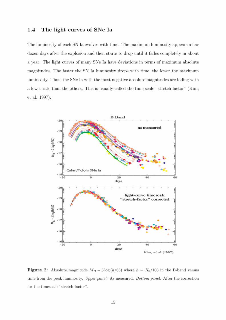
1.4 The light curves of SNe Ia

The luminosity of each SN Ia evolves with time. The maximum luminosity appears a few

dozen days after the explosion and then starts to drop until it fades completely in about

a year. The light curves of many SNe Ia have deviations in terms of maximum absolute

magnitudes. The faster the SN Ia luminosity drops with time, the lower the maximum

luminosity. Thus, the SNe Ia with the most negative absolute magnitudes are fading with

a lower rate than the others. This is usually called the time-scale ”stretch-factor” (Kim,

et al. 1997).

Figure 2: Absolute magnitude MB − 5 log (h/65) where h = H0/100 in the B-band versus

time from the peak luminosity. Upper panel: As measured. Bottom panel: After the correction

for the timescale ”stretch-factor”.

15

In the upper panel of Figure 2 we can see the differences among various SNe Ia light

curves. The vast majority of the light curves lie on the average light curve (the yellow

one). After we stretch (or contract) the time scales of the other light curves and adjust

the peak absolute magnitudes, we get the bottom panel of Figure 2, where all light curves

coincide (Perlmutter et al. 1999).

In order to calculate exactly the correct absolute magnitude, someone have to know the

distance of several SNe Ia by other methods, with great accuracy and measure their max-

imum apparent magnitudes. Then, from eq. (1.6) is easy to find the absolute magnitude

M .

1.5 Cosmic and galactic dust

Interstellar dust is a very important component of the Universe, as it exists in abundance

mostly in spiral galaxies (galactic dust), but there is also a lesser amount of gray dust in

the intergalactic medium (cosmic dust). This dust interacts with the light emitted from

the SNe Ia and causes a reddening of the light we receive since the extinction in the blue

light is much larger. This extinction also causes the dimming of the SNe Ia and, if not

corrected, it can lead to the luminosity distance to be overestimated compared with that

of a Universe that contains no dust (Corasaniti 2006).

After the first indications for an accelerating expansion of the Universe in 1998, the

extinction due to the cosmic gray dust was proposed as the reason for the observing

dimness of the SNe Ia (Aguirre 1999a). This idea has been ruled out in the few next

years for several reasons. First of all, for the Universe to be an Einstein-de Sitter Universe

with Ωm = 1, ΩΛ = 0, it would need to have an intergalactic grey dust density of ΩIGD ≈

5× 10−5 in order to explain the 0.5 mag deviation at z = 0.7 as being due to extinction.

Such a density though, according to Riess et al. (1998), would cause redundant reddening

and light dispersion in the SNe Ia and this is contrary to the observations. In addition,

Perlmutter et al. (1999) found that the intrinsic dispersions at z ≈ 0.05 (from Hamuy et

al. 1996) and z ≈ 0.5 (from Supernova Cosmology Project) were very similar (0.154 ±

0.04 and 0.157 ± 0.025 respectively) and this indicates that the processes that lead to

16

this dispersion are not affected by the redshift (Aguirre 1999b). Moreover, Perlmutter

et al. (1998) studied the mean color difference between low-z and high-z data and

found that they were identical, with |E(B − V )|Hamuy = 0.033 ± 0.014 and |E(B −

V )|SCP = 0.035± 0.022, which shows that there is no significant correlation between the

reddening and the redshift of the SNe Ia. As more SNe Ia discovered with time, the idea

of intergalactic, cosmic dust being responsible for the deviation of the observations from

a matter-dominated Universe was ruled out.

However, intergalactic dust does affect the incoming light of the SNe Ia to a certain

degree. Cosmic dust can consists of grains of several materials and sizes, with lots of

studies (Shustov & Vibe 1995; Davies et al. 1998; Bianchi & Ferrara 2005) suggesting that

these sizes are between 0.02 µm−0.2 µm . Since the extinction due to dust is AB ∼ 1/α,

larger grains mean lesser extinction. Bianchi & Ferrara came to the conclusion that the

distribution of the grains probably remains nearly flat (BF model) while the MRN model

(Mathis, Rumpl, Nordsiek) describes the distribution of these grains as N(α) ∝ α−3.5.

Corasaniti (2006) as well as Menard et al. (2009) and various other studies is find that

the extinction caused by intergalactic dust is about AB ≈ 0.01 mag at z = 0.5 for

graphite and even smaller for silicate. At larger redshifts (z ≈ 1.5) for the BF model we

have AB ≈ 0.08 for graphite at and AB ≈ 0.05 for silicate, while for the MRN model

extinction, it is about 0.02 mag larger for every material. In any case, the deviation in

magnitude is within the uncertainties of the observations. If this extinction is not taken

into account it leads the confidence regions of Dark Energy equation of state parameter

w to more negative values (Corasaniti 2006) and the matter density Ωm to lower values.

If we consider this phenomenon, then the real apparent magnitude mreal that we have to

use in eq. 1.6 is mreal = mobs − AB. So, we calculate a smaller luminosity distance dL

and the values of the constrained cosmological parameters change. Menard et al. (2010)

use the Union sample of SNe Ia to put constraints in cosmological parameters with and

without cosmic dust extinction in order to see how important is the influence of the dust

in the extracted values of the cosmological parameters. They use high-AB(z) and low-

AB(z) extinction models for ΛCDM and Quintessence DE models (hereafter QDE). For

the QDE model, in both extinction cases they find a ∼ 2% shift of Ωm to higher values

17

and a ∼ 2.7% shift of w to less negative values, compared to the parameters extracted in

a dust-free Universe. All these changes are within 0.4σ confidence levels (see the section

below about the statistical analysis method that we use). For the ΛCDM model they

find a shift of δΩm = 0.02 (7.2%) which corresponds to 0.55σ. Finally, Corasaniti (2006)

adopts a cosmic dust model with graphite grains with size of α = 0.1µm in order to study

the shift in the parameters using the Gold SNe Ia sample (Riess et al. 2004) and he finds

a shift of δw = 0.06 (6.25%) that corresponds to 0.38σ.

Except for the intergalactic medium dust, there is another source of extinction, the in-

terstellar medium dust inside the host galaxies of SNe Ia. The SNe Ia that are hosted by

early-type galaxies have a more tight light curve distribution than those hosted by late-

type galaxies (Riess et al. 1999; Sullivan et al. 2006) leading to a very useful uniformity.

This occurs due to the older star populations of early-type galaxies which have a smaller

range of masses than those in the late-type galaxies (Suzuki et al. 2012, hereafter S-12).

However, the SNe Ia colors do not seem to be affected significantly by the type of their

host galaxy.

As known, late-type galaxies contain notably more interstellar dust than early-type ones.

This means that the SNe Ia that are observed in the late galaxies, have smaller statistical

errors and several studies (Sullivan et al. 2003; 2010) have shown that these SNe Ia are

slightly better standard candles than those hosted by late-type galaxies. After correcting

for the color and light curve shape, the SNe Ia in early-type hosts seem to be about

0.14±0.07 mag brighter than those in later types (Hicken et al. 2009c; S-12). This factor

can lead to important systematics errors if not corrected. Finally, SNe Ia in early-type

hosts are more rare since, at lower-z it is observed that one in five SNe Ia occur in an

early-type. (S-12).

1.6 Other cosmological probes

Except for SNe Ia, there are many other probes to study the cosmological parameters,

like the temperature fluctuations of the CMB and Baryon Acoustic Oscillations.

18

Figure 3: The CMB power spectrum as measured by

WMAP until 2006

• CMB radiation is the picture

of our Universe when its age was

about 350, 000 years old, when

photon decoupling occured. It is

almost isotropic, with small tem-

perature fluctuations of ∆T ≈

10−5 K that are considered to

be one of the most powerful cos-

mological probes. The power

spectrum of CMB temperature

anisotropies versus their angular

scale δθ, or multipole moment l,

contains a wealth of cosmological information (Ryden, 2003) since its shape is deter-

mined by oscillations whose amplitudes and positions depend on the Universe’s compo-

sition. For example, the position of the highest peak of the ∆T versus δθ (or l) curve (at

l ≈ 200o, δθ ≈ 0.85o) determines the curvature of the Universe and is consistent with

a spatially flat geometry, k = 0. The characteristic angular scale of the first peak in

the CMB power spectrum is θ =rs(zls)

dA(zls)with rs(zls) is the comoving size of the sound

horizon at last scattering before the photon decoupling and dA(zls) is the comoving an-

gular distance to the last-scattering surface (Davis, Mortsell, Sollerman et al. 2007).

The anisotropies on larger angular scales derive from the influence of the gravitation of

primordial density fluctuations in the Dark Matter distribution (Ryden, 2003). The ratio

of heights between the first and second peaks shows us the amount of baryonic matter.

Generally, using the peaks of the spectrum and using advanced computer simulations to

provide the predictions of different models, we can put constraints in various parameters.

• The BAO provides a characteristic feature in the 2-p correlation function of galaxies,

which results from the interplay between the radiation pressure and gravity in the pho-

tobaryonic plasma, coupled rigidly due to the Thomson scattering in the Universe before

the recombination epoch (Basset, Hlozek, 2009). These two forces impose a system of

standing sound waves within the photon-baryon fluid (Wu et al. 2015). At recombina-

19

tion the pressure on the baryons sharply declines because of the capturing of the free

electrons by the atomic nuclei, and as a result the baryons have small over-densities at

the sound horizon. The corresponding scale is the distance the sound wave had travelled

in the plasma before the recombination (Wu et al. 2015). This distance can be measured

from the CMB to be about 147 Mpc and it can be also measured from the clustering

distribution of galaxies today. Therefore, the BAO scale is what we call a standard ruler.

Standard rulers are cosmological probes with a well known size at a redshift z , or with a

well known way of changing their sizes with redshift. So, by measuring the apparent di-

ameter of the object, we can find the angular distance dA(z) for the given z as well as the

luminosity distance dL(z), and using 1.7 we can constrain the cosmological parameters.

20

2 Theoretical expectations

In order to see how the distance modulus µ depends on the cosmological parameters

and the redshift z, we first compare models with different w and Ωm (we assume a flat

universe, i.e. Ωm + ΩΛ = 1) with a reference ΛCDM model with w = −1 and Ωm = 0.3.

Throughout this whole thesis we use H0 = 70 km/s/Mpc. We also compare models with

Ωk 6= 0 (non-flat Universe) with the same reference model and finally we use models with

the Chevallier-Polarski-Linder (CPL) parametrization of the equation of state parameter.

We define the relative deviations of the distance modulus as

∆µ = µmodel − µΛ (2.1)

where µ is given by eq. (1.6).

2.1 Different QDE and ΛCDM models comparison

To begin with, we first compare cosmological models with different Ωm with the reference

model and then with different w. We firstly use spatially flat models (Ωk = 0). For the

case of a constant w, the Hubble parameter, as we can see in eq. (1.5), is given by

H(z) = H0

√Ωm(1 + z)3 + Ωk(1 + z)2 + ΩΛ(1 + z)3(1+w) (2.2)

We use four different values for each parameter:

As we can see in Figure 4, the relative deviations of the distance moduli in the left panel

are much larger than those in the right panel. That indicates that it is easier to put

limits to the values of Ωm using SNe Ia with z ≥ 1 if we assume a certain value of w,

than limit the values of w for a certain Ωm. This happens because changes in Ωm affect

the luminosity distance (and hence the distance modulus) more strongly than changes in

w.

21

-0.4

-0.3

-0.2

-0.1

0

0.1

0.2

0.3

0.4

0.5

0.01 0.1 1

∆µ

z

Ωm=0.15

Ωm=0.25

Ωm=0.35

Ωm=0.45

-0.08

-0.06

-0.04

-0.02

0

0.02

0.04

0.06

0.08

0.01 0.1 1

∆µ

z

w=-0.85

w=-0.95

w=-1.05

w=-1.15

Figure 4: The expected distance modulus deviations ∆µ vs. z Left panel: Between models

with w = −1 and different Ωm (= 0.15, 0.25, 0.35, 0.45) and the reference model (w = −1,

Ωm = 0.3). Right panel: Between models with Ωm = 0.3 and different w (=

−0.85,−0.95,−1.05,−1.15) and the reference model (w = −1, Ωm = 0.3).

In addition, we can see that in the left panel there is no maximum relative deviation of the

distance moduli. This happens because the first term under the square root containing

Ωm in eq. (2.2) is the most dominant of large redshifts. ∆µ increases with a lower rate

as z increases. The curvature of ∆µ changes at z ≈ 0.9− 1.

In the right panel, the maximum deviation from the reference model occurs at z ≈

1.3 − 1.4. This happens for the same reason as above. The first term under the square

root in H(z) is getting stronger as z increases while the two models have the same Ωm. As

a result, for z ≥ 1.4 any difference in H(z) between the two models begin to eliminate.The

curvature of ∆µ changes at z ≈ 0.5.

As can be derived from Friedmann equations and as shown here, lower values of Ωm and

w correspond to larger luminosity distances for the same z. This means that in a more

”empty” Universe, or in a Universe with a more negative equation of state parameter,

the radial velocity of any light source is lower for the same luminosity distance than in a

Universe with a higher value of Ωm or a less negative w.

22

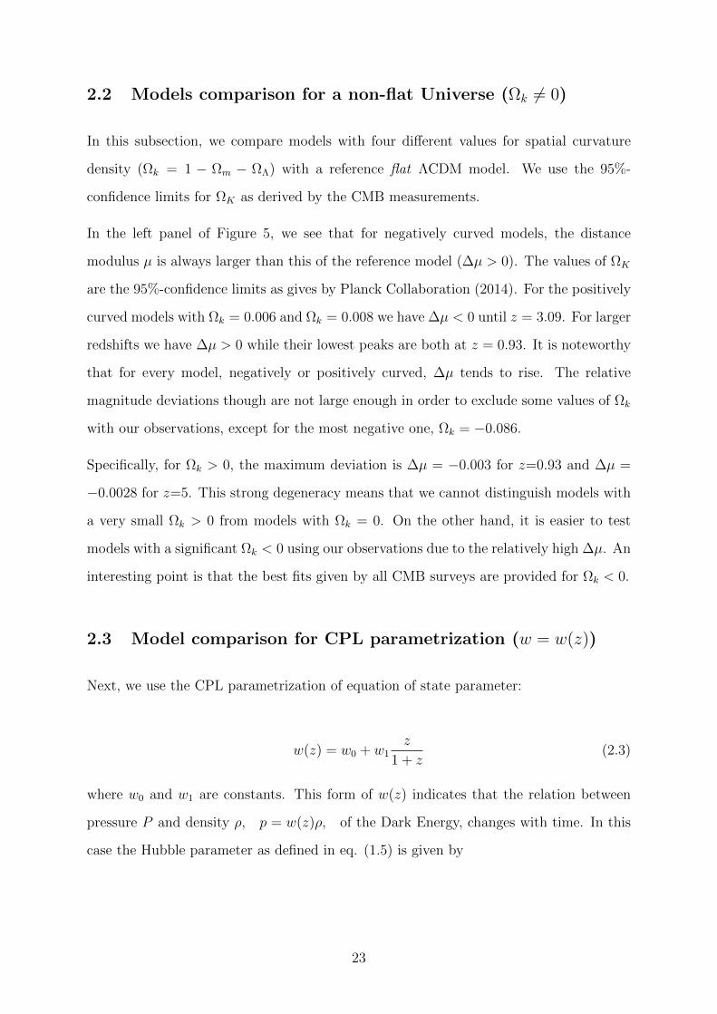
2.2 Models comparison for a non-flat Universe (Ωk 6= 0)

In this subsection, we compare models with four different values for spatial curvature

density (Ωk = 1 − Ωm − ΩΛ) with a reference flat ΛCDM model. We use the 95%-

confidence limits for ΩK as derived by the CMB measurements.

In the left panel of Figure 5, we see that for negatively curved models, the distance

modulus µ is always larger than this of the reference model (∆µ > 0). The values of ΩK

are the 95%-confidence limits as gives by Planck Collaboration (2014). For the positively

curved models with Ωk = 0.006 and Ωk = 0.008 we have ∆µ < 0 until z = 3.09. For larger

redshifts we have ∆µ > 0 while their lowest peaks are both at z = 0.93. It is noteworthy

that for every model, negatively or positively curved, ∆µ tends to rise. The relative

magnitude deviations though are not large enough in order to exclude some values of Ωk

with our observations, except for the most negative one, Ωk = −0.086.

Specifically, for Ωk > 0, the maximum deviation is ∆µ = −0.003 for z=0.93 and ∆µ =

−0.0028 for z=5. This strong degeneracy means that we cannot distinguish models with

a very small Ωk > 0 from models with Ωk = 0. On the other hand, it is easier to test

models with a significant Ωk < 0 using our observations due to the relatively high ∆µ. An

interesting point is that the best fits given by all CMB surveys are provided for Ωk < 0.

2.3 Model comparison for CPL parametrization (w = w(z))

Next, we use the CPL parametrization of equation of state parameter:

w(z) = w0 + w1z

1 + z(2.3)

where w0 and w1 are constants. This form of w(z) indicates that the relation between

pressure P and density ρ, p = w(z)ρ, of the Dark Energy, changes with time. In this

case the Hubble parameter as defined in eq. (1.5) is given by

23

H(z) = H0

√Ωm(1 + z)3 + Ωk(1 + z)2 + ΩΛ(1 + z)3(1+w0+w1) exp

(− 3w1z

1 + z

)(2.4)

-0.02

0

0.02

0.04

0.06

0.08

0.1

0.01 0.1 1

∆µ

z

Ωk=0.006

Ωk=-0.086

Ωk=0.008

Ωk=-0.029

-0.06

-0.04

-0.02

0

0.02

0.04

0.06

0.08

0.1

0.01 0.1 1

∆µ

z

w0=-1, w1=0.3, Ωm=0.28

w0=-1.1, w1=0.3, Ωm=0.27

w0=-0.9, w1=0.1, Ωm=0.3

w0=-1.05, w1=0.2, Ωm=0.31

Figure 5: The expected distance modulus deviations ∆µ vs. z. Left panel: Between

models with (w = −1, Ωm = 0.3) and different Ωk and the reference model (Ωk = 0).

Ωk(= −0.086, 0.006) are the 95%-confidence limits from Planck+WMAP CMB results while

Ωk(= −0.029, 0.008) are the 95%-confidence limits from Planck+WMAP CMB results and

other cosmological probes. Right panel: Between spatially flat models with a combination of

w(z) and Ωm and the reference ΛCDM model (w = −1, Ωm = 0.3)

In the right panel we have four models with a time varying equation of state parameter,

w(z). For a lower w0(= −0.9) value with respect to the reference model and a low positive

w1(= 0.1) (blue-dotted line), it holds that ∆µ < 0 as expected. The lowest peak is again

at z ≈ 1.3, where Ωm starts to play the biggest role in H(z). On the other hand, for

w = −1.1 and for a relatively large w1 = 0.3 (green-dotted line), it holds that ∆µ > 0, but

the lower value of Ωm(= 0.27) has of course to do with this. Maybe the most important

conclusion from the comparison , is the strong degeneracy that exists between the two

other models (red and pink line). There is almost no difference until z = 0.5 and there is

a very small difference of ∆µ ≈ 0.04mag up to z = 5. This is typical of how difficult it is

to differentiate models with w = w(z) instead of a constant w even if Ωm is constrained

with some other cosmological probe. Finally, as we have mentioned several times before,

24

the distance modulus deviations that is caused by different w are reduced as the redshift

increases above some z ∼ 1.5. That causes models with similar Ωm’s to have ∆µ ≈ 0 at

very high z’s (which however is beyond any possibility of obtaining observable data).

25

3 The SNe Ia data

Union2.1 is the most recent compilation of SNe Ia of Supernova Cosmology Project(SCP).

It is the largest one so far, as it first consisted of 833 SNe which were drawn from 19

different datasets. After the lightcurve quality cuts, 580 of them remained. All usability

cuts are developed regardless of cosmological models.

3.1 Criteria of confirmation of SNe Ia type and quality cuts

Only one light curve filter was used for the fitting of Union2.1’s data, the Spectral

Adaptive Light curve Template (SALT2-1). SALT2-1 uses the whole set in order to

calibrate empirical light curve parameters when, at the same time, it typically assumes a

ΛCDM or QDE model. Unfortunately, a model assumption is necessary since it handles

SNe Ia in distances which are larger than those required by the linear Hubble’s law.

However it has been verified that this does not bias the cosmological parameters fit.

As it stated at (S-12) these light curve parameters are

• a colour parameter c, which contains the intrinsic SN colour and reddening due to

dust in its host galaxy (deviation of the mean B − V color of the SN Ia)

• an overall normalization to the time dependent spectral energy distribution (SED)

of a SN Ia, χ0

• the deviation of the average light curve shape, χ1 (or s = χ1 + 1)

The distance modulus is then:

µ = mmaxB −M + αχ1 − βc

with mmaxB the rest-frame peak magnitude in the B-band (P. Smale, 2010) and M the

absolute magnitude in the same band with c = χ1 = 0. Also, SALT2 and SALT2-1 use

α = 0.135 and β = 3.19. The initial light curve standardization results in the best-fitting

values for the time t0 of maximum in the B-band light curves. SNe Ia with observation

time tobs significantly different (several days) from t0 were excluded. In addition, SN Ia

26

candidates which have deviations from the best fit light curve model that are significantly

larger than their uncertainties are rejected.

Some of the high-z SNe that were discovered by the Hubble Space Telescope (HST)

Cluster Supernova Survey, were excluded because they do not have enough information

in their light curves for their type to be determined unambiguously (S-12). SNe that are

SNe Ia, are classified as secure, probable or plausible. A secure SN Ia has a spectrum that

directly confirms that is a SN Ia. Any other SN has to satisfy two conditions: Firstly, its

host galaxy should have spectroscopic, photometric and morphological properties consis-

tent with those of an early-type galaxy with no detectable signs of recent star formation

(S-12), and secondly its light curve shape should be more consistent with that of a SN Ia

and inconsistent with any other known SN types. A probable SN Ia is one that does not

have a secure spectrum but it satisfies one of the above two non-spectroscopic conditions

that are required for a secure classification. Finally, a plausible SN Ia is one that has

an indicative light curve but has not enough information to reject being of other types

(S-12). The Union2.1 further contains 12 secure SNe Ia and 2 probable ones with re-

spect to the Union2, while there are two SNe Ia, one secure (SCP06U4) and one probable

(SCP06K18) that are not included in the Union2.1 sample.

3.2 Redshift distribution of the Union2.1 sample

In this analysis we only use SNe Ia with z ≥ 0.02 in order to avoid uncertainties in

their estimated distances due to the local bulk flow. Thus, we only use the 546 SNe Ia

that have z ≥ 0.02. Union2.1 contains 23 SNe Ia more than the Union2 sample, 21 of

them with z ≥ 0.02 and 10 of them with z > 1. These 10 SNe Ia were discovered by

the Hubble Space Telescope (HST) Cluster Supernova Survey, as well as another 4 SNe

Ia with z ∈ [0.623, 0.973]. Of these 14 SNe Ia, 6 are members of galaxy clusters and

8 are members of non-cluster galaxies. High-redshift SN Ia are extremely important in

calculating the cosmological parameters, because at these redshifts, the differences of the

various DE models are more significant, as we saw in the previous chapter.

From Figure 6 we see that the number of the observed SNe Ia decreases, as expected,

27

0

10

20

30

40

50

60

70

80

90

100

110

120

130

140

150

0 0.1 0.2 0.3 0.4 0.5 0.6 0.7 0.8 0.9 1 1.1 1.2 1.3 1.4 1.5

Fre

quen

cy

z

546 SN Ia events

Figure 6: Redshift distribution of the 546 SNe Ia with z ≥ 0.02 of the Union2.1 sample.

with increasing z. Half of these 546 SNe Ia are for z < 0.316. There are 141 SNe Ia

(25.82% of the sample we use) with z ∈ [0.02, 0.1] while the 141 most distant ones have

z ∈ [0.562, 1.414]. This distribution indicates the need for more high-redshift observa-

tions. Most of the data with z < 0.4 were taken from the Sloan Digital Sky Survey

(SDSS) while most data with z ∈ [0.4, 1] were taken by the SuperNova Legacy Survey

(SNLS). For z > 1, data were taken from the HST survey.

3.3 Mapping the Union2.1 sample

The Union2.1 catalogue contains the name of every SN Ia, its redshift z, the distance

modulus µ, the corresponding 1σ statistical error, σstat, of µ and the probability of each SN

Ia to be a member of a low mass galaxy. It does not contain the equatorial coordinates

(right ascension α and declination δ) of SNe Ia, unlike Union2. However, in order to

calculate the cosmological parameters for different sky regions, we needed the coordinates

of the SNe Ia. Therefore, we took the equatorial coordinates from the Union2 catalogue

for the common SNe Ia with Union2.1, which are 556 (1 SN Ia is excluded from Union2 )

28

and we found the coordinates of the rest SNe Ia from the following websites:

• http://supernova.lbl.gov/2009ClusterSurvey/cands/

• http://www.cbat.eps.harvard.edu/lists/Supernovae.html

• http://astro.berkeley.edu/bait/public html

Knowing the equatorial coordinates of all the Union2.1 SNe Ia, we can produce several

maps of the sample which can help us to visualize its angular distribution. First we make

the polar diagram of all data, with the redshift z being the radius and the right ascension

α being the angle.

1.4

1

0.6

0.2

0.2

0.6

1

1.4

4h

8h

0h

12h

20h

16h

060120180240300

Union2.1 data

Figure 7: Union2.1 data (580 SN Ia events) polar plot for redshift z and right ascension α

As we can see in Figure 7, the higher-z SNe Ia were detected preferentially along various

directions, some of which contain more data than others. For example, there are 97 SNe

Ia for α ∈ [2h, 3h], but there are only 26 SNe Ia for α ∈ [15h, 20h], 22 of them with

z < 0.15.

A more useful representation of the sample’s data is to produce the isosurface plot of the

SNe Ia for α and δ (declination). Doing this, we will be able to see in which regions of

the celestial sphere we have the most data.

29

-90

-80

-70

-60

-50

-40

-30

-20

-10

0

10

20

30

40

50

60

70

80

90

0 1 2 3 4 5 6 7 8 9 10 11 12 13 14 15 16 17 18 19 20 21 22 23 24

Declination

δ (degrees)

Right Ascension α (hours)

-90

-80

-70

-60

-50

-40

-30

-20

-10

0

10

20

30

40

50

60

70

80

90

-180 0 180

Declination

δ (degrees)

Right Ascension α (degrees)

Figure 8: Upper panel: Union2.1 data (580 SN Ia events) plot for equatorial coordinates α

and δ. Bottom panel:The isosurface plot of the sample for α and δ

It is obvious from Figure 7 and Figure 8 that the data distribution is not uniform, since

most SNe Ia have

δ ∈ [−10, 10]. In addition, a lot of them have α ∈ [0h, 4h] ∪ [20h, 24h]1.This happens

because the observational campaigns cover very small solid angles of the sky (cluster of

galaxies etc.), so they detect SNe Ia in tight regions instead of searching the whole sky,

a fact which is dictated by the observational strategies necessary to detect SNe.

1From now on we are going to denote this region as α ∈ [20h, 4h]

30

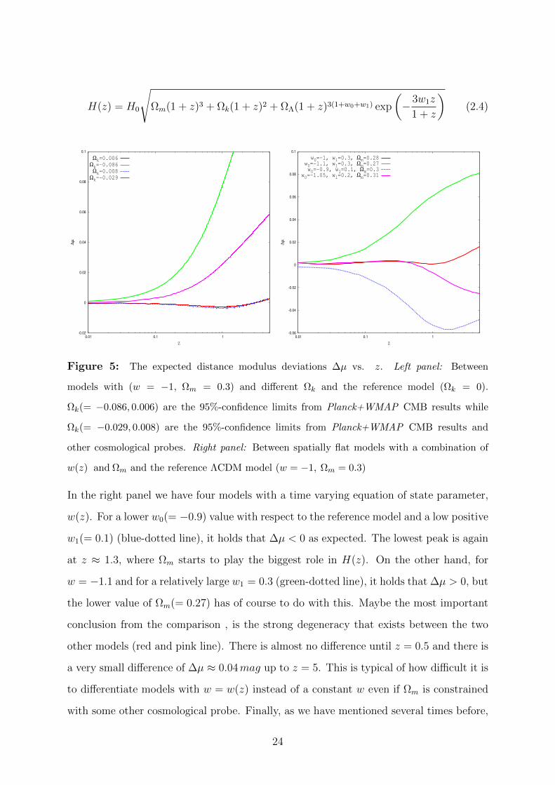
Specifically, there are 263 SNe Ia (45.3% of the sample) within the above δ limits. For

a more narrow sky region with α ∈ [20h, 4h] and δ ∈ [−1.25o, 1.25o] (300 deg2, 0.463%

of the celestial sphere), the SDSS camera was used on the SDSS 2.5m telescope at the

Apache Point Observatory (APO), in order to search for SNe Ia. The observations were

made in the northern fall seasons of 2005 to 2007 (Betoule et al. 2014). That means that

in these limits there are plenty of data with intermediate z’s, as SDSS-II survey targeted

SNe Ia with z ∈ [0.05, 0.4].

We can produce the same plot for the galactic coordinates as well. In order to do that, we

have to convert the equatorial coordinates α and δ into galactic longitude l and galactic

latitude b. For this purpose we use the transformation equations:

l = 33o + arctan

(sin δ sin 62o.6 + cos δ sin (α− 282o.25) cos 62o.6

cos δ cos (α− 282o.25)

)

b = arcsin [sin δ cos 62o.6− cos δ sin (α− 282o.25)]

(3.1)

where all coordinates are in degrees (if α = xh then α = (15x)o).

In Figure 9 we can see that all the data with δ ∈ [−3, 3] from the previous graph, now

form a characteristic ”smile” in the southern galactic hemisphere. There are more data

in the southern galactic hemisphere (351 SNe Ia) than in the northern (229 SNe Ia). As

we mentioned above, we are going to use only the data with z ≥ 0.02, to avoid the local

bulk flow-based uncertainties. With this in mind, we are left with 335 SNe Ia south and

211 SNe Ia north. There are some ”data-rich” areas in the south hemisphere, unlike the

north hemisphere where the observations are more scattered and random.

There are no observations of SNe Ia for b ∈ [−5, 5] due to the Milky way’s plane. The

large amount of dust and gas absorbs the emitted radiation in the optical band, not

allowing us to observe possible SNe Ia.

31

-90

-80

-70

-60

-50

-40

-30

-20

-10

0

10

20

30

40

50

60

70

80

90

0 20 40 60 80 100 120 140 160 180 200 220 240 260 280 300 320 340 360

Galactic latitude b (degrees)

Galactic longtitude l (degrees)

-90

-80

-70

-60

-50

-40

-30

-20

-10

0

10

20

30

40

50

60

70

80

90

0 180 360

Galactic latitude b (degrees)

Galactic longitude l (degrees)

Figure 9: Upper panel: Union2.1 data (580 SN Ia events) plot for galactic coordinates l and

b. Bottom panel: The isosurface of the sample for l and b.

3.4 Statistical uncertainties of the distance moduli

In every analysis of data that are derived from an experiment or observation in any field of

Physics, possible errors or uncertainties of the measurements can affect our conclusions.

In order to have a full perspective of the statistical uncertainties of the distance moduli

µ of the SNe Ia, we present their uncertainty distribution.

In Figure 22, we see that the 1/3 of the data (173 SNe Ia) have a statistical uncertainty

32

0

10

20

30

40

50

60

70

80

90

100

110

120

130

140

150

160

170

180

0.05 0.1 0.15 0.2 0.25 0.3 0.35 0.4 0.45 0.5 0.55 0.6 0.65 0.7 0.75 0.8 0.85 0.9 0.95 1 1.05 1.1

Freq

uenc

y

σstat

σstat for 546 SN Ia events

Figure 10: Statistical uncertainty distribution of the 546 SNe Ia with z ≥ 0.02 of the Union2.1

sample.

of σstat ∈ [0.15, 0.2] while 3/4 of the data (414 SNe Ia) have σstat ∈ [0.1, 0.25]. The mean

value of it is σstat = 0.2229. To compare these statistical errors with their corresponding

distance moduli, we calculate the ratioσstatµ

%. There are only 46 SNe Ia withσstatµ≥ 1%,

and 4 of them haveσstatµ≥ 2%. On the contrary, there are 294 SNe Ia (53.8% of the

sample) withσstatµ≤ 0.5%, 7 of them with

σstatµ≤ 0.25%. Thus, we see that the distance

modulus uncertainties for the Union2.1 sample are minor for the most SNe Ia but there

are exceptions for which the measurement of µ is not very trustworthy.

33

4 Cosmological parameters fitting

4.1 One-parameter models (Ωm or w)

In order to fit our data with a model and extract the best values of the model parameters,

we use the χ2 minimization analysis. We change step-by-step our model parameters values

within some limits and see which combination of them give

χ2 = χ2min. Then, we estimate the uncertainty of these parameters, based on a desired

confidence level. For the whole data analysis part of this thesis, we accept a flat cosmology

and therefore ΩΛ = 1− Ωm.

As a first step in our analysis, we are going to use one free model parameter. To this end,

we initially take p ≡ (Ωm) for a constant w = −1 (ΛCDM) and secondly we use p ≡ (w)

for a constant Ωm = 0.3 (QDE). We use the distance moduli of 546 SNe I (z ≥ 0.02) and

as the error in eq. (A.4), we take the statistical uncertainty, σstat that is provided by the

Union2.1 for each SN Ia.

Since we have one fitted parameter, Nf = 1, our degrees of freedom will be d.o.f. =

546− 1 = 545. From Table 5 we see that for Nf = 1 we have the 1σ (68.3%) confidence

level for ∆χ ≤ 1. Also, the 3σ confidence level is provided for ∆χ ≤ 9. The limits

within which we search for the best-fit values are Ωm ∈ [0, 0.65] for the density matter

and w ∈ [−2,−0.5] for the DE equation of state parameter. Our typical step sizes are

0.001 for Ωm and 0.002 for w.

Our results, as shown in Figure 11, are:

• For w = −1 (fixed):

Ωm = 0.278+0.013−0.014, → χ2

min/d.o.f. = 520.479/545 = 0.955

• For Ωm = 0.3 (fixed):

w = −1.056± 0.032, → χ2min/d.o.f. = 520.593/545 = 0.955

34

1

3

5

7

9

0.239 0.264 0.278 0.291 0.319

χ2-

χ2

min

Ωm

∆χ2 for w=-1

1

3

5

7

9

-1.155 -1.088 -1.056 -1.024 -0.959

χ2-

χ2

min

w

∆χ2 for Ωm=0.3

Figure 11: Left panel: ∆χ2 for Ωm values if w = −1 (fixed). Right panel: ∆χ2 for w if

Ωm = 0.3 (fixed)

We see that our fit in both cases is excellent, with χ2/d.o.f. = 0.955. That shows that

the best pair of values (w,Ωm) is very close to these values. Though, it is more efficient

to fit both parameters at the same time, as we do later. For the 3σ (99.73%) confidence

level (∆χ2 ≤ 9), we have Ωm ∈ [0.239, 0.319] and w ∈ [−1.154,−0.96], limits however

that require the second parameter to be fixed a priori.

4.2 One-parameter model (q0)

We now turn to study the deceleration parameter q0. For low to medium redshifts, we

can use an approximate to eq.(1.8) relation between luminosity distance dL and q0,

dL =c

H0

[z +

1

2(1− q0)z2 + . . .

](4.1)

Using eq.(4.1) and eq.(1.6) we can again apply the χ2 minimization analysis and calculate

q0. Since q is a function of time, q = q(t), we have to use redshifts so as q = q0, i.e. the

parameter value in our epoch. If we use redshifts, for example, z > 0.4, q will not be

approximately constant and our calculations would be wrong. We get the SNe Ia with

35

an increasing zmax with a step size of 0.02, in a range of z ∈ [0.1, 0.36]. For every zmax

we calculate dL and µ for q0 ∈ [−1.5, 0.5] with a step size of 0.001.

-0.9

-0.85

-0.8

-0.75

-0.7

-0.65

-0.6

-0.55

-0.5

-0.45

-0.4

-0.35

-0.3

-0.25

-0.2

-0.15

-0.1

-0.05

0

0.1 0.12 0.14 0.16 0.18 0.2 0.22 0.24 0.26 0.28 0.3 0.32 0.34 0.36

qo

zmax

qo versus zmax with 1σ error bars

Figure 12: Deceleration parameter q0 with 1σ error bars versus the maximum redshift z

until which we take data

As we can see when we plot our results in Figure 12, there are small differences for

different maximum z’s. As we increase zmax, the 1σ error bars get smaller, because

we have more data. For zmax = 0.1, we have 141 SNe Ia and q0 = −0.351+0.249−0.252 with

χ2/d.o.f. = 126.434/140 = 0.903. These large uncertainties (±71% of the best-fit value)

show that we cannot accept a ”safe” mean value of q0. On the other hand, for zmax = 0.24

we have 218 SNe Ia and q0 = −0.501 ± 0.086 with χ2/d.o.f. = 204.738/217 = 0.943. In

this case the 1σ uncertainty is much smaller than the previous (±17%). This is due to

the larger number of data. In both cases, χ2/d.o.f. is very satisfying. It is noteworthy

that none of the uncertainties limits pass to a positive value of q0. Every negative value

of q0 corresponds to a positive acceleration of the scale factor, α > 0. This indicates that

accelerated expansion of our Universe is a robust result even when using limited in z SNe

Ia data.

If we accept that q0 = −0.501 ± 0.086, from the Friedmann equation’s (1.1) and their

derivatives, eq. (1.2) and eq. (1.4), for a flat Universe (k = 0) we have:

36

q0 =Ωm

2− ΩΛ = −0.501⇒

Ωm

2− (1− Ωm) = −0.501± 0.086⇒

Ωm = 0.333± 0.057

(4.2)

The listed uncertainty has been calculated using error propagation, with δΩm =2

3δq0 and

δqo = 0.086. Thus, even if we only use the SNe Ia with z ≤ 0.24, we have a very good

approximation of the matter density Ωm , consistent with the full QDE model results

described below.

4.3 Two-parameter model (Ωm and w)

The main subject of this thesis is to calculate the best-fit values of the QDE cosmological

models, i.e. where p ≡ (w,Ωm), using the reduced χ2 analysis for a group of SNe Ia

data that we choose each time. We also want to plot the solution space within the

1σ uncertainty of our fit and see the limits of the parameters. We use only statistical

uncertainties, σ = σstat, as given in Union2.1 sample. We accept a QDE model of our

Universe.

First, we use the entire sample (546 SNe Ia with z ≥ 0.02) in order to constrain the two

free parameters of the model.

The procedure is as follows: For every w , we use values of the matter density Ωm ∈

[0, 0.65] with a step size of 0.002. When all values of Ωm are tested for a certain w, we

increase w by a step of 0.0025 in a range of w ∈ [−2,−0.5]. Thus, we have 325× 600 =

195, 000 different pairs of p ≡ (w,Ωm) to find the best one. For two fitted parameters,

Nf = 2, the 1σ error corresponds to ∆χ2 ≤ 2.3 while the 3σ error corresponds to

∆χ2 ≤ 11.83. We produce a contour plot that shows the best-fit values and the area

covered in the w and Ωm plane for ∆χ2 ≤ 2.3 and ∆χ2 ≤ 11.83.

In Figure 13 we show the two contours that correspond to the 1σ and 3σ confidence

levels. The corresponding ranges of the 1σ region are: Ωm ∈ [0.17, 0.364] and w ∈

[−1.2425,−0.8]. Moreover, the limits of 99.73% confidence level are: Ωm ∈ [0, 0.448]

37

w

Ωm

∆χ2<11.83

∆χ2<2.3

-2

-1.7

-1.4

-1.1

-0.8

-0.5

0 0.1 0.2 0.3 0.4 0.5 0.6

-1.2425

-1.005

-0.8

0.17 0.28 0.364

Figure 13: Solution space for w and Ωm as it occurs from the analysis of the whole sample

(546 SNe Ia). The blue contour corresponds to the 1σ confidence level (68.3%) and the grey to

the 3σ confidence level (99.73%). The limits of the 1σ confidence level as well as the best-fit

values are shown with the dashed lines.

and w ∈ [−1.61,−0.59]. These values may seem to have huge uncertainties but is very

important to understand the significance of knowing that there is a possibility of 99.73%

for the matter density to be Ωm ≤ 0.448 and the DE equation of state parameter to be

w ≥ −1.61. Of course, not every value of one parameter can be combined with any other

value of the second parameter in 1σ limits. For more negative values of w , Ωm increases

and vice versa.

Table 1: QDE cosmology fits for w and Ωm using all the SNe Ia data (546). When p ≡

(w,Ωm), the uncertainty of each parameter is given by the range for which ∆χ2 ≤ 2.3 while the

other parameter is fixed at its central (best) value.

w Ωm χ2min/d.o.f.

−1.005± 0.045 0.28+0.02−0.018 520.478/544 = 0.956

−1 (fixed) 0.278+0.013−0.014 520.479/545 = 0.955

−1.056± 0.032 0.3 (fixed) 520.593/545 = 0.955

38

The results presented in Table 1 show that our fit is very good, with a reduced χ2min ≈ 1.

The extracted values are very common for nowadays cosmology. Furthermore, we see

that more data mean lower uncertainties, since for the Constitution set (366 SNe Ia with

z ≥ 0.02) the uncertainties are ±0.053 for w and ±0.022 for Ωm (Plionis et al. 2011)

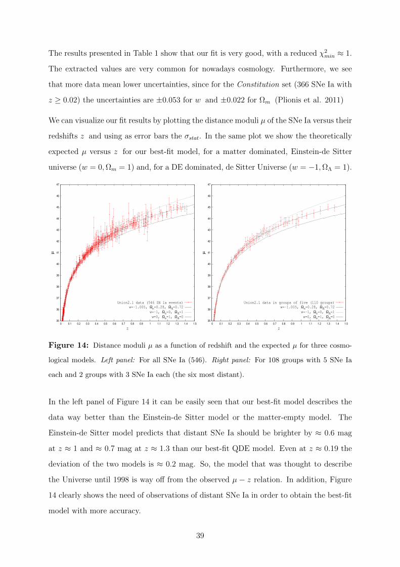
We can visualize our fit results by plotting the distance moduli µ of the SNe Ia versus their

redshifts z and using as error bars the σstat. In the same plot we show the theoretically

expected µ versus z for our best-fit model, for a matter dominated, Einstein-de Sitter

universe (w = 0,Ωm = 1) and, for a DE dominated, de Sitter Universe (w = −1,ΩΛ = 1).

35

36

37

38

39

40

41

42

43

44

45

46

47

0 0.1 0.2 0.3 0.4 0.5 0.6 0.7 0.8 0.9 1 1.1 1.2 1.3 1.4 1.5

µ

z

Union2.1 data (546 SN Ia events)

w=-1.005, Ωm=0.28, ΩΛ=0.72

w=-1, Ωm=0, ΩΛ=1

w=0, Ωm=1, ΩΛ=0 35

36

37

38

39

40

41

42

43

44

45

46

47

0 0.1 0.2 0.3 0.4 0.5 0.6 0.7 0.8 0.9 1 1.1 1.2 1.3 1.4 1.5

µ

z

Union2.1 data in groups of five (110 groups)

w=-1.005, Ωm=0.28, ΩΛ=0.72

w=-1, Ωm=0, ΩΛ=1

w=0, Ωm=1, ΩΛ=0

Figure 14: Distance moduli µ as a function of redshift and the expected µ for three cosmo-

logical models. Left panel: For all SNe Ia (546). Right panel: For 108 groups with 5 SNe Ia

each and 2 groups with 3 SNe Ia each (the six most distant).

In the left panel of Figure 14 it can be easily seen that our best-fit model describes the

data way better than the Einstein-de Sitter model or the matter-empty model. The

Einstein-de Sitter model predicts that distant SNe Ia should be brighter by ≈ 0.6 mag

at z ≈ 1 and ≈ 0.7 mag at z ≈ 1.3 than our best-fit QDE model. Even at z ≈ 0.19 the

deviation of the two models is ≈ 0.2 mag. So, the model that was thought to describe

the Universe until 1998 is way off from the observed µ − z relation. In addition, Figure

14 clearly shows the need of observations of distant SNe Ia in order to obtain the best-fit

model with more accuracy.

39

In the right panel of Figure 14, we group the SNe Ia into groups aggregates in order the

tendencies to be more clearly visible. This is realized by sorting the data in ascending

redshift order and then group every 5 SNe Ia together, starting from the one with the

smallest redshift. The group’s µ, z and σstat are the mean values of the respective quan-

tities of the 5 members of the group. For the last two groups we reduce their membership

into 3 SNe Ia per group in order to have a slightly larger dynamical range in z.

4.4 Hubble flow divided in different redshift bins

In order to test whether the solution space of our parameters change, we dissociate our

data into three bins. The first one has 272 SNe Ia for z ∈ [0.02, 0.314]. The second and

third ones have 137 SNe Ia each and their limits of redshift are z ∈ (0.314, 0.57] and

z ∈ (0.57, 1.414] respectively. We make the space solution for all three bins in order to

find the best-fit values and the 1σ and 3σ confidence levels.

Figure 15 contains some very interesting results. It is obvious that the 1σ contour for

z ∈ (0.57, 1.414] has the lowest uncertainty compared to the two others. This happens

due to the fact that high-z SNe Ia are far more important in constraining the cosmolog-

ical parameters than low-z SNe Ia because the largest model deviations occur at high

redshifts, as it is shown in Figure 4. It is interesting to note that although the lowest-z

subsample has twice as many SNe Ia as the highest-z subsample, and thus one expects

lower random errors, the importance of the high-z regime in constraining the cosmolog-

ical parameters, as described in Section 3, is the factor that provides the most stringent

constraints seen in Figure 15.

However, the size of these contours with respect to the whole sample, are much larger

since they contain 1/4 of the data for z ∈ (0.314, 0.57] and z ∈ (0.57, 1.414] and rela-

tively low redshifts for the first z -range. The 1σ contour range of the fitted parameter

values for the three z -bins are: w ∈ [−2,−0.625], Ωm ∈ [0, 0.578] for the first shell,

w ∈ [−2,−0.615], Ωm ∈ [0, 0.54] for the second shell and w ∈ [−1.665,−0.5575], Ωm ∈

[0, 0.424] for the third shell.

40

w

Ωm

∆χ2<11.83

∆χ2<2.3

-2

-1.7

-1.4

-1.1

-0.8

-0.5

0 0.1 0.2 0.3 0.4 0.5 0.6

-0.6825

0.002

w

Ωm

∆χ2<11.83

∆χ2<2.3

-2

-1.7

-1.4

-1.1

-0.8

-0.5

0 0.1 0.2 0.3 0.4 0.5 0.6

-1.695

0.472

w

Ωm

∆χ2<11.83

∆χ2<2.3

-2

-1.7

-1.4

-1.1

-0.8

-0.5

0 0.1 0.2 0.3 0.4 0.5 0.6

-1.665

-0.9225

0.248 0.424

Figure 15: Solution spaces for w and Ωm The blue contours correspond to the 1σ confidence

level (68.3%) and the grey to the 3σ confidence level (99.73%). Upper left panel: For the 272

SNe Ia with z ∈ [0.02, 0.314]. Upper right panel: For the 137 SNe Ia with z ∈ (0.314, 0.57].

Bottom center panel: For the 137 SNe Ia with z ∈ (0.57, 1.414].

Another interesting fact that is presented in Figure 15 is the variable verticality of the

three contour plots. As the redshift increases, the shape of the contours becomes more

vertical with respect to the Ωm-axes and tend to be more parallel to the w-axes. This

will be more easily visible in the upcoming sections (Figure 24).

In Table 2 we show the best-fit results and their χ2min values for the three different z -bins.

For the first two bins, our best-fit values of w and Ωm seem out of the norm. These

huge differences between them and the best-fit values from the whole sample should be

attributed to the inability to successfully constrain the cosmological parameters when a

41

Table 2: Results of the fits for w and Ωm using the three redshift’s bins SNe Ia data (272,

137 and 137). When p ≡ (w,Ωm), the uncertainty of each parameter is given by the range for

which ∆χ2 ≤ 2.3 when the other parameter is fixed at its central (best) value.

w Ωm χ2min/d.o.f.

First bin, z ∈ [0.02,0.314]

−0.6825+0.055−0.0725 0.002+0.054

−0.002 255.352/270 = 0.946

−1 (fixed) 0.275+0.054−0.052 255.592/271 = 0.943

−1.042± 0.04 0.3 (fixed) 255.639/271 = 0.943

Second bin, z ∈ (0.314,0.57]

−1.695+0.165−0.1775 0.472+0.028

−0.026 117.806/135 = 0.873

−1 (fixed) 0.277+0.038−0.037 118.07/136 = 0.868

−1.052+0.082−0.084 0.3 (fixed) 117.99/136 = 0.868

Third bin, z ∈ (0.57,1.414]

−0.9225+0.06−0.0625 0.248± 0.026 146.761/135 = 1.087

−1 (fixed) 0.279± 0.026 146.81/136 = 1.079

−1.06+0.052−0.054 0.3 (fixed) 146.905/136 = 1.08

sample is dominated by low-z , which lead to a huge degeneracy between models. As we

explained in the previous sections, all the pairs of p ≡ (w,Ωm) within the 1σ contour

plots are of almost equal possibility.

For example, for z = 0.3, the deviation in distance modulus for two models (w,Ωm) =

(−1.005, 0.28) and (w,Ωm) = (−0.6826, 0.002), is ∆µ = 0.007 and for z = 0.5 it becomes

∆µ = 0.034. So, for small samples and low redshifts, models are almost indistinguishable,

42

thus all the combinations of w and Ωm inside the 1σ contour are equally possible.

In order to test how much the SNe Ia with intermediate redshifts affect the final space

solution, we produce the 1σ and 3σ contour plots without the medium redshift bin which

has z ∈ (0.314, 0.57] and contains 137 SNe Ia and we compare it with the solution space

that occurs from the analysis of the whole sample.

w

Ωm

∆χ2<11.83 for the 1

st and 3

rd redshift bins

∆χ2<2.3 for the 1

st and 3

rd redshift bins

-2

-1.7

-1.4

-1.1

-0.8

-0.5

0 0.1 0.2 0.3 0.4 0.5 0.6

-1.2375

-0.985

-0.76

0.148 0.272 0.36

w

Ωm

∆χ2<2.3 for the 1

st and 3

rd redshift bins

∆χ2<2.3 for the Union2.1 sample

-2

-1.7

-1.4

-1.1

-0.8

-0.5

0 0.1 0.2 0.3 0.4 0.5 0.6

-1.005

0.28

Figure 16: Solution spaces for w and Ωm . Left panel: The blue contour corresponds to the

1σ confidence level (68.3%) and the grey to the 3σ confidence level (99.73%) for the 409 SNe

Ia of the 1st and 3rd redshift bins. Right panel: 1σ contours for the whole Union2.1 sample

(red contour) and for the 409 SNe Ia from the 1st and 3rd redshift bins.

As we can see in Figure 16, in this case the resulting solution space is almost identical

with that of the whole sample. It causes just a small shift of the best-fit parameter values

(2.86% for Ωm , 2% for w ) and slightly larger 1σ contours of the parameters. Specifically

we can compare the two solutions below:

• For the joint 1st and 3rd redshift bins:

w = −0.985+0.0525−0.055 , Ωm = 0.272± 0.022 with

χ2min/d.o.f. = 402.398/407 = 0.989 with 1σ corresponding ranges, w ∈ [−1.2375,−0.76],

Ωm ∈ [0.148, 0.36]

43

• For the whole sample:

w = −1.005± 0.045 , Ωm = 0.28+0.02−0.018 with

χ2min/d.o.f. = 520.478/544 = 0.956 with 1σ corresponding ranges, w ∈ [−1.2425,−0.8],

Ωm ∈ [0.17, 0.364]

This probably implies that it is more efficient for future surveys to focus on observing only

low and relatively high redshift standard candles while omitting intermediate redshifts.

44

5 Investigating possible Hubble expansion anisotropies

5.1 Among the two galactic hemispheres

In order to test if there is any anisotropy in expansion between the two galactic hemi-

spheres, we perform the same work as above for each hemisphere separately. First present

the redshift distribution of their data.

0

5

10

15

20

25

30

35

40

45

50

55

60

65

0 0.1 0.2 0.3 0.4 0.5 0.6 0.7 0.8 0.9 1 1.1 1.2 1.3 1.4 1.5

Fre

qu

en

cy

z

335 SN Ia events

0

5

10

15

20

25

30

35

40

45

50

55

60

65

70

75

80

85

0 0.1 0.2 0.3 0.4 0.5 0.6 0.7 0.8 0.9 1 1.1 1.2 1.3 1.4 1.5

Fre

qu

en

cy

z

211 SN Ia events

Figure 17: Redshift distribution of the SNe Ia with z ≥ 0.02. Left panel: Southern galactic

hemisphere (b < 0, 335 SN Ia events) Right panel: Northern galactic hemisphere (b > 0, 211

SN Ia events).

Figure 17 shows us that the redshift distributions of the two galactic hemispheres are quite

distinct. The data of the southern galactic hemisphere are more normally distributed

while in the northern galactic hemisphere there are 82 SNe Ia (39% of the total) with

z < 0.1 and only 9 SNe Ia with 0.1 ≤ z < 0.3. This can make the differentiation of

the fitting cosmological models even harder in the northern galactic hemisphere. This is

because for low redshifts, distance moduli deviations ∆µ between the models are very

small to distinguish and much smaller than the statistical uncertainties. For example, at

z = 0.3 for two models (w,Ωm) = (−0.6, 0) and (w,Ωm) = (−2, 0.6) we have ∆µ = 0.01.

On the other hand, the two galactic hemispheres have similar number of SNe Ia for

z ≥ 0.4, 119 for the southern and 106 for the northern.

45

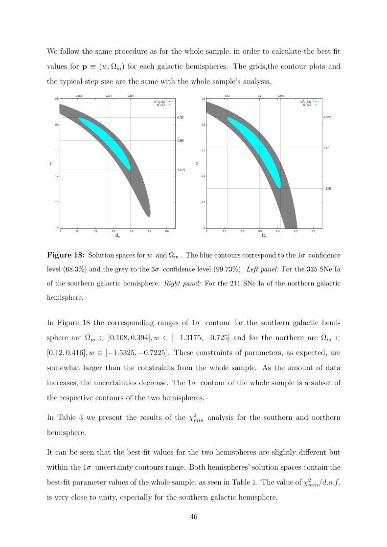
We follow the same procedure as for the whole sample, in order to calculate the best-fit

values for p ≡ (w,Ωm) for each galactic hemispheres. The grids,the contour plots and

the typical step size are the same with the whole sample’s analysis.

w

Ωm

∆χ2<11.83

∆χ2<2.3

-2

-1.7

-1.4

-1.1

-0.8

-0.5

0 0.1 0.2 0.3 0.4 0.5 0.6

-1.3175

-0.985

-0.725

0.108 0.274 0.394

w

Ωm

∆χ2<11.83

∆χ2<2.3

-2

-1.7

-1.4

-1.1

-0.8

-0.5

0 0.1 0.2 0.3 0.4 0.5 0.6

-1.5325

-1.07

-0.7225

0.12 0.3 0.416

Figure 18: Solution spaces for w and Ωm . The blue contours correspond to the 1σ confidence

level (68.3%) and the grey to the 3σ confidence level (99.73%). Left panel: For the 335 SNe Ia

of the southern galactic hemisphere. Right panel: For the 211 SNe Ia of the northern galactic

hemisphere.

In Figure 18 the corresponding ranges of 1σ contour for the southern galactic hemi-

sphere are Ωm ∈ [0.108, 0.394], w ∈ [−1.3175,−0.725] and for the northern are Ωm ∈

[0.12, 0.416], w ∈ [−1.5325,−0.7225]. These constraints of parameters, as expected, are

somewhat larger than the constraints from the whole sample. As the amount of data

increases, the uncertainties decrease. The 1σ contour of the whole sample is a subset of

the respective contours of the two hemispheres.

In Table 3 we present the results of the χ2min analysis for the southern and northern

hemisphere.

It can be seen that the best-fit values for the two hemispheres are slightly different but

within the 1σ uncertainty contours range. Both hemispheres’ solution spaces contain the

best-fit parameter values of the whole sample, as seen in Table 1. The value of χ2min/d.o.f.

is very close to unity, especially for the southern galactic hemisphere.

46

Table 3: Results of fits for w and Ωm using independently the southern and northern galactic

hemispheres’ SNe Ia data (335 and 211 respectively). When p ≡ (w,Ωm), the uncertainty of

each parameter is the range for which ∆χ2 ≤ 2.3 when the other parameter is fixed at its central

(best) value.

w Ωm χ2min/d.o.f.

Southern galactic hemisphere

−0.985± 0.0575 0.274+0.026−0.028 334.588/333 = 1.005

−1 (fixed) 0.28± 0.02 334.594/334 = 1.002

−1.0425± 0.04 0.3 (fixed) 334.664/334 = 1.002

Northern galactic hemisphere

−1.07± 0.08 0.3+0.03−0.028 185.741/209 = 0.889

−1 (fixed) 0.274± 0.02 185.817/210 = 0.885

−1.07+0.052−0.054 0.3 (fixed) 185.741/210 = 0.884

As we did for the whole sample, we plot the distance moduli µ with the statistical

uncertainties σstat versus the redshift of the SNe Ia for each hemisphere as well as the

best-fit models. Moreover, we plot the theoretical distance modulus expectations for the

Einstein-de Sitter and the de Sitter model.

In Figure 19 we see that the best-fit model for each hemisphere predicts almost the same

µ with the best-fit model of the whole sample for z < 1.5. In addition, the lack of data for

0.1 ≤ z < 0.3 in the northern galactic hemisphere is characteristic. Finally, the northern

data contain more ”outliers”, since the SNe Ia in redshifts z = 0.375, 0.55, 0.592 deviate

from the best-fit model by 3.98%, 4.25% and 3.33% respectively. Also, the first two have

the two largest statistical errors of the whole sample (σstat = 0.9232 and σstat = 1.006

respectively) and the third one has the fourth largest error (σstat = 0.718). The third

largest error of the sample belongs to the SN Ia at z = 0.97 of the northern galactic

47

35

36

37

38

39

40

41

42

43

44

45

46

47

0 0.1 0.2 0.3 0.4 0.5 0.6 0.7 0.8 0.9 1 1.1 1.2 1.3 1.4 1.5

µ

z

Southern galactic hemisphere data (335 SN Ia events)

w=-1.005, Ωm=0.28, ΩΛ=0.72

w=-0.985, Ωm=0.274, ΩΛ=0.726

w=-1, Ωm=0, ΩΛ=1

w=0, Ωm=1, ΩΛ=0 35

36

37

38

39

40

41

42

43

44

45

46

47

0 0.1 0.2 0.3 0.4 0.5 0.6 0.7 0.8 0.9 1 1.1 1.2 1.3 1.4 1.5

µz

Northern galactic hemisphere data (211 SN Ia events)

w=-1.005, Ωm=0.28, ΩΛ=0.72

w=-1.07, Ωm=0.3, ΩΛ=0.7

w=-1, Ωm=0, ΩΛ=1

w=0, Ωm=1, ΩΛ=0

Figure 19: SNe Ia distance moduli µ as a function of redshift and the expected µ for four

cosmological models. Left panel: The southern galactic hemisphere’s 335 SNe Ia Right panel:

The northern galactic hemisphere’s 211 SNe Ia.

hemisphere again, which deviates from the best-fit model by 2.8%.

5.2 Among random groups of SNe Ia

In order to test further if there are any anisotropies in the Hubble expansion, we select

four solid angles that contain SNe Ia spanning a large dynamical range in redshift. Two

of them are in the southern galactic hemisphere and the other two in the northern. These

groups are:

• Group A with l ∈ [160, 185] and b ∈ [−63,−50] which contains 82 SNe Ia

• Group B with l ∈ [50, 80] and b ∈ [−70,−38] which contains 53 SNe Ia

• Group C with l ∈ [160, 220] and b ∈ [10, 60] which contains 46 SNe Ia

• Group D with l ∈ [85, 140] and b ∈ [45, 70] which contains 63 SNe Ia

In Figure 20 we present the results of the usual χ2-minimization procedure. We have

used the same step in Ωm and w as before.

48

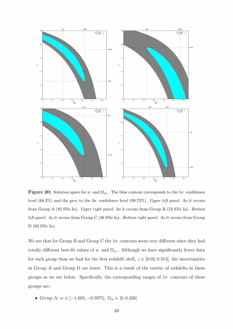
w

Ωm

∆χ2<11.83

∆χ2<2.3

-2

-1.7

-1.4

-1.1

-0.8

-0.5

0 0.1 0.2 0.3 0.4 0.5 0.6

-1.605

-0.9125

0.21 0.426

w

Ωm

∆χ2<11.83

∆χ2<2.3

-2

-1.7

-1.4

-1.1

-0.8

-0.5

0 0.1 0.2 0.3 0.4 0.5 0.6

-2

-0.875

0.234 0.566

w

Ωm

∆χ2<11.83

∆χ2<2.3

-2

-1.7

-1.4

-1.1

-0.8

-0.5

0 0.1 0.2 0.3 0.4 0.5 0.6

-1.5175

-0.65

0 0.418

w

Ωm

∆χ2<11.83

∆χ2<2.3

-2

-1.7

-1.4

-1.1

-0.8

-0.5

0 0.1 0.2 0.3 0.4 0.5 0.6

-1.785

-1.02

0.262 0.434

Figure 20: Solution space for w and Ωm . The blue contour corresponds to the 1σ confidence

level (68.3%) and the grey to the 3σ confidence level (99.73%). Upper left panel: As it occurs

from Group A (82 SNe Ia). Upper right panel: As it occurs from Group B (53 SNe Ia). Bottom

left panel: As it occurs from Group C (46 SNe Ia). Bottom right panel: As it occurs from Group

D (63 SNe Ia).

We see that for Group B and Group C the 1σ contours seem very different since they had

totally different best-fit values of w and Ωm . Although we have significantly fewer data

for each group than we had for the first redshift shell, z ∈ [0.02, 0.314], the uncertainties

in Group A and Group D are lower. This is a result of the variety of redshifts in these

groups as we see below. Specifically, the corresponding ranges of 1σ contours of these

groups are:

• Group A: w ∈ [−1.605,−0.5975], Ωm ∈ [0, 0.426]

49

• Group B: w ∈ [−2,−0.875], Ωm ∈ [0.234, 0.622]

• Group C: w ∈ [−1.5175,−0.555], Ωm ∈ [0, 0.418]

• Group D: w ∈ [−1.785,−0.5875], Ωm ∈ [0, 0.434]

Groups C which has the fewest data, also has the lowest 1σ corresponding range for w,

while its uncertainty for Ωm for every value of w is the highest.

In Table 4 we summarize the results of χ2 analysis for the four data Groups. It is

noteworthy that Groups A and D provide results very near to those of the whole SNe

Ia sample, and they also have the lowest χ2/d.o.f.. Of course, they have the most SNe

Ia compared with the other groups. Even more important is that they also have high-z

data unlike Groups B and C. There is one more interesting observation and is that for

Group B, χ2 for (w,Ωm) = (−1, 0.312) has an important deviation of the best-fit values,

∆χ2 = 1.88. There is no other deviation as large as this for w = −1 (fixed) from χ2min in

this thesis for any other group of data. This may be a hint for a small anisotropy in the

expansion of the Universe for these coordinates, something that we analyse in the next

chapter. In order to see the best-fit models with the corresponding data we produce the

µ vs.z plots for each group.

In Figure 21 we plot the SNe Ia distance moduli µ as a function of redshift z of each

Group. We also plot the best-fit model as it occurs for each Group, the best-fit model

for the whole sample (w,Ωm) = (−1.005, 0.28), the Einstein-de Sitter model and the de

Sitter model. It is evident that Groups A and D have several high-z SNe Ia (z ≥ 1),

while they lack in Groups B and C, with the highest redshift of Group B being z = 0.687

and of Group C being z = 0.882.

In addition, for Groups B and C, the value of χ2min/d.o.f. indicates that the fitted model

is not such a good fit to the data. The main characteristic of Group C is that it contains

the four SNe Ia with the largest uncertainties. The deviations of these distance moduli

∆µ from the theoretically expected µth are quite large. For example, the SN1997l with

z = 0.55 have a deviation of the best-fitted model of ∆µ = 1.795 mag with an uncertainty

of σµ = 1.006. Even for the de Sitter model (w = −1,ΩΛ = 1) it has ∆µ = 1.53 mag. If

50

Table 4: Complete table of fits for w and Ωm using Group A,B,C and D SNe Ia data (82,

53, 46 and 63 respectively). When p ≡ (w,Ωm), the uncertainty of each parameter is the range

for which ∆χ2 ≤ 2.3 when the other parameter is fixed at its central (best) value.

w Ωm χ2min/d.o.f.

Group A, l ∈ [160,185],b ∈ [−63,−50]

−0.9125+0.085−0.0875 0.21+0.048

−0.044 64.6/80 = 0.808

−1 (fixed) 0.253± 0.044 64.66/81 = 0.798

−1.11± 0.04 0.3 (fixed) 65.879/81 = 0.813

Group B, l ∈ [50,80],b ∈ [−70,−38]

−2+0.366 0.566± 0.054 60.02/51 = 1.177

−1 (fixed) 0.312+0.09−0.085 61.9/52 = 1.19

−0.996± 0.0168 0.3 (fixed) 61.938/52 = 1.214

Group C, l ∈ [160,220],b ∈ [10,60]

−0.65± 0.095 0+0.108 49.52/44 = 1.125

−1 (fixed) 0.248+0.088−0.079 50.3/45 = 1.12

−1.096+0.16−0.214 0.3 (fixed) 50.6/45 = 1.127

Group D, l ∈ [85,140],b ∈ [45,70]

−1.02± 0.095 0.262+0.042−0.039 54.779/61 = 0.898

−1 (fixed) 0.257+0.043−0.039 48.023/62 = 0.775

−1.116+0.118−0.126 0.3 (fixed) 48.09/62 = 0.776

51

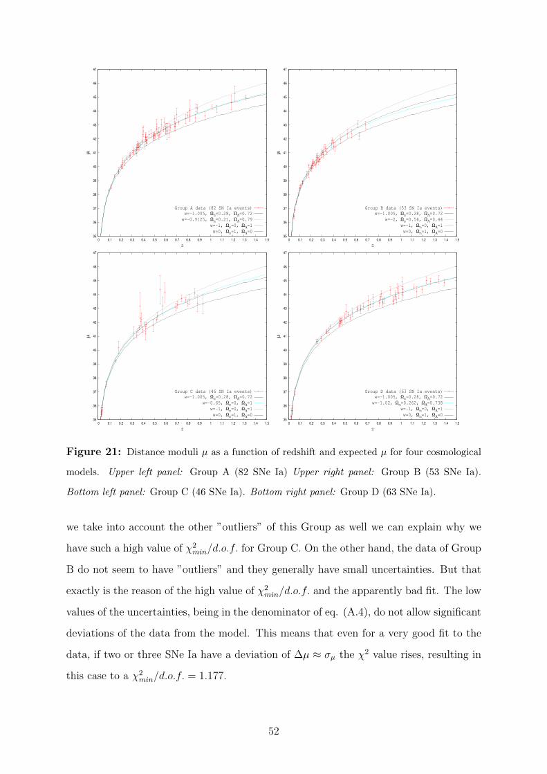
35

36

37

38

39

40

41

42

43

44

45

46

47

0 0.1 0.2 0.3 0.4 0.5 0.6 0.7 0.8 0.9 1 1.1 1.2 1.3 1.4 1.5

µ

z

Group A data (82 SN Ia events)

w=-1.005, Ωm=0.28, ΩΛ=0.72

w=-0.9125, Ωm=0.21, ΩΛ=0.79

w=-1, Ωm=0, ΩΛ=1

w=0, Ωm=1, ΩΛ=0 35

36

37

38

39

40

41

42

43

44

45

46

47

0 0.1 0.2 0.3 0.4 0.5 0.6 0.7 0.8 0.9 1 1.1 1.2 1.3 1.4 1.5

µ

z

Group B data (53 SN Ia events)

w=-1.005, Ωm=0.28, ΩΛ=0.72

w=-2, Ωm=0.56, ΩΛ=0.44

w=-1, Ωm=0, ΩΛ=1

w=0, Ωm=1, ΩΛ=0

35

36

37

38

39

40

41

42

43

44

45

46

47

0 0.1 0.2 0.3 0.4 0.5 0.6 0.7 0.8 0.9 1 1.1 1.2 1.3 1.4 1.5

µ

z

Group C data (46 SN Ia events)

w=-1.005, Ωm=0.28, ΩΛ=0.72

w=-0.65, Ωm=0, ΩΛ=1

w=-1, Ωm=0, ΩΛ=1

w=0, Ωm=1, ΩΛ=0 35

36

37

38

39

40

41

42

43

44

45

46

47

0 0.1 0.2 0.3 0.4 0.5 0.6 0.7 0.8 0.9 1 1.1 1.2 1.3 1.4 1.5

µ

z

Group D data (63 SN Ia events)

w=-1.005, Ωm=0.28, ΩΛ=0.72

w=-1.02, Ωm=0.262, ΩΛ=0.738

w=-1, Ωm=0, ΩΛ=1

w=0, Ωm=1, ΩΛ=0

Figure 21: Distance moduli µ as a function of redshift and expected µ for four cosmological

models. Upper left panel: Group A (82 SNe Ia) Upper right panel: Group B (53 SNe Ia).

Bottom left panel: Group C (46 SNe Ia). Bottom right panel: Group D (63 SNe Ia).

we take into account the other ”outliers” of this Group as well we can explain why we

have such a high value of χ2min/d.o.f. for Group C. On the other hand, the data of Group

B do not seem to have ”outliers” and they generally have small uncertainties. But that

exactly is the reason of the high value of χ2min/d.o.f. and the apparently bad fit. The low

values of the uncertainties, being in the denominator of eq. (A.4), do not allow significant

deviations of the data from the model. This means that even for a very good fit to the

data, if two or three SNe Ia have a deviation of ∆µ ≈ σµ the χ2 value rises, resulting in

this case to a χ2min/d.o.f. = 1.177.

52

For the Groups A and D, the fit of the data are quite satisfying. Especially for Group D,

the best-fit values are very close to the best-fit model from the whole sample, (w,Ωm) =

(−1.005, 0.28). Furthermore, the deviations of distance moduli of the models for these

Groups compared to those from the whole sample, are very small even for z = 1.5 (for

Group D, ∆µ = 0.038). In contrast, the deviations ∆µ for the best-fit models to the

data of Groups B and C are larger at high redshifts (∆µ = −0.26 and ∆µ = 0.223 for

z = 1.5 respectively) but insignificant at the redshift range covered by the data. If there

is any anisotropy in the expansion of the Universe for these directions, it is not easily

seen, although the results based on Group B (l ∈ [50, 80] and b ∈ [−70,−38]) have the

most distinct 1σ contour in the Ωm -w place with respect to all the other Groups.

To find out if this peculiarity of the solution space of Group B is a result of the low-z

data, we also find the solution space for the data of Group A but for the same upper-z

limit (z ≤ 0.689). We also find the solution space for the whole Union2.1 sample after

limiting its redshift to the same upper-z limit (z ≤ 0.689).

w

Ωm

∆χ2<2.3 for the Group A data with z<0.689

∆χ2<2.3 for Group B

-2

-1.7

-1.4

-1.1

-0.8

-0.5

0 0.1 0.2 0.3 0.4 0.5 0.6

-1.32

0.382

w

Ωm

∆χ2<2.3 for Group B

∆χ2<2.3 for Union2.1 data with z<0.689

-2

-1.7

-1.4

-1.1

-0.8

-0.5

0 0.1 0.2 0.3 0.4 0.5 0.6

-1.12

0.334

Figure 22: 1σ contour plots of the Ωm -w plane. Left panel: As they occur from data from

Group A with z ≤ 0.689 (blue contour, 67 SNe Ia) and Group B (red contour, 53 SNe Ia). Right

panel: As they occur from Union2.1 with z ≤ 0.689 (blue contour, 453 SNe Ia) and Group B

(red contour, 53 SNe Ia).

53

In Figure 22 we see that if we use only the data with z ≤ 0.689, the best-fit values come

closer to those of Group B than before. For clarity, we use only the 1σ contour plots. For

Group A, we have (w,Ωm) = (−1.32, 0.382) with χ2min/d.o.f. = /65 = and for Union2.1

we have (w,Ωm) = (−1.12, 0.334) with χ2min/d.o.f. = 427.433/451 = 0.948. Although

there is a significant overlapping between the 1σ contours, especially for Group A, the

difference of the solution space for the same maximum redshift appears still important.

Thus, constraining the upper redshift limit brings the results based on Group B closer to

those of Group A and of the whole sample but still there is significant discrepancies.

54

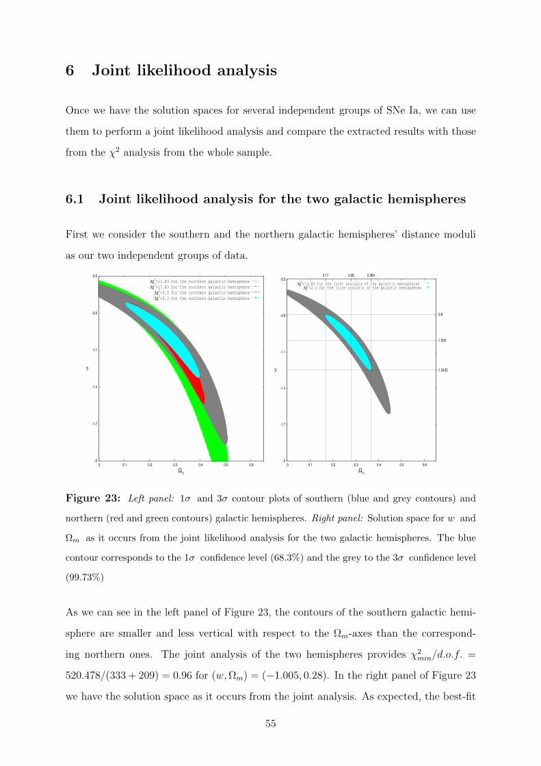
6 Joint likelihood analysis

Once we have the solution spaces for several independent groups of SNe Ia, we can use

them to perform a joint likelihood analysis and compare the extracted results with those

from the χ2 analysis from the whole sample.

6.1 Joint likelihood analysis for the two galactic hemispheres

First we consider the southern and the northern galactic hemispheres’ distance moduli

as our two independent groups of data.

-2

-1.7

-1.4

-1.1

-0.8

-0.5

0 0.1 0.2 0.3 0.4 0.5 0.6

w

Ωm

∆χ2<11.83 for the northern galactic hemisphere

∆χ2<11.83 for the southern galactic hemisphere

∆χ2<2.3 for the northern galactic hemisphere

∆χ2<2.3 for the southern galactic hemisphere

w

Ωm

∆χ2<11.83 for the joint analysis of the galactic hemispheres ∆χ

2<2.3 for the joint analysis of the galactic hemispheres

-2

-1.7

-1.4

-1.1

-0.8

-0.5

0 0.1 0.2 0.3 0.4 0.5 0.6

-1.2425

-1.005

-0.8

0.17 0.28 0.364

Figure 23: Left panel: 1σ and 3σ contour plots of southern (blue and grey contours) and

northern (red and green contours) galactic hemispheres. Right panel: Solution space for w and

Ωm as it occurs from the joint likelihood analysis for the two galactic hemispheres. The blue

contour corresponds to the 1σ confidence level (68.3%) and the grey to the 3σ confidence level

(99.73%)

As we can see in the left panel of Figure 23, the contours of the southern galactic hemi-

sphere are smaller and less vertical with respect to the Ωm-axes than the correspond-

ing northern ones. The joint analysis of the two hemispheres provides χ2min/d.o.f. =

520.478/(333 + 209) = 0.96 for (w,Ωm) = (−1.005, 0.28). In the right panel of Figure 23

we have the solution space as it occurs from the joint analysis. As expected, the best-fit

55

values, the corresponding ranges of 1σ and 3σ contours as well as the value of χ2min are

exactly the same with these from the full sample analysis. The only difference is that the

d.o.f. are reduced and the χ2min/d.o.f. is closer to unity than before.

6.2 Joint likelihood analysis for the three redshift bins

The next subdivisions of the sample that we are going to use are the three redshift bins

as they defined before. The first bin contains 272 SNe Ia for z ∈ [0.02, 0.314], the second

contains 137 SNe Ia for z ∈ (0.314, 0.57] and finally the third also contains 137 SNe Ia,

for z ∈ (0.57, 1.414].

w

Ωm

∆χ2<2.3 for the first redshift shell (0.02<z<0.314)

∆χ2<2.3 for the second redshift shell (0.314<z<0.57)

∆χ2<11.83 for the third redshift shell (z>0.57)

-2

-1.7

-1.4

-1.1

-0.8

-0.5

0 0.1 0.2 0.3 0.4 0.5 0.6

w

Ωm

∆χ2<11.83 for the joint analysis of the 3 redshift shells ∆χ

2<2.3 for the joint analysis of the 3 redshift shells

-2

-1.7

-1.4

-1.1

-0.8

-0.5

0 0.1 0.2 0.3 0.4 0.5 0.6

-1.2475

-1.01

-0.8025

0.172 0.282 0.366

Figure 24: Left panel: 1σ contour plots of the three redshift bins (for clarity we do not

plot any other contours). Right panel: Solution space for w and Ωm as it occurs from the

joint likelihood analysis for the three redshift bins. The blue contour corresponds to the 1σ

confidence level (68.3%) and the grey to the 3σ confidence level (99.73%)

From this joint analysis, the results are slightly different from those from the whole sample

due to round-up errors. The values with the lowest χ2 are (w,Ωm) = (−1.01, 0.282)

with χ2min/d.o.f. = 520.735/(270 + 135 + 135) = 0.964. The best-fits values and the

uncertainties of them when one parameter is fixed are the same with these from the

whole sample. The best-fit combination for the whole sample (w,Ωm) = (−1.005, 0.28)

56

have a deviation of ∆χ2 = 6.6× 10−4, being almost an equally good fit that is extracted

by the joint analysis. Indeed, it is the combination with the lowest ∆χ2 of all.

As we mentioned before for higher redshifts the corresponding contours are more vertical

to the Ωm-axes. Also, we see more clearly that the third and more distant redshift bin

provides the smallest size contour region, although has half the data of the first bin. This

is an excellent indication of the importance of the high-z data.

6.3 Joint likelihood analysis of ten independent SNe Ia subsam-

ples

In order to identify possible anisotropies of the Hubble expansion, we now divide the

Union2.1 sample in 10 fully independent SNe Ia subsamples. Except for the Groups

A,B,C and D we also have:

• Group E with l ∈ [245, 360] and b ∈ [10, 80] with 56 SNe Ia

• Group F with l ∈ [90, 158] and b ∈ [−70,−50] with 68 SNe Ia

• Group G with l ∈ [25, 80] and b ∈ [−35, 90] with 47 SNe Ia

• Group H with l ∈ [81, 215] and b ∈ [−50,−5] which contains 54 SNe Ia

• Group K with l ∈ [30, 45, ] and b ∈ [−90,−40] with 22 SNe Ia

• Group M with all the remaining 55 SNe Ia

We do not use letters ”I, J, L” because they can be mistaken with ”1” and with each

other. Group K has the fewest data but it has important, high-z data with a mean

redshift of z = 0.6847.

In section 5 we pointed out the peculiarity of the solution space provided by Group B.

Since Group K is very near to Group B in galactic coordinates (Figure 9), we join the

two Groups (B and K) in one group and calculate again the solution space of w and

ΩmThe area of these groups in celestial coordinates is between α ∈ [21.2h, 23.94h] and

δ ∈ [−26.36o, 13.46o]. We have to mention here that Group K alone gives similar best-fit

57

values (w = −2,Ωm = 0.51) with Group B and the fact that it has the closest coordinates

to Group B is a strong hint for a consistent behaviour of this whole region.

The best-fit values of the cosmological parameters provided by the joint B+K subsample

are w = −1.7025+0.25−0.275 and Ωm = 0.498+0.042

−0.04 while the 1σ ranges are: w ∈ [−2,−0.8825]

and Ω ∈ [0.262, 0.574]. However due to the degeneracy of the solution, the best-fit

parameters of the whole SNe Ia sample are not included within the 1σ contour provided

by the B+K group.

When we exclude every other Group from the whole sample, the solution spaces does not

change significantly. This means that the 1σ contours for all Groups except for B and

K, are consistent with the results of the rest of the data.

58

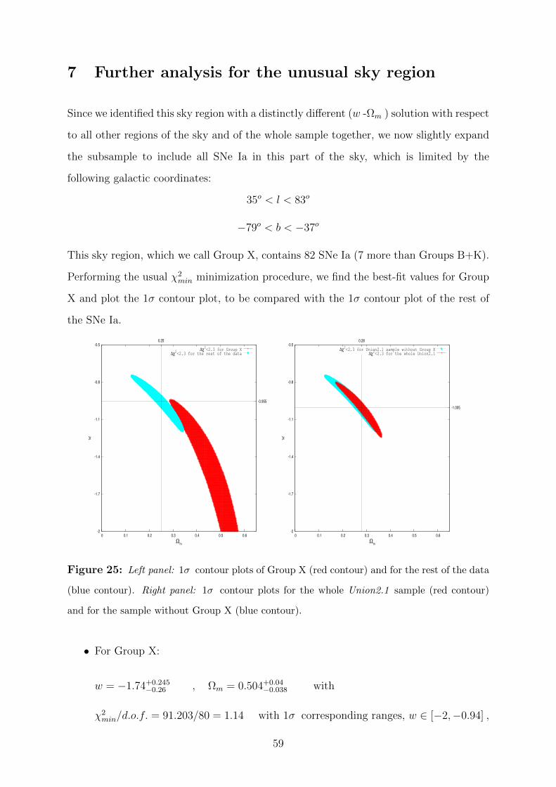
7 Further analysis for the unusual sky region

Since we identified this sky region with a distinctly different (w -Ωm ) solution with respect

to all other regions of the sky and of the whole sample together, we now slightly expand

the subsample to include all SNe Ia in this part of the sky, which is limited by the

following galactic coordinates:

35o < l < 83o

−79o < b < −37o

This sky region, which we call Group X, contains 82 SNe Ia (7 more than Groups B+K).

Performing the usual χ2min minimization procedure, we find the best-fit values for Group

X and plot the 1σ contour plot, to be compared with the 1σ contour plot of the rest of

the SNe Ia.

w

Ωm

∆χ2<2.3 for Group X

∆χ2<2.3 for the rest of the data

-2

-1.7

-1.4

-1.1

-0.8

-0.5

0 0.1 0.2 0.3 0.4 0.5 0.6

-0.955

0.25

w

Ωm

∆χ2<2.3 for Union2.1 sample without Group X

∆χ2<2.3 for the whole Union2.1

-2

-1.7

-1.4

-1.1

-0.8

-0.5

0 0.1 0.2 0.3 0.4 0.5 0.6

-1.005

0.28

Figure 25: Left panel: 1σ contour plots of Group X (red contour) and for the rest of the data

(blue contour). Right panel: 1σ contour plots for the whole Union2.1 sample (red contour)

and for the sample without Group X (blue contour).

• For Group X:

w = −1.74+0.245−0.26 , Ωm = 0.504+0.04

−0.038 with

χ2min/d.o.f. = 91.203/80 = 1.14 with 1σ corresponding ranges, w ∈ [−2,−0.94] ,

59

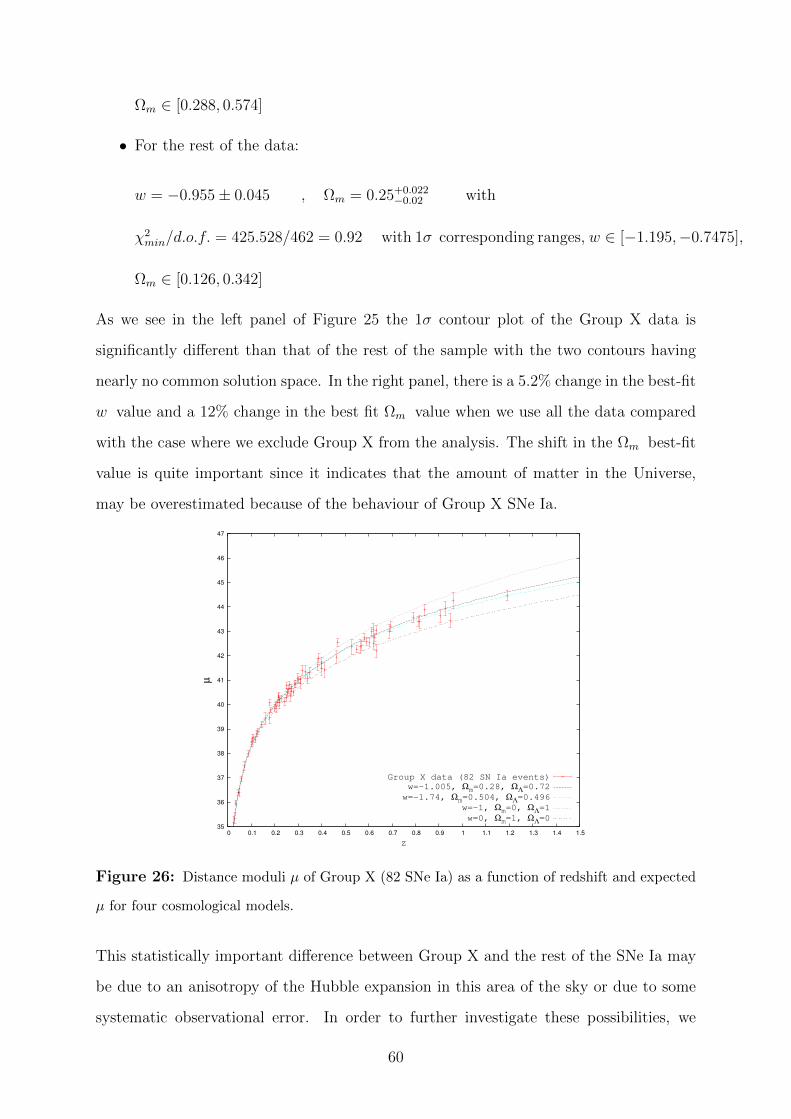
Ωm ∈ [0.288, 0.574]

• For the rest of the data:

w = −0.955± 0.045 , Ωm = 0.25+0.022−0.02 with

χ2min/d.o.f. = 425.528/462 = 0.92 with 1σ corresponding ranges, w ∈ [−1.195,−0.7475],

Ωm ∈ [0.126, 0.342]

As we see in the left panel of Figure 25 the 1σ contour plot of the Group X data is

significantly different than that of the rest of the sample with the two contours having

nearly no common solution space. In the right panel, there is a 5.2% change in the best-fit

w value and a 12% change in the best fit Ωm value when we use all the data compared

with the case where we exclude Group X from the analysis. The shift in the Ωm best-fit

value is quite important since it indicates that the amount of matter in the Universe,

may be overestimated because of the behaviour of Group X SNe Ia.

35

36

37

38

39

40

41

42

43

44

45

46

47

0 0.1 0.2 0.3 0.4 0.5 0.6 0.7 0.8 0.9 1 1.1 1.2 1.3 1.4 1.5

µ

z

Group X data (82 SN Ia events)

w=-1.005, Ωm=0.28, ΩΛ=0.72

w=-1.74, Ωm=0.504, ΩΛ=0.496

w=-1, Ωm=0, ΩΛ=1

w=0, Ωm=1, ΩΛ=0

Figure 26: Distance moduli µ of Group X (82 SNe Ia) as a function of redshift and expected

µ for four cosmological models.

This statistically important difference between Group X and the rest of the SNe Ia may

be due to an anisotropy of the Hubble expansion in this area of the sky or due to some

systematic observational error. In order to further investigate these possibilities, we

60

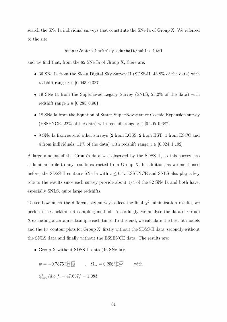
search the SNe Ia individual surveys that constitute the SNe Ia of Group X. We referred

to the site;

http://astro.berkeley.edu/bait/public html

and we find that, from the 82 SNe Ia of Group X, there are:

• 36 SNe Ia from the Sloan Digital Sky Survey II (SDSS-II, 43.8% of the data) with

redshift range z ∈ [0.043, 0.387]

• 19 SNe Ia from the Supernovae Legacy Survey (SNLS, 23.2% of the data) with

redshift range z ∈ [0.285, 0.961]

• 18 SNe Ia from the Equation of State: SupErNovae trace Cosmic Expansion survey

(ESSENCE, 22% of the data) with redshift range z ∈ [0.205, 0.687]

• 9 SNe Ia from several other surveys (2 from LOSS, 2 from HST, 1 from ESCC and

4 from individuals, 11% of the data) with redshift range z ∈ [0.024, 1.192]

A large amount of the Group’s data was observed by the SDSS-II, so this survey has

a dominant role to any results extracted from Group X. In addition, as we mentioned

before, the SDSS-II contains SNe Ia with z ≤ 0.4. ESSENCE and SNLS also play a key

role to the results since each survey provide about 1/4 of the 82 SNe Ia and both have,

especially SNLS, quite large redshifts.

To see how much the different sky surveys affect the final χ2 minimization results, we

perform the Jackknife Resampling method. Accordingly, we analyse the data of Group

X excluding a certain subsample each time. To this end, we calculate the best-fit models

and the 1σ contour plots for Group X, firstly without the SDSS-II data, secondly without

the SNLS data and finally without the ESSENCE data. The results are:

• Group X without SDSS-II data (46 SNe Ia):

w = −0.7875+0.1175−0.1225 , Ωm = 0.256+0.076

−0.07 with

χ2min/d.o.f. = 47.637/ = 1.083

61

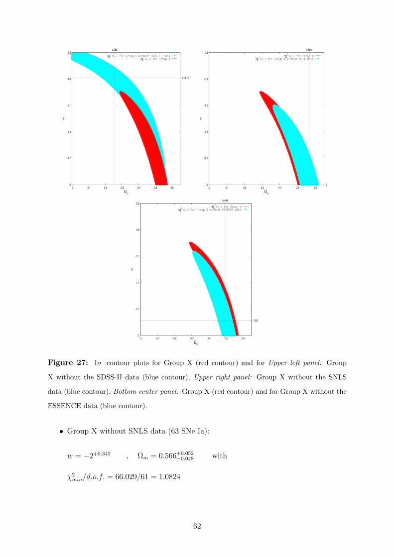
w

Ωm

∆χ2<2.3 for Group X without SDSS-II data

∆χ2<2.3 for Group X

-2

-1.7

-1.4

-1.1

-0.8

-0.5

0 0.1 0.2 0.3 0.4 0.5 0.6

-0.7875

0.256

w

Ωm

∆χ2<2.3 for Group X

∆χ2<2.3 for Group X without SNLS data

-2

-1.7

-1.4

-1.1

-0.8

-0.5

0 0.1 0.2 0.3 0.4 0.5 0.6

-2

0.566

w

Ωm

∆χ2<2.3 for Group X

∆χ2<2.3 for Group X without ESSENCE data

-2

-1.7

-1.4

-1.1

-0.8

-0.5

0 0.1 0.2 0.3 0.4 0.5 0.6

-1.83

0.496

Figure 27: 1σ contour plots for Group X (red contour) and for Upper left panel: Group

X without the SDSS-II data (blue contour), Upper right panel: Group X without the SNLS

data (blue contour), Bottom center panel: Group X (red contour) and for Group X without the

ESSENCE data (blue contour).

• Group X without SNLS data (63 SNe Ia):

w = −2+0.345 , Ωm = 0.566+0.052−0.048 with

χ2min/d.o.f. = 66.029/61 = 1.0824

62

• Group X without ESSENCE data (64 SNe Ia):

w = −1.83+0.2675−0.17 , Ωm = 0.496+0.042

−0.038 with

χ2min/d.o.f. = 76.767/62 = 1.238

The upper left panel of Figure 27 shows that excluding the SDSS-II data from the Group

X, we obtain a dramatic shift of the 1σ contour with respect to that of Group X unlike

the upper right and the bottom center panel, in which we have sequentially eliminated

the SNLS and the ESSENCE data respectively. Without the SDSS-II data, the ”banana-

shaped” 1σ contour shifts to a more consistent position with respect to that of the whole

SNe Ia. Moreover, excluding the SNLS or ESSENCE data, the SDSS-II subset becomes

more dominant in Group X, causing the 1σ contour to shift into even more negative values

of w and larger values of Ωm . The conclusion that can be drawn from Figure 27 and from

the above χ2min values is that this unusual behaviour of this sky region, is determined by

the SNe Ia of the SDSS-II survey. In other words, responsible for this difference in the

w -Ωm solution behaviour between the sky region of Group X and the rest of the sky are

the SDSS-II data in this region and not an actual anisotropy in the expansion. If there

was an anisotropy in Hubble flow for this sky region, it should probably be seen also at

all distant SNe Ia as well.

To see if there is a general systematic error in the SDSS-II survey, we compare the

solution results of many other SDSS-II SNe Ia from the sky region where the SDSS-

II focused from 2005 to 2007 (excluding Group X SNe Ia) as we mentioned in Section

3, with those of Group X. We remind the reader that this region is this characteristic

”smile” in the southern galactic hemisphere or, in equatorial coordinates, α ∈ [20h, 4h]

and δ ∈ [−1.25o, 1.25o]. We set an upper limit in redshift, 0.02 < z ≤ 0.4 since this is the

maximum redshift of SDSS-II data. Under these circumstances, 115 SNe Ia are left that

we can use within these coordinates and redshift limits. Obviously, SNe Ia from other

surveys can be included in these subsample but the vast majority of data comes from the

SDSS-II, allowing us to extract conclusions regarding a possible systematic behaviour of

the SDSS-II.

63

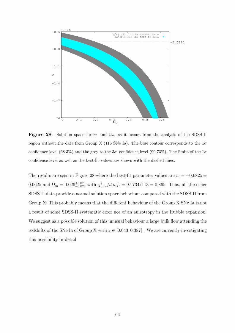
w

Ωm

∆χ2<11.83 for the SDSS-II data

∆χ2<2.3 for the SDSS-II data

-2

-1.7

-1.4

-1.1

-0.8

-0.5

0 0.1 0.2 0.3 0.4 0.5 0.6

-0.6825

0.026

Figure 28: Solution space for w and Ωm as it occurs from the analysis of the SDSS-II

region without the data from Group X (115 SNe Ia). The blue contour corresponds to the 1σ

confidence level (68.3%) and the grey to the 3σ confidence level (99.73%). The limits of the 1σ

confidence level as well as the best-fit values are shown with the dashed lines.

The results are seen in Figure 28 where the best-fit parameter values are w = −0.6825±

0.0625 and Ωm = 0.026+0.078−0.026 with χ2

min/d.o.f. = 97.734/113 = 0.865. Thus, all the other

SDSS-II data provide a normal solution space behaviour compared with the SDSS-II from

Group X. This probably means that the different behaviour of the Group X SNe Ia is not

a result of some SDSS-II systematic error nor of an anisotropy in the Hubble expansion.

We suggest as a possible solution of this unusual behaviour a large bulk flow attending the

redshifts of the SNe Ia of Group X with z ∈ [0.043, 0.387] . We are currently investigating

this possibility in detail

64

8 Conclusions

Several conclusions can be drawn based on the results of this thesis. First of all, high-z

SNe Ia are necessary in order to distinguish the QDE cosmological models. Observa-

tionally, there are sky regions with far more SNe Ia than others, mainly in the southern

galactic hemisphere. The best-fit cosmological parameters values with their 1σ uncertain-

ties for the Union2.1 sample, if we use the QDE cosmology model, are Ωm = 0.28+0.02−0.018,

w = −1.005±0.045 and q0 = −0.501±0.086, which is consistent with the other published

results and the ”concordance” cosmological model (Suzuki et al. 2012). We have searched

for possible anisotropies of the Hubble expansion, by dividing the sample into different

solid angles. We found no significant anisotropy in the Hubble expansion between the

two galactic hemispheres. However, we identified a particular sky region, with galactic

coordinates 35o < l < 83o & −79o < b < −37o, which provides a statistically significant

different w − Ωm solution with respect to the rest of the sample or any other subsample

that we have analysed. Although this could have been attributed to an anisotropy in

the Hubble flow, we found that this explanation is not supported by our analysis but

rather this result could well be due to a large bulk flow of galaxies at this region within

z ∼ 0.15− 0.3.

65

Appendices

A χ2 minimization, our data analysis method

The most common statistical method to see how well a theoretical model describes ob-

served data, is probably the χ2 (chi-squared) minimization procedure. Below we describe

the basics of this method which will be used throughout this thesis.

Suppose that we make a measurement (xi, yi) of a quantity y for a given xi. The expected

value for yi according to the theory would be f(xi) and the total error of the experimental

measurement (due to uncertainties of the measurement, etc.) would be σ. The probability

to make this measurement is 1

P (xi) =1

σi√

2πexp

[−1

2

(yi − f(xi)

σi

)2]

(A.1)

Now suppose that we make N measurements of this quantity that are independence of

each other. The total probability of obtaining this entire set of these N data points is

equal to the product of the probability of each data point (C. Laub, T. Kuhl), so

Ptot =N∏i=1

P (xi) =

[N∏i=1

1

σi√

2π

]exp

[−1

2

N∑i=1

(yi − f(xi)

σi

)2]

(A.2)

If we want to find the maximum probability we have to minimize the sum in the expo-

nential term of Ptot, so, we define this quantity as

χ2 =N∑i=1

(yi − f(xi)

σi

)2

(A.3)

and for χ2min we have the maximum probability. Thus, if the theoretical function f(xi,p),

depends on a set of parameters, which correspond to the elements of the vector p, we

can test for which values of these parameters we get the maximum probability.

1Probabilities are normalized to their maximum values (Plionis et al. 2011)

66

In our case, yi is the observed distance modulus of the each SN Ia, µobs(zi), which comes

with its redshift zi. Furthermore, f(xi) is the theoretical expected distance modulus

µth(zi,p) for the same redshift zi, with p ≡ (w,Ωm), for example. So, we have

χ2 =N∑i=1

(µobs(zi)− µth(zi,p)

σi

)2

(A.4)

with σi being the error in the distance modulus µi of each SN Ia. As we said before,

we have χ2min for the best-fitting parameters p0. When the parameters differ from these

values, p 6= p0, then χ2 increases, so ∆χ2 = χ2 − χ2min > 0. Limits of ∆χ2 that depend

on the number of the fitted parameters Nf , define confidence regions that contain a

certain fraction of the probability distribution of p’s 1. Almost every possibility region

corresponds to a certain standard deviation σ. All these are shown in Table 5.

Table 5: ∆χ2 limits for Nf fitted parameters and different confidence regions

σ P Nf = 1 Nf = 2 Nf = 3

1σ 68.3% 1 2.3 3.53

90% 2.71 4.61 6.25

2σ 95.4% 4 6.17 8.02

3σ 99.73% 9 11.83 14.2

In order to see how good our fit is, we have to divide the minimum χ2min by the degrees of

freedom, d.o.f. and get the reduced chi-square, χ2min/d.o.f. If we have N data points and

Nf fitted parameters, then d.o.f. = N −Nf . For a satisfactory fit we want χ2min/d.o.f. ≈

1. In other words, our model describes the observational data very well, inside our

uncertainties limits. If χ2min/d.o.f. 1 it means that our model is not an appropriate

fitting function or that we have not taken into account some form of unknown systematic

error. Finally, we may have underestimated our observational uncertainties (Bremer,

2009). On the other hand, if χ2min/d.o.f. 1, probably we have overestimated the

1For more information see ”Numerical Recipes 3rd Edition: The Art of Scientific Computing”, William

H. Press

67

statistical uncertainties and systematics. As a result, the 1σ possibility will cover a very

wide range of the fitted parameters, wide range of parameters, a non-desired effect.

B Joint likelihood analysis

In joint likelihood analysis, we take n fully independent data samples. For every combi-

nation of (w,Ωm) (we have a total of 195,000 combinations), we obtain a joint χ2 which

is given by

χ2 = χ21 + χ2

2 + · · ·+ χ2n (B.1)

while the degrees of freedom become

d.o.f. = d.o.f.1 + d.o.f.2 + · · ·+ d.o.f.n (B.2)

where (χ21 . . . χ

2n) are the values of χ2 for every one of the n independent data samples

while (d.o.f.1 . . . d.o.f.n) are the degrees of freedom of the χ2 analysis for every sample.

We then find the minimum, χ2min and the deviation of all the others from it, ∆χ2 =

χ2 − χ2min. Then, we plot the 1σ and 3σ contours (∆χ2 ≤ 2.3 and ∆χ2 ≤ 11.83

respectively) as they occur from the joint analysis.

68

9 References

Aguirre, A. N. 1999a, ApJ, 512, L19

Aguirre, A., & Haiman, Z. 2000, ApJ, 532, 28

Amanullah, R., et al. 2010, ApJ, 716, 712

Basset, B.A. & Hlozek, R. 2009, arxiv.org/abs/0910.5224

Betoule M. et al., 2014, ArXiv e-prints

Bianchi, S., Ferrara, A., 2006, MNRAS, 358, 379 ApJ, 596, L135

Corasaniti, P.S., 2006, MNRAS 372,191

Davies, J. I., Alton, P. B., Bianchi, S., Trewhella, M., 1998, MNRAS, 300, 1006

Davis, Mortsell, Sollerman and ESSENCE, 2007, astro-ph/0701510

Guy, J., et al. 2007, A&A, 466, 11

Hamuy, M., Phillips, M. M., Suntzeff, N. B., Schommer, R. A., Maza, J., & Aviles, R. 1996,

AJ, 112, 2391

Hicken, M., et al. 2009c, ApJ, 700, 1097

Kim, A.G., et al. 1997, ApJ, 476, L63

Kowalski, M., et al. 2008, ApJ, 686, 749

Laub, C. & Kuhl, T. A Critical Look at the Fitting of Reflectivity Models using the Reduced

Chi-Square Statistic. Retrieved from http://neutrons.ornl.gov

Menard, B., Kilbinger, M., & Scranton, R. 2010, MNRAS, 406, 1815

Perlmutter, S., et al. 1998, Nature, 391, 51

Perlmutter, S., et al. 1999, ApJ, 517, 565

Planck Collaboration 2014 A&A 571, A16

Plionis M., Terlevich R., Basilakos S., Bresolin F., Terlevich E., Melnick J., Chavez R., 2011,

MNRAS, 416, 2981

Riess, A. G., et al. 1998, AJ, 116, 1009

69

Riess, A. G., et al. 1999, AJ, 117, 707

Riess, A. G., et al. 2004, ApJ, 607, 665

Riess, A. G., et al. 2007, ApJ, 659, 98

Ryden, Barbara. Introduction to Cosmology. Ohio State Uni., 2003

Varvoglis, H & Seiradakis, J.H.,: Introduction to modern Astronomy, Thessaloniki: Gargatanis

, 1994

Shustov, B. M., Vibe, D. Z., 1995, Astronomy Reports, 39, 579

Sullivan, M., et al. 2003, MNRAS, 340, 1057

Sullivan, M., et al. 2006, ApJ, 648, 868

Sullivan, M., et al. 2010, MNRAS, 406, 782

Suzuki N. et al., 2012, ApJ, 746, 85

Wu, P., Zhengxiang, L. & Hongwei, Y., 2015, arXiv:1501.01818

Yoon, S.C. & Langer, N., 2004, Astron.Astrophys.435:967-985,2005

70