Embed Size (px)
Citation preview
CONSTRAINING MASSIVE BLACK HOLE POPULATION MODELS WITH
GRAVITATIONAL WAVE OBSERVATIONS
by
Joseph Eugene Plowman
A dissertation submitted in partial fulfillmentof the requirements for the degree
of
Doctor of Philosophy
in
Physics
MONTANA STATE UNIVERSITYBozeman, Montana
May, 2010

c© Copyright
by
Joseph Eugene Plowman
2010
All Rights Reserved
ii
APPROVAL
of a dissertation submitted by
Joseph Eugene Plowman
This dissertation has been read by each member of the dissertation committee andhas been found to be satisfactory regarding content, English usage, format, citations,bibliographic style, and consistency, and is ready for submission to the Division ofGraduate Education.
Dr. Ronald W. Hellings
Approved for the Department of Physics
Dr. Richard Smith
Approved for the Division of Graduate Education
Dr. Carl A. Fox
iii
STATEMENT OF PERMISSION TO USE
In presenting this dissertation in partial fulfillment of the requirements for a doc-
toral degree at Montana State University, I agree that the Library shall make it
available to borrowers under rules of the Library. I further agree that copying of this
dissertation is allowable only for scholarly purposes, consistent with “fair use” as pre-
scribed in the U.S. Copyright Law. Requests for extensive copying or reproduction of
this dissertation should be referred to ProQuest Information and Learning, 300 North
Zeeb Road, Ann Arbor, Michigan 48106, to whom I have granted “the non-exclusive
right to reproduce and distribute my dissertation in and from microform along with
the non-exclusive right to reproduce and distribute my abstract in any format in
whole or in part.”
Joseph Eugene Plowman
May, 2010
iv
DEDICATION
To my parents, for years of love and support
In memory of William Hiscock
v
ACKNOWLEDGEMENTS
This dissertation makes use of black hole population model results kindly provided
by Dr. Marta Volonteri, which have significantly enhanced the relevance of this work.
I am indebted to Dr. Volonteri for allowing me to use these results.
The parameter estimation errors used in this dissertation were calculated using
the LISA calculator, provided by Dr. Jeff Crowder, and the Montana/MIT group
spinning black hole code, provided by Drs. Scott Hughes and Neil Cornish.
The research presented in this dissertation was supported in part by grants and
fellowships from Montana NASA EPSCoR and the Montana NASA Space Grant
Consortium, which have been indispensable in allowing me to concentrate on the
research and complete it in a timely fashion.
I also gratefully acknowledge support from the William Hiscock Memorial Schol-
arship during my final Spring semester.
Each of my committee members have been instrumental in bringing this work to
fruition, in particular my advisor, Dr. Ron Hellings, and Dr. Charles Kankelborg,
with whom I have had many fruitful discussions.
Portions of this work were carried out with additional assistance from Daniel
Jacobs, Ron Hellings, Shane Larson, and Sachiko Tsuruta.
vi
TABLE OF CONTENTS
1. INTRODUCTION ........................................................................................1
2. MASSIVE BLACK HOLES: BACKGROUND ................................................4
2.1 Existence of Supermassive Black Holes ......................................................42.2 SMBH Origins .........................................................................................42.3 Modeling the MBH Merger and Accretion History......................................62.4 Generation of Halo Merger Histories..........................................................72.5 The Black Hole Seed Population ...............................................................92.6 Merger and Accretion Processes .............................................................. 102.7 MBH Observation Prospects ................................................................... 13
3. GRAVITATIONAL WAVES ........................................................................ 16
3.1 Overview ............................................................................................... 163.2 Production of Gravitational Waves.......................................................... 203.3 Detection of Gravitational Waves ............................................................ 253.4 LISA Detection...................................................................................... 303.5 BBH Parameters & their Errors .............................................................. 34
4. MODEL COMPARISON............................................................................. 41
4.1 The 1-D K-S Test and Variants............................................................... 424.2 Two-Dimensional Tests .......................................................................... 474.3 Validation of Tests ................................................................................. 51
5. CONSTRAINING MBH POPULATIONS USING THE ERROR KERNEL.... 63
5.1 Calculating the Error Kernel .................................................................. 635.1.1 Applying the Error Kernel............................................................... 68
5.2 Discriminating Between Population Models ............................................. 715.2.1 Convolving The Models with the LISA Error Kernel ......................... 715.2.2 Discriminating Between Models ....................................................... 72
6. DIRECT APPLICATION OF ERRORS; 2-DIMENSIONAL TESTS.............. 77
6.1 Direct Error Application Method ............................................................ 826.2 The Parameter Estimation Errors & Estimated Parameter Distributions ... 856.3 Model Comparison Results; 1 and 2 Dimensions....................................... 91
6.3.1 Effects of Parameter Estimation Errors on Model Distinguishability. 1006.4 Summary............................................................................................. 101

vii
TABLE OF CONTENTS – CONTINUED
7. CONCLUSION......................................................................................... 105
8. FUTURE WORK ..................................................................................... 108
REFERENCES CITED.................................................................................. 109
viii
LIST OF TABLESTable Page
3.1 The parameters which define a source. There are a variety of combi-nations of m1 and m2 which can be used to specify the masses of thesource, depending on context ............................................................... 39
5.1 This table of parameters lists the completely marginalised case param-eters (grey boxes) along with their ranges and describes the treatmentof the three population parameters. Reduced mass ratio η is averaged,z is held constant and total mass (Mtot) is divided into three units. ....... 66
5.2 Comparisons of models before and after convolution with LISA kernel,for binaries coalescing within the observation window, assuming oneyear of observation time. The ‘Before LISA’ comparisons effectivelyassume that all of the sources are detectable and have zero redshifterror, while the ‘After LISA’ comparisons incorporates the effects ofboth parameter uncertainty and detectability. E is the maximum devi-ation between the cumulative histograms of random draws from the twomodels. Q is the corresponding probability that random fluctuationscould be responsible for the deviation. .................................................. 76
6.1 The Press-Schechter weights, fiducial masses, and numbers of trees forthe model results compared in this chapter. .......................................... 79
6.2 Third quartiles (75th percentiles) of the standard deviation of esti-mated parameters for each of the four models considered. ...................... 88
6.3 E statistic Model comparison results for 1 year of observation, showingthe fraction of confidence levels which were above 95%. To make thetable easier to read, comparisons where 1/2 of the confidence levelswere above 95% are marked in light gray, comparisons where 3/4 wereabove 95% are marked in medium gray, and those where 9/10 wereabove 95% are marked in dark gray. ..................................................... 96
ix
LIST OF TABLES – CONTINUEDTable Page
6.4 E statistic Model comparison results for 3 years of observation, showingthe fraction of confidence levels which were above 95%. To make thetable easier to read, comparisons where 1/2 of the confidence levelswere above 95% are marked in light gray, comparisons where 3/4 wereabove 95% are marked in medium gray, and those where 9/10 wereabove 95% are marked in dark gray. ..................................................... 97
6.5 E statistic Model comparison results for 5 years of observation, showingthe fraction of confidence levels which were above 95%. To make thetable easier to read, comparisons where 1/2 of the confidence levelswere above 95% are marked in light gray, comparisons where 3/4 wereabove 95% are marked in medium gray, and those where 9/10 wereabove 95% are marked in dark gray. ..................................................... 97
6.6 E statistic Model comparison results for 1 year of observation with noparameter estimation errors, showing the fraction of confidence levelswhich were above 95%. To make the table easier to read, comparisonswhere 1/2 of the confidence levels were above 95% are marked in lightgray, comparisons where 3/4 were above 95% are marked in mediumgray, and those where 9/10 were above 95% are marked in dark gray. ... 102
6.7 The difference between the fraction of confidence levels which wereabove 95% without parameter estimation errors and with parameter es-timation errors. To make the table easier to read, differences above 0.1are marked in light gray, differences above 0.2 are marked in mediumgray, and those above 0.3 are marked in dark gray. .............................. 102
x
LIST OF FIGURESFigure Page
3.1 Diagram showing the configuration of the LIGO instrument................... 18
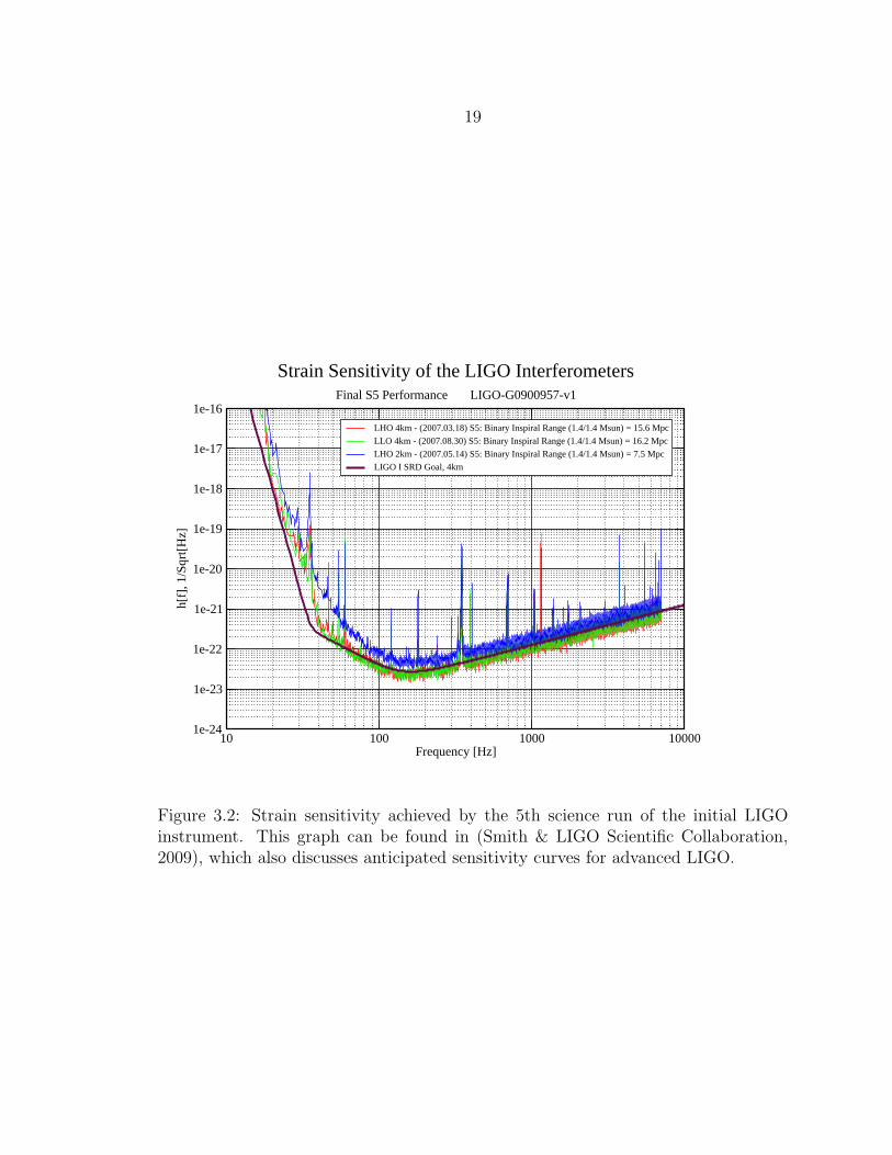
3.2 Strain sensitivity achieved by the 5th science run of the initial LIGOinstrument. This graph can be found in (Smith & LIGO Scientific Col-laboration, 2009), which also discusses anticipated sensitivity curves foradvanced LIGO. .................................................................................. 19
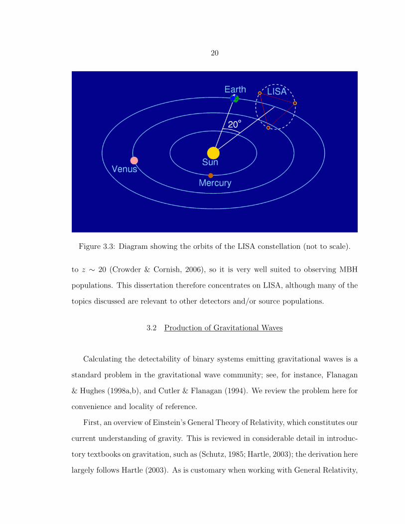
3.3 Diagram showing the orbits of the LISA constellation (not to scale). ...... 20
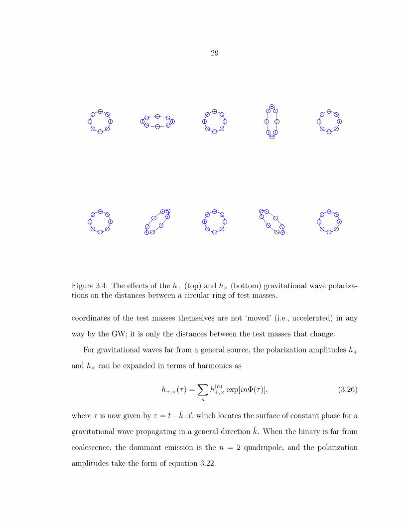
3.4 The effects of the h+ (top) and h× (bottom) gravitational wave polar-izations on the distances between a circular ring of test masses. ............. 29
3.5 Example spinning binary waveform. The binary mass ratio ism1/m2 =10 and the (redshifted)Mc = 106. The spin of the more massive binarybegins aligned with the orbit, while the spin of the smaller binary isrotated by 40 with respect to the orbit. The waveform has a Hannwindow applied to the final orbits, to reduce ringing in the Fourier domain.36
3.6 Example plot showing the difference between parameter distributionsexpressed in terms of redshifted (top) and non-redshifted (bottom)mass variables. Note that an SNR cut has been applied to these dis-tributions............................................................................................ 38
4.1 Example Probability Density Function (PDF) and Cumulative Dis-tribution Function (CDF), for the χ2 statistic. The PDF indicatesthe fraction of draws from the distribution which fall between χ2 andχ2 + dχ2, while the CDF is the fraction of draws which are less thanχ2. The CDF is thus the integral of the PDF. ....................................... 43
4.2 Comparison of two example data sets illustrating the calculation ofthe E statistic. Top plots show the two cumulative histograms usedin calculating the E statistic, as well as the differences between them.The lower left plot shows only the differences between the two pairs ofhistograms, the largest of which is the E statistic. Shown in the lowerright are the normalized cumulative distribution functions on whichthe K-S test is based. These example data sets were created with theprobability density function (PDF) p(x) = xα/(1 +α) (x ranging fromzero to one), and Poisson distributed total number counts. Data set Ahad α = 0.6 and Poisson parameter 56, while data set B had 1.5 and 72 . 45
xi
LIST OF FIGURES – CONTINUEDFigure Page
4.3 Cumulative distribution function of one-dimensional E statistics, for2.5×105 draws given the null hypothesis. For each draw, two simulateddata sets were produced, each with total number of data points drawnfrom a Poisson distribution with λ = 25000 and individual data pointsdrawn from a uniform distribution over 0 . . . 1. The E statistics result-ing from these draws were then tabulated into a cumulative histogramand normalized, resulting in this plot. Shown for comparison is theequivalent CDF of the differences between the number counts, |NA−NB|.48
4.4 Example confidence levels for the K-S test (left), the E statistic (right),and the statistic formed by taking the difference between the totalnumber counts (a χ2 statistic with only one degree of freedom). Datasets were produced in the same way as in Figure 4.2.............................. 49
4.5 Cumulative Distribution Functions for two-dimensional E statistics,each made using 5 × 10⁴ draws given the null hypothesis. Calculatedin a similar fashion to that described in the caption of Figure 4.3 ........... 51
4.6 Histogram of a Lorentzian Distribution. Draws falling outside of thedesignated histogram range have been placed into the outermost bins,illustrating the large tails of the distribution ......................................... 54
4.7 Histogram of confidence levels comparing data sets drawn given thenull hypothesis. Individual data points were Lorentzian distributed,and number counts varied according to a Poisson distribution. Poissonrate parameter and Lorentzian median and HWHM parameters variedrandomly from one comparison to the next, as discussed in the text ....... 55
4.8 Two dimensional test distribution consisting of a completely correlatedGaussian distribution along the line defined by θ = 45 .......................... 56
4.9 Two dimensional test distribution consisting of two overlapping, elon-gated, rotated 2-dimensional Gaussians................................................. 57
4.10 Two dimensional test distribution consisting of a single circular twodimensional Gaussian distribution (see Figure 4.10 ................................ 58
xii
LIST OF FIGURES – CONTINUEDFigure Page
4.11 Cumulative histogram of confidence levels for draws given the null hy-pothesis with semi-correlated distributions. Also shown is the straightline of unit slope which is the correct cumulative histogram in thelimit of a large number of draws and a large number of samples ineach draw. 5000 draws were made given the null hypothesis, with eachdata set having a Poisson total number count with parameter λ = 200.Individual data points were drawn from the same distribution as thatshown in Figure 4.9 ............................................................................. 59
4.12 Cumulative histogram of confidence levels for draws given the null hy-pothesis with fully correlated distributions. Also shown is the straightline of unit slope which is the correct cumulative histogram in thelimit of a large number of draws and a large number of samples ineach draw. 5000 draws were made given the null hypothesis, with eachdata set having a Poisson total number count with parameter λ = 200.Individual data points were drawn from the same distribution as thatshown in Figure 4.8 ............................................................................. 60
4.13 Cumulative histogram of confidence levels for null hypothesis drawswith uncorrelated distributions. Also shown is the straight line of unitslope which is the correct cumulative histogram in the limit of a largenumber of draws and a large number of samples in each draw. 5000draws were made given the null hypothesis, with each data set havinga Poisson total number count with parameter λ = 200. Individual datapoints were drawn from the same distribution as that shown in Figure4.10 .................................................................................................... 61
xiii
LIST OF FIGURES – CONTINUEDFigure Page
5.1 Creating the error kernel for the ‘medium mass’ bin and marginalisedparameters described in Table 5.1, total masses between 10, 000Mand 100, 000M. a) The Gaussian PDF implied by simple RMS er-ror. b) Adding the probability densities resulting from many differentmarginalised parameters results in a highly non-normal distribution.Shown here (in solid black) is the distribution of possible detectionsgiven several hundred sources at a redshift of 10 in a mass range104 : 106M. Overlaid (in dashes) is the distribution obtained bysimply adding the errors in quadrature. c) The zs = 10 PDF insertedinto its place in the error kernel. Source redshifts are sampled at evenredshift intervals of 0.25. d) 70% confidence intervals for LISA de-termination of redshift gives an overview of the resulting error kernel........................................................................................................... 69
5.2 Average fractional error for binaries with total mass between 10, 000Mand 1, 000, 000M and reduced mass between 0.001 and 0.25, using +for redshift and x for reduced mass. Chirp mass errors are not shown,but are an order of magnitude below the reduced mass errors. Error inredshift dominates the reduced mass error by over an order of magnitude.70
5.3 The effect of the LISA error kernel on the MBH binary populationpredicted by Volonteri et al. (2003) for a 3 year observation. Solid line:modelled source distribution for masses below 108M. Dotted line:modelled source distribution with SNR > 8 cut, as applied by Sesanaet al. (2007). Dashed line: convolution of modelled source distributionwith LISA error kernel. The error kernel distribution incorporates thelarge errors inherent to binary redshift determination. ........................... 73
5.4 Binary merger redshift spectra, after smearing by the LISA error kernelin the style of Sesana et al. (2007). Solid line - VHM, short-long dashedline - KBD, short dashed line - BVRlf, dashed line - BVRhf................... 74
6.1 The source parameter distribution of m1 (the redshifted mass of thelarger black hole) for binaries detected by LISA. An SNR cutoff hasbeen applied (SNR = 10) to the model distribution, but no parameterestimation uncertainties. ...................................................................... 80
xiv
LIST OF FIGURES – CONTINUEDFigure Page
6.2 The source parameter distribution of m2 (the redshifted mass of thesmaller black hole) for binaries detected by LISA. An SNR cutoff hasbeen applied (SNR = 10) to the model distribution, but no parameterestimation uncertainties. ...................................................................... 80
6.3 The source parameter distribution of DL for binaries detected by LISA.An SNR cutoff has been applied (SNR = 10) to the model distribution,but no parameter estimation uncertainties. ........................................... 81
6.4 The source parameter distribution of the spin of the larger black holefor binaries detected by LISA. An SNR cutoff has been applied (SNR =10) to the model distribution, but no parameter estimation uncertainties.81
6.5 The source parameter distribution of the spin of the smaller black holefor binaries detected by LISA. An SNR cutoff has been applied (SNR =10) to the model distribution, but no parameter estimation uncertainties.82
6.6 Quartiles of the luminosity distance estimation errors for the SC (smallseeds, small spins) model. This figure illustrates the lack of dependenceof the error on tc, and as a result we only use error distributions pro-duced with a one year range of tc, even for longer observation windows... 83
6.7 The effects of parameter estimation errors on some example distri-butions. The original source parameter distributions are shown withunfilled heavy lines, while the estimated parameter distributions (in-corporating errors) are shown as a filled histogram with light lines.In every case, the error distributions are Gaussians with unit variance.The errors have a significant effect on Example B, but not on ExamplesA and C. ............................................................................................ 86
6.8 The parameter estimation error in lnm1 (the redshifted mass of thelarger black hole) for binaries detected by LISA. ................................... 88
6.9 The parameter estimation error in lnm2 (the redshifted mass of thesmaller black hole) for binaries detected by LISA. ................................. 89
xv
LIST OF FIGURES – CONTINUEDFigure Page
6.10 The parameter estimation error in lnDL for binaries detected by LISA. .. 89
6.11 The parameter estimation error in the spin of the larger black hole forbinaries detected by LISA. ................................................................... 90
6.12 The parameter estimation error in the spin of the smaller black holefor binaries detected by LISA. .............................................................. 90
6.13 The estimated parameter distribution of m1 (the redshifted mass ofthe larger black hole) for binaries detected by LISA. Also shows thecorresponding source parameter distribution (an SNR=10 cutoff hasbeen applied to both distributions). ...................................................... 92
6.14 The source parameter distribution of m2 (the redshifted mass of thesmaller black hole) for binaries detected by LISA. Also shows the cor-responding source parameter distribution (an SNR=10 cutoff has beenapplied to both distributions)............................................................... 92
6.15 The source parameter distribution of DL for binaries detected byLISA. Also shows the corresponding source parameter distribution (anSNR=10 cutoff has been applied to both distributions).......................... 93
6.16 The source parameter distribution of the spin of the larger black holefor binaries detected by LISA. Also shows the corresponding sourceparameter distribution (an SNR=10 cutoff has been applied to bothdistributions). ..................................................................................... 93
6.17 The source parameter distribution of the spin of the smaller black holefor binaries detected by LISA. Also shows the corresponding sourceparameter distribution (an SNR=10 cutoff has been applied to bothdistributions). ..................................................................................... 94
6.18 Distributions of estimated m1 and DL parameters. With 3 years ofsources, the SC and SE models cannot consistently be distinguished,while the LE and LC models can often (in 77% of realizations) bedistinguished at 95% confidence. Other 3 year comparisons consistentlygive 95% or greater confidence levels..................................................... 98
xvi
LIST OF FIGURES – CONTINUEDFigure Page
6.19 Distributions of estimated m2 and DL parameters. With 3 years ofsources, the SC and SE models cannot consistently be distinguished,while the LE and LC models can sometimes (in 59% of realizations) bedistinguished at 95% confidence. Other 3 year comparisons consistentlygive 95% or greater confidence levels..................................................... 99
xvii
ABSTRACT
A number of scenarios have been proposed for the origin of the supermassive blackholes (SMBHs) that are found in the centres of most galaxies. Many such scenariospredict a high-redshift population of massive black holes (MBHs), with masses in therange 102 to 105 times that of the Sun. When the Laser Interferometer Space Antenna(LISA) is finally operational, it is likely that it will detect on the order of 100 of theseMBH binaries as they merge. The differences between proposed population modelsproduce appreciable effects in the portion of the population which is detectable byLISA, so it is likely that the LISA observations will allow us to place constraints onthem. However, gravitational wave detectors such as LISA will not be able to detectall such mergers nor assign precise black hole parameters to the merger, due to weakgravitational wave signal strengths. This dissertation explores LISA’s ability to distin-guish between several MBH population models. In this way, we go beyond predictinga LISA observed population and consider the extent to which LISA observationscould inform astrophysical modelers. The errors in LISA parameter estimation areapplied in two ways, with an ‘Error Kernel’ that is marginalized over astrophysicallyuninteresting ‘sample’ parameters, and with a more direct method which generatesrandom sample parameters for each source in a population realization. We considerhow the distinguishability varies depending on the choice of source parameters (1 or2 parameters chosen from masses, redshift or spins) used to characterize the modeldistributions, with confidence levels determined by 1 or 2-dimensional tests based onthe Kolmogorov-Smirnov test.
1
CHAPTER 1
INTRODUCTION
There is substantial evidence (e.g., Kormendy & Richstone, 1995; Richstone et al.,
1998) for the existence of supermassive black holes (SMBHs) in the nuclei of most
galaxies, the black hole in our own galaxy being the best studied and most clearly
justified of these objects. However, the origin of these black holes remains an unsettled
question. In one scenario, the more massive black holes formed from the merger and
coalescence of smaller ‘seed’ black holes created in the very early Universe (e.g., Madau
& Rees, 2001). Several models of this process have been proposed and numerically
simulated (e.g., Haehnelt & Kauffmann, 2000; Volonteri et al., 2003). Typical seed
black holes have masses M• ∼ 100M at high redshift (e.g., z ∼ 20), so these models
predict an evolving population of massive black holes (MBHs), with masses that can
cover the entire range from ∼ 100 to 109M.
Younger members of this population fall into the intermediate-mass range (100M
. . . 105M), and are not suited to electromagnetic detection, making it very difficult
to verify a particular formation and evolution scenario or to discriminate between
models. When the Laser Interferometer Space Antenna (LISA) is finally operational,
however, it is likely that it will detect on the order of 100 merging MBH Binaries in
the range Mtot & 1000M. Since the differences between proposed population models
produce appreciable effects in the subset of the population that LISA can detect,
LISA observations should allow us to place constraints on the models.
Once we have the LISA detected population in hand, we will need to determine
how it constrains models of the astrophysical population which gave rise to it. Equiv-
alently, we will want to know which model (with its associated parameters) is most
likely to have produced the observed population. We also want to know how strongly
2
the LISA data set will constrain the models: How dissimilar from the actual popu-
lation does a model population need to be before it can be distinguished based on
the LISA data? Fully answering this question requires considering LISA’s ability to
detect sources, the parameter estimation errors associated with sources inferred from
the LISA data, and, eventually, the a posteriori source parameter distributions of
sources extracted from the LISA data. It also requires considering how to quantify
the differences between populations as they would be observed from the LISA data
and associating a degree of confidence with these difference quantities.
In this dissertation, we consider methods of applying the parameter estimation
errors and LISA detection thresholds, apply these methods to various population
models, and compare the resulting distributions of estimated parameters using varia-
tions of the Kolmogorov-Smirnov (K-S) test. We consider how the distinguishability
of the models depends on a variety of factors (see below). The results demonstrate
the ability of LISA to constrain the astrophysics of MBH formation, and shed light
on the directions of future research in MBH population models, LISA instrument
models, and model comparison efforts.
The organization of this dissertation is as follows. Chapter 2 reviews the astro-
physical models of MBH formation and evolution. Chapter 3 gives overviews of the
production of Gravitational Waves (GWs), their effects and detection with LISA, and
calculation of LISA parameter estimation errors using the Fisher Information Matrix
approximation. It also describes the LISA instrument and lists the parameters which
determine the GW signal, highlighting the ‘population’ parameters which are rele-
vant to the astrophysical population models. In Chapter 4, we describe the statistical
tests we use to assess the distinguishability between models. In particular, we define a
modified version of the K-S test which is sensitive to the differences between the model
predictions of overall number count in addition to differences between the individual
3
source parameter distributions (the standard K-S test is only sensitive to the latter).
Chapter 5 describes an ‘error kernel’, K(λi, λi), that marginalizes the LISA parameter
estimation errors over the MBH binary parameters (‘sample’ parameters) which have
the same distributions for all models. We apply this error kernel to several model
results obtained from the literature, producing estimated detection rates as functions
of the best-fit parameter values and comparing the resulting distributions. In Chapter
6, we apply the LISA parameter estimation errors to four sets of simulation results
obtained from Dr. Marta Volonteri, generating random sample parameters for each
source appearing in the simulation results. We compare the resulting distributions
of parameters between each of the models, investigating how their distinguishability
depends on the LISA observation time, which BH parameters are compared, and
whether or not the parameter estimation errors are applied to the model parameter
distribution. Chapter 7 draws conclusions from this work and indicates the direction
for future research on this topic.
4
CHAPTER 2
MASSIVE BLACK HOLES: BACKGROUND
2.1 Existence of Supermassive Black Holes
Observations of the high redshift quasar population (Fan et al., 2001; Stern et al.,
2000; Zheng et al., 2000; Becker et al., 2001) suggest that a population of SMBHs has
existed since early epochs (z ∼ 6). The local census of SMBHs has been increasing in
recent years (Tremaine et al., 2002), driven by a growing body of observational evi-
dence linking the mass of SMBHs with observational properties of their host galaxies.
Early studies revealed a rough correlation between SMBH mass and the bulge lumi-
nosity of the host galaxy (Kormendy & Richstone, 1995; Magorrian et al., 1998). A
much stronger correlation was later discovered between the SMBH mass, M•, and the
stellar velocity dispersion, σ, in the galactic core, the so-called ‘M -σ’ relation (Geb-
hardt et al., 2000; Ferrarese & Merritt, 2000; Tremaine et al., 2002). The current best
fit to the M -σ relation (Merritt & Ferrarese, 2001; Tremaine et al., 2002) gives the
mass of the central black hole M• as
log
(M•
M
)= 8.13 + 4.02 log
(σ
200km/s
). (2.1)
The observational data supporting the M − σ relation currently spans a mass range
from ∼ 105M to ∼ 109M.
2.2 SMBH Origins
Given this observational evidence for the existence of an SMBH population, the
question arises: how did these objects come to be? What is the nature of the initial
5
population? Several SMBH progenitor scenarios are proposed (see Volonteri et al.,
2003; Portegies Zwart et al., 2004a; Begelman et al., 2006; Mack et al., 2007):
1. Direct gravitational core collapse of pregalactic dark halos,
2. Growth from smaller seed black holes through merging and accretion over time,
3. Gravitational runaway collapse of dense star clusters,
4. Primordial BH remnants from the big bang.
In case 1, SMBHs can form very early in the Universe through direct collapse of dark
matter halo with mass of ∼ 106M or larger (Bromm & Loeb, 2003), or from direct
core collapse of mini halos through a quasi-star phase instead of through ordinary
stellar evolution (Begelman et al., 2006), leading to a population with masses in the
range ∼ 104M to ∼ 106M. In case 2, on the other hand, (Madau & Rees, 2001;
Haehnelt & Kauffmann, 2000; Volonteri et al., 2003; Tanaka & Haiman, 2009), seed
black holes produced in the early universe can be significantly smaller and grow by
accretion, coalescences and merging, leading to the population of SMBHs seen in the
Universe today. In most cases (e.g., Volonteri et al., 2003), the seed black holes have
mass less than ∼ 300M and are the remnants of Population III stars. Detailed stellar
evolution calculations have recently found, however, that these seed black holes can
be remnants of very massive Population III stars, referred to as CVMSs (Tsuruta
et al., 2007; Ohkubo et al., 2009; Umeda et al., 2009). These metal-free CVMSs
evolve quickly and then collapse in the early universe, yielding an IMBH population
with masses in the range of ∼ 500M − 10, 000M.
The scenario involving direct collapse is not difficult to distinguish from that
involving Population III stars, because the former predicts only a small number of
the more massive BHs while the latter predicts considerably more BHs with a wider
6
range of masses and redshifts. In case 3 (e.g., Ebisuzaki et al., 2001; Portegies Zwart
et al., 2004b,c), IMBHs (of ∼ 1000M) can be formed at any time in dense star
clusters and grow by merging in the given environment. Such a process can produce
a low level population of mergers at all redshifts. Although there is currently no
evidence for the existence of primordial BHs, case 4 is theoretically possible (Mack
et al., 2007). In each case, these seed populations can grow through merger and
accretion into the population of SMBHs observed today. This dissertation considers
population model results produced with the high mass Begelman et al. (2006) and
low mass Volonteri et al. (2003) seed populations.
2.3 Modeling the MBH Merger and Accretion History
Models of SMBH evolution through merging and accretion generally make use of a
‘merger-tree’ framework(Volonteri et al., 2003; Cole et al., 2000). In these frameworks,
generation of the MBH merger and accretion history proceeds in three stages:
• First, the history of the parent dark matter haloes is constructed, often starting
with our understanding of the present-day distribution of haloes and working
backwards to high redshift.
• The high-redshift progenitor haloes are seeded with massive black hole progen-
itors based on the seed population model (e.g., BVR’s high-mass seeds, etc).
• The already-generated halo merger history is then followed forward in time,
applying our understanding of merging and accretion processes to the MBHs to
evolve them along with their parent haloes.
Each aspect of this process can be carried out in various ways; we review some of
them below.
7
2.4 Generation of Halo Merger Histories
The history of the dark matter haloes is carried out first. As dark matter com-
poses over 80% of the mass of the universe (Jarosik et al., 2010) and interacts only
gravitationally with other matter, its evolution is largely independent of the baryonic
components. The baryonic components (in this case, the SMBH progenitors), on the
other hand, are gravitationally bound to the dark matter haloes, and follow their
merger history.
The dark matter halo history can be evaluated either directly using numerical
N-body simulations (e.g., Micic et al., 2007), or via a hybrid Monte Carlo technique
using an analytical halo merger probability. This section concentrates on the semi-
analytical techniques, since the models used in this dissertation are based on such
techniques. The discussion is based on Cole et al. (2000), Volonteri et al. (2003), and
Somerville & Kolatt (1999).
These models have their origins in the work of Press & Schechter (1974), which
envisioned a process of self-similar condensation growing out of statistical randomness
in an “incoherent dust” model:
“As the expanding Friedmann cosmology evolves, the mass points con-
dense into aggregates which (when they are themselves sufficiently bound),
we identify as single particles of a larger mass. In this way, the condensa-
tion proceeds to larger scales.
. . .
When condensation has proceeded to lumpiness on a certain scale, the
statistical randomness in the positions of the discrete lumps is itself a
perturbation to all larger scales, and this causes condensation of increas-
8
ingly large masses at later and later times. We take these statistical
fluctuations as the only source of long-wavelength perturbations.”
They were able to use this description to calculate the number density of haloes as a
function of their mass and redshift, and the results agree with the results of N-body
simulations (Efstathiou et al., 1988).
The Press-Schechter model has since been extended (Lacey & Cole, 1993a; Bond
et al., 1991) to calculate the conditional probability that a halo at some mass and
redshift had a progenitor at some earlier redshift in a specified mass range. The
results of these models also agree with N-body simulations (Lacey & Cole, 1994).
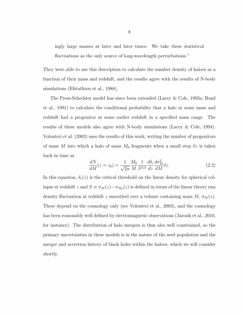
Volonteri et al. (2003) uses the results of this work, writing the number of progenitors
of mass M into which a halo of mass M0 fragments when a small step δz is taken
back in time as
dN
dM(z = z0) =
1√2π
M0
M
1
S3/2
dδcdz
dσ2M
dMδz. (2.2)
In this equation, δc(z) is the critical threshold on the linear density for spherical col-
lapse at redshift z and S ≡ σM(z)−σM0(z) is defined in terms of the linear theory rms
density fluctuation at redshift z smoothed over a volume containing mass M , σM(z).
These depend on the cosmology only (see Volonteri et al., 2003), and the cosmology
has been reasonably well defined by electromagnetic observations (Jarosik et al., 2010,
for instance). The distribution of halo mergers is thus also well constrained, so the
primary uncertainties in these models is in the nature of the seed population and the
merger and accretion history of black holes within the haloes, which we will consider
shortly.
9
The semi-analytic halo merger model then proceeds by recursive application of
Equation 2.2 to modern-day haloes at various fiducial masses1, repeatedly breaking
the haloes up into progenitors at increasingly high redshift and tracking the resulting
hierarchy of mergers. The process is repeated multiple times to ensure that the
statistical variation in the merger tree has been adequately sampled.
2.5 The Black Hole Seed Population
After the halo merger tree has been determined, the high-redshift haloes are seeded
with progenitor black holes that will grow by merger and accretion into modern-day
SMBHs. There are multiple unknowns in this seed population, including:
• The mass distribution of the seeds. These can range from ∼ 100M in some
models to ∼ 105M in others.
• The redshift at which they occur, typically between z = 10 and z = 20.
• The frequency with which they occur; usually only a small fraction of the high-
redshift haloes host a progenitor BH.
In one common scenario (Madau & Rees, 2001; Volonteri et al., 2003), the seeds
are the remnants of massive Population III stars, with masses in the hundreds of
M (according to Volonteri et al., 2003, the precise mass used makes little difference
to the simulation results). They occur at z ∼ 20 and are placed in only the most
massive haloes, those whose density exceeds the mean by some threshold (e.g. 3.5σ).
This corresponds to mini-haloes of mass ∼ 107M in a standard ΛCDM cosmology,
1To relate the results to the population in the universe, each fiducial mass has a corresponding
weighting which is determined by observations of the modern-day universe.
10
and seeded haloes account for ∼ 0.0005 of the total halo mass (given a Gaussian
distribution).
Another scenario which has received considerable attention of late is that of Begel-
man et al. (2006). They suggest that BHs of mass & 105M can be formed prior to
z ∼ 10 in haloes with low angular momentum and viral temperatures & 104K. There,
global dynamical instabilities such as the ‘bars-within-bars’ mechanism (Shlosman
et al., 1989) can lead to the formation of a ‘quasi-star’ with ∼ 105M. The quasi-star
core quickly collapses to form a BH of ∼ 20M and grows by accretion of its envelope,
leading to a BH of mass comparable to the quasi-star. This may lead to a population
of ∼ 106M black holes with number density ∼ 1000Gpc−3 at redshift z = 10 (see
section 8 of Begelman et al., 2006).
In a variation on these scenarios, Tanaka & Haiman (2009) choose to seed haloes
based on a virial temperature threshold2. They perform simulations with both low
mass (100M) and high mass (105M) seeds, using a 1200 Kelvin threshold for the
low mass seeds and a 1.5 × 10⁴ Kelvin threshold for the high mass seeds. In either
case, only some fraction ‘fseed’ of the haloes were seeded, and the simulation was
performed with varying values of fseed (10−3 ≤ fseed ≤ 1).
2.6 Merger and Accretion Processes
The merger and accretion process is the most complicated and involved aspect
of the MBH population simulations. This section touches on some of the important
2Per Begelman et al. (2006), the virial temperature is related to the halo mass according to
Mh ≈ 104∆−1/2vir T
−3/2vir M, where ∆vir is the virial density in units of δc (∆vir ≈ 178Ω0.45; see Eke
et al., 1998)
11
factors in modeling this process; a detailed review is beyond the scope of this work.
We turn first to the accretion scenarios.
Volonteri et al. (2003) do not attempt to model the accretion process in detail, but
rather assume that, with each halo merger, the SMBHs accrete mass with a scaling
based on the m − σ relation. In addition, the amount accreted has a normalization
factor (of order unity) which fixes the final SMBH mass distribution so that it matches
the locally observed m− σ relation.
In Tanaka & Haiman (2009), black holes are assumed to accrete gas from their
surroundings according to a standard ‘Bondi-Hoyle-Littleton’ formulation, capped at
the Eddington rate. This accretion model depends on the mass of the SMBH and
the gas density profile of the host halo, and does not assume a feedback mechanism
whereby the accretion rate is limited (i.e., it does not assume that the accretion
depletes the immediate surroundings of the SMBH of gas), except that they cannot
accrete more than the total baryon mass of their host halo. Tanaka & Haiman (2009)
also ran their simulation with accretion scaled according to the m− σ relation, as in
Volonteri et al. (2003).
In both of these examples, most of the final mass in SMBHs comes from gas
accretion, the mass of the original seeds accounting for only a small fraction of the
mass of modern-day SMBHs.
In addition to the overall amount of accreted material, another interesting aspect
of the accretion process is whether it occurs in a sustained or intermittent fashion. In
a sustained accretion scenario (e.g., Thorne, 1974), the constant angular momentum
axis of the material accreted causes the black hole to spin up, resulting in BHs with
high spins. In an alternative ‘chaotic accretion’ scenario (King & Pringle, 2006),
material falls onto the BH with rotation in both senses, resulting in relatively low
net spins. Since the spins of a chirping BH binary are well determined from the
12
gravitational waveform, LISA observations should shed considerable light on this
aspect of the SMBH formation process.
In order for a halo merger to result in an MBH merger, the parent haloes must
both contain MBHs, and the MBHs must sink to the center of the new halo prior to
merging. There are a number of ways this can fail to happen in a timely fashion. First,
if the halo mass ratio is too large, tidal stripping of the smaller halo can leave its BH
too far from the larger BH for a binary to be formed(Volonteri et al., 2003; Tanaka
& Haiman, 2009). The threshold mass ratio varies appreciably in the literature;
Volonteri et al. (2003) take it to be ∼ 0.3, while Tanaka & Haiman (2009) use ∼ 0.05.
Once the two BHs have formed a binary, their orbits must shrink by dynamical friction
(gravitational interactions which transfer energy from the BH binary orbit to stars
passing near one of the BHs) until they can merge quickly (i.e., within a Hubble
time) by gravitational radiation. It is challenging to make this process work with the
efficiencies required, since the binary can deplete stars from its ‘loss cone’ (the region
of phase space with angular momenta small enough to allow the stars to interact with
the BHs) and stall the contraction of its orbit before gravitational radiation can take
over (This is known as the ‘final parsec problem’). However, there are other ways
of replenishing the loss cone and of extracting angular momentum from the binary
(for a review, see Merritt & Milosavljevic, 2005), so these difficulties are probably
surmountable (If nothing else, there is very little astrophysical evidence for binary
black holes at 1 parsec separation, so binaries apparently do manage to shrink to
<< 1pc and merge). Tanaka & Haiman (2009) assume that binaries always merge
prior to any interaction with another BH, while Volonteri et al. (2003) use a simple
analytical model of the time taken for a binary to harden.
If a binary does not manage to merge prior to an encounter with another BH-
containing halo, then the BHs can undergo a triple interaction, which usually results
13
in the ejection of the least massive black hole from the galaxy, while the remaining
BHs form a more tightly bound binary. Volonteri et al. (2003) found that, for BHs
with roughly equal mass, the resulting binary is tight enough to merge by gravitational
radiation, avoiding the final parsec problem mentioned above.
Three-body interactions will also lead to a population of wandering black holes
which are not associated with a host galaxy; Volonteri et al. (2003) find that, at z = 0,
the mass in these wandering MBHs is a few percent of that in SMBHs. Additionally,
a newly merged black hole can be ejected from its parent galaxy by recoil from
gravitational waves produced by its merging precursors. Tanaka & Haiman (2009)
find that the wandering BH population resulting from gravitational recoil can be
appreciable in some cases. Since wandering black holes are stripped of their haloes,
they are unlikely to participate in future merger events, or contribute to the future
development of the SMBH population.
2.7 MBH Observation Prospects
While the presence of MBHs at high redshift is very difficult to establish with
electromagnetic observations, the LISA gravitational wave detector will be able to
detect the coalescence black hole binaries with M & 1000M at z ∼ 20. Moreover,
the (redshifted) masses, spins, eccentricity, and, luminosity distance of a source can
be determined from its gravitational waveform. The detected parameters of LISA
observed sources can thus provide a wealth of information about the processes involved
in MBH formation and evolution. Below, we compile a partial list of the modeled
astrophysical processes which have been discussed in this section, along with some
ways in which they might affect the distribution of MBH coalescences observed by
LISA:
14
• The cosmology employed, which determines the halo merger history. This is
reasonably well constrained by CMB and Type Ia Supernovae data, but it is
possible that, for instance, the cosmological constant may differ from the stan-
dard ΛCDM description in the epochs where SMBH formation is most active.
If so, this could produce an observable effect on the frequencies of mergers
observed by LISA.
• The details of MBH seed population, namely the redshifts where seeds occur,
their masses, and their frequency of occurrence, will have significant effects on
the distribution of high-redshift coalescences observed by LISA. In the higher
mass seed cases, LISA should be able to observe the seeds directly3.
• The accretion scenario, including its overall rate and whether it is sustained or
intermittent. The overall rate of accretion can be inferred from gravitational
wave observations by observing how the average mass of BHs involved in mergers
increases at later redshifts. Since the accretion scenario has significant effect
on the SMBH spin distribution (sustained accretion leads to high spin, while
intermittent accretion leads to low spin), it can also be inferred, to some extent,
from gravitational wave observations.
• The halo mass ratio threshold for BHs to sink to the center of their galaxy and
form a binary should have an effect on the typical mass ratios of black hole
mergers, which can be determined from gravitational wave observations.
• The timescales for binaries to contract via interaction with their environs should
produce lags in the rate of coalescences as a function of redshift. If the binaries
3For instance, the LISA calculator(Crowder & Cornish, 2006) gives an SNR of 19 for a coalescing
pair of 104M BHs at z = 15 (settings were otherwise left at their defaults)
15
can shrink quickly via interaction with local matter, these lags should be short.
If, on the other hand, triple interactions and additional halo mergers are required
to shrink binaries to the point where gravitational wave emission is effective,
there will be lags with timescales comparable to the halo merger timescales.
These differences may be detectable in the population of binaries observed by
LISA.
• Black holes being ejected by recoil from gravitational radiation would have a
depleting effect on the halo occupation fraction, resulting in fewer mergers at
high redshift than would otherwise be expected.
Gravitational waves offer an exciting new source of information about the origins
of supermassive black holes. We next turn our attention to the gravitational wave de-
tection process, considering detection criteria and analysis of errors in a gravitational
wave source.
16
CHAPTER 3
GRAVITATIONAL WAVES
3.1 Overview
To date, the vast majority of astronomical observations have been made using
electromagnetic radiation. From radio antennas such as the Very Large Array, to
optical telescopes such as the Hubble Space Telescope, to X-Ray observatories such
as NASA’s Chandra, all operate in the electromagnetic spectrum. Electromagnetic
waves have provided a wealth of information regarding all manner of processes in the
universe, but are subject to certain limitations. Light is easily scattered by intervening
matter, and the nature of the source is not necessarily obvious from the spatial and
spectral distribution of the detected waves. Many distant sources are too weak or
small for their nature to be inferred from their electromagnetic radiation.
Einstein’s General Theory of Relativity (GR) predicts an entirely distinct spec-
trum in the waves which propagate on space-time itself, called Gravitational Waves
(GWs). Unlike electromagnetic radiation, GWs only interact gravitationally with
matter (by gravitational lensing, for instance), so they are only very weakly absorbed
or deflected by interaction with matter between the source and the detector. Also,
they are produced by the orbital dynamics of massive, astrophysically interesting
objects (and, potentially, some other sources), so the properties of a GW source
can be inferred directly from its observed spectrum. While GWs have not yet been
observed directly, the effects of GW emission on the orbits of binary pulsar have been
observed and agree with the predictions of GR to very high accuracy. Most notably,
the decay of the orbit of the ‘Hulse-Taylor’ pulsar, PSR1913+16, has been monitored
17
over multiple decades, finding precise agreement with the predictions of GR regarding
GW emission(Hulse & Taylor, 1975; Weisberg & Taylor, 2005).
Because of GW’s weak interaction with matter, highly sensitive detectors are
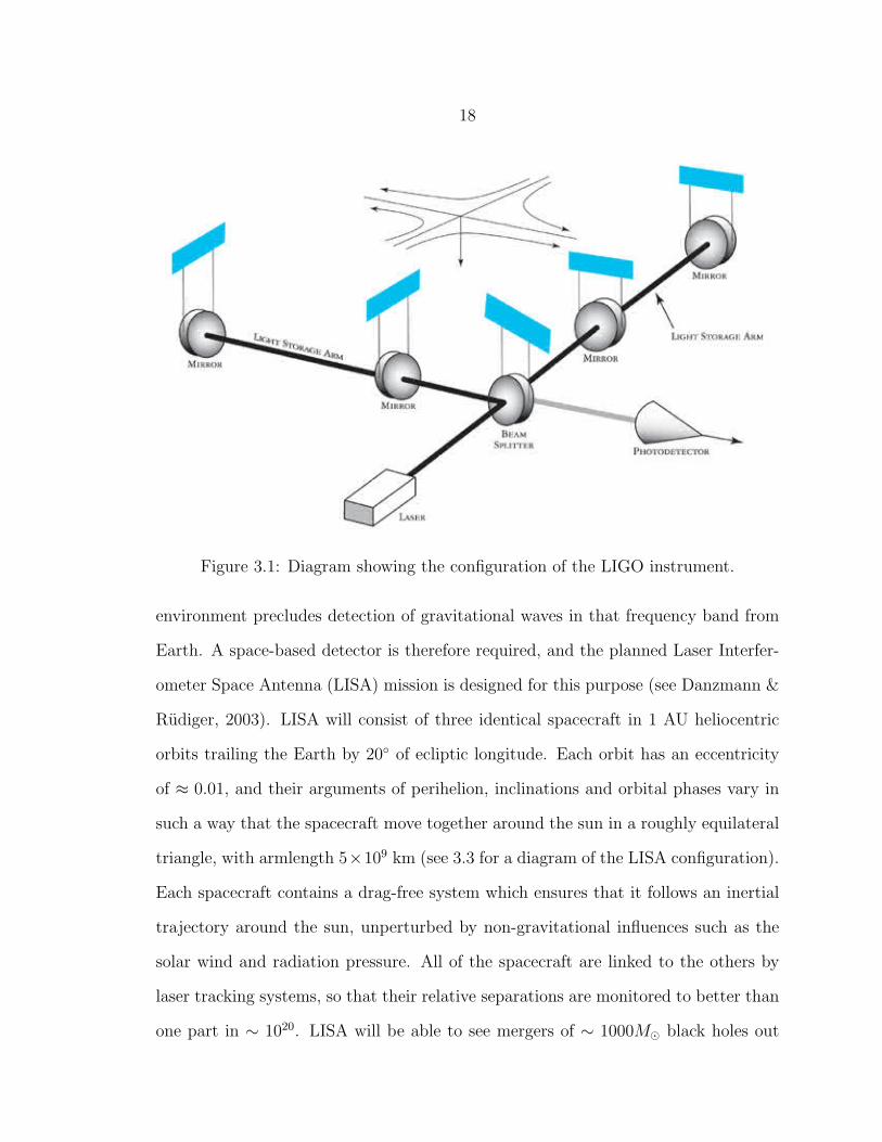
required, and these are only now beginning to come online. They are of the laser
interferometer type, where laser light is sent on a round trip along two distinct paths
which are at some angle to each other, and recombined on their return (see Figure
3.1). The resulting pattern of interference fringes is sensitive to differences in the
path lengths of the beams which are smaller than the wavelength of the laser light
(∼ 5 × 10⁻⁷ meters), and the location of the nulls in the interference fringes can be
measured with high accuracy. Thus, these detectors can reach the sensitivity needed
to measure the variation, caused by an astrophysical GW, of one part in ∼ 1020 in the
optical path length of the beams (Figure 3.2 shows the strain sensitivity attained by
initial LIGO’s 5th science run). The most sensitive current instruments, the LIGO
detectors, are not yet at the point where their expected event rates are ∼ 1yr−1
or better (Abbott et al., 2009). However, upgrades will soon begin(Smith & LIGO
Scientific Collaboration, 2009) which will bring LIGO to an ‘advanced’ configura-
tion, which has much higher sensitivity and is expected to see ∼ 10 events per year.
The frequency band covered by LIGO ranges from 10 . . . 10000 Hz, and so it will be
sensitive to coalescences of binaries containing white dwarfs, neutron stars or stellar
mass black holes, as well as to asymmetric supernovae and rapidly spinning pulsars
with ‘mountains’. Unfortunately, it is not sensitive to mergers of MBHs, as their
size places their maximum emitted frequencies below the LIGO sensitivity band (for
comparison, the fundamental ringdown frequency of a newly merged 1000M black
hole at z = 10 is ∼ 3 Hz).
Sensitivity to lower frequencies in the range of 10−4 . . . 10−1 Hz is required to ob-
serve the inspiral and coalescence of MBHs, but excessive noise due to the terrestrial
18
Figure 3.1: Diagram showing the configuration of the LIGO instrument.
environment precludes detection of gravitational waves in that frequency band from
Earth. A space-based detector is therefore required, and the planned Laser Interfer-
ometer Space Antenna (LISA) mission is designed for this purpose (see Danzmann &
Rudiger, 2003). LISA will consist of three identical spacecraft in 1 AU heliocentric
orbits trailing the Earth by 20 of ecliptic longitude. Each orbit has an eccentricity
of ≈ 0.01, and their arguments of perihelion, inclinations and orbital phases vary in
such a way that the spacecraft move together around the sun in a roughly equilateral
triangle, with armlength 5×10⁹ km (see 3.3 for a diagram of the LISA configuration).
Each spacecraft contains a drag-free system which ensures that it follows an inertial
trajectory around the sun, unperturbed by non-gravitational influences such as the
solar wind and radiation pressure. All of the spacecraft are linked to the others by
laser tracking systems, so that their relative separations are monitored to better than
one part in ∼ 1020. LISA will be able to see mergers of ∼ 1000M black holes out
19
10 100 1000 10000Frequency [Hz]
1e-24
1e-23
1e-22
1e-21
1e-20
1e-19
1e-18
1e-17
1e-16
h[f]
, 1/S
qrt[
Hz]
LHO 4km - (2007.03.18) S5: Binary Inspiral Range (1.4/1.4 Msun) = 15.6 Mpc
LLO 4km - (2007.08.30) S5: Binary Inspiral Range (1.4/1.4 Msun) = 16.2 Mpc
LHO 2km - (2007.05.14) S5: Binary Inspiral Range (1.4/1.4 Msun) = 7.5 Mpc
LIGO I SRD Goal, 4km
Strain Sensitivity of the LIGO InterferometersFinal S5 Performance LIGO-G0900957-v1
Figure 3.2: Strain sensitivity achieved by the 5th science run of the initial LIGOinstrument. This graph can be found in (Smith & LIGO Scientific Collaboration,2009), which also discusses anticipated sensitivity curves for advanced LIGO.
20
Figure 3.3: Diagram showing the orbits of the LISA constellation (not to scale).
to z ∼ 20 (Crowder & Cornish, 2006), so it is very well suited to observing MBH
populations. This dissertation therefore concentrates on LISA, although many of the
topics discussed are relevant to other detectors and/or source populations.
3.2 Production of Gravitational Waves
Calculating the detectability of binary systems emitting gravitational waves is a
standard problem in the gravitational wave community; see, for instance, Flanagan
& Hughes (1998a,b), and Cutler & Flanagan (1994). We review the problem here for
convenience and locality of reference.
First, an overview of Einstein’s General Theory of Relativity, which constitutes our
current understanding of gravity. This is reviewed in considerable detail in introduc-
tory textbooks on gravitation, such as (Schutz, 1985; Hartle, 2003); the derivation here
largely follows Hartle (2003). As is customary when working with General Relativity,
21
we use natural units where the speed of light and Newton’s gravitational constant are
unity, and the Einstein summation convention (index variables appearing twice in a
term are summed over) is in full effect unless otherwise stated.
The curvature of space-time, encapsulated in the Einstein tensor Gµν , is related
to the stress-energy-momentum tensor, Tµν , according to
Gµν = 8πTµν . (3.1)
The Einstein tensor is derived from the Ricci tensor Rµν and metric gµν according to
Gµν = Rµν −1
2gµνR, (3.2)
where the Ricci curvature scalar, R, is just the trace of the Ricci tensor. The Ricci
tensor is defined by a contraction of the Riemann curvature tensor, Rαβγδ:
Rµν ≡ Rαµαν . (3.3)
The Riemann curvature tensor describes how infinitesimally separated geodesics (the
paths travelled by unaccelerated test particles) diverge from each other due to the
curvature of space-time, and it is derived from the Christoffel symbols, Γαβγ:
Rαβγδ =∂Γα
βδ
∂xγ−∂Γα
βγ
∂xδ+ Γα
γεΓεβδ − Γα
δεΓεβγ (3.4)
The Christoffel symbols, in turn, describe how a vector changes when it is moved
around a space via parallel-transport, and are derived from the fundamental tensor
describing a spacetime, the metric gµν :
Γαβγ =
1
2gαδ
[∂gδβ
∂xγ+∂gδγ
∂xβ− ∂gβγ
∂xδ
](3.5)
The metric, finally, describes how the physical separation between two points in the
space-time is related to the coordinates of the points. Specifically, the line element
22
ds between a point x and a point infinitesimally separated from it by a coordinate
displacement dx is
ds2 = dxαdxβgαβ. (3.6)
The metric also provides the mapping from vectors to their dual vectors, represented
in the standard notation by whether the vector is indexed by a superscript or by a
subscript, and similarly for tensors. For instance, Rαβγδ is related to Rαβγδ (compare
equations 3.3 and 3.4) by
Rαβγδ = gαεRεβγδ. (3.7)
The Einstein equation then relates, via the complicated relationships defined
above, the components of the metric tensor of a space-time to the energy, momentum,
and stress contained in the space-time. It constitutes a system of 10 second-order cou-
pled, nonlinear, partial differential equations for gµν given Tµν . Needless to say, exact
analytical solutions of these equations are impossible for all but the simplest systems.
In fact, managing to produce a functioning numerical simulation of the general two-
body problem has required decades of heroic effort by modelers(For recent advances
in the two-body problem in GR, see Pretorius, 2005; Baker et al., 2006; Campanelli
et al., 2007). In contrast, the two-body problem in Newtonian gravity has been solved
analytically and is the subject of undergraduate mechanics texts, and production of
functioning numerical solutions for arbitrary numbers of bodies is trivial (although
their evaluation can be computationally expensive). The basics of gravitational-wave
production, propagation, and detection, however, are largely accessible with a far
simpler weak-field approximation, which we review next.
Let us suppose that the metric can be written as the sum of the flat space metric of
special relativity, ηµν = diag(−1, 1, 1, 1), plus a small perturbation hµν 1. Working
23
to first order in hµν , we have
gµν = ηµν + hµν . (3.8)
If we define a ‘trace-reversed’ amplitude as
hµν = hµν −1
2ηµνh
αα, (3.9)
then the Einstein equation reduces to
hµν = −16πTµν , (3.10)
where the D’alembertian or wave operator is equal to −∂2/∂t2+∇2. Thus, the com-
ponents of the metric obey standard wave equations with sources given by −16πTµν .
This equation is straightforward to solve using standard Green’s function techniques.
When this result is solved in the limit of long wavelengths for the fields far from the
source, it is found that the spatial (i.e., x, y, and z) components of the trace-reversed
metric amplitude are1
hij(t,x) =2
r
d2
dt2I ij(t− r), (3.11)
where the dependence on the stress-energy-momentum tensor, Tµν , has simplified to
(see Chapter 23 of Hartle, 2003) dependence on I ij, second mass moment of the source
(which has mass density ρ):
I ij =
∫d3xρ(t,x)xixj. (3.12)
In the case of a binary of reduced mass µ in a circular orbit in the x-y plane of
diameter d and orbital phase Φ, we have
I ij → µd2
2
1 + cos (2Φ) sin (2Φ) 0
sin (2Φ) 1− cos (2Φ) 0
0 0 0
. (3.13)
1We employ the convention that Latin indices refer only to spatial components, while Greek
indices refer to the full dimensions of the space-time.
24
To lowest non-vanishing order, the metric perturbation is then given by
hij → −4µd2Φ2
r
cos [2Φ(t− r)] sin [2Φ(t− r)] 0
sin [2Φ(t− r)] − cos [2Φ(t− r)] 0
0 0 0
. (3.14)
Thus, in a reference frame comoving with the source, the fundamental frequency of
the gravitational radiation, fs, is twice the orbital frequency, fs,orb ≡ Φs/(2π). At
this point, we use Kepler’s law to express the orbital separation, ds, in terms of fs,
and express the mass dependence in terms of the ‘chirp mass’:
Mc ≡ [m1 +m2]2/5 × µ3/5 (3.15)
The metric perturbation then becomes
hij → −8Mc
r
[πfsMc
]2/3
cos [2Φ(ts − r)] sin [2Φ(ts − r)] 0
sin [2Φ(ts − r)] − cos [2Φ(ts − r)] 0
0 0 0
. (3.16)
The orbit will gradually decay due to the power radiated in these gravitational waves
(see Peters & Mathews, 1963), with the result that the gravitational wave frequency
increases with time according to
dfs
dts=
96
5
fs
Mc
(πfsMc
)8/3. (3.17)
This describes the gravitational radiation of a circular, non-spinning binary to lowest
non-vanishing order in a frame that is comoving with the source. In practice, higher
order than linear terms are needed to characterize the waveform of a binary that
is nearing coalescence, but the above derivation illustrates how the process may be
carried out. First, the Einstein equations are evaluated, keeping terms up to some
order in the metric perturbation. Then, the gravitational radiation encapsulated in
25
the resulting metric is characterized, using expressions for the orbit evolution obtained
using post-Newtonian expansions. After that, the radiation reaction on the orbit due
to the emission of gravitational waves is determined. The new orbit can then be
used to add higher order corrections to the metric and the resulting radiation. This
process quickly becomes very mathematically cumbersome, and we do not attempt
to reproduce it here (see, for instance Blanchet, 2006). The waveforms used in this
work do employ higher order corrections, however. The spinning BHB code used
in Chapter 6 is valid to 2PN order (i.e, [v/c]4) in both amplitude and phase (Arun
et al., 2009), while the LISA calculator code used in Chapter 5 is valid to 2PN order
in phase and lowest order in amplitude, but assumes zero spin.
3.3 Detection of Gravitational Waves
We now consider a signal in the frame of a detector situated (at distance r) with
azimuthal angle ψ and polar angle ι with respect to the source. The cosmology is
such that the redshift between the source and detector is z, which alters the source’s
observed amplitude and frequency variation. In terms of the detector-frame variables,
we note that f = fs/(1 + z) and t = ts(1 + z), so that
f =96
5
f
Mc(1 + z)
(πfMc(1 + z)
)8/3. (3.18)
Writing the geometrical distance, r, in terms of the luminosity distance, DL, the
gravitational wave amplitude becomes
−8Mc(1 + z)
DL
[πfMc(1 + z)
]2/3. (3.19)
Thus, observing the chirp of a binary (the ramping up of its frequency with time) de-
termines its redshifted chirp mass, Mc(1+z), and observing the amplitude determines
26
its luminosity distance (although somewhat poorly since it is strongly correlated with
the binary’s inclination and sky location). Mc always appears in the GW signal
accompanied by a factor of (1 + z), so only the redshifted chirp mass can be inferred
from observation of the gravitational wave. In general, all dimensionful mass variables
appearing in the GW signal are redshifted, and the rest frame masses of the binaries
cannot be inferred directly from the signal. If a particular cosmology is assumed, the
redshift can be inferred from the luminosity distance, but this adds significant error
to the determination of the mass (it may be possible to constrain the redshift of a
binary by observing an optical counterpart, however). Unless otherwise specified, we
use redshifted mass variables from this point onwards.
Since we have restricted our attention to the case of circular orbits, we can take
advantage of this and, choosing the y axis to be orthogonal to the line of sight, rotate
the x and z axes about the y axis so that the z direction is along the line of sight
(i.e. the direction of propagation of the wave). Following the prescription given in
(Chapter 21 of Hartle, 2003), the spatial part (hij) of the metric perturbation in the
transverse-traceless gauge2 at the detector is
−4Mc
DL
[πfMc
]2/3
(1 + cos2 ι) cos [2Φ(f)] 2 cos ι sin [2Φ(f)] 0
2 cos ι sin [2Φ(f)] −(1 + cos2 ι) cos [2Φ(f)] 0
0 0 0
, (3.20)
2GR possesses a gauge freedom corresponding to a particular choice of coordinate system. In
particular, we can add to each of the coordinates, xα, an arbitrary small function ξα(x), without
resulting in any change in the physics of the system. It turns out that these ξα can be chosen so that
only the metric perturbation components transverse to the propagation direction are non-zero and
the metric perturbation has zero trace. The result is imaginatively named the transverse-traceless
gauge.
27
and the other components of the metric perturbation (i.e., hµ0 or h0ν) are zero. In
equation 3.20, we have suppressed an initial gravitational-wave phase offset Φ0 and
written Φ as a function of the fundamental gravitational wave frequency f , which is
a function of time (see equation 3.18):
Φ(f) ≡∫ t
f(t′)dt′ + Φ0. (3.21)
Note that in the coordinate system of equation 3.20, the y axis remains in the plane
of the binary’s orbit, and points along the long axis of the apparent ellipse formed by
the binary’s circular orbit as viewed from the detector. It is customary to break the
gravitational wave apart into two independent polarization states whose amplitudes
h+ and h× are given by
h+(f) =4Mc [πfMc]
2/3
DL
(1 + cos2 ι) cos [2Φ(f)]
h×(f) = −8Mc [πfMc]2/3
DL
cos ι sin [2Φ(f)] . (3.22)
We can now write the full gravitational wave metric as
gµν →
−1 0 0 0
0 1− h+ −h× 0
0 −h× 1 + h+ 0
0 0 0 1
. (3.23)
The separations between two coordinate locations in the space-time of the GW
are determined by the metric. For instance, the physical space-time interval, ∆s,
between two events at xa and xb measured along a locus of points with coordinates
specified by the set of functions xµ(λ) is determined by integrating the line elements
(specified by the metric tensor) over the path between the points (compare equation
3.6):
∆s =
∫ λb
λa
√gµν
dxµ
dλ
dxν
dλdλ (3.24)
28
For purposes of LISA’s measurement of the GW, we are interested in photon
times-of-flight along one arm of the interferometer. This can be found by determining
the null geodesic (i.e., ds2 = 0) trajectories connecting the transmitting spacecraft (at
time of transmission) to the receiving spacecraft (at time of reception), and integrating
the dt2 given by equation 3.6 along the trajectory. This takes a simple form in
the special case of flat background spacetimes in Minkowski coordinates, with the
spacecraft at rest with respect to the coordinate system (i.e., the coordinates of the
spacecraft are constant), and with the GW perturbation expressed in the Transverse-
Traceless gauge (see Finn, 2009; Cornish, 2009). In this case, the time delay due to
the gravitational wave can be written:
δt =∆xi∆xj
2L2(1−∆z/L)
∫ τb
τa
hij(τ)dτ, (3.25)
where ∆x ≡ xa − xb, L ≡ |∆x|, τ = t − z determines the gravitational wave phase,
and the wave propagates along the z axis as before. It has only recently been realized
that this simple form applies only to the rather restricted conditions described above
(see again, Finn, 2009; Cornish, 2009), and care must be taken when making similar
calculations. One must ensure that the above conditions are satisfied when using this
result. Fortunately, the conditions can be satisfied in the case of GW detection with
LISA.
If we consider a circular (in the unperturbed metric) ring of test masses, the
effect of the gravitational wave is to affect the distances between the test masses into
those for an ellipse, with the strength of the distortion and the orientation of the
ellipse varying in time in a way that depends on the relative strength of h+ and h×
(see Figure 3.4). It is important to note that, in the transverse-traceless gauge, the
29
Figure 3.4: The effects of the h+ (top) and h× (bottom) gravitational wave polariza-tions on the distances between a circular ring of test masses.
coordinates of the test masses themselves are not ‘moved’ (i.e., accelerated) in any
way by the GW; it is only the distances between the test masses that change.
For gravitational waves far from a general source, the polarization amplitudes h+
and h× can be expanded in terms of harmonics as
h+,×(τ) =∑
n
h(n)+,× exp[inΦ(τ)], (3.26)
where τ is now given by τ = t− k ·~x, which locates the surface of constant phase for a
gravitational wave propagating in a general direction k. When the binary is far from
coalescence, the dominant emission is the n = 2 quadrupole, and the polarization
amplitudes take the form of equation 3.22.
30
3.4 LISA Detection
In the case of LISA, the orientations of the arms will vary as the spacecraft orbits
the sun, and the measured distances between the 3 arms, as given by equation 3.25,
are thus a complicated function of time. In the low-frequency limit, however, the
phase of a signal in the interferometer is directly proportional to the amplitude of the
wave. The response of the LISA detector to the two polarizations of a gravitational
wave from a binary can then be written as
y(τ) = F+(θ, φ, ι, ψ, τ)h+(τ) + F×(θ, φ, ι, ψ, τ)h×(τ), (3.27)
where F+ and F× are the LISA form factors that depend on the position (θ,φ) and
orientation (ι,ψ) of the source relative to the time-dependent LISA configuration.
These are discussed in, for instance, Moore & Hellings (2002).
One measure of the ability of the LISA detector to observe a binary signal is the
signal-to-noise ratio, defined as
(SNR)2 = 4
∫ ∞
0
|h(f)|2
SLISA(f)df , (3.28)
where |h(f)|2 = |h+(f)|2 + |h×(f)|2, with h+(f) and h×(f) being the Fourier trans-
forms of the polarization amplitudes in equation 3.22, and where SLISA(f) is the
apparent noise level of LISA’s Standard Curve Generator (Larson (2000), hereafter
SCG), an estimate that averages the LISA response over the entire sky and over all
polarization states and divides the LISA instrument noise, Sn(f), by this averaged
response.
Previous treatment of LISA observations of binary black hole populations (Sesana
et al., 2007) have employed this measure of detectability, while other treatments
(Sesana et al., 2004) have used a characteristic strain hc, following the prescription
31
of Thorne (1987). In this measure, the raw strain h of a source is multiplied by the
average number of cycles of radiation emitted over a frequency interval ∆f = 1/Tobs
centred at frequency f . The amplitude of the characteristic strain is then compared
directly against the 1-year averaged strain sensitivity curve from the SCG to produce
an SNR. In either case, a source is considered detectable if the resulting SNR exceeds
some standard threshold value (typically between 5 and 10).
While interesting for planning LISA data analysis pipelines, these SNR estimates
fail to address the fact that a detection is of little use for comparison with astrophysical
theory if the parameters of the binary are poorly determined. In particular, unless
the masses and redshifts of the detected black holes are measured, the observations
cannot be compared with the black-hole evolution models. A more complete analysis
that incorporates the effects of uncertainty in the binary parameters is required.
Parameter error estimation for black hole binaries detected via gravitational wave
emission has been discussed by many researchers (Cutler & Flanagan, 1994; Vallisneri,
2008; Moore & Hellings, 2002; Crowder, 2006). The following is a review of the
covariance analysis for a linear least squares process, based on the Fisher information
matrix, the method which forms the core of the error analysis in this work.
Let us suppose that the LISA combined data stream consists of discrete samples
of a signal given by (Eq. 3.27), with added noise:
sα = yα(λi) + nα (3.29)
Here, λi are the parameters of the source and nα is the noise, assumed to be stationary
and Gaussian. The probability distribution of the αth data point is therefore
p(sα|λi) =1√2πσ2
α
× e−12[sα−yα(λi)]
2/σ2α , (3.30)
32
where σα (with Greek subscript) is the standard deviation of the noise in the αth
data point.
The likelihood function for a particular data set, with parameters λi, is the product
of the probabilities (Eq. 3.30) for each data point. It is
L(sα|λj) ∝ exp
[−
∑i
1
2
[sα − yα(λj)]2
σ2α
](3.31)
The set of parameters, λi, that maximizes the likelihood function is an unbiased
estimate of the the set of actual model parameters, λi. To calculate the λi, we assume
that the differences between the estimated values and the true values, ∆λi ≡ λi − λi
are small enough that yα(λi) can be approximated by its first-order Taylor series
expansion about λi:
yα(λk) ≈ yα(λk) +∇iyα∆λi. (3.32)
where ∇i represents the partial derivative with respect to λi. This first-order expan-
sion is valid when the SNR is high enough, and the degree of correlation between the
parameters is low enough that the resulting ∆λi are small. Using Eq. 3.31 we find3
that the likelihood is maximized by
∆λi = (F−1)ij
∑α
1
2
(sα − yα)∇jyα
σ2α
, (3.33)
where the matrix F is the Fisher information matrix, with components
Fij =∑
α
1
2σ2α
∇iyα∇jyα. (3.34)
The expected parameter covariance matrix is
〈∆λi∆λj〉 = F−1ij (3.35)
3It is also necessary to keep only terms that are first order in the inverse of the SNR; see Vallisneri
(2008)
33
The standard deviations in each detected parameter, σi (with Latin subscript), are
given by the diagonal elements of the covariance matrix:
σ2i = F−1
ii (no sum over i) (3.36)
It is important to remember that the Fisher error estimate is accurate only when the
parameter uncertainties are small compared to the characteristic scales of the system
being fit (Vallisneri & Mock LISA Data Challenge Taskforce, 2006), a condition that
is not well satisfied for all of the binaries being modelled here. In these cases, however,
the method tends to overestimate the degree of uncertainty in systems with a sharply-
defined minimum, and the resulting error estimates tend to be conservative.
Rather than write our own Fisher error estimation codes, we have made use of two
codes. One is the LISA Calculator (Crowder & Cornish, 2006; Crowder, 2006). The
LISA Calculator uses the same instrument noise model Sn(f) that is used as input
to the SCG, and an analytic signal model similar to that discussed here (although
the frequency evolution incorporates some higher order terms). The LISA calculator
(Crowder & Cornish, 2006) executes quickly, but its signal model is relatively simple
(it lacks higher harmonics of the waveform) and it assumes circular, nonspinning
binaries. It is accurate to second Post-Newtonian order (i.e., v4/c4) in the binary
phase evolution, and lowest order otherwise. This is the code used to construct the
error kernels in Chapter 5. In Chapter 6, we use the recent Montana/MIT group
code, discussed in Arun et al. (2009), which was provided to us by Neil Cornish and
Scott Hughes. This waveforms used by this code (based on Apostolatos et al., 1994)
incorporate the effects of higher harmonics in the wave form, spins and spin precession,
but it executes much more slowly than the LISA calculator, so it is computationally
impractical to use it to calculate error kernels (defined in Chapter 5). It is accurate
to second Post-Newtonian order.
34
In either case, the codes take as input a set of source parameter values, λj, and
output a set of standard deviations (equation 3.36), σi, for the detected parameter
values, λi. Each detected parameter, λi, is assumed to have a Gaussian probability
density with mean λi and standard deviation σi,
pD(λi|λi) =1√2πσ2
i
exp
[−
[λi − λi
]2
2σ2i
]. (3.37)
A primary focus of this dissertation is using such error distributions to assess the
distinguishability of MBH population models as they would be seen by LISA. In the
next section, we consider and categorize the various source parameters which effect
the signal of a Black Hole Binary (BBH) detected by LISA.
Note that equation 3.37 neglects the (sometimes large) correlations between the
parameter estimation errors, effectively assuming that the axes of the error ellipse are
parallel to the parameter directions. In cases where the parameter estimation errors
are strongly correlated, this exaggerates the effects of the errors. In Chapter 6, how-
ever, we find that only one parameter (namely, χ2) has errors which significantly effect
the estimated parameter distributions predicted by the models, so this simplification
should not affect the results presented here. Also note that we are only considering
parameter estimation errors due to noise in the LISA instrument; other sources of
noise, such as variations in the amplitudes due to weak gravitational lensing effects,
are not included.
3.5 BBH Parameters & their Errors
Each black hole binary may be characterized by a number of parameters, which are
sometimes divided into two categories. The first category is the intrinsic parameters
which have to do with the local properties of the binary in its rest frame. They arem1,
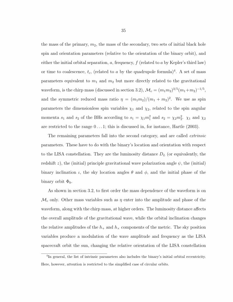
35
the mass of the primary, m2, the mass of the secondary, two sets of initial black hole
spin and orientation parameters (relative to the orientation of the binary orbit), and
either the initial orbital separation, a, frequency, f (related to a by Kepler’s third law)
or time to coalescence, tc, (related to a by the quadrupole formula)4. A set of mass
parameters equivalent to m1 and m2 but more directly related to the gravitational
waveform, is the chirp mass (discussed in section 3.2), Mc = (m1m2)3/5(m1+m2)
−1/5,
and the symmetric reduced mass ratio η = (m1m2)/(m1 + m2)2. We use as spin
parameters the dimensionless spin variables χ1 and χ2, related to the spin angular
momenta s1 and s2 of the BHs according to s1 = χ1m21 and s2 = χ2m
22. χ1 and χ2
are restricted to the range 0 . . . 1; this is discussed in, for instance, Hartle (2003).
The remaining parameters fall into the second category, and are called extrinsic
parameters. These have to do with the binary’s location and orientation with respect
to the LISA constellation. They are the luminosity distance DL (or equivalently, the
redshift z), the (initial) principle gravitational wave polarization angle ψ, the (initial)
binary inclination ι, the sky location angles θ and φ, and the initial phase of the
binary orbit Φ0.
As shown in section 3.2, to first order the mass dependence of the waveform is on
Mc only. Other mass variables such as η enter into the amplitude and phase of the
waveform, along with the chirp mass, at higher orders. The luminosity distance affects
the overall amplitude of the gravitational wave, while the orbital inclination changes
the relative amplitudes of the h+ and h× components of the metric. The sky position
variables produce a modulation of the wave amplitude and frequency as the LISA
spacecraft orbit the sun, changing the relative orientation of the LISA constellation
4In general, the list of intrinsic parameters also includes the binary’s initial orbital eccentricity.
Here, however, attention is restricted to the simplified case of circular orbits.
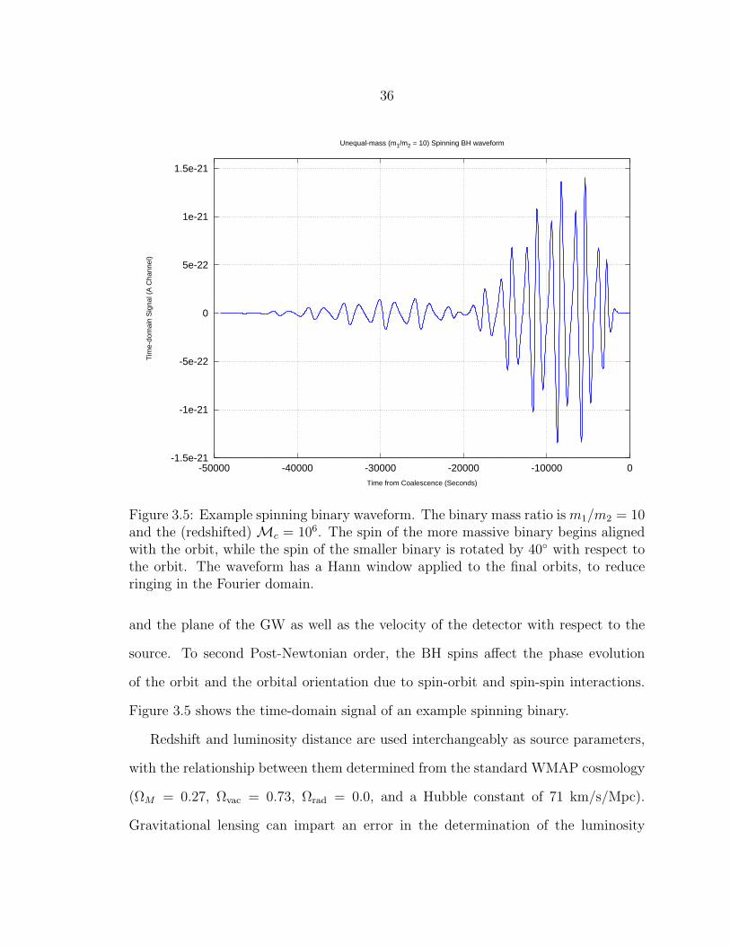
36
-1.5e-21
-1e-21
-5e-22
0
5e-22
1e-21
1.5e-21
-50000 -40000 -30000 -20000 -10000 0
Tim
e-do
mai
n S
igna
l (A
Cha
nnel
)
Time from Coalescence (Seconds)
Unequal-mass (m1/m2 = 10) Spinning BH waveform
Figure 3.5: Example spinning binary waveform. The binary mass ratio is m1/m2 = 10and the (redshifted) Mc = 106. The spin of the more massive binary begins alignedwith the orbit, while the spin of the smaller binary is rotated by 40 with respect tothe orbit. The waveform has a Hann window applied to the final orbits, to reduceringing in the Fourier domain.
and the plane of the GW as well as the velocity of the detector with respect to the
source. To second Post-Newtonian order, the BH spins affect the phase evolution
of the orbit and the orbital orientation due to spin-orbit and spin-spin interactions.
Figure 3.5 shows the time-domain signal of an example spinning binary.
Redshift and luminosity distance are used interchangeably as source parameters,
with the relationship between them determined from the standard WMAP cosmology
(ΩM = 0.27, Ωvac = 0.73, Ωrad = 0.0, and a Hubble constant of 71 km/s/Mpc).
Gravitational lensing can impart an error in the determination of the luminosity
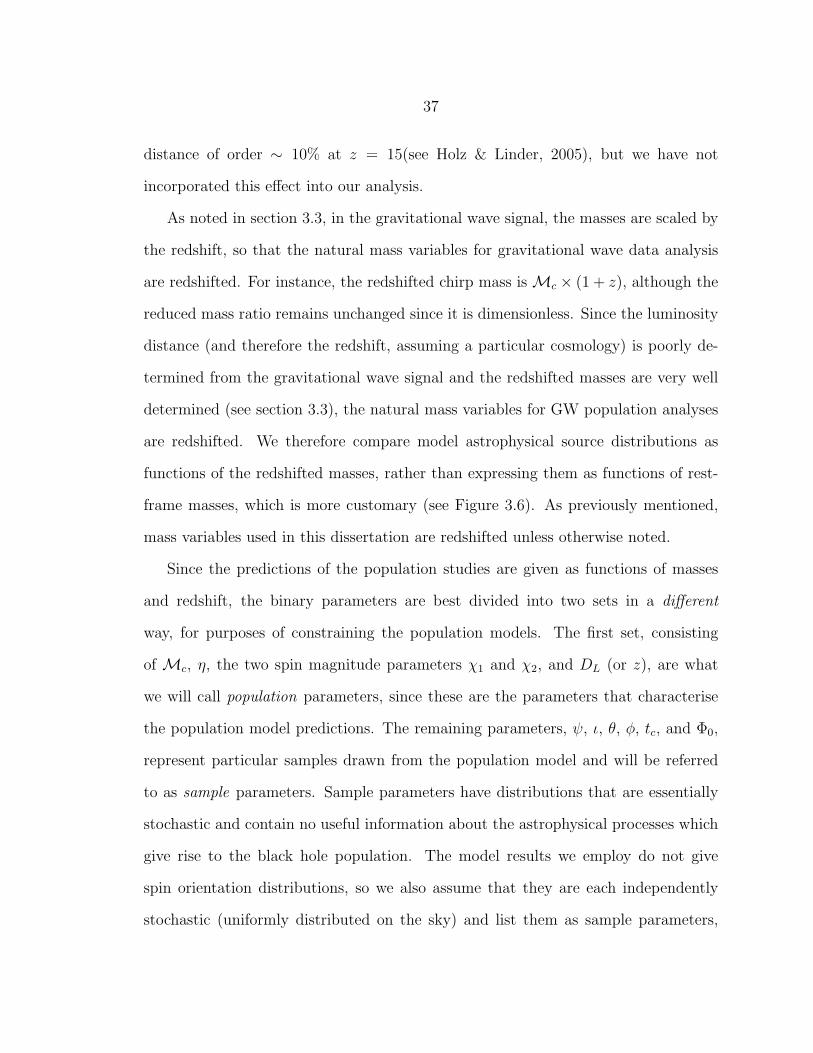
37
distance of order ∼ 10% at z = 15(see Holz & Linder, 2005), but we have not
incorporated this effect into our analysis.
As noted in section 3.3, in the gravitational wave signal, the masses are scaled by
the redshift, so that the natural mass variables for gravitational wave data analysis
are redshifted. For instance, the redshifted chirp mass is Mc × (1 + z), although the
reduced mass ratio remains unchanged since it is dimensionless. Since the luminosity
distance (and therefore the redshift, assuming a particular cosmology) is poorly de-
termined from the gravitational wave signal and the redshifted masses are very well
determined (see section 3.3), the natural mass variables for GW population analyses
are redshifted. We therefore compare model astrophysical source distributions as
functions of the redshifted masses, rather than expressing them as functions of rest-
frame masses, which is more customary (see Figure 3.6). As previously mentioned,
mass variables used in this dissertation are redshifted unless otherwise noted.
Since the predictions of the population studies are given as functions of masses
and redshift, the binary parameters are best divided into two sets in a different
way, for purposes of constraining the population models. The first set, consisting
of Mc, η, the two spin magnitude parameters χ1 and χ2, and DL (or z), are what
we will call population parameters, since these are the parameters that characterise
the population model predictions. The remaining parameters, ψ, ι, θ, φ, tc, and Φ0,
represent particular samples drawn from the population model and will be referred
to as sample parameters. Sample parameters have distributions that are essentially
stochastic and contain no useful information about the astrophysical processes which
give rise to the black hole population. The model results we employ do not give
spin orientation distributions, so we also assume that they are each independently
stochastic (uniformly distributed on the sky) and list them as sample parameters,
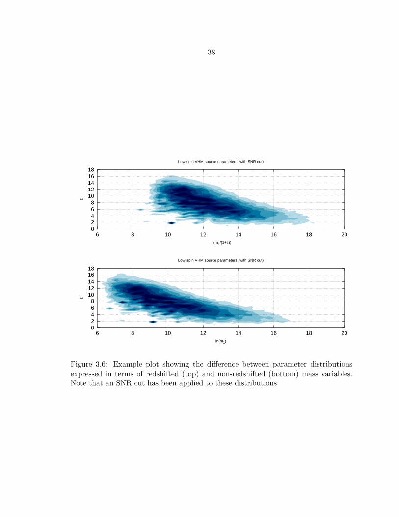
38
z
ln(m1/(1+z))
Low-spin VHM source parameters (with SNR cut)
02468
1012141618
6 8 10 12 14 16 18 20
z
ln(m1)
Low-spin VHM source parameters (with SNR cut)
02468
1012141618
6 8 10 12 14 16 18 20
Figure 3.6: Example plot showing the difference between parameter distributionsexpressed in terms of redshifted (top) and non-redshifted (bottom) mass variables.Note that an SNR cut has been applied to these distributions.
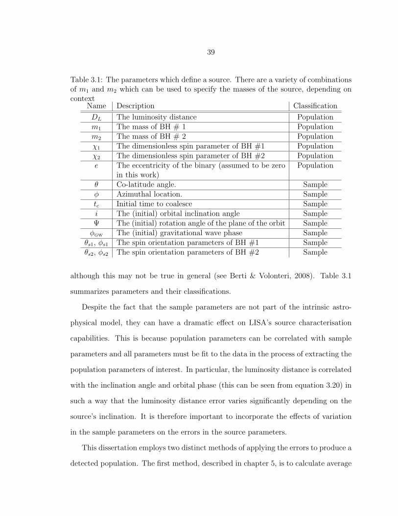
39
Table 3.1: The parameters which define a source. There are a variety of combinationsof m1 and m2 which can be used to specify the masses of the source, depending oncontext
Name Description Classification
DL The luminosity distance Populationm1 The mass of BH # 1 Populationm2 The mass of BH # 2 Populationχ1 The dimensionless spin parameter of BH #1 Populationχ2 The dimensionless spin parameter of BH #2 Populatione The eccentricity of the binary (assumed to be zero
in this work)Population
θ Co-latitude angle. Sampleφ Azimuthal location. Sampletc Initial time to coalesce Samplei The (initial) orbital inclination angle SampleΨ The (initial) rotation angle of the plane of the orbit SampleφGW The (initial) gravitational wave phase Sample
θs1, φs1 The spin orientation parameters of BH #1 Sampleθs2, φs2 The spin orientation parameters of BH #2 Sample
although this may not be true in general (see Berti & Volonteri, 2008). Table 3.1
summarizes parameters and their classifications.
Despite the fact that the sample parameters are not part of the intrinsic astro-
physical model, they can have a dramatic effect on LISA’s source characterisation
capabilities. This is because population parameters can be correlated with sample
parameters and all parameters must be fit to the data in the process of extracting the
population parameters of interest. In particular, the luminosity distance is correlated
with the inclination angle and orbital phase (this can be seen from equation 3.20) in
such a way that the luminosity distance error varies significantly depending on the
source’s inclination. It is therefore important to incorporate the effects of variation
in the sample parameters on the errors in the source parameters.
This dissertation employs two distinct methods of applying the errors to produce a
detected population. The first method, described in chapter 5, is to calculate average
40
LISA error distributions for the population parameters by averaging over a Monte
Carlo ensemble of many sources, each having randomly-chosen values for the sample
parameters. Such error distributions are referred to as ‘error kernels’. The second
method, described in the Chapter 6, generates a new set of random sample parameters
for every source in a realization of a population. It has the advantage, compared to
the error kernel, that it is easier to implement and the up-front computational cost is
quite low. It also scales easily to the case where there are more than a few population
parameters, while the error kernel does not. On the other hand, once error kernels are
computed, new realizations of a LISA detected parameter set can be produced very
quickly. The error kernel also provides a convenient way to visualize LISA’s average
parameter determination error (see Figure 5.1).
41
CHAPTER 4
MODEL COMPARISON
A data set is a collection of information that results from observations made with
some instrument. This information is represented as a series of data points, Ai, each
point describing a source or event found by the observations. In this work, each data
point is a set of best-fit parameters for a source found in a realization of the LISA data
stream. Our objective is to simulate such data sets for the various population models
and consider whether or not their differences are statistically significant. Comparing
a pair of data sets to see if they are drawn from the same population is a standard
problem in statistical analysis. For instance, section 14.3 of Press et al. (2002) states:
“Given two sets of data, we can generalize the questions asked in the
previous section and ask the single question, ‘Are the two sets drawn from
the same distribution function, or from different distribution functions?’
Equivalently, in proper statistical language, ‘Can we disprove, to a certain
required level of significance, the null hypothesis that the data sets are
drawn from the same population distribution functions?’”
In the traditional frequentist picture, which we use here, a ‘statistic’ is proposed
which quantifies the differences between the two data sets (call them A and B). In
the case of the familiar chi-squared test, the parameter space is divided into bins and
the statistic is found by taking the differences between the counts nA,i and nB,i in
each bin, normalizing them by the combined counts in the bins, and summing the
result:
χ2 =∑
i
(nA,i − nB,i)2
nA,i + nB,i
(4.1)
Then the question is asked,
42
Suppose that these two data sets were drawn from the same distribu-
tion, and the same experiment performed a large number of times. With
what frequency, p, would one obtain values of the statistic at least as
extreme as that which we actually observed?
If this p is low, we conclude that the data are unlikely to have been drawn from the
same population, and quantify our level of confidence in the result as (1− p)× 100%.
In other words, the confidence level is the cumulative distribution function (CDF) of
the test statistic in the case of the null hypothesis that both data sets were drawn
from the same population. For simple test statistics, this CDF is relatively easy to
calculate. In the case of the χ2 statistic, for instance, the CDF is an incomplete
gamma function (see Press et al., 2002, section 14.3), as plotted in Figure 4.1. For
more complicated test statistics, the CDF can be found by calculating the statistics for
Monte Carlo draws of two data sets which are both drawn from the same distribution
(consistent with the null nypothesis), a technique employed in this chapter.
4.1 The 1-D K-S Test and Variants
The tests used in this work are based on the Kolmogorov-Smirnov (K-S) test. Its
nonparametric and unbinned nature makes it well suited to the sparsely distributed
(∼ 100 sources spread over multiple decades and parameter dimensions) MBH popu-
lation, unlike the binned χ2 test. In practice, however, it is restricted to distributions
which are functions of at most two parameters. The analysis performed in Chapter
6 uses various choices for those two parameters, applying the tests to comparisons
of astrophysical model predictions for the distributions of best-fit parameters and
considering LISA’s model distinguishing power for each.
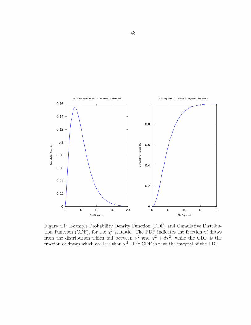
43
0
0.02
0.04
0.06
0.08
0.1
0.12
0.14
0.16
0 5 10 15 20
Pro
babi
lity
Den
sity
Chi Squared
Chi Squared PDF with 5 Degrees of Freedom
0
0.2
0.4
0.6
0.8
1
0 5 10 15 20
Cum
ulat
ive
Pro
babi
lity
Chi Squared
Chi Squared CDF with 5 Degrees of Freedom
Figure 4.1: Example Probability Density Function (PDF) and Cumulative Distribu-tion Function (CDF), for the χ2 statistic. The PDF indicates the fraction of drawsfrom the distribution which fall between χ2 and χ2 + dχ2, while the CDF is thefraction of draws which are less than χ2. The CDF is thus the integral of the PDF.
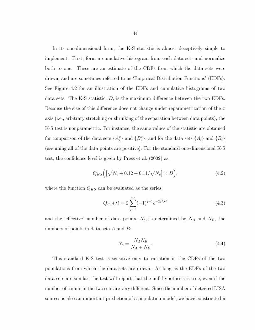
44
In its one-dimensional form, the K-S statistic is almost deceptively simple to
implement. First, form a cumulative histogram from each data set, and normalize
both to one. These are an estimate of the CDFs from which the data sets were
drawn, and are sometimes referred to as ‘Empirical Distribution Functions’ (EDFs).
See Figure 4.2 for an illustration of the EDFs and cumulative histograms of two
data sets. The K-S statistic, D, is the maximum difference between the two EDFs.
Because the size of this difference does not change under reparametrization of the x
axis (i.e., arbitrary stretching or shrinking of the separation between data points), the
K-S test is nonparametric. For instance, the same values of the statistic are obtained
for comparison of the data sets A2i and B2
i , and for the data sets Ai and Bi
(assuming all of the data points are positive). For the standard one-dimensional K-S
test, the confidence level is given by Press et al. (2002) as
QKS
([√Ne + 0.12 + 0.11/
√Ne
]×D
), (4.2)
where the function QKS can be evaluated as the series
QKS(λ) = 2∞∑
j=1
(−1)j−1e−2j2λ2
(4.3)
and the ‘effective’ number of data points, Ne, is determined by NA and NB, the
numbers of points in data sets A and B:
Ne =NANB
NA +NB
. (4.4)
This standard K-S test is sensitive only to variation in the CDFs of the two
populations from which the data sets are drawn. As long as the EDFs of the two
data sets are similar, the test will report that the null hypothesis is true, even if the
number of counts in the two sets are very different. Since the number of detected LISA
sources is also an important prediction of a population model, we have constructed a
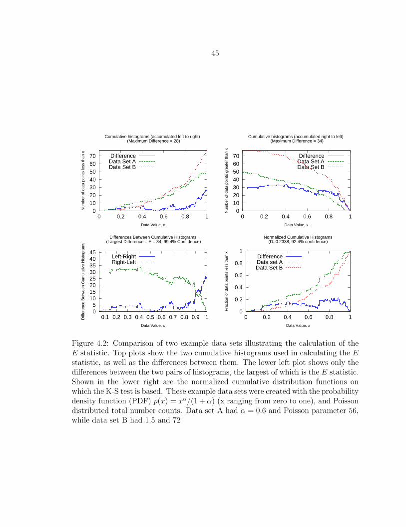
45
010203040506070
0 0.2 0.4 0.6 0.8 1
Num
ber
of d
ata
poin
ts g
reat
er th
an x
Data Value, x
Cumulative histograms (accumulated right to left) (Maximum Difference = 34)
DifferenceData Set AData Set B
05
1015202530354045
0.1 0.2 0.3 0.4 0.5 0.6 0.7 0.8 0.9 1Diff
eren
ce B
etw
een
Cum
ulat
ive
His
togr
ams
Data Value, x
Differences Between Cumulative Histograms (Largest Difference = E = 34, 99.4% Confidence)
Left-RightRight-Left
010203040506070
0 0.2 0.4 0.6 0.8 1
Num
ber
of d
ata
poin
ts le
ss th
an x
Data Value, x
Cumulative histograms (accumulated left to right) (Maximum Difference = 28)
DifferenceData Set AData Set B
0
0.2
0.4
0.6
0.8
1
0 0.2 0.4 0.6 0.8 1
Fra
ctio
n of
dat
a po
ints
less
than
x
Data Value, x
Normalized Cumulative Histograms(D=0.2338, 92.4% confidence)
DifferenceData set AData Set B
Figure 4.2: Comparison of two example data sets illustrating the calculation of theE statistic. Top plots show the two cumulative histograms used in calculating the Estatistic, as well as the differences between them. The lower left plot shows only thedifferences between the two pairs of histograms, the largest of which is the E statistic.Shown in the lower right are the normalized cumulative distribution functions onwhich the K-S test is based. These example data sets were created with the probabilitydensity function (PDF) p(x) = xα/(1 + α) (x ranging from zero to one), and Poissondistributed total number counts. Data set A had α = 0.6 and Poisson parameter 56,while data set B had 1.5 and 72
46
modified test that is also sensitive to differences in both the CDFs and the number
of sources. We begin by defining a new statistic, E, which differs from the K-S D
statistic most notably in that the cumulative histograms going into its calculation are
not normalized. Instead of ranging from 0 to 1, values of the statistic will range from
0 to NA and 0 to NB. Thus, significant differences in the total count rate can also lead
to significant differences in the statistic. We have found that using only the standard
cumulative histogram, which accumulates data counts going from left to right (low
to high data values), is sensitive primarily to distributions whose differences occur at
the upper end of the distribution, and insensitive to differences on the low end (the
upper two panels of Figure 4.2 illustrates this). In order to allow differences between
the model CDFs more opportunities to manifest themselves, we consider two sets of
differences between the data EDFs, one set with EDFs accumulated ranging from
small values of the data variable to large values, and the other set ranging from large
values to small values (see Figure 4.2). The statistic itself is taken to be the largest
difference found in the sets. Note that this statistic retains the useful nonparametric
nature of the standard K-S test. Then, we modify the null hypothesis:
Suppose that the two data sets are drawn from the same CDF, and
that the numbers of data points (i.e., the total number of sources) are
the result of a Poisson process with the same rate parameter. With what
frequency, p, would one obtain values of the E statistic at least as extreme
as that which we actually observed?
Rather than calculate the CDF of the test statistic analytically, we calculate it
numerically using Monte Carlo draws given this null hypothesis. Since the statistic
is nonparametric, our null hypothesis draws can use data points that are uniformly
distributed without loss of generality. Moreover, we have numerically determined
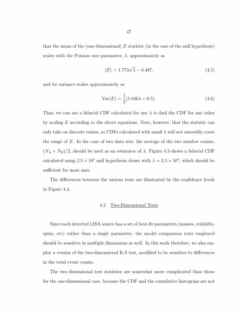
47
that the mean of the (one-dimensional) E statistic (in the case of the null hypothesis)
scales with the Poisson rate parameter, λ, approximately as
〈E〉 = 1.773√λ− 0.487, (4.5)
and its variance scales approximately as
Var(E) =1
2(1.046λ+ 0.5). (4.6)
Thus, we can use a fiducial CDF calculated for one λ to find the CDF for any other
by scaling E according to the above equations. Note, however, that the statistic can
only take on discrete values, so CDFs calculated with small λ will not smoothly cover
the range of E. In the case of two data sets, the average of the two number counts,
(NA +NB)/2, should be used as an estimator of λ. Figure 4.3 shows a fiducial CDF
calculated using 2.5× 10⁵ null hypothesis draws with λ = 2.5× 10⁴, which should be
sufficient for most uses.
The differences between the various tests are illustrated by the confidence levels
in Figure 4.4.
4.2 Two-Dimensional Tests
Since each detected LISA source has a set of best-fit parameters (masses, redshifts,
spins, etc) rather than a single parameter, the model comparison tests employed
should be sensitive in multiple dimensions as well. In this work therefore, we also em-
ploy a version of the two-dimensional K-S test, modified to be sensitive to differences
in the total event counts.
The two-dimensional test statistics are somewhat more complicated than those
for the one-dimensional case, because the CDF and the cumulative histogram are not
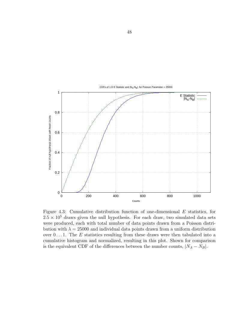
48
0
0.2
0.4
0.6
0.8
1
0 200 400 600 800 1000
Fra
ctio
n of
nul
l hyp
othe
sis
draw
s w
ith fe
wer
cou
nts
Counts
CDFs of 1-D E Statistic and |NA-NB|, for Poisson Parameter = 25000
E Statistic|NA-NB|
Figure 4.3: Cumulative distribution function of one-dimensional E statistics, for2.5 × 105 draws given the null hypothesis. For each draw, two simulated data setswere produced, each with total number of data points drawn from a Poisson distri-bution with λ = 25000 and individual data points drawn from a uniform distributionover 0 . . . 1. The E statistics resulting from these draws were then tabulated into acumulative histogram and normalized, resulting in this plot. Shown for comparisonis the equivalent CDF of the differences between the number counts, |NA −NB|.
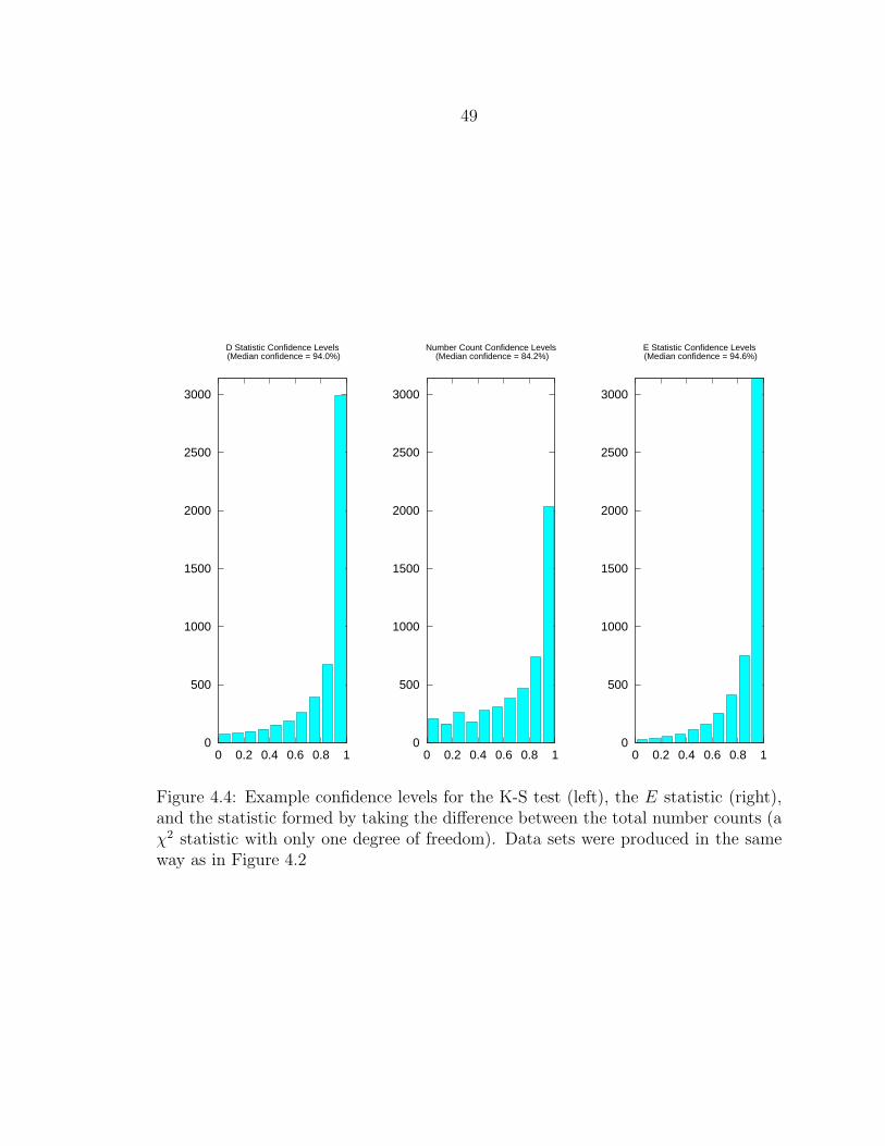
49
0
500
1000
1500
2000
2500
3000
0 0.2 0.4 0.6 0.8 1
D Statistic Confidence Levels (Median confidence = 94.0%)
0
500
1000
1500
2000
2500
3000
0 0.2 0.4 0.6 0.8 1
E Statistic Confidence Levels (Median confidence = 94.6%)
0
500
1000
1500
2000
2500
3000
0 0.2 0.4 0.6 0.8 1
Number Count Confidence Levels (Median confidence = 84.2%)
Figure 4.4: Example confidence levels for the K-S test (left), the E statistic (right),and the statistic formed by taking the difference between the total number counts (aχ2 statistic with only one degree of freedom). Data sets were produced in the sameway as in Figure 4.2
50
well defined in two or more dimensions (there’s a well defined rank ordering in one
dimension, but not in two or more). However, a working surrogate can be obtained
in two dimensions (Peacock, 1983). For each data point (xAi, yAi) in the set A, find
the fractions (one for data set B, one for data set A) of data points in the four
quadrants defined by (x < xAi, y < yAi), (x < xAi, y > yAi), (x > xAi, y < yAi), and
(x > xAi, y > yAi), for data set A and for data set B. Then, find the point x, y and
choice of quadrant for which the difference between these fractions is the greatest. Do
the same thing, but running over each data point in B, rather than each data point
in A, and average the two fractions1. This is the two-dimensional D statistic, first
implemented in this fashion by Fasano & Franceschini (1987). The two-dimensional
E statistic is the same except that, in place of the fraction of data points in each
quadrant, we use the number of data points in each quadrant.
In the case of the null hypothesis, the distribution of the D statistic is very nearly
independent of the shape of the two-dimensional distribution of the data points (Press
et al., 2002), and this appears to be the case for the E statistic as well (see section
4.3). The confidence levels (i.e., the CDFs for draws given the null hypothesis) for
both D and E can be calculated using draws given the null hypothesis, as before.
For the D statistic, Press et al. (2002) give an equation (14.7.1) that can be used
to calculate the CDF (specifically, it gives 1 − CDFD), although it is only roughly
correct for confidence levels & 90% (see section 4.3):
P(D > Observed) = QKS ×
D√N
1 +√
1− r2(0.25− 0.75/√N)
(4.7)
where N = NANB/(NA + NB), and r depends on the Pearson’s linear correlation
coefficients, rA and rB, of the samples according to r =√
1.0− (r2A + r2
B)/2. QKS
is given in equation 4.3. The E statistic CDFs were determined by Monte Carlo
1Press et al. (2002) give an algorithmic definition in the C language, which may be more clear
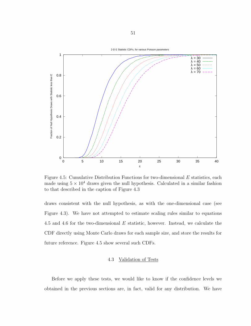
51
0
0.2
0.4
0.6
0.8
1
0 5 10 15 20 25 30 35 40
Fra
ctio
n of
Nul
l Hyp
othe
sis
Dra
ws
with
Sta
tistic
less
than
E
E
2-D E Statistic CDFs, for various Poisson parameters
λ = 30λ = 40λ = 50λ = 60λ = 70
Figure 4.5: Cumulative Distribution Functions for two-dimensional E statistics, eachmade using 5 × 10⁴ draws given the null hypothesis. Calculated in a similar fashionto that described in the caption of Figure 4.3
draws consistent with the null hypothesis, as with the one-dimensional case (see
Figure 4.3). We have not attempted to estimate scaling rules similar to equations
4.5 and 4.6 for the two-dimensional E statistic, however. Instead, we calculate the
CDF directly using Monte Carlo draws for each sample size, and store the results for
future reference. Figure 4.5 show several such CDFs.
4.3 Validation of Tests
Before we apply these tests, we would like to know if the confidence levels we
obtained in the previous sections are, in fact, valid for any distribution. We have
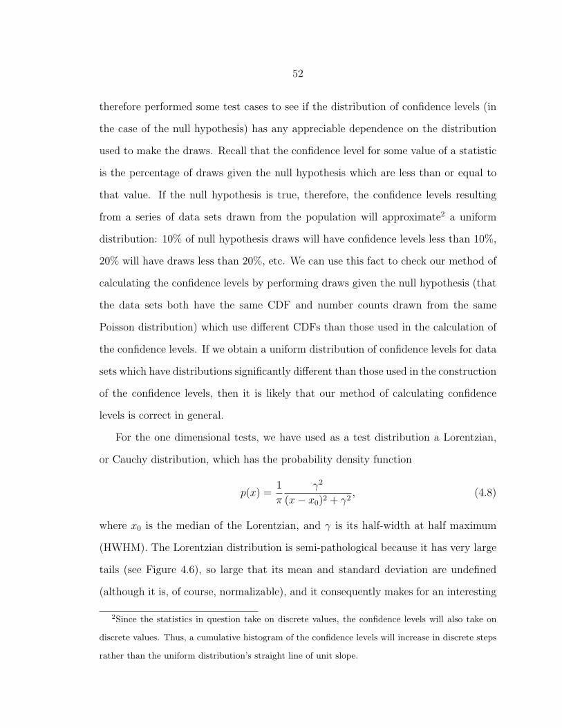
52
therefore performed some test cases to see if the distribution of confidence levels (in
the case of the null hypothesis) has any appreciable dependence on the distribution
used to make the draws. Recall that the confidence level for some value of a statistic
is the percentage of draws given the null hypothesis which are less than or equal to
that value. If the null hypothesis is true, therefore, the confidence levels resulting
from a series of data sets drawn from the population will approximate2 a uniform
distribution: 10% of null hypothesis draws will have confidence levels less than 10%,
20% will have draws less than 20%, etc. We can use this fact to check our method of
calculating the confidence levels by performing draws given the null hypothesis (that
the data sets both have the same CDF and number counts drawn from the same
Poisson distribution) which use different CDFs than those used in the calculation of
the confidence levels. If we obtain a uniform distribution of confidence levels for data
sets which have distributions significantly different than those used in the construction
of the confidence levels, then it is likely that our method of calculating confidence
levels is correct in general.
For the one dimensional tests, we have used as a test distribution a Lorentzian,
or Cauchy distribution, which has the probability density function
p(x) =1
π
γ2
(x− x0)2 + γ2, (4.8)
where x0 is the median of the Lorentzian, and γ is its half-width at half maximum
(HWHM). The Lorentzian distribution is semi-pathological because it has very large
tails (see Figure 4.6), so large that its mean and standard deviation are undefined
(although it is, of course, normalizable), and it consequently makes for an interesting
2Since the statistics in question take on discrete values, the confidence levels will also take on
discrete values. Thus, a cumulative histogram of the confidence levels will increase in discrete steps
rather than the uniform distribution’s straight line of unit slope.
53
test case. Rather than making all pairs of null hypothesis draws from identical distri-
butions, we have chosen a different set of random distribution parameters for each pair
of synthetic data sets drawn given the null hypothesis (naturally, each comparison
performed was between data sets with the same set of distribution parameters). The
Poisson rate parameters were chosen from a logarithmic distribution (rounded to the
nearest integer) ranging from 10 to 1000, and the Lorentzian median and HWHM
parameters were also chosen from logarithmic distributions ranging from 10 to 1000.
The results of 5000 such trial draws are shown in Figure 4.7, with the E statistic
confidence levels closely matching the expected uniform distribution. We have also
made draws with a reduced range of distribution parameters, to verify that variation
in the distribution parameters was not masking flaws in the confidence levels, but ob-
tained the same uniform distribution. This suggests that our E statistic confidence
levels are trustworthy, and that the nonparametric nature of the statistic does indeed
render it independent of the shape of the distribution. Curiously, the standard K-S
confidence levels exhibit a slight preference towards low confidence levels, for both the
Press et al. (2002) version (shown in Figure 4.7) and that used by the GNU Octave
software program.
For the two dimensional tests, one significant concern (see Peacock, 1983; Fasano
& Franceschini, 1987) is how the confidence levels are affected by the degree of corre-
lation in the data. We therefore use 3 test distributions. The first is a completely cor-
related Gaussian distribution along the line defined by θ = 45 (see Figure 4.8). The
second is partially correlated, and is composed of a pair of elongated two-dimensional
Gaussians, partially overlapping and rotated with respect to the x and y axes (see
Figure 4.9). The third is uncorrelated, and consists of a single circular two dimensional
Gaussian distribution (see Figure 4.10).
54
0
500
1000
1500
2000
2500
3000
-200 -100 0 100 200
Num
ber
Cou
nt
Data Value
Histogram of Lorentzian Distribution 50000 draws, HWHM = 48
Figure 4.6: Histogram of a Lorentzian Distribution. Draws falling outside of thedesignated histogram range have been placed into the outermost bins, illustrating thelarge tails of the distribution
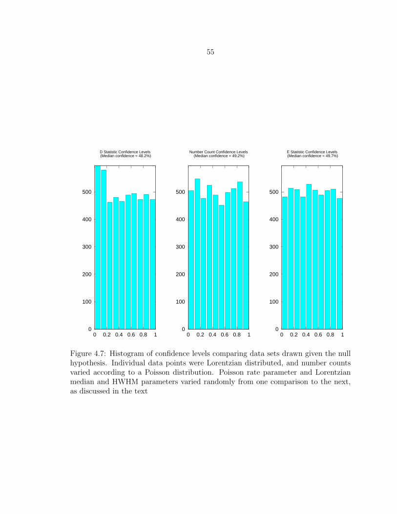
55
0
100
200
300
400
500
0 0.2 0.4 0.6 0.8 1
D Statistic Confidence Levels (Median confidence = 48.2%)
0
100
200
300
400
500
0 0.2 0.4 0.6 0.8 1
E Statistic Confidence Levels (Median confidence = 49.7%)
0
100
200
300
400
500
0 0.2 0.4 0.6 0.8 1
Number Count Confidence Levels (Median confidence = 49.2%)
Figure 4.7: Histogram of confidence levels comparing data sets drawn given the nullhypothesis. Individual data points were Lorentzian distributed, and number countsvaried according to a Poisson distribution. Poisson rate parameter and Lorentzianmedian and HWHM parameters varied randomly from one comparison to the next,as discussed in the text
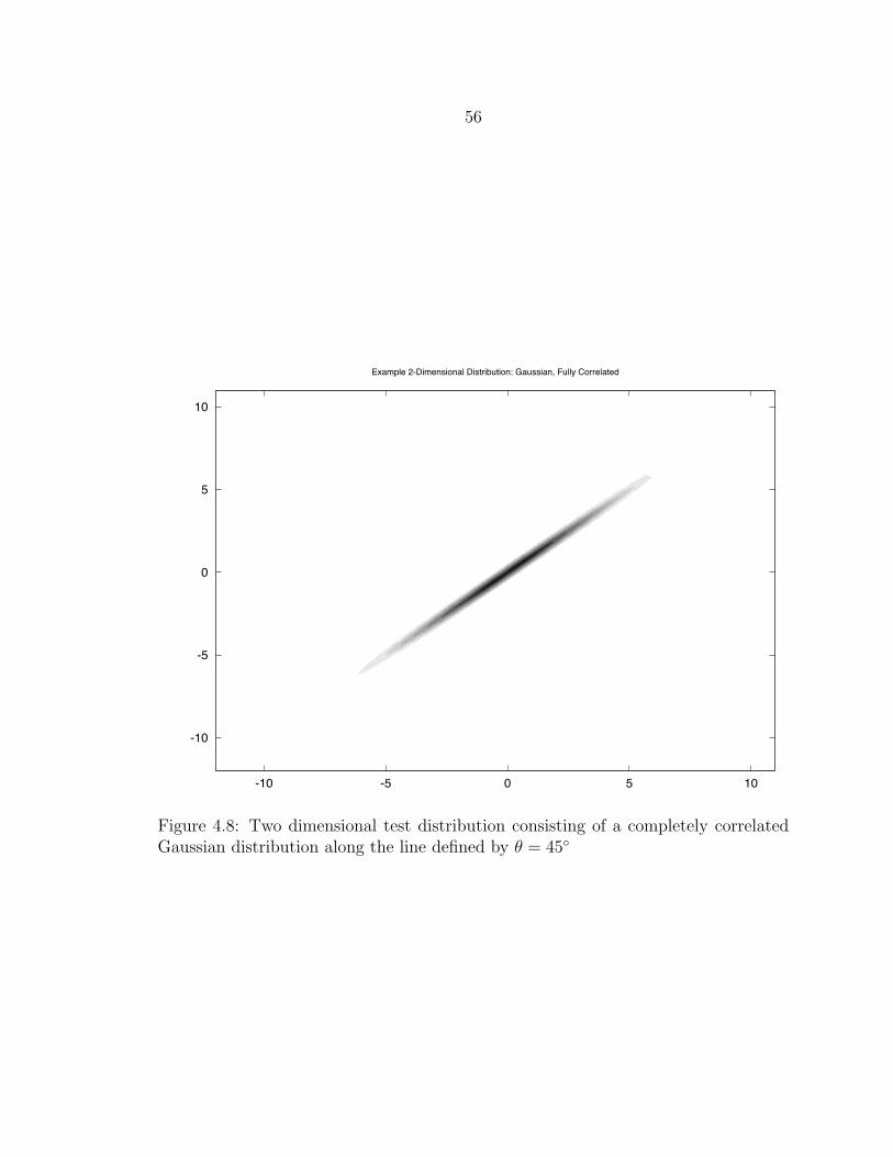
56
Example 2-Dimensional Distribution: Gaussian, Fully Correlated
-10
-5
0
5
10
-10 -5 0 5 10
Figure 4.8: Two dimensional test distribution consisting of a completely correlatedGaussian distribution along the line defined by θ = 45
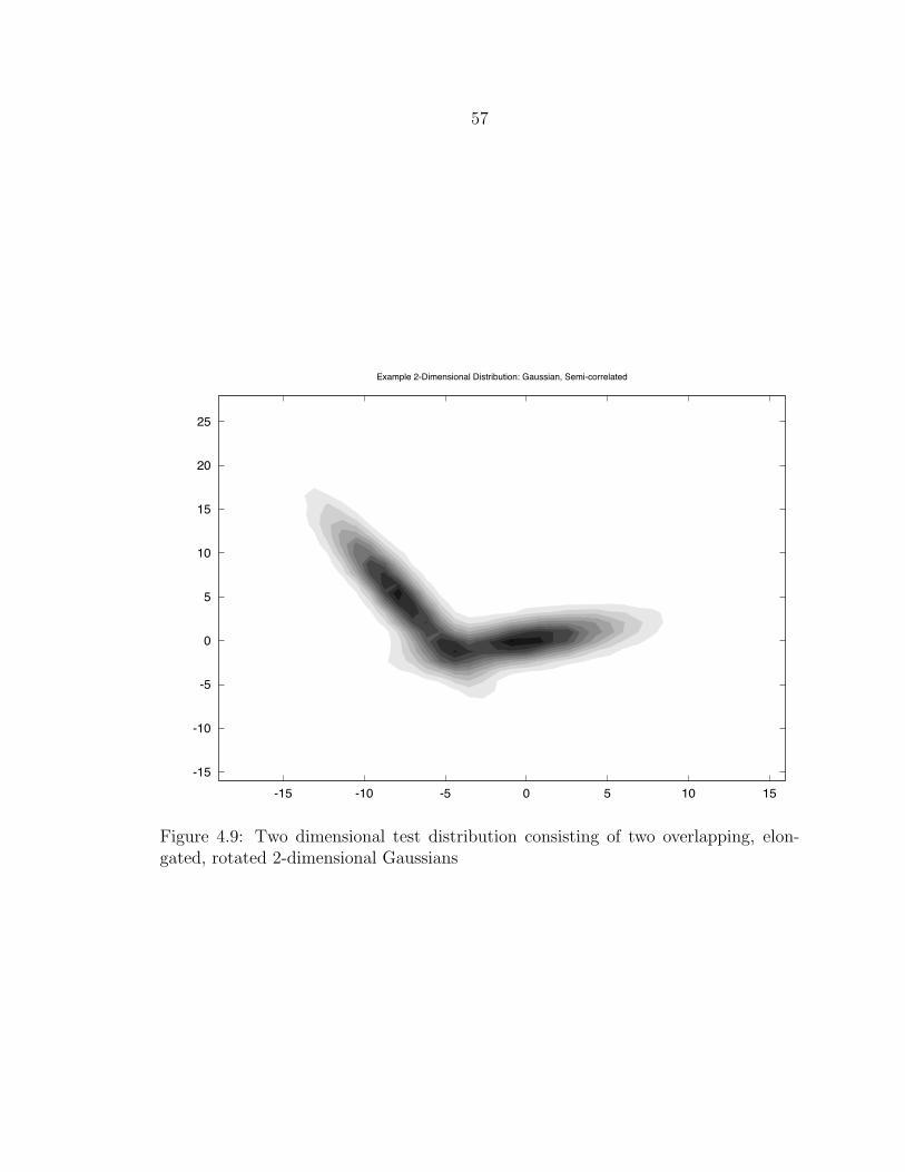
57
Example 2-Dimensional Distribution: Gaussian, Semi-correlated
-15
-10
-5
0
5
10
15
20
25
-15 -10 -5 0 5 10 15
Figure 4.9: Two dimensional test distribution consisting of two overlapping, elon-gated, rotated 2-dimensional Gaussians
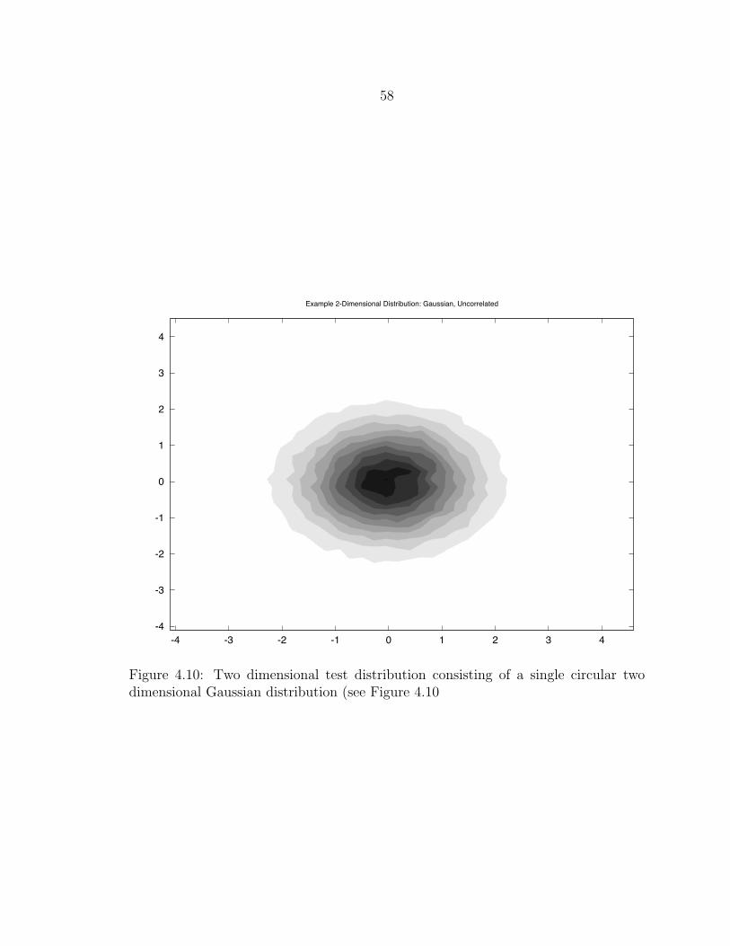
58
Example 2-Dimensional Distribution: Gaussian, Uncorrelated
-4
-3
-2
-1
0
1
2
3
4
-4 -3 -2 -1 0 1 2 3 4
Figure 4.10: Two dimensional test distribution consisting of a single circular twodimensional Gaussian distribution (see Figure 4.10
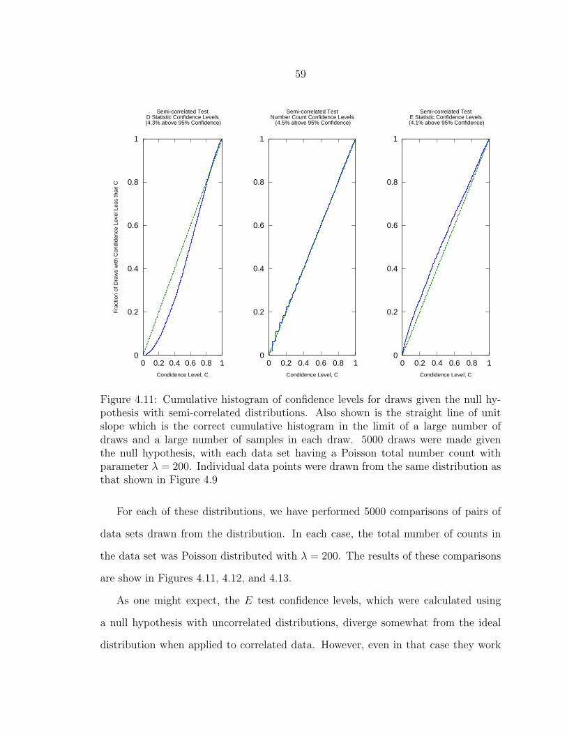
59
0
0.2
0.4
0.6
0.8
1
0 0.2 0.4 0.6 0.8 1
Fra
ctio
n of
Dra
ws
with
Con
dide
nce
Leve
l Les
s th
an C
Condidence Level, C
Semi-correlated TestD Statistic Confidence Levels
(4.3% above 95% Confidence)
0
0.2
0.4
0.6
0.8
1
0 0.2 0.4 0.6 0.8 1Condidence Level, C
Semi-correlated TestE Statistic Confidence Levels
(4.1% above 95% Confidence)
0
0.2
0.4
0.6
0.8
1
0 0.2 0.4 0.6 0.8 1Condidence Level, C
Semi-correlated TestNumber Count Confidence Levels
(4.5% above 95% Confidence)
Figure 4.11: Cumulative histogram of confidence levels for draws given the null hy-pothesis with semi-correlated distributions. Also shown is the straight line of unitslope which is the correct cumulative histogram in the limit of a large number ofdraws and a large number of samples in each draw. 5000 draws were made giventhe null hypothesis, with each data set having a Poisson total number count withparameter λ = 200. Individual data points were drawn from the same distribution asthat shown in Figure 4.9
For each of these distributions, we have performed 5000 comparisons of pairs of
data sets drawn from the distribution. In each case, the total number of counts in
the data set was Poisson distributed with λ = 200. The results of these comparisons
are show in Figures 4.11, 4.12, and 4.13.
As one might expect, the E test confidence levels, which were calculated using
a null hypothesis with uncorrelated distributions, diverge somewhat from the ideal
distribution when applied to correlated data. However, even in that case they work
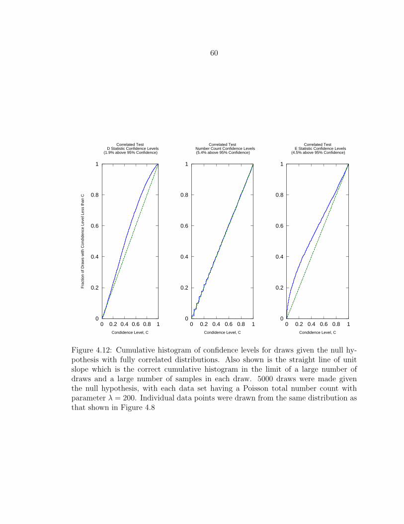
60
0
0.2
0.4
0.6
0.8
1
0 0.2 0.4 0.6 0.8 1
Fra
ctio
n of
Dra
ws
with
Con
dide
nce
Leve
l Les
s th
an C
Condidence Level, C
Correlated Test D Statistic Confidence Levels (1.9% above 95% Confidence)
0
0.2
0.4
0.6
0.8
1
0 0.2 0.4 0.6 0.8 1Condidence Level, C
Correlated Test E Statistic Confidence Levels (4.5% above 95% Confidence)
0
0.2
0.4
0.6
0.8
1
0 0.2 0.4 0.6 0.8 1Condidence Level, C
Correlated Test Number Count Confidence Levels
(5.4% above 95% Confidence)
Figure 4.12: Cumulative histogram of confidence levels for draws given the null hy-pothesis with fully correlated distributions. Also shown is the straight line of unitslope which is the correct cumulative histogram in the limit of a large number ofdraws and a large number of samples in each draw. 5000 draws were made giventhe null hypothesis, with each data set having a Poisson total number count withparameter λ = 200. Individual data points were drawn from the same distribution asthat shown in Figure 4.8
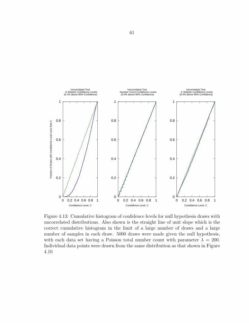
61
0
0.2
0.4
0.6
0.8
1
0 0.2 0.4 0.6 0.8 1
Fra
ctio
n of
Dra
ws
with
Con
dide
nce
Leve
l Les
s th
an C
Condidence Level, C
Uncorrelated Test D Statistic Confidence Levels (6.1% above 95% Confidence)
0
0.2
0.4
0.6
0.8
1
0 0.2 0.4 0.6 0.8 1Condidence Level, C
Uncorrelated Test E Statistic Confidence Levels (5.4% above 95% Confidence)
0
0.2
0.4
0.6
0.8
1
0 0.2 0.4 0.6 0.8 1Condidence Level, C
Uncorrelated Test Number Count Confidence Levels
(5.0% above 95% Confidence)
Figure 4.13: Cumulative histogram of confidence levels for null hypothesis draws withuncorrelated distributions. Also shown is the straight line of unit slope which is thecorrect cumulative histogram in the limit of a large number of draws and a largenumber of samples in each draw. 5000 draws were made given the null hypothesis,with each data set having a Poisson total number count with parameter λ = 200.Individual data points were drawn from the same distribution as that shown in Figure4.10

62
well in the range of 95 . . . 100% confidence. Since only confidence levels in that range
are considered statistically significant in any case, the E statistic confidence levels
are suitable for use in practice (compare Peacock, 1983). For the semi-correlated
case, the accuracy is much better, and it is nearly perfect for the uncorrelated case.
The number count confidence levels match the ideal distribution for all cases, but
this is trivially true, since it is completely insensitive to the distribution of data
points, and only considers the differences between the total number counts. The
2-Dimensional K-S test, as implemented from Press et al. (2002), does surprisingly
poorly, considering that it attempts to account for the degree of correlation between
the data sets. Although it never significantly over-estimates the confidence levels, it
appears to significantly underestimate the fraction of confidence levels over 95% in the
case of 100% correlated data. We have not investigated this further, however, because
the issue generally appears to make the standard K-S test more conservative, it is
widely accepted, and because our results are based on the E statistic comparisons.
We also perform the same check on each of the MBH population model results
discussed in Chapter 6 of this dissertation, in case the MBH parameter distributions
contain features which expose problems in the confidence level estimates which are
not revealed by the above tests. We find that, with 5000 comparisons made given
the null hypothesis for each model and combination of model parameters, the frac-
tion of confidence levels above 95% is very consistently within 0.04 and 0.06. This
indicates that our model comparison test performs correctly for the models used in
this dissertation.
63
CHAPTER 5
CONSTRAINING MBH POPULATIONS USING THE ERROR KERNEL
The output of the astrophysical models of interest can be described in terms of a
coalescence rate, Γ(M, η, z), per unit redshift and time. However, the coalescence rate
observed in the LISA detector, Γ′(M, η, z), will differ from Γ(M, η, z) because some
sources will be too weak to be detected and because errors in the LISA parameter
determination will assign incorrect parameters to the source, due to the effect of the
noise on the estimation process. The effect of these errors can be summed up in a
LISA ‘error kernel’, K:
Γ′(M, η, z) =
∫pop
Γ(M, η, z)× ε(M, η, z)
×K(M, η, z|M, η, z) dz dη dM, (5.1)
where ε(M, η, z) is the average detectability of a source with parameters M, η, z
in the LISA detector. This error kernel is the average conditional probability that a
source will be detected with population parameters λi in the LISA data, given the
existence of an astrophysical source with population parameters λi. The resulting
error kernels can be applied directly to model coalescence rates, producing a new set
of coalescence rates as functions of the best-fitting, ‘detected’, parameter values.
5.1 Calculating the Error Kernel
As discussed in section 3.5, coalescence rates given by the various models are
functions of the population parameters only. They do not depend on the sample
parameters, which arise from the random relationship between the observer and a
64
particular binary in the population. We therefore produce a Monte Carlo average
or ‘marginalisation’ over the sample parameters, compiling the Fisher matrix error
estimates into an ‘Error Kernel’ which is a function of sample parameters only.
Since we have no a priori reason to expect inhomogeneous or anisotropic distribu-
tion, the values of the extrinsic sample parameters of a black hole binary are assumed
to be uniformly distributed – angular location and orientation variables are uniformly
distributed on the sky, and Φ0 is uniformly distributed over the interval [0, 2π] (see
Table 5.1).
The appropriate distribution to use for tc is somewhat more complicated, owing to
two primary considerations. First, astrophysical models of the MBH population are
usually expressed in terms of the number of coalescences per unit time and redshift.
Second, the LISA detectability of a binary (generally related to SNR) is a monoton-
ically decreasing function of the binary’s tc (all else being equal) for tc longer than
the LISA observation time Tobs. Because of their relatively stronger signals, binaries
coalescing inside or soon after the LISA observation lifetime window are far more
likely to be detected than those with long times to coalescence, so those with long
times to coalescence represent a negligible fraction of the set of detected binaries. In
calculating the error kernel, we found that the number of additional detected sources
coalescing in the year following the end of LISA observation was a negligible fraction
of the total, and decided to simply use a 1 year observation time and range of tc for
most of our results, multiplying by 3 to get results for a 3 year observation. We found
that the results were not significantly different from, for instance, using a full 3 year
observation time and 4 year range of tc.
While the binary masses are also population parameters, the models we have
found in the literature generally divide their mass spectra into very wide logarithmic
bins or give no mass spectra at all. Since the mass also has a significant effect on
65
the detectability and parameter estimation error of a source, however, we cannot
simply generate masses completely at random or treat them in some other trivial
fashion. We therefore partially marginalize over the mass and attempt to make a
reasonable choice for the mass distribution within the mass bins published in the
literature. This choice of mass distribution is somewhat problematic, since additional
information on the mass distribution is available for some of the models studied
(Volonteri et al. (2003), for instance), but not for others. Even if useful information
on the mass distribution were available for all of the models studied, we prefer not
to tailor intra-bin mass distributions to each particular model, because we want the
error kernels to be model-independent. We have decided, for purposes of this work,
to use a simple uniform logarithmic distribution within each mass bin. While this
distribution can produce significant differences in detection rates for the coarsely-
binned models studied here, our opinion is that it remains a reasonable choice for a
model independent intra-bin mass distribution, and such problems are best solved by
increasing the mass resolution of the reported model results. For similar reasons, we
also completely marginalise over mass ratio. We use the three mass ranges found in
Sesana et al. (2007) for our mass bins. The redshift is not marginalised, and separate
Monte Carlo runs are made at uniformly spaced values of z ranging from 0 . . . 20 (see
Table 5.1) and the statistics are collected as a function of redshift. The ‘population’
parameter space is thus considered as a collection of two-dimensional volume elements
chosen from the three mass bins and up to 80 bins in redshift.
Within each volume element, values for the marginalised parameters are chosen
randomly and a covariance error analysis is performed, with the probability distri-
bution function (PDF) for each sample being calculated using Eq. 3.37. A typical
single PDF for one sample is shown in Figure 5.1a. PDFs from the random sampling
of the source parameters are stored and averaged, producing a PDF for the popu-
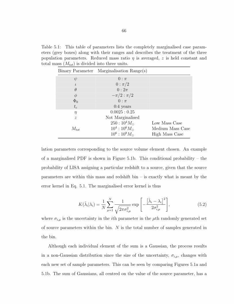
66
Table 5.1: This table of parameters lists the completely marginalised case param-eters (grey boxes) along with their ranges and describes the treatment of the threepopulation parameters. Reduced mass ratio η is averaged, z is held constant andtotal mass (Mtot) is divided into three units.
Binary Parameter Marginalisation Range(s)
ψ 0 : πι 0 : π/2θ 0 : 2πφ −π/2 : π/2Φ0 0 : πtc 0:4 yearsη 0.0025 : 0.25z Not Marginalised
Mtot
250 : 104M Low Mass Case104 : 106M Medium Mass Case106 : 108M High Mass Case
lation parameters corresponding to the source volume element chosen. An example
of a marginalised PDF is shown in Figure 5.1b. This conditional probability – the
probability of LISA assigning a particular redshift to a source, given that the source
parameters are within this mass and redshift bin – is exactly what is meant by the
error kernel in Eq. 5.1. The marginalised error kernel is thus
K(λi|λi) =1
N
N∑µ=1
1√2πσ2
i,µ
exp
[−
[λi − λi
]2
2σ2i,µ
], (5.2)
where σi,µ is the uncertainty in the ith parameter in the µth randomly generated set
of source parameters within the bin. N is the total number of samples generated in
the bin.
Although each individual element of the sum is a Gaussian, the process results
in a non-Gaussian distribution since the size of the uncertainty, σi,µ, changes with
each new set of sample parameters. This can be seen by comparing Figures 5.1a and
5.1b. The sum of Gaussians, all centred on the value of the source parameter, has a
67
taller peak and fatter tails than a single Gaussian with average standard deviation[∑Nµ=1 σ
2i,µ
]0.5/N .
There are two limitations in the way we have generated the error kernel that stem
from our use of the linear least-squares LISA Calculator. First, sources at moderate
redshift and large sigma will have tails that extend to low z, even though a true nearby
source would not be confused with a stronger source at moderate redshift. Production
of the true PDF for such a case would involve a more complete algorithm, avoiding
the limitations of linear least-squares analysis and resulting in a shorter low-z tail.
Second, the LISA Calculator, like many least-squares tools, drops an ill-determined
parameter when the information matrix is singular, and gives an inappropriately low
sigma for the remaining parameters. This did occur in a number of the cases we ran
and contributed some anomalously strong peaks to the Monte Carlo averaging.
Our covariance studies found that the fractional uncertainties in the redshifted
mass variables were always much less than the fractional uncertainties in redshift (see
Figure 5.2), and are insignificant compared to our coarse mass binning1. For the
purposes of this initial study, we have ignored the mass errors and considered only
the distribution of the detected redshifts. The error kernel is thus
Ki(z, z) =1
Ni
∑µi
1√2πσ2
z,µi
exp
[−(z − z)2
2σ2z,µi
], (5.3)
where i corresponds to one of the mass ranges defined in Table 5.1 and where the
sigmas are understood to be the uncertainties determined for each mass bin. Thus,
our Monte Carlo study returns three error kernels at a given redshift, one for each
mass range. Each error kernel consists of a set of PDFs, one PDF for each redshift bin
z. These source redshifts are uniformly spaced between 0 and 20 (see Figure 5.1c).
1Rest-frame variables with dimensions of mass will have an error that is 100% correlated with
the error in the redshift, a detail we will investigate in future work.
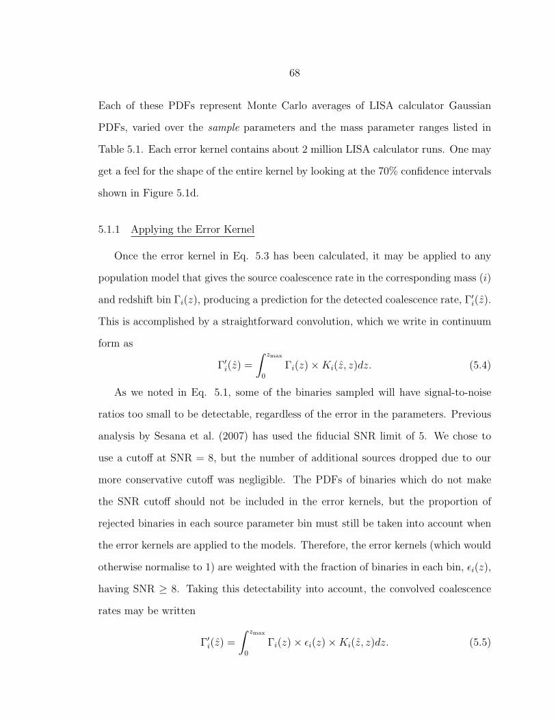
68
Each of these PDFs represent Monte Carlo averages of LISA calculator Gaussian
PDFs, varied over the sample parameters and the mass parameter ranges listed in
Table 5.1. Each error kernel contains about 2 million LISA calculator runs. One may
get a feel for the shape of the entire kernel by looking at the 70% confidence intervals
shown in Figure 5.1d.
5.1.1 Applying the Error Kernel
Once the error kernel in Eq. 5.3 has been calculated, it may be applied to any
population model that gives the source coalescence rate in the corresponding mass (i)
and redshift bin Γi(z), producing a prediction for the detected coalescence rate, Γ′i(z).
This is accomplished by a straightforward convolution, which we write in continuum
form as
Γ′i(z) =
∫ zmax
0
Γi(z)×Ki(z, z)dz. (5.4)
As we noted in Eq. 5.1, some of the binaries sampled will have signal-to-noise
ratios too small to be detectable, regardless of the error in the parameters. Previous
analysis by Sesana et al. (2007) has used the fiducial SNR limit of 5. We chose to
use a cutoff at SNR = 8, but the number of additional sources dropped due to our
more conservative cutoff was negligible. The PDFs of binaries which do not make
the SNR cutoff should not be included in the error kernels, but the proportion of
rejected binaries in each source parameter bin must still be taken into account when
the error kernels are applied to the models. Therefore, the error kernels (which would
otherwise normalise to 1) are weighted with the fraction of binaries in each bin, εi(z),
having SNR ≥ 8. Taking this detectability into account, the convolved coalescence
rates may be written
Γ′i(z) =
∫ zmax
0
Γi(z)× εi(z)×Ki(z, z)dz. (5.5)
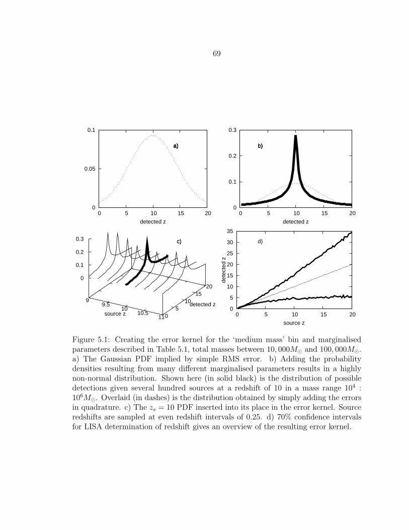
69
0
0.05
0.1
0 5 10 15 20
detected z
a)
0
0.1
0.2
0.3
0 5 10 15 20
detected z
a) b)
9 9.5
10 10.5
11 0 5
10 15
20
0
0.1
0.2
0.3
a) b)
c)
source z
detected z 0
5
10
15
20
25
30
35
0 5 10 15 20
dete
cted
z
source z
a) b)
c) d)
Figure 5.1: Creating the error kernel for the ‘medium mass’ bin and marginalisedparameters described in Table 5.1, total masses between 10, 000M and 100, 000M.a) The Gaussian PDF implied by simple RMS error. b) Adding the probabilitydensities resulting from many different marginalised parameters results in a highlynon-normal distribution. Shown here (in solid black) is the distribution of possibledetections given several hundred sources at a redshift of 10 in a mass range 104 :106M. Overlaid (in dashes) is the distribution obtained by simply adding the errorsin quadrature. c) The zs = 10 PDF inserted into its place in the error kernel. Sourceredshifts are sampled at even redshift intervals of 0.25. d) 70% confidence intervalsfor LISA determination of redshift gives an overview of the resulting error kernel.
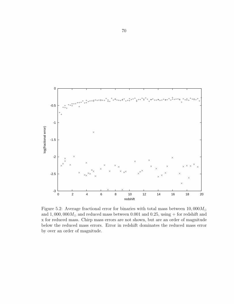
70
-3
-2.5
-2
-1.5
-1
-0.5
0
0 2 4 6 8 10 12 14 16 18 20
log(
frac
tiona
l err
or)
redshift
Figure 5.2: Average fractional error for binaries with total mass between 10, 000Mand 1, 000, 000M and reduced mass between 0.001 and 0.25, using + for redshift andx for reduced mass. Chirp mass errors are not shown, but are an order of magnitudebelow the reduced mass errors. Error in redshift dominates the reduced mass errorby over an order of magnitude.
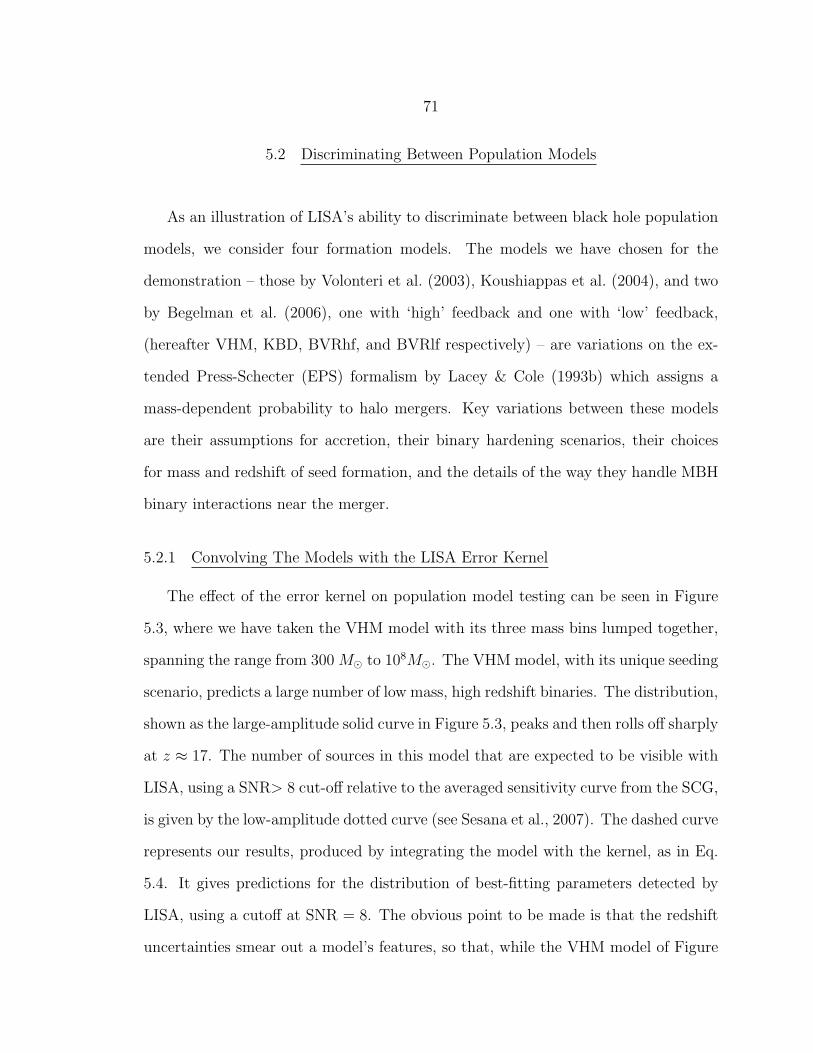
71
5.2 Discriminating Between Population Models
As an illustration of LISA’s ability to discriminate between black hole population
models, we consider four formation models. The models we have chosen for the
demonstration – those by Volonteri et al. (2003), Koushiappas et al. (2004), and two
by Begelman et al. (2006), one with ‘high’ feedback and one with ‘low’ feedback,
(hereafter VHM, KBD, BVRhf, and BVRlf respectively) – are variations on the ex-
tended Press-Schecter (EPS) formalism by Lacey & Cole (1993b) which assigns a
mass-dependent probability to halo mergers. Key variations between these models
are their assumptions for accretion, their binary hardening scenarios, their choices
for mass and redshift of seed formation, and the details of the way they handle MBH
binary interactions near the merger.
5.2.1 Convolving The Models with the LISA Error Kernel
The effect of the error kernel on population model testing can be seen in Figure
5.3, where we have taken the VHM model with its three mass bins lumped together,
spanning the range from 300 M to 108M. The VHM model, with its unique seeding
scenario, predicts a large number of low mass, high redshift binaries. The distribution,
shown as the large-amplitude solid curve in Figure 5.3, peaks and then rolls off sharply
at z ≈ 17. The number of sources in this model that are expected to be visible with
LISA, using a SNR> 8 cut-off relative to the averaged sensitivity curve from the SCG,
is given by the low-amplitude dotted curve (see Sesana et al., 2007). The dashed curve
represents our results, produced by integrating the model with the kernel, as in Eq.
5.4. It gives predictions for the distribution of best-fitting parameters detected by
LISA, using a cutoff at SNR = 8. The obvious point to be made is that the redshift
uncertainties smear out a model’s features, so that, while the VHM model of Figure

72
5.3 has a very distinctive shape in its theoretical incarnation, the distribution that
would be observed by LISA will be far less so.
The presence of detected sources at very low (z < 2) redshifts, where the VHM
population model says that there should be very few, is a result of the excessively
large low-z tails of the error kernel discussed in section 5.1. The less sharply peaked
shape of the error kernel results as compared with the Sesana results, however, is a
consquence of applying detection errors to the redshifts, and will persist even when
more robust error-estimation techniques are employed.
Even with our SNR cutoff, we predict more visible sources (179 vs. 96) than
did Sesana et al. (2007). This is due in part to our error kernel, with its use of
the logarithmic mass distributions within the large mass bins found in the literature,
having more massive binaries at high redshift than is actually the case for the VHM
models. We also found a discrepancy in Sesana et al. (2007) between their stated
event counts (∼ 250 for the VHM model with a 3 year range of coalescence times)
and the event counts found by integrating the curves in their figure 1 (over 400 for
the same case). We have consulted with Alberto Sesana on this subject and he has
confirmed that the discrepancy in the event counts is due to a mistaken factor in
the production of the plot. The correct figure is the 250 events listed in the text of
Sesana et al. (2007). Since our model event rates were obtained by extracting the
curves from that figure, this discrepancy could also contribute to the differing number
of visible sources.
5.2.2 Discriminating Between Models
For the four models we have chosen to consider as illustrative examples, the results
of the error kernel convolutions are shown in Figure 5.4. The graph in the upper left
is for all masses and the other three graphs represent the three mass bins we used.
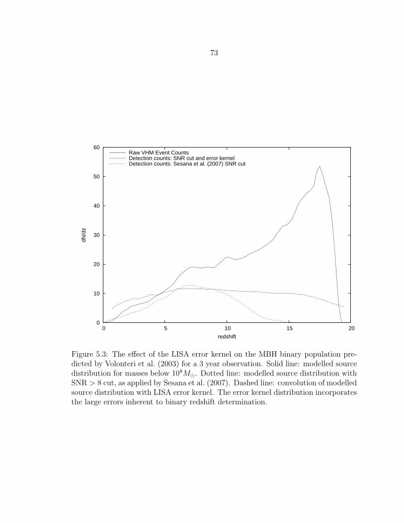
73
0
10
20
30
40
50
60
0 5 10 15 20
dN/d
z
redshift
Raw VHM Event CountsDetection counts: SNR cut and error kernelDetection counts: Sesana et al. (2007) SNR cut
Figure 5.3: The effect of the LISA error kernel on the MBH binary population pre-dicted by Volonteri et al. (2003) for a 3 year observation. Solid line: modelled sourcedistribution for masses below 108M. Dotted line: modelled source distribution withSNR > 8 cut, as applied by Sesana et al. (2007). Dashed line: convolution of modelledsource distribution with LISA error kernel. The error kernel distribution incorporatesthe large errors inherent to binary redshift determination.
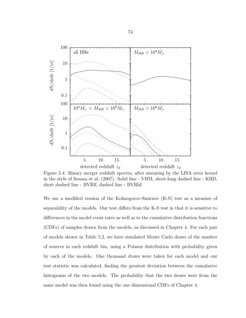
74
0.1
1
10
100
5 10 15
dN
/dzd
t[1
/yr]
detected redshift zd
104M < MBH < 106M
5 10 15
detected redshift zd
MBH > 106M
MBH < 104M
0.1
1
10
100dN
/dzd
t[1
/yr]
all BHs
Figure 5.4: Binary merger redshift spectra, after smearing by the LISA error kernelin the style of Sesana et al. (2007). Solid line - VHM, short-long dashed line - KBD,short dashed line - BVRlf, dashed line - BVRhf.
We use a modified version of the Kolmogorov-Smirnov (K-S) test as a measure of
separability of the models. Our test differs from the K-S test in that it is sensitive to
differences in the model event rates as well as to the cumulative distribution functions
(CDFs) of samples drawn from the models, as discussed in Chapter 4. For each pair
of models shown in Table 5.2, we have simulated Monte Carlo draws of the number
of sources in each redshift bin, using a Poisson distribution with probability given
by each of the models. One thousand draws were taken for each model and our
test statistic was calculated, finding the greatest deviation between the cumulative
histograms of the two models. The probability that the two draws were from the
same model was then found using the one dimensional CDFs of Chapter 4.
75
Several comparisons were done between the four models chosen from Sesana et al.
(2007). For each comparison, we assumed one year of LISA observations and randomly
drew coalescence parameters using the probability distributions for the two models
being compared. In each set of draws, our modified K-S statistic, E, was determined
andQ, the probability that two such draws would be produced by the same model, was
calculated. The results for each random draw were then averaged over one thousand
such realisations, giving the values displayed in Table 5.2. In the two data columns,
we show the results from the raw models themselves, with no parameter uncertainties
taken into account, and the results from the models after they have been convolved
with the LISA error kernel. As can be seen in the table, the probability that any
of the simulated data sets for one model might have been produced by one of the
other models is small. The models examined here appear to be easily distinguishable
from each other, with the exception of the comparison of the BVRhf model with
the BVRlf model with its average Q value of 0.055 (corresponding to a rather shaky
94.5% confidence). Even in that case, when we look at the median of Q rather than
its mean, we find it to be 0.012 (98.8% confidence), implying that a BVRlf realization
can usually be distinguished from a BVRhf realization.
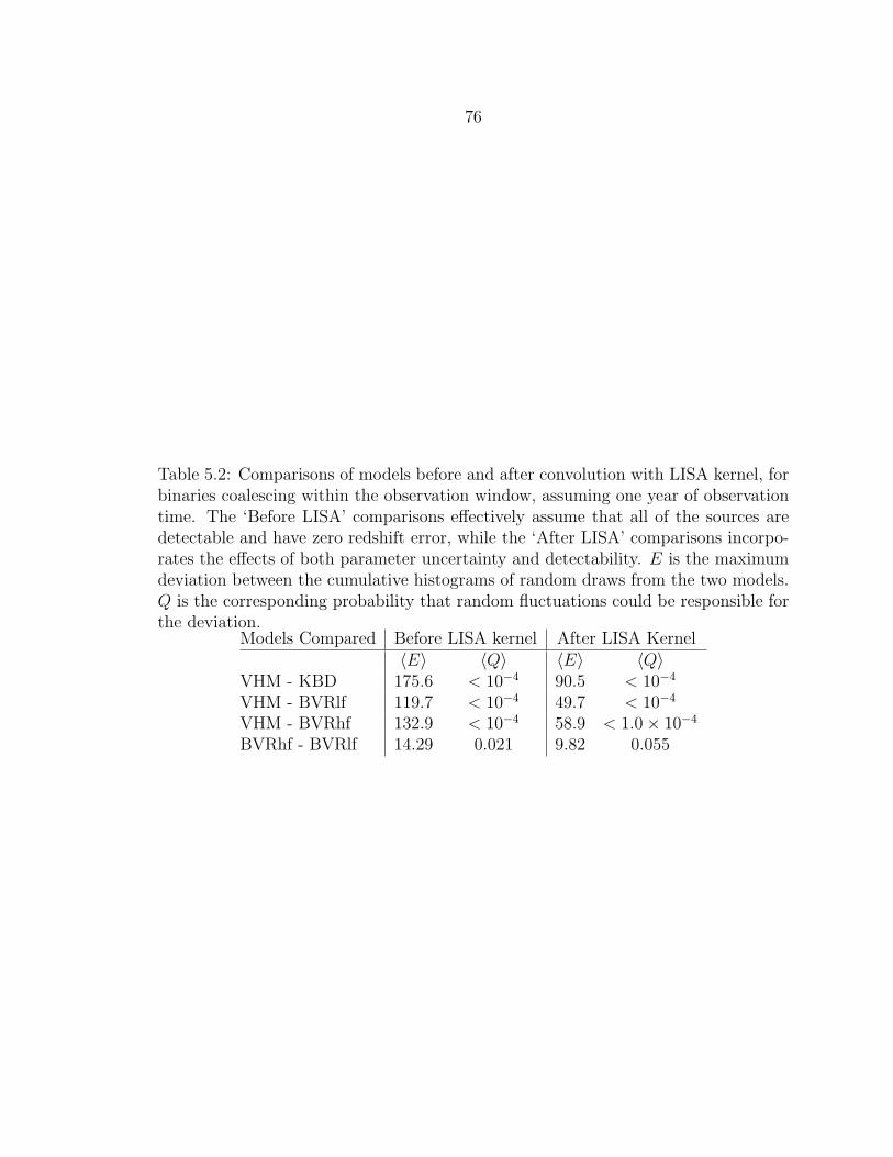
76
Table 5.2: Comparisons of models before and after convolution with LISA kernel, forbinaries coalescing within the observation window, assuming one year of observationtime. The ‘Before LISA’ comparisons effectively assume that all of the sources aredetectable and have zero redshift error, while the ‘After LISA’ comparisons incorpo-rates the effects of both parameter uncertainty and detectability. E is the maximumdeviation between the cumulative histograms of random draws from the two models.Q is the corresponding probability that random fluctuations could be responsible forthe deviation.
Models Compared Before LISA kernel After LISA Kernel〈E〉 〈Q〉 〈E〉 〈Q〉
VHM - KBD 175.6 < 10−4 90.5 < 10−4
VHM - BVRlf 119.7 < 10−4 49.7 < 10−4
VHM - BVRhf 132.9 < 10−4 58.9 < 1.0× 10⁻⁴
BVRhf - BVRlf 14.29 0.021 9.82 0.055
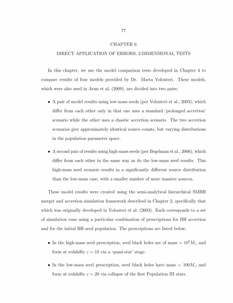
77
CHAPTER 6
DIRECT APPLICATION OF ERRORS; 2-DIMENSIONAL TESTS
In this chapter, we use the model comparison tests developed in Chapter 4 to
compare results of four models provided by Dr. Marta Volonteri. These models,
which were also used in Arun et al. (2009), are divided into two pairs:
• A pair of model results using low-mass seeds (per Volonteri et al., 2003), which
differ from each other only in that one uses a standard ‘prolonged accretion’
scenario while the other uses a chaotic accretion scenario. The two accretion
scenarios give approximately identical source counts, but varying distributions
in the population parameter space.
• A second pair of results using high-mass seeds (per Begelman et al., 2006), which
differ from each other in the same way as do the low-mass seed results. This
high-mass seed scenario results in a significantly different source distribution
than the low-mass case, with a smaller number of more massive sources.
These model results were created using the semi-analytical hierarchical SMBH
merger and accretion simulation framework described in Chapter 2, specifically that
which was originally developed in Volonteri et al. (2003). Each corresponds to a set
of simulation runs using a particular combination of prescriptions for BH accretion
and for the initial BH seed population. The prescriptions are listed below:
• In the high-mass seed prescription, seed black holes are of mass ∼ 105M and
form at redshifts z ∼ 10 via a ‘quasi-star’ stage.
• In the low-mass seed prescription, seed black holes have mass ∼ 100M and
form at redshifts z ∼ 20 via collapse of the first Population III stars.
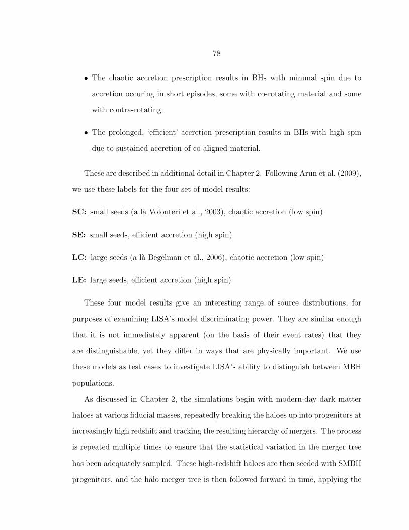
78
• The chaotic accretion prescription results in BHs with minimal spin due to
accretion occuring in short episodes, some with co-rotating material and some
with contra-rotating.
• The prolonged, ‘efficient’ accretion prescription results in BHs with high spin
due to sustained accretion of co-aligned material.
These are described in additional detail in Chapter 2. Following Arun et al. (2009),
we use these labels for the four set of model results:
SC: small seeds (a la Volonteri et al., 2003), chaotic accretion (low spin)
SE: small seeds, efficient accretion (high spin)
LC: large seeds (a la Begelman et al., 2006), chaotic accretion (low spin)
LE: large seeds, efficient accretion (high spin)
These four model results give an interesting range of source distributions, for
purposes of examining LISA’s model discriminating power. They are similar enough
that it is not immediately apparent (on the basis of their event rates) that they
are distinguishable, yet they differ in ways that are physically important. We use
these models as test cases to investigate LISA’s ability to distinguish between MBH
populations.
As discussed in Chapter 2, the simulations begin with modern-day dark matter
haloes at various fiducial masses, repeatedly breaking the haloes up into progenitors at
increasingly high redshift and tracking the resulting hierarchy of mergers. The process
is repeated multiple times to ensure that the statistical variation in the merger tree
has been adequately sampled. These high-redshift haloes are then seeded with SMBH
progenitors, and the halo merger tree is then followed forward in time, applying the
79
Table 6.1: The Press-Schechter weights, fiducial masses, and numbers of trees for themodel results compared in this chapter.
WPS nt M
0.006044 20 1.43× 10¹¹
0.003393 20 2.66× 10¹¹
0.001944 20 4.96× 10¹¹
0.001117 20 9.24× 10¹¹
0.000639 20 1.72× 10¹²
0.000363 20 3.20× 10¹²
0.000205 20 5.96× 10¹²
0.000116 20 1.11× 10¹³
6.570× 10−05 20 2.07× 10¹³
3.718× 10−05 20 3.85× 10¹³
4.330× 10−05 10 1× 10¹⁴
2.701× 10−06 5 1× 10¹⁵
prescriptions for MBH merging and accretion as the simulation proceeds. Each set
of model results consists of 12 files, one for each fiducial halo mass, Mi, which list
all of the mergers that occurred during the simulation runs for that halo mass. The
probability that, during some time interval ∆t, a source corresponding to an present-
day halo mass Mi will appear as a coalescence in a realization of the population is (cf
Arun et al., 2009)
ps(Mi,∆t) = 4πc∆t
[DL(z)
1 + z
]2WPS(Mi)
nt(Mi), (6.1)
where WPS(Mi) is the ‘Press-Schechter Weight’ of that fiducial mass, corresponding
to the present-day comoving number density of sources, and nt(Mi) is the number of
halo merger hierarchies that the simulation traced at fiducial halo mass Mi (See Table
6.1). Figures 6.1 through 6.5 show each model’s overall distribution as a function of
the population parameters (masses, luminosity distance, and spins). Unless otherwise
noted, mass units in this chapter are M, and luminosity distance is in units of Gpc.
80
00.010.020.030.040.050.060.070.08
8 10 12 14 16 18 20ln(m1)
Low-spin VHM source parameters (39 sources per year)
00.010.020.030.040.050.060.070.080.09
8 10 12 14 16 18 20ln(m1)
High-spin VHM source parameters (36 sources per year)
00.010.020.030.040.050.060.07
8 10 12 14 16 18 20ln(m1)
Low-spin BVR source parameters (18 sources per year)
00.020.040.060.08
0.10.120.14
8 10 12 14 16 18 20ln(m1)
High-spin BVR source parameters (22 sources per year)
Figure 6.1: The source parameter distribution of m1 (the redshifted mass of the largerblack hole) for binaries detected by LISA. An SNR cutoff has been applied (SNR =10) to the model distribution, but no parameter estimation uncertainties.
00.010.020.030.040.050.060.070.08
6 8 10 12 14 16 18ln(m2)
Low-spin VHM source parameters (39 sources per year)
0
0.02
0.04
0.06
0.08
0.1
0.12
6 8 10 12 14 16 18ln(m2)
High-spin VHM source parameters (36 sources per year)
00.020.040.060.08
0.10.120.140.16
6 8 10 12 14 16 18ln(m2)
Low-spin BVR source parameters (18 sources per year)
0
0.05
0.1
0.15
0.2
0.25
6 8 10 12 14 16 18ln(m2)
High-spin BVR source parameters (22 sources per year)
Figure 6.2: The source parameter distribution of m2 (the redshifted mass of thesmaller black hole) for binaries detected by LISA. An SNR cutoff has been applied(SNR = 10) to the model distribution, but no parameter estimation uncertainties.
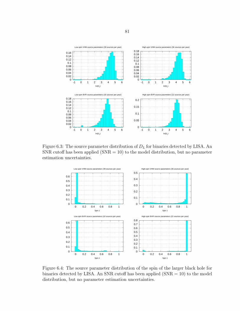
81
00.020.040.060.08
0.10.120.140.16
-1 0 1 2 3 4 5 6ln(DL)
Low-spin VHM source parameters (39 sources per year)
00.020.040.060.08
0.10.120.140.160.18
-1 0 1 2 3 4 5 6ln(DL)
High-spin VHM source parameters (36 sources per year)
00.020.040.060.08
0.10.120.140.160.18
-1 0 1 2 3 4 5 6ln(DL)
Low-spin BVR source parameters (18 sources per year)
0
0.05
0.1
0.15
0.2
-1 0 1 2 3 4 5 6ln(DL)
High-spin BVR source parameters (22 sources per year)
Figure 6.3: The source parameter distribution ofDL for binaries detected by LISA. AnSNR cutoff has been applied (SNR = 10) to the model distribution, but no parameterestimation uncertainties.
0
0.1
0.2
0.3
0.4
0.5
0.6
0 0.2 0.4 0.6 0.8 1Spin 1
Low-spin VHM source parameters (39 sources per year)
0
0.1
0.2
0.3
0.4
0.5
0 0.2 0.4 0.6 0.8 1Spin 1
High-spin VHM source parameters (36 sources per year)
0
0.1
0.2
0.3
0.4
0.5
0.6
0 0.2 0.4 0.6 0.8 1Spin 1
Low-spin BVR source parameters (18 sources per year)
0
0.1
0.2
0.3
0.4
0.5
0.6
0.7
0.8
0 0.2 0.4 0.6 0.8 1Spin 1
High-spin BVR source parameters (22 sources per year)
Figure 6.4: The source parameter distribution of the spin of the larger black hole forbinaries detected by LISA. An SNR cutoff has been applied (SNR = 10) to the modeldistribution, but no parameter estimation uncertainties.
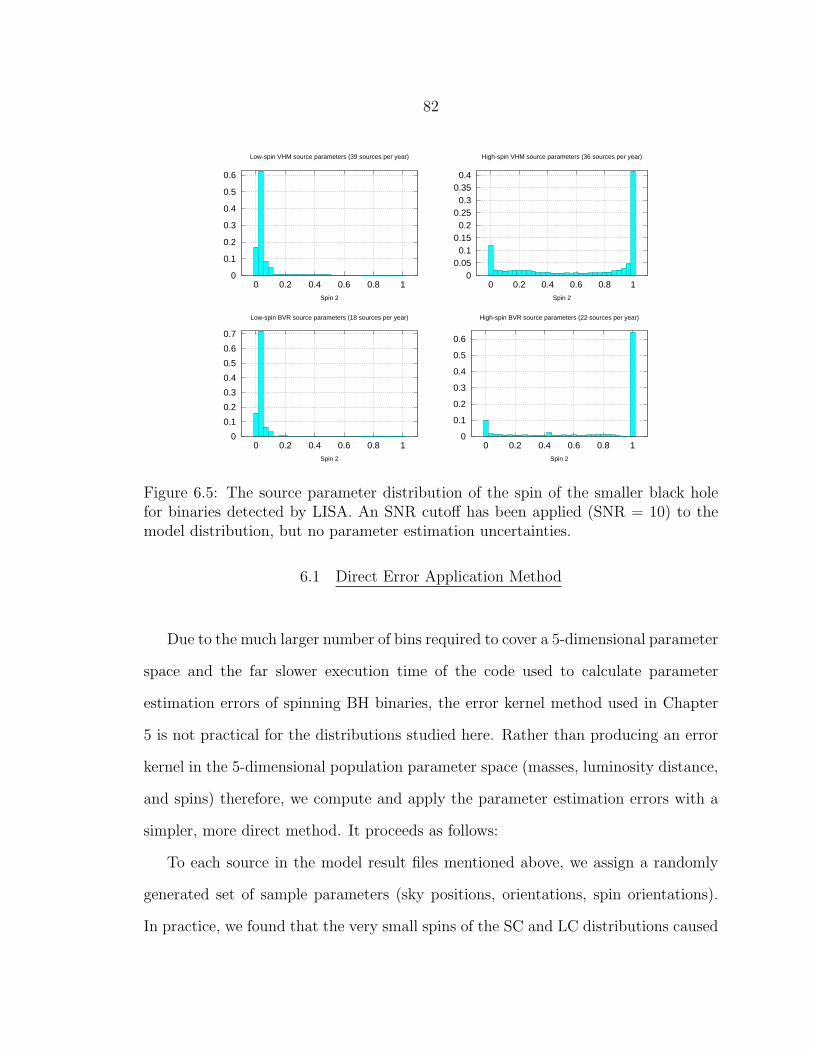
82
0
0.1
0.2
0.3
0.4
0.5
0.6
0 0.2 0.4 0.6 0.8 1Spin 2
Low-spin VHM source parameters (39 sources per year)
00.05
0.10.15
0.20.25
0.30.35
0.4
0 0.2 0.4 0.6 0.8 1Spin 2
High-spin VHM source parameters (36 sources per year)
0
0.1
0.2
0.3
0.4
0.5
0.6
0.7
0 0.2 0.4 0.6 0.8 1Spin 2
Low-spin BVR source parameters (18 sources per year)
0
0.1
0.2
0.3
0.4
0.5
0.6
0 0.2 0.4 0.6 0.8 1Spin 2
High-spin BVR source parameters (22 sources per year)
Figure 6.5: The source parameter distribution of the spin of the smaller black holefor binaries detected by LISA. An SNR cutoff has been applied (SNR = 10) to themodel distribution, but no parameter estimation uncertainties.
6.1 Direct Error Application Method
Due to the much larger number of bins required to cover a 5-dimensional parameter
space and the far slower execution time of the code used to calculate parameter
estimation errors of spinning BH binaries, the error kernel method used in Chapter
5 is not practical for the distributions studied here. Rather than producing an error
kernel in the 5-dimensional population parameter space (masses, luminosity distance,
and spins) therefore, we compute and apply the parameter estimation errors with a
simpler, more direct method. It proceeds as follows:
To each source in the model result files mentioned above, we assign a randomly
generated set of sample parameters (sky positions, orientations, spin orientations).
In practice, we found that the very small spins of the SC and LC distributions caused
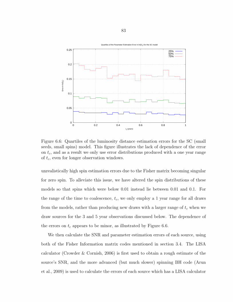
83
0
0.05
0.1
0.15
0.2
0.25
0 0.2 0.4 0.6 0.8 1
Err
or in
ln(D
L)
tc (years)
Quartiles of the Parameter Estimation Error in ln(DL) for the SC model
25%50%75%
Figure 6.6: Quartiles of the luminosity distance estimation errors for the SC (smallseeds, small spins) model. This figure illustrates the lack of dependence of the erroron tc, and as a result we only use error distributions produced with a one year rangeof tc, even for longer observation windows.
unrealistically high spin estimation errors due to the Fisher matrix becoming singular
for zero spin. To alleviate this issue, we have altered the spin distributions of these
models so that spins which were below 0.01 instead lie between 0.01 and 0.1. For
the range of the time to coalescence, tc, we only employ a 1 year range for all draws
from the models, rather than producing new draws with a larger range of tc when we
draw sources for the 3 and 5 year observations discussed below. The dependence of
the errors on tc appears to be minor, as illustrated by Figure 6.6.
We then calculate the SNR and parameter estimation errors of each source, using
both of the Fisher Information matrix codes mentioned in section 3.4. The LISA
calculator (Crowder & Cornish, 2006) is first used to obtain a rough estimate of the
source’s SNR, and the more advanced (but much slower) spinning BH code (Arun
et al., 2009) is used to calculate the errors of each source which has a LISA calculator
84
SNR ≥ 5. The LISA calculator used a galactic foreground confusion noise estimate
from Timpano et al. (2006), while the spinning BHB code used the instrument and
confusion noise model listed in section 4.2 of Arun et al. (2009).
We then store the source parameters, SNRs, and parameter estimation uncertain-
ties (i.e., the a priori standard deviations in the estimated parameters for that set of
source parameters) to disk. Thus, for each of the model result files mentioned above,
we have a corresponding file that lists a full set of binary parameters (including ran-
domly generated sample parameters), binary SNRs, and parameter estimation errors
for every source in the model result file. For each of the low-mass seed models (SC
and SE), there are ≈ 150000 sources, while the high mass seed models have ≈ 40000
sources.
Next, we generate a model predicted realization of the set of sources occurring
during some observation window ∆tobs. We run through each source occurring in the
model’s result files, performing a Bernoulli trial with probability of success given by
equation 6.1 to determine whether that source will occur in the realization. For each
of those sources, we look up its previously calculated parameter estimation errors and
draw from the corresponding gaussian distributions1. This produces a realization of
the model predicted best-fit parameters, as estimated by LISA, for sources occurring
within the observation window.
We then calculate these sets of estimated parameters for a pair of population
models, and compare them using the statistical tests discussed in Chapter 4 to see
whether or not there is a statistically significant difference between them. We re-
1If resulting parameters fall outside of the possible ranges of these parameters (e.g., the spin
parameters lie between 0 and 1, by definition), the parameters are wrapped around so that they
remain within the range. We also add a small 10−3 Gaussian variation to the source parameters, to
avoid issues with the model comparison caused by sources grouped at a single parameter value.
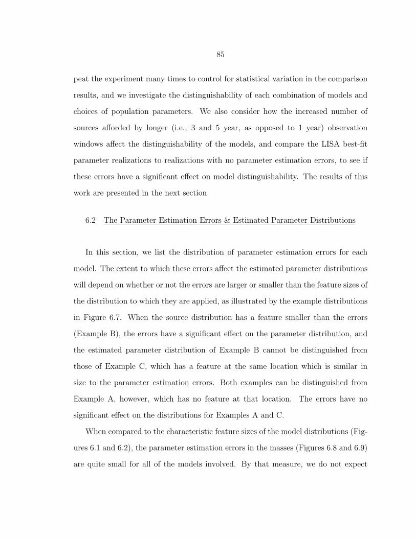
85
peat the experiment many times to control for statistical variation in the comparison
results, and we investigate the distinguishability of each combination of models and
choices of population parameters. We also consider how the increased number of
sources afforded by longer (i.e., 3 and 5 year, as opposed to 1 year) observation
windows affect the distinguishability of the models, and compare the LISA best-fit
parameter realizations to realizations with no parameter estimation errors, to see if
these errors have a significant effect on model distinguishability. The results of this
work are presented in the next section.
6.2 The Parameter Estimation Errors & Estimated Parameter Distributions
In this section, we list the distribution of parameter estimation errors for each
model. The extent to which these errors affect the estimated parameter distributions
will depend on whether or not the errors are larger or smaller than the feature sizes of
the distribution to which they are applied, as illustrated by the example distributions
in Figure 6.7. When the source distribution has a feature smaller than the errors
(Example B), the errors have a significant effect on the parameter distribution, and
the estimated parameter distribution of Example B cannot be distinguished from
those of Example C, which has a feature at the same location which is similar in
size to the parameter estimation errors. Both examples can be distinguished from
Example A, however, which has no feature at that location. The errors have no
significant effect on the distributions for Examples A and C.
When compared to the characteristic feature sizes of the model distributions (Fig-
ures 6.1 and 6.2), the parameter estimation errors in the masses (Figures 6.8 and 6.9)
are quite small for all of the models involved. By that measure, we do not expect
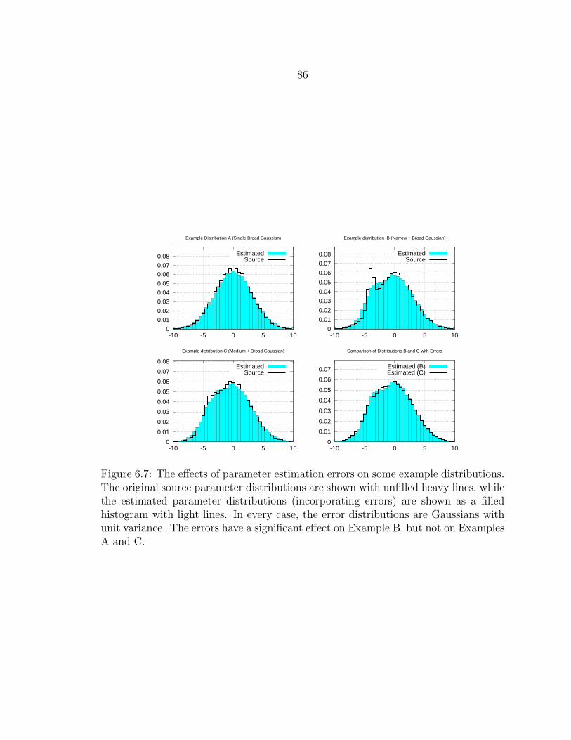
86
0
0.010.02
0.030.04
0.05
0.060.07
0.08
-10 -5 0 5 10
Example Distribution A (Single Broad Gaussian)
EstimatedSource
0
0.01
0.02
0.03
0.04
0.05
0.06
0.07
0.08
-10 -5 0 5 10
Example distribution B (Narrow + Broad Gaussian)
EstimatedSource
0
0.01
0.02
0.03
0.04
0.05
0.06
0.07
0.08
-10 -5 0 5 10
Example distribution C (Medium + Broad Gaussian)
EstimatedSource
0
0.01
0.02
0.03
0.04
0.05
0.06
0.07
-10 -5 0 5 10
Comparison of Distributions B and C with Errors
Estimated (B)Estimated (C)
Figure 6.7: The effects of parameter estimation errors on some example distributions.The original source parameter distributions are shown with unfilled heavy lines, whilethe estimated parameter distributions (incorporating errors) are shown as a filledhistogram with light lines. In every case, the error distributions are Gaussians withunit variance. The errors have a significant effect on Example B, but not on ExamplesA and C.
87
that the parameter estimation errors in the (redshifted) masses to have a significant
effect on LISA’s ability to distinguish between the models.
The luminosity distance errors (Figure 6.10), on the other hand, are somewhat
large compared to the characteristic feature sizes of the models (Figure 6.3), so they
may have an effect on the model distinguishability.
The spin errors are also both large compared to the model feature sizes, but it is
less certain how meaningful the result is in this case. In the case of the high-spin
models, the spin distributions of the sources (Figures 6.4 and 6.5) are extremely tightly
clustered (most of the spins parameters of the larger BH are equal to 0.9982), so that
even though the spin errors (Figures 6.11 and 6.12) are quite small, the parameter
distribution cannot be constrained as tightly as the model’s predicted distribution.
For the low-spin parameters, the parameter estimation errors are unrealistically high,
due to the linear assumptions of the Fisher information matrix approach, and the
actual parameters may be better constrained due to higher order corrections to the
likelihood surface. The large size of the error in spin 2 (i.e., χ2) is not surprising
when we remember that the spin angular momentum of a black hole is given by χm2
(mentioned in section 3.5) and typical mass ratios are ∼ 0.1, so that spin angular
momentum of the smaller BH is only a small fraction of the angular momentum of
the system (recall that χ ≤ 1).
The sizes of these errors are summarized in Table 6.2, which shows the third
quartile parameter estimation error for each combination of model and parameter.
For instance, the entry in the ‘SC’ column and the ‘lnDL’ row shows that 3/4, or
75% of the parameter estimation errors in lnDL for the small seed, chaotic accretion
model are distributed with a standard deviation of 0.168 or less
2Uses an estimated maximum from Thorne (1974)
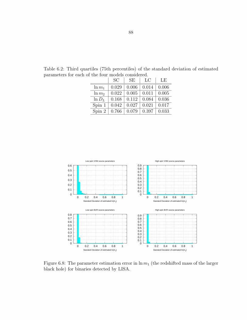
88
Table 6.2: Third quartiles (75th percentiles) of the standard deviation of estimatedparameters for each of the four models considered.
SC SE LC LE
lnm1 0.029 0.006 0.014 0.006lnm2 0.022 0.005 0.011 0.005lnDL 0.168 0.112 0.084 0.036Spin 1 0.042 0.027 0.021 0.017Spin 2 0.766 0.079 0.397 0.033
0
0.1
0.2
0.3
0.4
0.5
0.6
0 0.2 0.4 0.6 0.8 1Standard Deviation of estimated ln(m1)
Low-spin VHM source parameters
00.10.20.30.40.50.60.70.80.9
0 0.2 0.4 0.6 0.8 1Standard Deviation of estimated ln(m1)
High-spin VHM source parameters
00.10.20.30.40.50.60.70.8
0 0.2 0.4 0.6 0.8 1Standard Deviation of estimated ln(m1)
Low-spin BVR source parameters
00.10.20.30.40.50.60.70.80.9
0 0.2 0.4 0.6 0.8 1Standard Deviation of estimated ln(m1)
High-spin BVR source parameters
Figure 6.8: The parameter estimation error in lnm1 (the redshifted mass of the largerblack hole) for binaries detected by LISA.
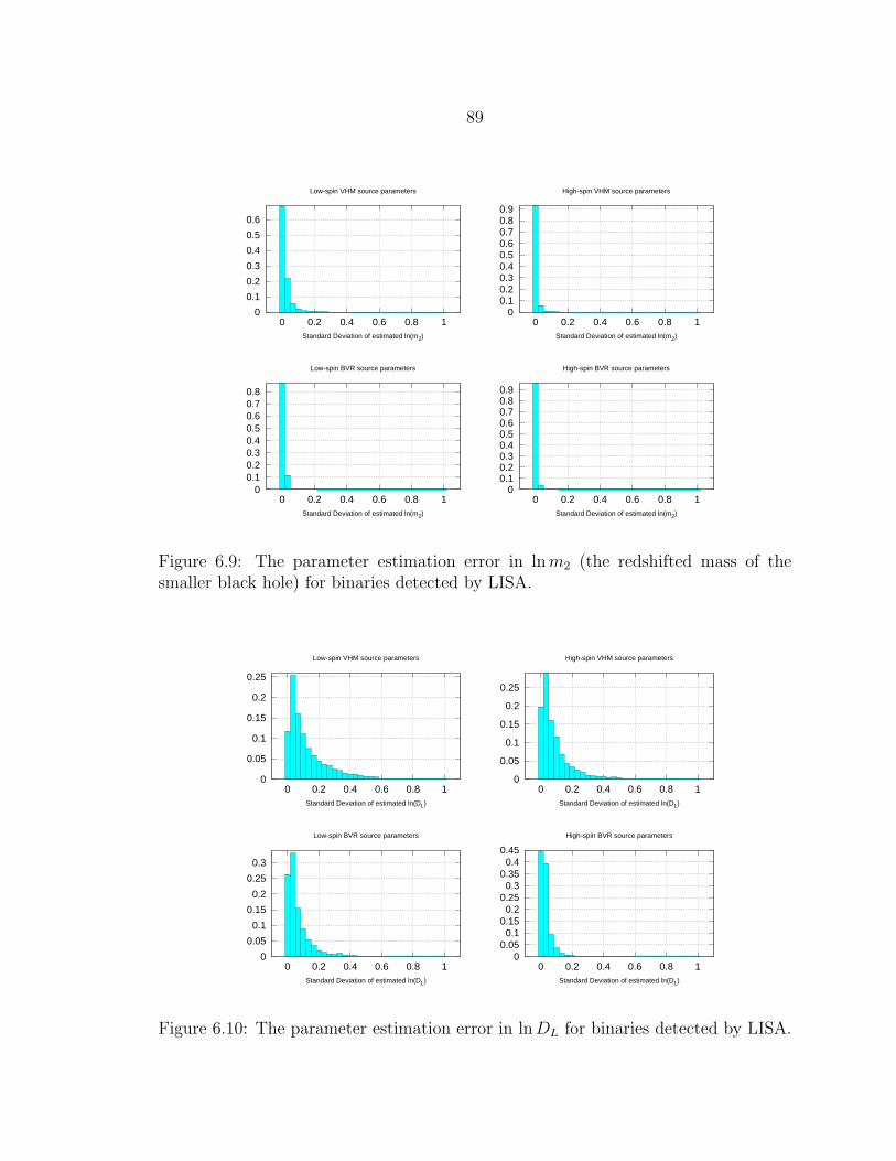
89
0
0.1
0.2
0.3
0.4
0.5
0.6
0 0.2 0.4 0.6 0.8 1Standard Deviation of estimated ln(m2)
Low-spin VHM source parameters
00.10.20.30.40.50.60.70.80.9
0 0.2 0.4 0.6 0.8 1Standard Deviation of estimated ln(m2)
High-spin VHM source parameters
00.10.20.30.40.50.60.70.8
0 0.2 0.4 0.6 0.8 1Standard Deviation of estimated ln(m2)
Low-spin BVR source parameters
00.10.20.30.40.50.60.70.80.9
0 0.2 0.4 0.6 0.8 1Standard Deviation of estimated ln(m2)
High-spin BVR source parameters
Figure 6.9: The parameter estimation error in lnm2 (the redshifted mass of thesmaller black hole) for binaries detected by LISA.
0
0.05
0.1
0.15
0.2
0.25
0 0.2 0.4 0.6 0.8 1Standard Deviation of estimated ln(DL)
Low-spin VHM source parameters
0
0.05
0.1
0.15
0.2
0.25
0 0.2 0.4 0.6 0.8 1Standard Deviation of estimated ln(DL)
High-spin VHM source parameters
0
0.05
0.1
0.15
0.2
0.25
0.3
0 0.2 0.4 0.6 0.8 1Standard Deviation of estimated ln(DL)
Low-spin BVR source parameters
00.05
0.10.15
0.20.25
0.30.35
0.40.45
0 0.2 0.4 0.6 0.8 1Standard Deviation of estimated ln(DL)
High-spin BVR source parameters
Figure 6.10: The parameter estimation error in lnDL for binaries detected by LISA.
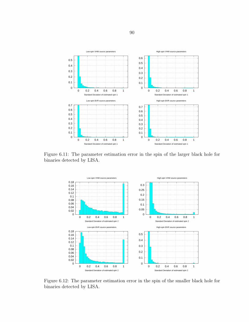
90
0
0.1
0.2
0.3
0.4
0.5
0 0.2 0.4 0.6 0.8 1Standard Deviation of estimated spin 1
Low-spin VHM source parameters
0
0.1
0.2
0.3
0.4
0.5
0.6
0 0.2 0.4 0.6 0.8 1Standard Deviation of estimated spin 1
High-spin VHM source parameters
0
0.1
0.2
0.3
0.4
0.5
0.6
0.7
0 0.2 0.4 0.6 0.8 1Standard Deviation of estimated spin 1
Low-spin BVR source parameters
0
0.1
0.2
0.3
0.4
0.5
0.6
0.7
0 0.2 0.4 0.6 0.8 1Standard Deviation of estimated spin 1
High-spin BVR source parameters
Figure 6.11: The parameter estimation error in the spin of the larger black hole forbinaries detected by LISA.
00.020.040.060.08
0.10.120.140.160.18
0 0.2 0.4 0.6 0.8 1Standard Deviation of estimated spin 2
Low-spin VHM source parameters
0
0.05
0.1
0.15
0.2
0.25
0.3
0 0.2 0.4 0.6 0.8 1Standard Deviation of estimated spin 2
High-spin VHM source parameters
00.020.040.060.08
0.10.120.140.160.18
0 0.2 0.4 0.6 0.8 1Standard Deviation of estimated spin 2
Low-spin BVR source parameters
0
0.1
0.2
0.3
0.4
0.5
0 0.2 0.4 0.6 0.8 1Standard Deviation of estimated spin 2
High-spin BVR source parameters
Figure 6.12: The parameter estimation error in the spin of the smaller black hole forbinaries detected by LISA.
91
Figures 6.13 through 6.17 show the distribution of best-fit parameters which are
obtained when random estimated parameters are drawn from the distribution of each
source’s parameter estimation errors, as described in section 6.1. Each plot also shows,
for comparison, the corresponding source parameter distributions (i.e., Figures 6.1
through 6.5).
As can be seen from the figures, the parameter estimation errors have no significant
effect on the distribution of mass variables. The DL estimation errors, on the other
hand, do have some effect on the distribution of the luminosity distance in the case
of the low spin VHM model (the ‘SE’ model), and a smaller effect on the higher
spin VHM model. The luminosity distance errors do not appear to have a significant
effect on the parameters of the two BVR models (LE and LC), which is unsurprising
given the larger masses and closer distances of those sources. For the low-spin models
(SC and LC), the parameter estimation errors lead to a very significant difference
in the spin distribution of the smaller BH, and a somewhat significant difference in
the spin of the larger BH. For the high-spin models (SE and LE), the effects of the
spin determination errors are less significant, although they still have an effect on
the parameter distribution due to the model’s tight clustering around a spin of 0.998
(also mentioned above).
6.3 Model Comparison Results; 1 and 2 Dimensions
This section reports the results of comparisons between each of the models using
the tests developed in Chapter 4. For each pair of models and model parameters,
we have made 5000 comparisons as described in section 6.1. We quantify the degree
of distinguishability of the models by the fraction of comparisons which resulted in
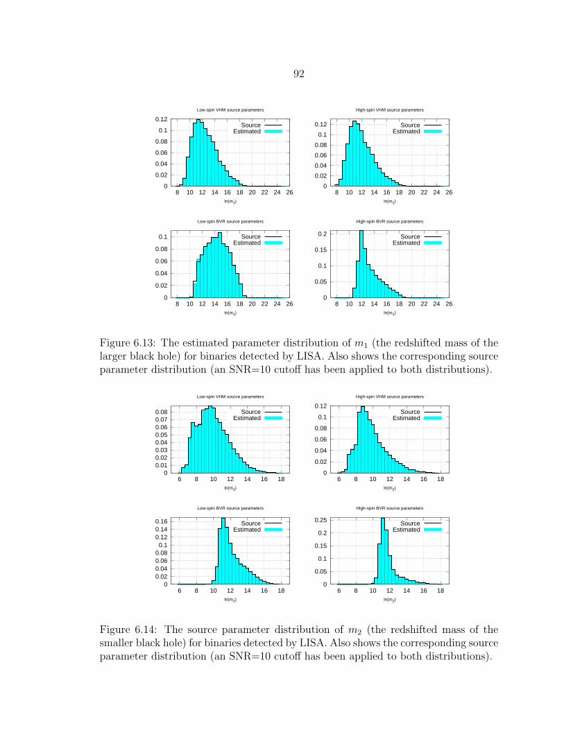
92
0
0.02
0.04
0.06
0.08
0.1
0.12
8 10 12 14 16 18 20 22 24 26ln(m1)
Low-spin VHM source parameters
SourceEstimated
0
0.02
0.04
0.06
0.08
0.1
0.12
8 10 12 14 16 18 20 22 24 26ln(m1)
High-spin VHM source parameters
SourceEstimated
0
0.02
0.04
0.06
0.08
0.1
8 10 12 14 16 18 20 22 24 26ln(m1)
Low-spin BVR source parameters
SourceEstimated
0
0.05
0.1
0.15
0.2
8 10 12 14 16 18 20 22 24 26ln(m1)
High-spin BVR source parameters
SourceEstimated
Figure 6.13: The estimated parameter distribution of m1 (the redshifted mass of thelarger black hole) for binaries detected by LISA. Also shows the corresponding sourceparameter distribution (an SNR=10 cutoff has been applied to both distributions).
00.010.020.030.040.050.060.070.08
6 8 10 12 14 16 18ln(m2)
Low-spin VHM source parameters
SourceEstimated
0
0.02
0.04
0.06
0.08
0.1
0.12
6 8 10 12 14 16 18ln(m2)
High-spin VHM source parameters
SourceEstimated
00.020.040.060.08
0.10.120.140.16
6 8 10 12 14 16 18ln(m2)
Low-spin BVR source parameters
SourceEstimated
0
0.05
0.1
0.15
0.2
0.25
6 8 10 12 14 16 18ln(m2)
High-spin BVR source parameters
SourceEstimated
Figure 6.14: The source parameter distribution of m2 (the redshifted mass of thesmaller black hole) for binaries detected by LISA. Also shows the corresponding sourceparameter distribution (an SNR=10 cutoff has been applied to both distributions).
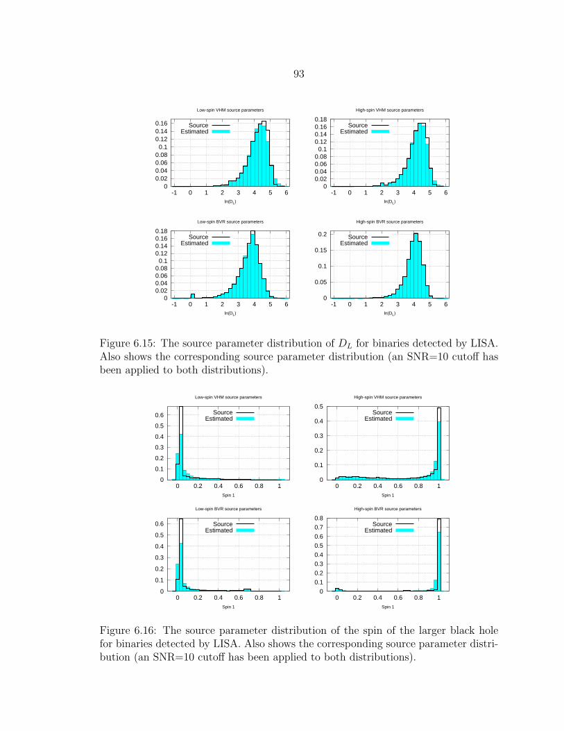
93
00.020.040.060.08
0.10.120.140.16
-1 0 1 2 3 4 5 6ln(DL)
Low-spin VHM source parameters
SourceEstimated
00.020.040.060.08
0.10.120.140.160.18
-1 0 1 2 3 4 5 6ln(DL)
High-spin VHM source parameters
SourceEstimated
00.020.040.060.08
0.10.120.140.160.18
-1 0 1 2 3 4 5 6ln(DL)
Low-spin BVR source parameters
SourceEstimated
0
0.05
0.1
0.15
0.2
-1 0 1 2 3 4 5 6ln(DL)
High-spin BVR source parameters
SourceEstimated
Figure 6.15: The source parameter distribution of DL for binaries detected by LISA.Also shows the corresponding source parameter distribution (an SNR=10 cutoff hasbeen applied to both distributions).
0
0.1
0.2
0.3
0.4
0.5
0.6
0 0.2 0.4 0.6 0.8 1Spin 1
Low-spin VHM source parameters
SourceEstimated
0
0.1
0.2
0.3
0.4
0.5
0 0.2 0.4 0.6 0.8 1Spin 1
High-spin VHM source parameters
SourceEstimated
0
0.1
0.2
0.3
0.4
0.5
0.6
0 0.2 0.4 0.6 0.8 1Spin 1
Low-spin BVR source parameters
SourceEstimated
0
0.1
0.2
0.3
0.4
0.5
0.6
0.7
0.8
0 0.2 0.4 0.6 0.8 1Spin 1
High-spin BVR source parameters
SourceEstimated
Figure 6.16: The source parameter distribution of the spin of the larger black holefor binaries detected by LISA. Also shows the corresponding source parameter distri-bution (an SNR=10 cutoff has been applied to both distributions).
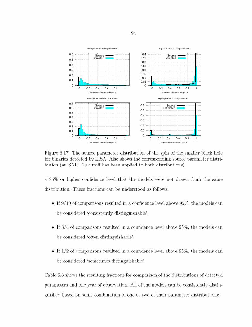
94
0
0.1
0.2
0.3
0.4
0.5
0.6
0 0.2 0.4 0.6 0.8 1Distribution of estimated spin 2
Low-spin VHM source parameters
SourceEstimated
00.05
0.10.15
0.20.25
0.30.35
0.4
0 0.2 0.4 0.6 0.8 1Distribution of estimated spin 2
High-spin VHM source parameters
SourceEstimated
0
0.1
0.2
0.3
0.4
0.5
0.6
0.7
0 0.2 0.4 0.6 0.8 1Distribution of estimated spin 2
Low-spin BVR source parameters
SourceEstimated
0
0.1
0.2
0.3
0.4
0.5
0.6
0 0.2 0.4 0.6 0.8 1Distribution of estimated spin 2
High-spin BVR source parameters
SourceEstimated
Figure 6.17: The source parameter distribution of the spin of the smaller black holefor binaries detected by LISA. Also shows the corresponding source parameter distri-bution (an SNR=10 cutoff has been applied to both distributions).
a 95% or higher confidence level that the models were not drawn from the same
distribution. These fractions can be understood as follows:
• If 9/10 of comparisons resulted in a confidence level above 95%, the models can
be considered ‘consistently distinguishable’.
• If 3/4 of comparisons resulted in a confidence level above 95%, the models can
be considered ‘often distinguishable’.
• If 1/2 of comparisons resulted in a confidence level above 95%, the models can
be considered ‘sometimes distinguishable’.
Table 6.3 shows the resulting fractions for comparison of the distributions of detected
parameters and one year of observation. All of the models can be consistently distin-
guished based on some combination of one or two of their parameter distributions:
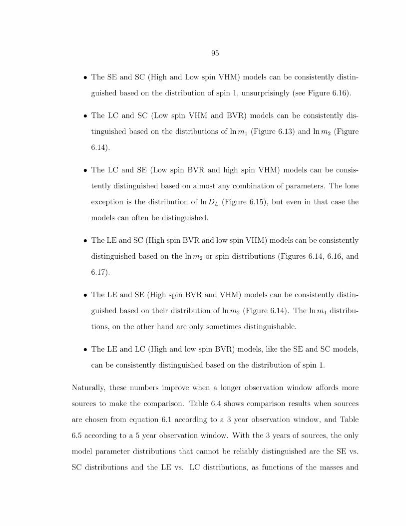
95
• The SE and SC (High and Low spin VHM) models can be consistently distin-
guished based on the distribution of spin 1, unsurprisingly (see Figure 6.16).
• The LC and SC (Low spin VHM and BVR) models can be consistently dis-
tinguished based on the distributions of lnm1 (Figure 6.13) and lnm2 (Figure
6.14).
• The LC and SE (Low spin BVR and high spin VHM) models can be consis-
tently distinguished based on almost any combination of parameters. The lone
exception is the distribution of lnDL (Figure 6.15), but even in that case the
models can often be distinguished.
• The LE and SC (High spin BVR and low spin VHM) models can be consistently
distinguished based on the lnm2 or spin distributions (Figures 6.14, 6.16, and
6.17).
• The LE and SE (High spin BVR and VHM) models can be consistently distin-
guished based on their distribution of lnm2 (Figure 6.14). The lnm1 distribu-
tions, on the other hand are only sometimes distinguishable.
• The LE and LC (High and low spin BVR) models, like the SE and SC models,
can be consistently distinguished based on the distribution of spin 1.
Naturally, these numbers improve when a longer observation window affords more
sources to make the comparison. Table 6.4 shows comparison results when sources
are chosen from equation 6.1 according to a 3 year observation window, and Table
6.5 according to a 5 year observation window. With the 3 years of sources, the only
model parameter distributions that cannot be reliably distinguished are the SE vs.
SC distributions and the LE vs. LC distributions, as functions of the masses and
96
Table 6.3: E statistic Model comparison results for 1 year of observation, showing thefraction of confidence levels which were above 95%. To make the table easier to read,comparisons where 1/2 of the confidence levels were above 95% are marked in lightgray, comparisons where 3/4 were above 95% are marked in medium gray, and thosewhere 9/10 were above 95% are marked in dark gray.
SE vs. SC LC vs. SC LC vs. SE LE vs. SC LE vs. SE LE vs. LClnm1 0.0776 0.918 0.9274 0.566 0.5992 0.163
lnm2 & lnm1 0.086 0.989 0.9926 0.9716 0.9878 0.1982lnm2 0.0618 0.989 0.991 0.9842 0.9948 0.1148
lnDL & lnm1 0.0894 0.9504 0.9532 0.5296 0.5502 0.2964lnDL & lnm2 0.0716 0.9936 0.9946 0.9678 0.9876 0.2376
lnDL 0.0562 0.8956 0.8422 0.5336 0.4366 0.1834Spin 1 & lnm1 1 0.9154 1 1 0.6742 0.9854Spin 1 & lnm2 1 0.9774 1 1 0.9964 0.9758Spin 1 & lnDL 1 0.8912 0.9992 1 0.5204 0.9674
Spin 1 1 0.784 0.9996 1 0.5086 0.9808Spin 2 & lnm1 0.7958 0.9574 0.9982 0.9792 0.6928 0.892Spin 2 & lnm2 0.7882 0.9898 1 0.9992 0.9944 0.8186Spin 2 & lnDL 0.7638 0.9086 0.9696 0.9622 0.5136 0.7682Spin 2 & Spin 1 1 0.836 0.9996 1 0.59 0.9918
Spin 2 0.7674 0.8328 0.9646 0.983 0.494 0.786
DL. The SE and SC distributions of masses and DL, in particular, are not generally
distinguishable. The distributions of lnDL and lnm1 for the LE and LC models, on
the other hand, are often distinguishable. With 5 years worth of sources, the LE and
LC mass and redshift distributions (especially the distribution of lnDL and lnm1)
can be consistently distinguished from each other, but the SE and SC distributions
remain indistinguishable.
Since we are interested as much in the limits of LISA’s ability to distinguish
between the population models as in whether or not LISA will be able to distinguish
between these particular sets of models (which will undoubtedly be superseded with
improved versions by the time LISA is operational), Figures 6.18 and 6.19 show the
distributions of lnDL and lnm1, and of lnDL and lnm2. The plots serve to illustrate
distributions which have varying levels of distinguishability.
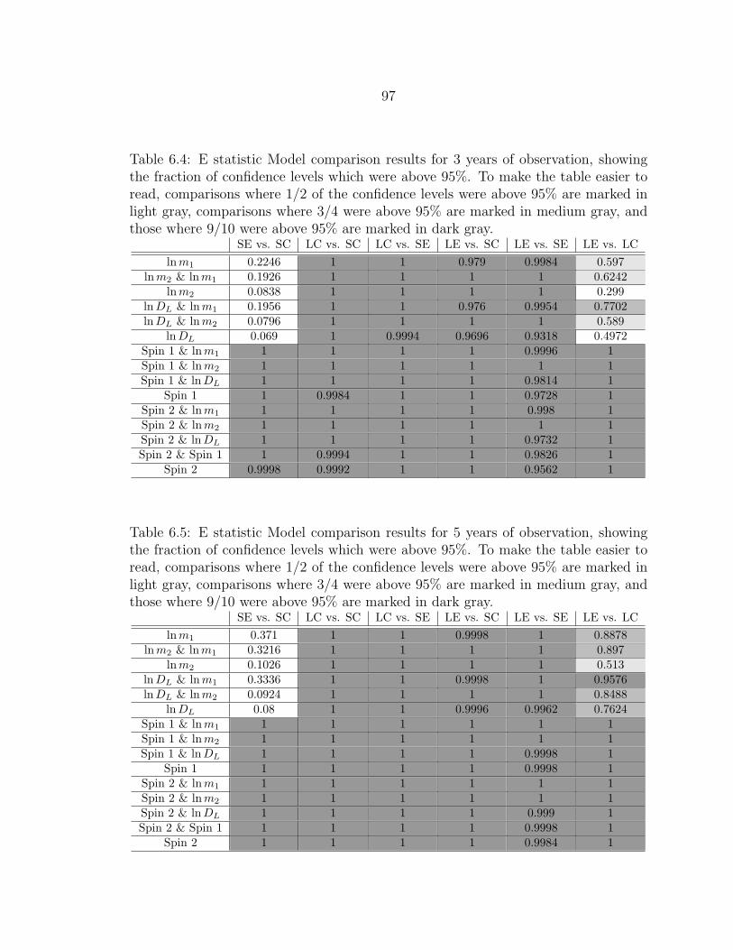
97
Table 6.4: E statistic Model comparison results for 3 years of observation, showingthe fraction of confidence levels which were above 95%. To make the table easier toread, comparisons where 1/2 of the confidence levels were above 95% are marked inlight gray, comparisons where 3/4 were above 95% are marked in medium gray, andthose where 9/10 were above 95% are marked in dark gray.
SE vs. SC LC vs. SC LC vs. SE LE vs. SC LE vs. SE LE vs. LClnm1 0.2246 1 1 0.979 0.9984 0.597
lnm2 & lnm1 0.1926 1 1 1 1 0.6242lnm2 0.0838 1 1 1 1 0.299
lnDL & lnm1 0.1956 1 1 0.976 0.9954 0.7702lnDL & lnm2 0.0796 1 1 1 1 0.589
lnDL 0.069 1 0.9994 0.9696 0.9318 0.4972Spin 1 & lnm1 1 1 1 1 0.9996 1Spin 1 & lnm2 1 1 1 1 1 1Spin 1 & lnDL 1 1 1 1 0.9814 1
Spin 1 1 0.9984 1 1 0.9728 1Spin 2 & lnm1 1 1 1 1 0.998 1Spin 2 & lnm2 1 1 1 1 1 1Spin 2 & lnDL 1 1 1 1 0.9732 1Spin 2 & Spin 1 1 0.9994 1 1 0.9826 1
Spin 2 0.9998 0.9992 1 1 0.9562 1
Table 6.5: E statistic Model comparison results for 5 years of observation, showingthe fraction of confidence levels which were above 95%. To make the table easier toread, comparisons where 1/2 of the confidence levels were above 95% are marked inlight gray, comparisons where 3/4 were above 95% are marked in medium gray, andthose where 9/10 were above 95% are marked in dark gray.
SE vs. SC LC vs. SC LC vs. SE LE vs. SC LE vs. SE LE vs. LClnm1 0.371 1 1 0.9998 1 0.8878
lnm2 & lnm1 0.3216 1 1 1 1 0.897lnm2 0.1026 1 1 1 1 0.513
lnDL & lnm1 0.3336 1 1 0.9998 1 0.9576lnDL & lnm2 0.0924 1 1 1 1 0.8488
lnDL 0.08 1 1 0.9996 0.9962 0.7624Spin 1 & lnm1 1 1 1 1 1 1Spin 1 & lnm2 1 1 1 1 1 1Spin 1 & lnDL 1 1 1 1 0.9998 1
Spin 1 1 1 1 1 0.9998 1Spin 2 & lnm1 1 1 1 1 1 1Spin 2 & lnm2 1 1 1 1 1 1Spin 2 & lnDL 1 1 1 1 0.999 1Spin 2 & Spin 1 1 1 1 1 0.9998 1
Spin 2 1 1 1 1 0.9984 1
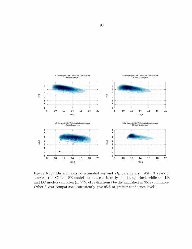
98
ln(D
L)
ln(m1)
SC (Low-spin VHM) Estimated parameters39 events per year
-10123456
8 10 12 14 16 18 20
ln(D
L)
ln(m1)
SE (High-spin VHM) Estimated parameters36 events per year
-10123456
8 10 12 14 16 18 20
ln(D
L)
ln(m1)
LC (Low-spin BVR) Estimated parameters18 events per year
-10123456
8 10 12 14 16 18 20
ln(D
L)
ln(m1)
LE (High-spin BVR) Estimated parameters22 events per year
-10123456
8 10 12 14 16 18 20
Figure 6.18: Distributions of estimated m1 and DL parameters. With 3 years ofsources, the SC and SE models cannot consistently be distinguished, while the LEand LC models can often (in 77% of realizations) be distinguished at 95% confidence.Other 3 year comparisons consistently give 95% or greater confidence levels.
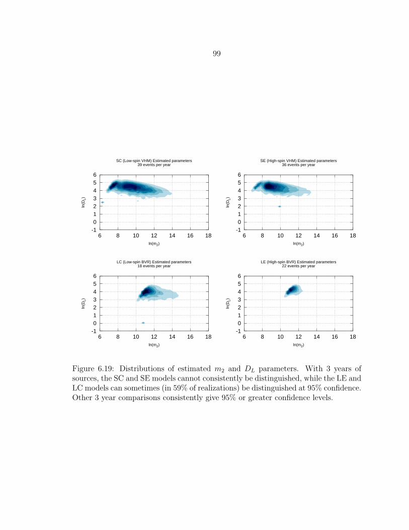
99
ln(D
L)
ln(m2)
SC (Low-spin VHM) Estimated parameters39 events per year
-10123456
6 8 10 12 14 16 18
ln(D
L)
ln(m2)
SE (High-spin VHM) Estimated parameters36 events per year
-10123456
6 8 10 12 14 16 18
ln(D
L)
ln(m2)
LC (Low-spin BVR) Estimated parameters18 events per year
-10123456
6 8 10 12 14 16 18
ln(D
L)
ln(m2)
LE (High-spin BVR) Estimated parameters22 events per year
-10123456
6 8 10 12 14 16 18
Figure 6.19: Distributions of estimated m2 and DL parameters. With 3 years ofsources, the SC and SE models cannot consistently be distinguished, while the LE andLC models can sometimes (in 59% of realizations) be distinguished at 95% confidence.Other 3 year comparisons consistently give 95% or greater confidence levels.
100
6.3.1 Effects of Parameter Estimation Errors on Model Distinguishability
In order to assess the significance of the effects of parameter estimation error
on the distinguishability of the models, we have also performed model comparison
tests with no parameter estimation errors. The results of these tests, for one year
of observations, are shown in Table 6.6. The differences between these model distin-
guishability fractions and those found in Table 6.3 (which incorporate the parameter
estimation errors) are shown in Table 6.7. These differences show how the fraction
of significantly different model realizations decreases when the parameter estimation
errors are applied.
For comparison of the SE and SC models (and to a lesser extent for the LE and LC
models), the parameter estimation errors in the spin of the smaller BH significantly
decrease the fraction of significantly different model realizations, as anticipated in
section 6.2. The parameter estimation errors in DL might be expected to have an
effect on the distinguishability of some of the model parameter distributions, but
it appears that they do not. This is not so surprising when we remember that the
source distributions of DL (Figure 6.3) are fairly smooth on the scale of the parameter
estimation errors in DL (Figure 6.10). The effects of parameter estimation error on
the distributions of the spin of the second BH and on DL can be seen in Figures 6.17
and 6.15, respectively. Other than the distributions of spin 2 and DL, the parameter
estimation errors have no significant effect on the fraction of confidence levels above
95%. Of the distributions considered here, only the spin distributions are sharply
peaked enough (compared to the errors) for the parameter estimation errors to have
a significant effect on model distinguishability.
In some cases, application of the parameter estimation errors causes the confidence
levels to increase slightly. This is due to cases where one of the parameters (e.g., DL)
101
for two models are distributed quite similarly, but the parameter estimation errors
are significantly different between the models, due to one of the other parameters
(such as the spins) affecting the GW signal having very different distributions. Thus,
the source parameter (e.g., DL) distribution can be very similar, while the estimated
parameter distribution can be different (due to a larger spread in the distribution of
the source with larger parameters). This does not mean that it is possible for the
models to be more distinguishable on the whole with errors than without, however,
since we are ignoring the parameter distributions (the spins in this example) that are
very different and concentrating on just one of the parameter dimensions of the model.
When we consider the distinguishability of the models across all of the parameters
which affect the signal, we should find that the models are indeed less distinguishable
when the parameter estimation errors are applied. This is what we see when we
look at Table 6.7: the parameter estimation errors for each of the model comparisons
decreases the fraction of confidence levels above 95% (the positive values in the table)
more frequently than it increases them (the negative values in the table).
6.4 Summary
This work makes use of 4 sets of model simulation results (see also Arun et al.,
2009), each of which uses a different combination of two accretion (‘chaotic’ - low
spins and ‘efficient’ - high spins) and seeding (low mass and high mass) scenarios.
The results are labelled ‘Small Chaotic’ (SC), ‘Small Efficient’ (SE), ‘Large Chaotic’
(LC), and ‘Large Efficient’ (LE). We have applied the LISA parameter estimation
errors and SNR thresholds to each, allowing us to produce realizations of the LISA
estimated parameter distributions predicted by the models. We then compare these
estimated parameter distributions using the 1 and 2-Dimensional variants of the K-S
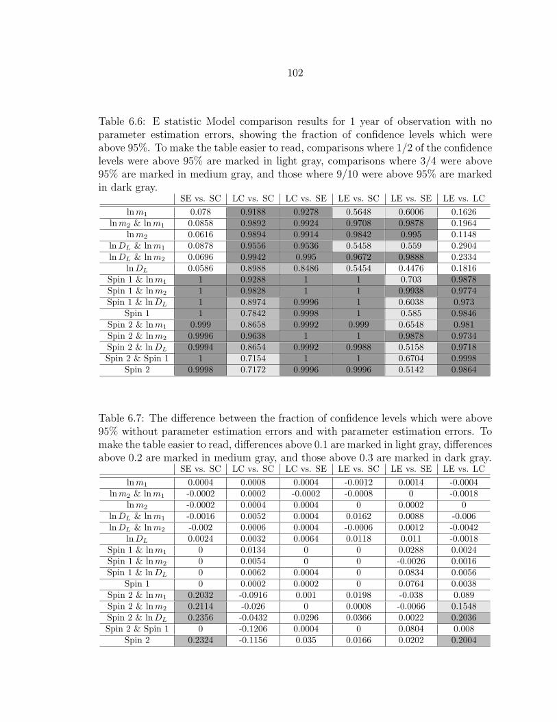
102
Table 6.6: E statistic Model comparison results for 1 year of observation with noparameter estimation errors, showing the fraction of confidence levels which wereabove 95%. To make the table easier to read, comparisons where 1/2 of the confidencelevels were above 95% are marked in light gray, comparisons where 3/4 were above95% are marked in medium gray, and those where 9/10 were above 95% are markedin dark gray.
SE vs. SC LC vs. SC LC vs. SE LE vs. SC LE vs. SE LE vs. LClnm1 0.078 0.9188 0.9278 0.5648 0.6006 0.1626
lnm2 & lnm1 0.0858 0.9892 0.9924 0.9708 0.9878 0.1964lnm2 0.0616 0.9894 0.9914 0.9842 0.995 0.1148
lnDL & lnm1 0.0878 0.9556 0.9536 0.5458 0.559 0.2904lnDL & lnm2 0.0696 0.9942 0.995 0.9672 0.9888 0.2334
lnDL 0.0586 0.8988 0.8486 0.5454 0.4476 0.1816Spin 1 & lnm1 1 0.9288 1 1 0.703 0.9878Spin 1 & lnm2 1 0.9828 1 1 0.9938 0.9774Spin 1 & lnDL 1 0.8974 0.9996 1 0.6038 0.973
Spin 1 1 0.7842 0.9998 1 0.585 0.9846Spin 2 & lnm1 0.999 0.8658 0.9992 0.999 0.6548 0.981Spin 2 & lnm2 0.9996 0.9638 1 1 0.9878 0.9734Spin 2 & lnDL 0.9994 0.8654 0.9992 0.9988 0.5158 0.9718Spin 2 & Spin 1 1 0.7154 1 1 0.6704 0.9998
Spin 2 0.9998 0.7172 0.9996 0.9996 0.5142 0.9864
Table 6.7: The difference between the fraction of confidence levels which were above95% without parameter estimation errors and with parameter estimation errors. Tomake the table easier to read, differences above 0.1 are marked in light gray, differencesabove 0.2 are marked in medium gray, and those above 0.3 are marked in dark gray.
SE vs. SC LC vs. SC LC vs. SE LE vs. SC LE vs. SE LE vs. LClnm1 0.0004 0.0008 0.0004 -0.0012 0.0014 -0.0004
lnm2 & lnm1 -0.0002 0.0002 -0.0002 -0.0008 0 -0.0018lnm2 -0.0002 0.0004 0.0004 0 0.0002 0
lnDL & lnm1 -0.0016 0.0052 0.0004 0.0162 0.0088 -0.006lnDL & lnm2 -0.002 0.0006 0.0004 -0.0006 0.0012 -0.0042
lnDL 0.0024 0.0032 0.0064 0.0118 0.011 -0.0018Spin 1 & lnm1 0 0.0134 0 0 0.0288 0.0024Spin 1 & lnm2 0 0.0054 0 0 -0.0026 0.0016Spin 1 & lnDL 0 0.0062 0.0004 0 0.0834 0.0056
Spin 1 0 0.0002 0.0002 0 0.0764 0.0038Spin 2 & lnm1 0.2032 -0.0916 0.001 0.0198 -0.038 0.089Spin 2 & lnm2 0.2114 -0.026 0 0.0008 -0.0066 0.1548Spin 2 & lnDL 0.2356 -0.0432 0.0296 0.0366 0.0022 0.2036Spin 2 & Spin 1 0 -0.1206 0.0004 0 0.0804 0.008
Spin 2 0.2324 -0.1156 0.035 0.0166 0.0202 0.2004
103
test developed in Chapter 4, investigating how the distinguishability of the models
varies with the choice of parameter compared, the length of the observation window,
and other factors. The results are as follows:
• All of the models compared can be consistently distinguished with a single year
of LISA data, the spin distributions of the chaotic accretion models (SC, LC)
being almost trivially distinguishable from those of the efficient accretion models
(SE, LE).
• The parameter estimation errors in the spin of the smaller BH can have appre-
ciable effects on the distinguishability of the models, while those in the masses
and the spin of the large BH do not. The parameter estimation errors in lnDL
are too small, compared to the rather smooth model lnDL distributions, to have
a significant effect on the model distinguishability.
• The distributions of estimated lnm1 and lnDL for each of the four models illus-
trate which parameter distributions LISA can distinguish with ease, and which
are more difficult to distinguish. For instance, LISA cannot distinguish between
these distributions for the SE vs. SC comparison, but can often distinguish
between them for the LE vs. LC comparison (given 3 years of observation).
The ease with which these models can be distinguished demonstrate the promise of
LISA, and point the way forward for MBH population modelers and model comparison
testing. It is clear from these results that LISA is uniquely suited to examining and
constraining the distribution of the cosmological MBH population. Moreover, since
these models are so readily distinguished, it is clear that LISA will also be able to
discriminate between significantly more subtle variations between the populations.
104
Note that the model comparisons performed here made use only of the estimated,
or best-fit, parameters associated with sources found in a realization of the LISA data
stream. They do not consider the posterior distribution of likely source parameters
associated with each binary whose presence is inferred from a realization of the LISA
data stream.In reality, we will be able to determine from the LISA waveform that some
sources will have better signals (e.g., those with a higher SNR or longer observation
time) than others, and the range of binary parameters which could have given rise to
these detected events will be more tightly constrained. Thus, some sources will have
a larger contribution to our state of knowledge about the population models than
others. In order to take these varying contributions into account, Bayesian model
selection methods should be employed, as discussed in Chapter 8.
105
CHAPTER 7
CONCLUSION
In this work, we have applied the Laser Interferometer (LISA) parameter estima-
tion errors to the populations of Massive Black Holes predicted by various models,
and compared the distinguishability of the resulting distributions of parameters. We
consider how the distinguishability of the models varies depending on the choice of
parameters compared, the time of observation, and whether or not the parameter esti-
mation errors are applied. Our objective is to investigate LISA’s ability to distinguish
between population models; for instance, how dissimilar from the actual population
does a model population need to be before it can be distinguished based on the LISA
data?
Chapter 1 introduces the problem and gives an outline of the dissertation.
Chapter 2 reviews the state of the astrophysics behind the population models,
and the implementation of the models. We review various important aspects of
the models, such as the seeding and accretion prescriptions. We describe the semi-
analytical approach which produced the model simulation results used in this work
(specifically, we use simulations based on Volonteri et al., 2003), and mention which
seeding (Volonteri et al., 2003; Begelman et al., 2006) and accretion (Thorne, 1974;
King & Pringle, 2006) prescriptions are used in the simulations. We also review the
astrophysical processes being modeled to which we might expect LISA to be sensitive.
Chapter 3 reviews Gravitational Wave (GW) production and detection. We begin
by describing the promise of GW detection, discussing current and future detectors.
Next, beginning with Einstein’s equation, we describe how GWs are produced, and
how they can be detected. We then specialize to the case of LISA, introducing the
response of LISA and LISA signal-to-noise (SNR) calculations. We then show the
106
derivation of the Fisher Information Matrix (FIM), which we use to approximate the
parameter estimation errors of sources extracted from the LISA data stream. Lastly,
we describe each of the parameters which define a black hole binary, dividing them
into ‘population’ parameters, whose distribution depends on the population model,
and ‘sample’ parameters, which have the same distribution for all population models.
In Chapter 4, we introduce the modified versions of the Kolmogorov-Smirnov (K-
S) D statistic, which we call the ‘E statistic’, used to quantify the degree of difference
between the model parameter distributions. We illustrate the calculation of these
statistics, describe how their confidence levels are calculated, and demonstrate that
the distribution of the E statistic in the case of the null hypothesis is essentially
independent of the distribution of the data sets being compared.
Chapter 5 illustrated the computation of an error kernel, K(λi, λi), which can be
applied directly to model coalescence rates, producing a new set of predicted detection
rates as functions of the best-fitting, ‘detected’, parameter values. The error kernels
allow visualization of the distribution of parameter estimation errors for a particular
source predicted by a model, and can be constructed without reference to any single
model. We produced estimated detection rates for several populations drawn from
Sesana et al. (2007), and compared them with each other using the modified version
of the one dimensional Kolmogorov-Smirnov (K-S) test discussed in Chapter 4. Our
tests found the model predictions to be statistically different, indicating that LISA
will have appreciable model-discriminating power and is likely to finally resolve the
question of the origin of MBHs.
In Chapter 6, we apply the parameter estimation errors directly to four sets of
simulation results obtained from Dr. Marta Volonteri (also used in Arun et al., 2009).
The parameter estimation errors are applied by generating a random set of population
parameters for each source which occurs in a realization, calculating the errors corre-
107
sponding to that source, and generating the source’s estimated parameters from the
corresponding Gaussian distribution. We then compare the resulting distributions of
estimated parameters using the tests developed in Chapter 4. We found that each of
the models can be distinguished based on 1 year of LISA observations, investigated
the effects of parameter estimation errors on the distinguishability of the models, and
examined which parameter distributions were indistinguishable, which were easily
distinguishable, and which were difficult to distinguish.
In summary, we find that LISA can discriminate between each of the models
studied here, and that it possesses a strong ability to distinguish between various
scenarios for the origins of SMBHs. In particular, the seeding and feedback formation
scenarios here are readily distinguishable on the basis of LISA observations, but would
be very difficult to distinguish based on electromagnetic observations. Comparison of
the LC vs. LE and SE vs. SC models (see Figures 6.18 and 6.19) gives a good example
of estimated mass and luminosity distance distributions which are challenging to
distinguish (LC vs. LE) and indistinguishable (SC vs. SE).
108
CHAPTER 8
FUTURE WORK
The natural direction for future research on this topic will be to move beyond the
Fisher Information Matrix error estimates and the frequentist K-S tests, and employ
Bayesian parameter uncertainty estimates and model selection methods:
• Produce improved, more accurate parameter uncertainty estimates, particularly
Bayesian estimates of source posterior probability distributions (e.g., Littenberg
& Cornish, 2009).
• Develop Bayesian population model comparison tests which are sensitive to the
full dimensionality of the population parameter space (binary masses, distance
and spins). These tests would be used in conjunction with the Bayesian source
posterior distributions mentioned above.
• Investigate the uncertainty in the models, or their sensitivity to variation in the
assumptions they employ. This will involve interdisciplinary collaboration with
the researchers who have developed the population models.
The objective would be to produce a statistically sound, end-to-end study of the
strength of the LISA data stream’s constraints on the astrophysical processes involved
in cosmological massive black hole formation and evolution. While LISA’s probable
discovery of a significant number of gravitational wave sources will be exciting in
its own right, this work will bridge the gap between gravitational wave detection
research and MBH population modeling, exploring how to put LISA’s discoveries to
use in investigating the origins and evolution of cosmological massive black holes, an
important question in contemporary astrophysics. Many of these techniques could
also be applied to other classes of error analysis and model comparison problems.
109
Bibliography
Abbott, B. P., Abbott, R., Adhikari, R., Ajith, P., Allen, B., Allen, G., Amin, R. S.,Anderson, S. B., Anderson, W. G., Arain, M. A., Araya, M., Armandula, H.,Armor, P., Aso, Y., Aston, S., Aufmuth, P., Aulbert, C., Babak, S., Baker, P.,Ballmer, S., Barker, C., Barker, D., Barr, B., Barriga, P., Barsotti, L., Barton,M. A., & Bartos, I. 2009, Phys. Rev. D, 80, 047101
Apostolatos, T. A., Cutler, C., Sussman, G. J., & Thorne, K. S. 1994, Phys. Rev. D,49, 6274
Arun, K. G., Babak, S., Berti, E., Cornish, N., Cutler, C., Gair, J., Hughes, S. A.,Iyer, B. R., Lang, R. N., Mandel, I., Porter, E. K., Sathyaprakash, B. S., Sinha, S.,Sintes, A. M., Trias, M., Van Den Broeck, C., & Volonteri, M. 2009, Classical andQuantum Gravity, 26, 094027
Baker, J. G., Centrella, J., Choi, D., Koppitz, M., & van Meter, J. 2006, Phys. Rev. D,73, 104002
Becker, R. H., Fan, X., White, R. L., Strauss, M. A., Narayanan, V. K., Lupton,R. H., Gunn, J. E., Annis, J., Bahcall, N. A., Brinkmann, J., Connolly, A. J.,Csabai, I., Czarapata, P. C., Doi, M., Heckman, T. M., Hennessy, G. S., Ivezic,Z., Knapp, G. R., Lamb, D. Q., McKay, T. A., Munn, J. A., Nash, T., Nichol, R.,Pier, J. R., Richards, G. T., Schneider, D. P., Stoughton, C., Szalay, A. S., Thakar,A. R., & York, D. G. 2001, AJ, 122, 2850
Begelman, M. C., Volonteri, M., & Rees, M. J. 2006, MNRAS, 370, 289
Berti, E. & Volonteri, M. 2008, ApJ, 684, 822
Blanchet, L. 2006, Living Reviews in Relativity, 9, 4
Bond, J. R., Cole, S., Efstathiou, G., & Kaiser, N. 1991, ApJ, 379, 440
Bromm, V. & Loeb, A. 2003, ApJ, 596, 34
Campanelli, M., Lousto, C., Zlochower, Y., & Merritt, D. 2007, ApJ, 659, L5
Cole, S., Lacey, C. G., Baugh, C. M., & Frenk, C. S. 2000, MNRAS, 319, 168
Cornish, N. J. 2009, Phys. Rev. D, 80, 087101
Crowder, J. & Cornish, N. 2006, LISA Calculator, http://www.physics.montana.edu/lisa/lisacalculator/
Crowder, J. O. 2006, PhD thesis, Montana State University, United States – Montana
Cutler, C. & Flanagan, E. E. 1994, Phys. Rev. D, 49, 2658
110
Danzmann, K. & Rudiger, A. 2003, Classical and Quantum Gravity, 20, 1
Ebisuzaki, T., Makino, J., Tsuru, T. G., Funato, Y., Portegies Zwart, S., Hut, P.,McMillan, S., Matsushita, S., Matsumoto, H., & Kawabe, R. 2001, ApJ, 562, L19
Efstathiou, G., Frenk, C. S., White, S. D. M., & Davis, M. 1988, MNRAS, 235, 715
Eke, V. R., Navarro, J. F., & Frenk, C. S. 1998, ApJ, 503, 569
Fan, X., Narayanan, V. K., Lupton, R. H., Strauss, M. A., Knapp, G. R., Becker,R. H., White, R. L., Pentericci, L., Leggett, S. K., Haiman, Z., Gunn, J. E., Ivezic,Z., Schneider, D. P., Anderson, S. F., Brinkmann, J., Bahcall, N. A., Connolly,A. J., Csabai, I., Doi, M., Fukugita, M., Geballe, T., Grebel, E. K., Harbeck, D.,Hennessy, G., Lamb, D. Q., Miknaitis, G., Munn, J. A., Nichol, R., Okamura, S.,Pier, J. x., Prada, F., Richards, G. T., Szalay, A., & York, D. G. 2001, AJ, 122,2833
Fasano, G. & Franceschini, A. 1987, MNRAS, 225, 155
Ferrarese, L. & Merritt, D. 2000, ApJ, 539, L9
Finn, L. S. 2009, Phys. Rev. D, 79, 022002
Flanagan, E. E. & Hughes, S. A. 1998a, Phys. Rev. D, 57, 4535
—. 1998b, Phys. Rev. D, 57, 4566
Gebhardt, K., Bender, R., Bower, G., Dressler, A., Faber, S. M., Filippenko, A. V.,Green, R., Grillmair, C., Ho, L. C., Kormendy, J., Lauer, T. R., Magorrian, J.,Pinkney, J., Richstone, D., & Tremaine, S. 2000, ApJ, 539, L13
Haehnelt, M. G. & Kauffmann, G. 2000, MNRAS, 318, L35
Hartle, J. 2003, Gravity: an Introduction to Einstein’s General Relativity (AddisonWesley)
Holz, D. E. & Linder, E. V. 2005, ApJ, 631, 678
Hulse, R. A. & Taylor, J. H. 1975, ApJ, 195, L51
Jarosik, N., Bennett, C. L., Dunkley, J., Gold, B., Greason, M. R., Halpern, M., Hill,R. S., Hinshaw, G., Kogut, A., Komatsu, E., Larson, D., Limon, M., Meyer, S. S.,Nolta, M. R., Odegard, N., Page, L., Smith, K. M., Spergel, D. N., Tucker, G. S.,Weiland, J. L., Wollack, E., & Wright, E. L. 2010, ArXiv e-prints
King, A. R. & Pringle, J. E. 2006, MNRAS, 373, L90
Kormendy, J. & Richstone, D. 1995, ARA&A, 33, 581
111
Koushiappas, S. M., Bullock, J. S., & Dekel, A. 2004, MNRAS, 354, 292
Lacey, C. & Cole, S. 1993a, MNRAS, 262, 627
—. 1993b, MNRAS, 262, 627
—. 1994, MNRAS, 271, 676
Larson, S. L. 2000, Online Sensitivity Curve Generator, http://www.srl.caltech.edu/∼shane/sensitivity/, based on S. L. Larson, W. A. Hiscock & R. W.Hellings, 2000, Phys. Rev. D 62, 062001
Littenberg, T. B. & Cornish, N. J. 2009, Phys. Rev. D, 80, 063007
Mack, K. J., Ostriker, J. P., & Ricotti, M. 2007, ApJ, 665, 1277
Madau, P. & Rees, M. J. 2001, ApJ, 551, L27
Magorrian, J., Tremaine, S., Richstone, D., Bender, R., Bower, G., Dressler, A.,Faber, S. M., Gebhardt, K., Green, R., Grillmair, C., Kormendy, J., & Lauer, T.1998, AJ, 115, 2285
Merritt, D. & Ferrarese, L. 2001, ApJ, 547, 140
Merritt, D. & Milosavljevic, M. 2005, Living Reviews in Relativity, 8, 8
Micic, M., Holley-Bockelmann, K., Sigurdsson, S., & Abel, T. 2007, MNRAS, 380,1533
Moore, T. A. & Hellings, R. W. 2002, Phys. Rev. D, 65, 062001
Ohkubo, T., Nomoto, K., Umeda, H., Yoshida, N., & Tsuruta, S. 2009, ApJ, 706,1184
Peacock, J. A. 1983, MNRAS, 202, 615
Peters, P. C. & Mathews, J. 1963, Phys. Rev., 131, 435
Portegies Zwart, S. F., Baumgardt, H., Hut, P., Makino, J., & McMillan, S. L. W.2004a, Nature, 428, 724
—. 2004b, Nature, 428, 724
Portegies Zwart, S. F., Dewi, J., & Maccarone, T. 2004c, MNRAS, 355, 413
Press, W., Teukolsky, S., Vetterling, W., & Flannery, B. 2002, Numerical recipes inC: the art of scientific computing (Cambridge University Press)
Press, W. H. & Schechter, P. 1974, ApJ, 187, 425
112
Pretorius, F. 2005, Physical Review Letters, 95, 121101
Richstone, D., Ajhar, E., Bender, R., Bower, G., Dressler, A., Faber, S., Filippenko,A., Gebhardt, K., Green, R., Ho, L., et al. 1998, Nature, 395, A14
Schutz, B. 1985, A First Course in General Relativity (Cambridge University Press)
Sesana, A., Haardt, F., Madau, P., & Volonteri, M. 2004, ApJ, 611, 623
Sesana, A., Volonteri, M., & Haardt, F. 2007, MNRAS, 377, 1711
Shlosman, I., Frank, J., & Begelman, M. C. 1989, Nature, 338, 45
Smith, J. R. & LIGO Scientific Collaboration. 2009, Classical and Quantum Gravity,26, 114013
Somerville, R. S. & Kolatt, T. S. 1999, MNRAS, 305, 1
Stern, D., Spinrad, H., Eisenhardt, P., Bunker, A. J., Dawson, S., Stanford, S. A., &Elston, R. 2000, ApJ, 533, L75
Tanaka, T. & Haiman, Z. 2009, ApJ, 696, 1798
Thorne, K. S. 1974, ApJ, 191, 507
Thorne, K. S. 1987, 300 Years of Gravitation, ed. W. Israel & S. W. Hawking (Cam-bridge University Press), 330–458
Timpano, S. E., Rubbo, L. J., & Cornish, N. J. 2006, Phys. Rev. D, 73, 122001
Tremaine, S., Gebhardt, K., Bender, R., Bower, G., Dressler, A., Faber, S. M., Fil-ippenko, A. V., Green, R., Grillmair, C., Ho, L. C., Kormendy, J., Lauer, T. R.,Magorrian, J., Pinkney, J., & Richstone, D. 2002, ApJ, 574, 740
Tsuruta, S., Ohkubo, T., Umeda, H., Maeda, K., Nomoto, K., Suzuki, T., & Rees,M. J. 2007, in IAU Symposium, Vol. 238, IAU Symposium, ed. V. Karas & G. Matt,241–246
Umeda, H., Yoshida, N., Nomoto, K., Tsuruta, S., Sasaki, M., & Ohkubo, T. 2009,Journal of Cosmology and Astro-Particle Physics, 8, 24
Vallisneri, M. 2008, Phys. Rev. D, 77, 042001
Vallisneri, M. & Mock LISA Data Challenge Taskforce. 2006, in Bulletin of the Amer-ican Astronomical Society, Vol. 38, Bulletin of the American Astronomical Society,992–+
Volonteri, M., Madau, P., & Haardt, F. 2003, ApJ, 593, 661
113
Weisberg, J. M. & Taylor, J. H. 2005, in Astronomical Society of the Pacific Con-ference Series, Vol. 328, Binary Radio Pulsars, ed. F. A. Rasio & I. H. Stairs,25–+
Zheng, W., Tsvetanov, Z. I., Schneider, D. P., Fan, X., Becker, R. H., Davis, M.,White, R. L., Strauss, M. A., Anderson, Jr., J. E., Annis, J., Bahcall, N. A.,Connolly, A. J., Csabai, I., Davidsen, A. F., Fukugita, M., Gunn, J. E., Heckman,T. M., Hennessy, G. S., Ivezic, Z., Knapp, G. R., Lupton, R. H., Peng, E., Szalay,A. S., Thakar, A. R., Yanny, B., & York, D. G. 2000, AJ, 120, 1607