Constraint Force Equation Methodology for Modeling Multi-Body … · Constraint Force Equation Methodology for Modeling Multi-Body Stage Separation Dynamics Matthew D. Toniolo*

American Institute of Aeronautics and Astronautics

1

Constraint Force Equation Methodology for Modeling Multi-Body Stage Separation Dynamics

Matthew D. Toniolo* Analytical Mechanics Associates, Hampton, Virginia 23681

Paul V. Tartabini† and Bandu N. Pamadi‡ NASA Langley Research Center, Hampton, Virginia 23681-2199

and

Nathaniel Hotchko§ Analytical Mechanics Associates, Hampton, Virginia 23681

This paper discuses a generalized approach to the multi-body separation problems in a launch vehicle staging environment based on constraint force methodology and its implementation into the Program to Optimize Simulated Trajectories II (POST2), a widely used trajectory design and optimization tool. This development facilitates the inclusion of stage separation analysis into POST2 for seamless end-to-end simulations of launch vehicle trajectories, thus simplifying the overall implementation and providing a range of modeling and optimization capabilities that are standard features in POST2. Analysis and results are presented for two test cases that validate the constraint force equation methodology in a stand-alone mode and its implementation in POST2.

Nomenclature A = Combined rigid body constraint force equation system matrix b = Right hand side of combined system matrix equation α = Angle-of-attack, deg Δx = X-component of distance between separating vehicles, ft Δz = Z-component of distance between separating vehicles, ft I = Inertia dyadic F(CON) = Internal joint constraint force vector Fi

(EXT) = External force vector acting on Rigid Body i mi = Mass of Rigid Body i ω i = Angular velocity vector of Rigid Body i ri = Inertial position vectors of joint connection on Rigid Body i ρ ij = Vector from mass center of Rigid Body i to Joint j RB = Rigid Body T(CON) = Internal joint constraint torque vector Ti

(EXT) = External torque vector acting on Rigid Body i

I. Introduction The problem of dynamic separation of multiple bodies within the atmosphere is complex and challenging. One

problem that has received significant attention in the literature is that of store separation from aircraft.1 A similar

* Aerospace Engineer. † Aerospace Engineer, Vehicle Analysis Branch, Member AIAA. ‡ Aerospace Engineer, Vehicle Analysis Branch, Associate Fellow AIAA. § Aerospace Engineer.

https://ntrs.nasa.gov/search.jsp?R=20080008385 2018-06-05T11:11:14+00:00Z


2

example is the separation of the X-15 research vehicle from the B-52 carrier aircraft.2 In both of these cases, the store and the X-15 vehicle are much smaller in size than the parent vehicle. The other class of stage separation problem involves separation of two vehicles of comparable sizes, as in the case of multi-stage reusable launch vehicles, where the integrity of each stage is important after separation.

NASA studies on stage separation of multi-stage reusable launch vehicles date back to the early 1960s.3-7 These studies addressed the problem of separation of generic two-stage reusable launch vehicles. More recently, Naftel et al. considered staging of two wing-body vehicles.8-10 NASA’s interest in stage separation research was renewed in early 2000 when it was realized that the technologies needed for the development of a next generation, reusable single-stage-to-orbit vehicle were not yet available and focus shifted to multi-stage launch vehicles. Subsequently, NASA’s Next Generation Launch Technology (NGLT) Program identified stage separation as one of the critical technologies needed for successful development and operation of next generation multi-stage reusable launch vehicles. In response to this direction, NASA initiated a comprehensive stage separation tool development activity that included wind tunnel testing, together with development and validation of CFD and engineering level simulation tools.11 The stage separation analysis and simulation tool called ConSep (short for Conceptual Separation) was developed as a part of this activity.12 ConSep is a MATLAB®-based wrapper to the ADAMS® solver, which is an industry standard package for solving dynamics problems involving multiple bodies connected by joints. ConSep derives its heritage from SepSim, also a MATLAB-based wrapper to ADAMS®, and has been used successfully for the simulation of X-43A (Hyper-X) stage separation.13 Applications of ConSep for two-body and three-body separation simulations was discussed in Refs. 14-16. One disadvantage of ConSep is that it cannot be easily integrated into standard trajectory simulation software for performing efficient and seamless end-to-end simulations of launch vehicle trajectories because it is tied to the commercial software ADAMS®.

The objective of this paper is to develop an alternate, stand-alone methodology for modeling internal constraint forces and moments due to simple joints with various degrees of freedom that connect multiple bodies and discuss its implementation in the Program to Optimize Simulated Trajectories II (POST2), which is an industry standard trajectory simulation and optimization software package. This approach will be referred to in this paper as the constraint force equation (CFE) methodology. POST2 is a generalized trajectory simulation and optimization program developed in the early 1970s and has been under continuous development and improvement since that time. POST2 can be used to simulate three and six-degree-of-freedom motion for multiple, unconnected free-flying vehicles. For the simulation of launch vehicle staging, it is necessary to model two or more rigid body vehicles connected by simple joints, the release of those joints, and the subsequent free-flight motion of each body. The current version of POST2 does not have the capability to model internal joint forces and moments prior to separation when the separating bodies are still connected.

To demonstrate the CFE methodology, results for two test/verification cases will be presented in this paper. The first test case demonstrates the CFE methodology in stand-alone mode by comparing the internal joint forces computed using the CFE approach with results from ADAMS® for a case with three rigid bodies and two joints. The second test case demonstrates the implementation of the CFE methodology in POST2 by comparing results of a stage separation simulation of a bimese two-stage-to-orbit (TSTO)15 vehicle concept between POST2 and ConSep.

For these two test cases, the CFE results were in good agreement with those generated by ADAMS and ConSep, verifying the CFE methodology and its implementation in POST2. With CFE implementation, POST2 will have a unique capability for seamless and efficient end-to-end simulation of launch vehicle trajectories including stage separation, thus simplifying the overall implementation as well as providing a range of modeling and optimization capabilities that are standard features in most trajectory software packages like POST2.

II. Constraint Force Equation Methodology The constraint force equation (CFE) methodology provides a framework to compute the internal forces and

moments acting on two bodies with specified degrees of freedom and apply them as external forces and moments to each body. Then, the motion of each body can be simulated independently like multiple free bodies as done in the current version of POST2. Thus CFE methodology provides the missing link to model stage separation in POST2. The basic concept of the CFE methodology is illustrated in the following diagram.

Consider the motion of two rigid body vehicles that are connected as shown in Fig. 1. The external forces and

moments acting on each body while they are connected are shown in Fig. 1(a). These external forces


3

( F

A

(EXT) and F

B

(EXT) ) and external moments ( T

A

(EXT) and T

B

(EXT) ) are computed by POST2 in the usual manner and are the resultants of gravity, aerodynamic, and propulsive forces on each vehicle. Fig. 1(b) shows the internal constraint forces and moments (F(CON) and T(CON)) acting on each vehicle at the joint location. These internal forces and moments depend upon the type of joint being simulated as well as the externally applied forces and moments on each vehicle. For joints that permit only relative rotation between two bodies, the forces and moments on one body have magnitudes that are equal and directions that are opposite to those acting on the other body, as shown in Fig. 1(b). Finally, Fig. 1(c) illustrates the way in which the CFE methodology of joint modeling is implemented in POST2. At each integration time step, the current version of POST2 computes the typical external forces and moments acting on each vehicle. In the new version of POST2, the CFE algorithm works in parallel to compute the joint loads and applies them as additional external forces and moments to each vehicle. Thus, the net external forces and moments on each vehicle are the sum of the usual external forces and moments and the joint loads applied on each vehicle as new external forces and moments. From there, the POST2 solution is propagated in the usual manner to reach the next time step. Consequently, the CFE joint model simply augments the external vehicle loads and does not require modification to the POST2 equations of motion. The resulting framework enables users to connect various vehicles that are otherwise completely independent when using the current version of POST2, and perform multi-body simulations. The CFE algorithm is implemented as a separate FORTRAN module, which is compiled and linked with the main POST2 application.

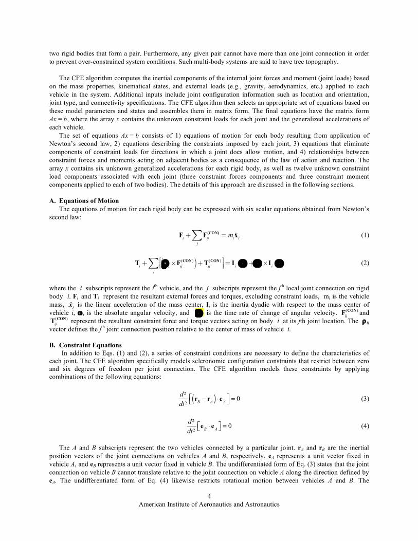
The sample multi-body system depicted in Fig. 2 shows five rigid bodies connected by four joints. The joints are indicated as solid dots labeled J1-J4, and the rigid bodies are labeled as RB1-RB5. The ρ vectors define the joint locations relative to the respective center of mass of each attached body. The CFE algorithm is implemented such that each joint connects exactly

a) External forces. b) Internal forces. c) Free body diagram. Figure 1. Decomposition of external forces and internal constraint forces to free body diagram solved by CFE method.

Figure 2: Conceptual system involving five rigid bodies connected by four joints.


4

two rigid bodies that form a pair. Furthermore, any given pair cannot have more than one joint connection in order to prevent over-constrained system conditions. Such multi-body systems are said to have tree topography.

The CFE algorithm computes the inertial components of the internal joint forces and moment (joint loads) based

on the mass properties, kinematical states, and external loads (e.g., gravity, aerodynamics, etc.) applied to each vehicle in the system. Additional inputs include joint configuration information such as location and orientation, joint type, and connectivity specifications. The CFE algorithm then selects an appropriate set of equations based on these model parameters and states and assembles them in matrix form. The final equations have the matrix form Ax = b, where the array x contains the unknown constraint loads for each joint and the generalized accelerations of each vehicle.

The set of equations Ax = b consists of 1) equations of motion for each body resulting from application of Newton’s second law, 2) equations describing the constraints imposed by each joint, 3) equations that eliminate components of constraint loads for directions in which a joint does allow motion, and 4) relationships between constraint forces and moments acting on adjacent bodies as a consequence of the law of action and reaction. The array x contains six unknown generalized accelerations for each rigid body, as well as twelve unknown constraint load components associated with each joint (three constraint forces components and three constraint moment components applied to each of two bodies). The details of this approach are discussed in the following sections.

A. Equations of Motion The equations of motion for each rigid body can be expressed with six scalar equations obtained from Newton’s

second law:

Fi+ F

ij

(CON)

j

! = mi!!x

i (1)

Ti+ !

ij!F

ij

(CON)( )+ Tij

(CON)"#$

%&'

j

( = Ii) !"

i+"

i!I

i)"

i (2)

where the i subscripts represent the ith vehicle, and the j subscripts represent the jth local joint connection on rigid body i. Fi and Ti represent the resultant external forces and torques, excluding constraint loads, mi is the vehicle mass,

!!x

i is the linear acceleration of the mass center, Ii is the inertia dyadic with respect to the mass center of

vehicle i, ω i is the absolute angular velocity, and !!

i is the time rate of change of angular velocity.

F

ij

(CON) and

T

ij

(CON) represent the resultant constraint force and torque vectors acting on body i at its jth joint location. The ρ ij vector defines the jth joint connection position relative to the center of mass of vehicle i.

B. Constraint Equations In addition to Eqs. (1) and (2), a series of constraint conditions are necessary to define the characteristics of

each joint. The CFE algorithm specifically models scleronomic configuration constraints that restrict between zero and six degrees of freedom per joint connection. The CFE algorithm models these constraints by applying combinations of the following equations:

d 2

dt2r

B! r

A( ) " eA#$

%& = 0 (3)

d 2

dt2e

B! e

A"# $% = 0 (4)

The A and B subscripts represent the two vehicles connected by a particular joint. rA and rB are the inertial position vectors of the joint connections on vehicles A and B, respectively. eA represents a unit vector fixed in vehicle A, and eB represents a unit vector fixed in vehicle B. The undifferentiated form of Eq. (3) states that the joint connection on vehicle B cannot translate relative to the joint connection on vehicle A along the direction defined by eA. The undifferentiated form of Eq. (4) likewise restricts rotational motion between vehicles A and B. The


5

constraints are differentiated twice to yield equations constraining the generalized accelerations for inclusion in the system matrix equations.

C. Joint Degrees of Freedom In contrast to more conventional Lagrange Multiplier methods,19-20 the number of multipliers employed in the

CFE algorithm can be regarded as more than absolutely necessary. This redundancy is introduced in the interest of generality in the algorithm. As a result, additional information is needed in conjunction with Eqs. (3) and (4) to solve the system. Specifically, each joint is assigned between one and six scalar equations of the form of (3) and (4), depending on the number of constrained degrees of freedom. The constraint load components must be set to zero for all remaining degrees of freedom not restricted by Eqs. (3) and (4). This can be stated mathematically as follows.

F

B

(CON)! e = 0 (5)

T

B

(CON)! e = 0 (6)

where F

B

(CON) and T

B

(CON) represent the constraint force and torque vectors acting at the joint connection on vehicle B, and e is a unit vector which is aligned with the appropriate degree of freedom. These constraining forces and moments are the additional external forces and moments provided by CFE, as illustrated in Fig. 1(c).

As an example, a revolute joint prevents all relative joint displacement from occurring between vehicles A and B, and only allows rotation about a single axis. This single degree of freedom joint is specified using three equations of form (3), and two equations of form (4). Since the revolute joint has no torque resistance about its axis of rotation, we must additionally add Eq. (6) with e set to a unit vector along the axis of rotation. For a prismatic joint, Eq. (5) would be used and e is a unit vector in the direction of permitted translation.

In summary, each joint must employ a total of six scalar equations of the form of Eqs. (3), (4), (5), and (6) appropriate to the joint type. Since the constraint loads are modeled separately for each connected vehicle, there are a total of twelve unknown scalar components for each joint. This implies that six additional equations are needed to account for the remaining unknowns. The equations in the following section provide these additional six equations.

D. Law of Action and Reaction In constructing Eqs. (1) and (2), the constraint force

acting on one body, A, is regarded as independent of the constraint force acting on the body B to which A is connected. Likewise, the constraint torque exerted on A is regarded as unrelated to the torque applied to B. However, the law of action and reaction provides six scalar relationships that must be taken into account at each joint. For cases where the joint connections remain coincident, the constraint loads acting between vehicles A and B are equal in magnitude and opposite in direction as specified by Newton’s Third Law. However, the relationship is not as simple when a translational joint is involved (Fig. 3), because it allows the A and B joint connections to separate along a straight line. In general, all translational offsets result in a moment arm that must be accounted for. To capture this fact as well as relate the constraint loads acting between the A and B vehicle pair, the following equations are used:

F

A

(CON)+ F

B

(CON)= 0 (7)

T

A

(CON)+ T

B

(CON)+ r

B! r

A( ) " F

B

(CON)= 0 (8)

Figure 3. Illustration of a 1-D prismatic joint connection between two rigid bodies. The load-balancing equations relate the A and B constraint load components acting at the respective A and B connection positions.


6

Note that Eq. (8) gives a simple, expected result when no translation is permitted (rA = rB).

E. Baumgarte Stabilization Technique Equations (1) through (8) represent a sufficient set for solving the general constraint load problem described

herein. However, the accuracy of the constraint load solution is sensitive to computational numerical error and initial joint misalignment. In particular, an accumulation of numerical error typically manifests itself as joint separation and/or misalignment over time. This in turn introduces additional errors in the solution, and the cycle continues. In order to reduce or even reverse joint separation and misalignment errors, the CFE algorithm implements an optional stabilization technique known as Baumgarte stabilization.20 Ordinarily, the constraint Eqs. (3) and (4) take the following form:

f = !!g = 0 , (9)

where g represents either of the (non-differentiated) configuration constraint equations:

rB! r

A( ) " e

A= 0

e

B! e

A= 0 (10)

The stabilization technique is implemented by augmenting Eq. (9) with terms involving the once-differentiated and non-differentiated forms of g:

f = !!g + 2! !g +!2g = 0 (11)

Thus the new constraint relation in Eq. (11) considers not only the acceleration constraints, but also the corresponding velocity and original configuration constraints. These additional terms serve as a form of proportional and derivative control which can curtail joint separation and misalignment errors. Since the stabilization effect is dependent on the specific dynamic system, the parameter η can be tuned to control the degree of constraint error.

F. Combined System Matrix and Solution The CFE algorithm applies Eqs. (1) through (11) based on the complete multi-body system model and assembles

a combined system matrix equation of the form Ax = b. As previously stated, the array x contains the unknown constraint loads for each joint and the generalized accelerations of each vehicle (which are not directly used). All constraint loads are computed in inertial frame components and then resolved to local body coordinates of the respective vehicles. The matrix equation is computed at each simulation time step and solved using a standard matrix inversion routine. The CFE algorithm currently implements Crout’s method using partial pivoting,22 an LU decomposition algorithm. Once obtained, the constraint loads are applied back to the appropriate POST2 vehicles as external loads.

III. Results and Discussion

A. Test Case #1: Constraint Force Equation Verification In order to verify the stand-alone form of the constraint force equation methodology, a simple test problem was

constructed consisting of three rigid bodies connected by two joints. The initial orientation of the three bodies is shown in Fig. 4. Relative motion between the bodies was constrained by two different joint types. Rigid Body 1 (RB1) was connected to RB2 by a revolute (pinned) joint that constrained all relative translational motion and permitted relative rotation only about the joint axis. RB1 was also connected to RB3 by a fixed joint that constrained all relative translational and rotational motion between the two bodies. Thus, in this test case, RB1 and RB3 act together essentially as a single rigid body but serve as a good test for CFE to satisfy this constraint.

Also listed in Fig. 4 are the mass properties of each body and the time-varying loads that were applied to RB1 and RB2. The dynamic motion of this multi-body configuration was simulated using ADAMS/Solver, where the two different joint type combinations were simulated using built-in joint models in ADAMS. Simulations were


7

performed using the GSTIFF integrator, a variable order (maximum 6th), variable step, multi-step integration routine. The GSTIFF integrator is the most widely used and tested integrator in ADAMS/Solver. Simulations were run for 20 s using a maximum time step of 0.005 s and an error tolerance of 1.0e-8.

Figure 4. Screen capture from ADAMS/View showing initial orientation of rigid bodies for Test Case #1.

Time histories of the body states, constraint forces and constraint torques were generated in ADAMS/Solver.

The state information from this solution (e.g., angular velocities, transformation matrices, etc.) was subsequently input into the CFE algorithm along with mass properties, joint locations and axis of rotation data in order to generate an independent time history of the constraint forces and torques. The constraint forces and torques that were computed with the CFE method were compared to the ADAMS/Solver results as the truth model, to evaluate the performance of the CFE methodology.

The level of agreement between the ADAMS/Solver and the CFE algorithm is shown in Fig. 5, where time histories of the constraint forces and constraint torques are plotted for the entire duration of 20 s. Since the rotation axis of the revolute joint was aligned with the body Z-axis, the Z-component of the constraint torque was zero; permitting relative rotation about the body Z-axis between Bodies 1 and 3. To better illustrate the level of agreement between the two solutions, the same data is shown for the last second of the simulation in Fig. 6. Finally, Fig. 7 shows the percent error of the CFE results with respect to the ADAMS/Solver solution. For much of the simulation, the percent error is below one percent. The isolated spikes in error occur when that particular force or torque value passes through zero.

Figures 8-10 illustrate a similar comparison of the constraint loads for the fixed joint connecting Bodies 1 and 3. The results indicate the same level of agreement between the CFE results and ADAMS/Solver solution as achieved for the revolute joint.


8

Figure 5. Constraint force and torque comparison: Standalone CFE vs ADAMS for Joint 1 (revolute).

Figure 6. Constraint force & torque comparison: Standalone CFE vs ADAMS for Joint 1 (revolute)

(enlargement of last 1 s).


9

Figure 7. Constraint force and torque comparison: Percent Error between Standalone CFE and

ADAMS for Joint 1 (revolute).

Figure 8. Constraint force and moment comparison: Standalone CFE vs ADAMS for Joint 2 (fixed).


10

Figure 9. Constraint force and torque comparison: Standalone CFE vs ADAMS for Joint 2 (fixed)

(enlargement of last 1 s).

Figure 10. Constraint force and torque comparison: Percent Error between Standalone CFE and ADAMS

for Joint 2 (fixed).


11

B. Test Case #2: TSTO Bimese Vehicle Stage Separation A two-stage-to-orbit (TSTO) Bimese Vehicle stage separation

problem was selected as the test case for CFE implementation in POST2. A schematic diagram of the TSTO Bimese vehicle concept, in which both the orbiter and the booster have the same external shape, is shown in Fig. 11. The relative arrangement of the two vehicles is shown in Fig. 12. The booster (first stage) is attached to the orbiter (upper stage) at two points. Prior to the release, the forward joint is assumed to be a fixed support and the aft joint is assumed to permit rotation in pitch. The relative location of these vehicles during separation is depicted in Fig. 13. Additional details of the vehicle mass properties, aerodynamic and propulsion characteristics, and flight parameters at staging can be found in Ref. 15.

A sample case of stage separation for this vehicle was created with the purpose of demonstrating the joint modeling capability between two 6-DOF rigid bodies and verifying against results generated with ConSep/ADAMS. This solution generated by ConSep/ADAMS is different from the complete simulation of stage separation as discussed in Ref. 15.

The separation sequence that was employed is shown in Fig. 14. For simplicity, both vehicles are initially rigidly fastened by a single fixed joint located at the rear attachment point with aerodynamic loads applied to both vehicles and a thrust force applied to the booster. At 0.3 s, a separation load is applied to the booster to test the fixed joint constraint equations. At 0.5 s, the fixed joint is replaced with a pinned joint and the booster begins to rotate about the y axis of the orbiter at the joint location. At 1.5 s, the joint is released and the separation load is removed. The simulation ends at 3 s.

Figure 15 shows the constraint forces and torques computed by both the POST and ConSep simulations. There is excellent agreement between the results computed by each simulation. The y-force and x and z-torques are essentially zero, which is expected since all motion occurs in the pitch plane (lateral-directional aerodynamic forces were not

Figure 11. Schematic diagram of the Bimese Vehicle modeled in Test #2.

Figure 13. Relative locations of the Bimese vehicles during separation.

Figure 12. Schematic illustration of the attachment of the booster and orbiter.

Figure 14. Separation timeline for Test Case #2.


12

included in the simulation). Also, note that the y-constraint torque goes to zero at 0.5 s as expected since that is when the fixed joint was changed to a pinned joint.

Figure 15. Comparison of constraint force and moments: Consep vs. POST2 with CFE.

One metric used to evaluate the performance of the CFE methodology is the relative joint displacement between

the two separating vehicles. This parameter is the total distance from the booster joint location to the orbiter joint location. For the first 1.5 s, when the joint constraint is active, the relative joint displacement should be zero; that is, the internal forces and moments determined using the CFE technique should be keeping the two vehicles joined at the location of the joint. Since the CFE method that is implemented in POST2 integrates each body separately with constraint forces applied as external forces, the accumulation of numerical error will cause the vehicles to slowly separate at the joint location such that the joint displacement will be non-zero. The extent to which the joint constraint is violated is directly measured by computing the relative joint displacement.

Figure 16 shows the relative joint displacement plotted as a function of time for a series of simulations conducted in POST2. The baseline curve is for the case with, η, the Baumgarte Error Stabilization factor, set to zero. The figure shows that even without error stabilization, the constraint is reasonably well satisfied since the relative joint displacement distance remains below 0.015 ft (0.024% of the total vehicle length) for the first 1.5 s, the entire duration that the vehicles are joined. However, by including the error stabilization term, the joint displacement distance can be reduced by a factor of 2.4 when η = 1. The improvement tends to progressively increase as η is increased, and the displacement error is reduced by two orders of magnitude when η = 10. For this case, higher values may be too large as indicated by the slight increase in joint separation after ~1.35 s for the η = 50 case. In addition, values of η that are too large actually result in an increase in joint separation for the first ~0.38 s as compared to the baseline η = 0 case.


13

Figure 16. Effect of error stabilization coefficient η on relative joint displacement for POST2 CFE cases.

Figure 17 compares the angle-of-attack time histories for the orbiter for the baseline η = 0 and η = 10 cases with

the ConSep results. There is good agreement between all three cases, but clearly the improvement in joint constraint compliance from the inclusion of error stabilization also improves the conformity between the CFE and ConSep attitude time history results. Similar agreement was obtained for booster angle of attack and other flight path variables not shown here.

Figure 17. Angle of attack time history comparison for bimese orbiter: ConSep vs POST2 CFE with two

different error stabilization coefficients.


14

The good agreement between the POST2/CFE results and ConSep/ADAMS for these two test cases

demonstrates that the constraint force equation methodology is suitable for simulating stage separation problems in the POST2 environment. When this capability is added to POST2, it will be possible to perform seamless end-to-end mission simulation for multi-stage launch vehicles that have complex joint interfaces.

IV. Concluding Remarks The constraint force equation (CFE) methodology was developed in a stand-alone mode for modeling constraint

forces and moments acting on multiple bodies connected with simple joints, permitting arbitrary degree of freedom and suitable for simulation of multi-body separation in launch vehicle staging environment. The CFE methodology was implemented in the industry standard trajectory simulation tool POST2 to add the capability to perform end-to-end simulation of launch vehicle trajectories. Two test cases were discussed in this paper. The first case examined the motion of three rigid bodies connected with one fixed and one revolute joint in order to demonstrate the CFE methodology. The second case simulated the stage separation of a bimese TSTO vehicle to validate the CFE implementation in POST2. For both cases, the CFE results were in good agreement with those generated using ConSep/ADAMS, verifying the CFE methodology and its implementation in POST2. However, additional testing and verification of the POST2/CFE methodology are needed before this code is ready for generic end-to-end simulation of launch vehicle trajectories.

V. Acknowledgements The authors would like to gratefully acknowledge Anne Rhodes for her invaluable assistance in preparing this

paper for publication. The author would also like to thank Carlos Roithmayr for thoroughly reviewing the manuscript and making numerous suggestions and enhancements that have significantly improved the clarity of the final paper. Finally, the authors would like to thank Chris Karlgaard for his helpful technical consultation and advice.

References 1Dillenius, M.F.E., Perkins, S.C., and Nixon, D., Pylon Carriage and Separation of Stores, AIAA Progress in Astronautics

and Aeronautics: Tactical Missile Aerodynamics-General Topics, M.J.Hemsch, ed., Vol. 141, 1992. 2Taylor, R.T., and Alford, W. J, Jr., A wind tunnel investigation of the carry loads and mutual interference effects of 1/40-

scale models of the X-15 and B-52 airplanes in combination, NASA TM X-184, December 1959. 3Decker, J.P., and Wilhite, A. W., Technology and Methodology of Separating Two Similar Size Aerospace Vehicles Within

the Atmosphere. AIAA Paper 1975-29, Jan. 1975. 4Decker, J. P., Experimental Aerodynamics and Analysis of the Stage Separation of Reusable Launch Vehicles. NASA-SP-

148, January 1967. 5Decker, J. P., and Gera, J., An Exploratory Study of Parallel-Stage Separation of Reusable Launch Vehicles. NASA TN D-

4765, October 1968. 6Decker, J. P., Aerodynamic Interference Effects Caused by Parallel-Staged Simple Aerodynamic Configuration at Mach

Numbers of 3 and 6. NASA TN D-5379, Aug. 1969. 7Wilhite, A. W., Analysis of Separation of the Space Shuttle Orbiter from a Large Transport Airplane. NASA TM X-3492,

June 1977. 8Naftel, J. C., and Wilhite, A.W., Analysis of Separation of a Two-Stage Winged Launch Vehicle. AIAA Paper 86-0195, Jan.

1986. 9Naftel, J. C., and Powell, R.W., Aerodynamic Separation and Glideback of a Mach 3 Staged Orbiter. AIAA Paper 90-0223,

Jan. 1990. 10Naftel, J. C., and Powell, R. W., Analysis of the Staging Maneuver and Booster Glideback Guidance for a Two-Staged,

Winged, Fully Reusable Launch Vehicle. NASA TP-3335, 1993. 11Murphy, K.J., Buning, P.G., Pamadi, B.N., Scallion, W.I., and Jones, K.M.; Status of Stage Separation Tool Development

for Next Generation Launch Vehicle Technologies. AIAA Paper 2004-2595. 12Using ADAMS/Solver, Mechanical Dynamics, Inc., 1999. 13Tartabini, P. V., Bose, D. M., McMinn, J. D., Martin, J. G., and Strovers, B. K., Hyper-X Stage Separation Trajectory

Validation Studies, AIAA Paper 2003-5819, August 2003. 14Pamadi, B.N., Neirynck, T. A., Covell, P.F., Hotchko, N.J., and Bose, D.M., Simulation and Analyses of Staging

Maneuvers of Next Generation Reusable Launch Vehicles, AIAA Paper 2004-5185. 15Pamadi, B.N., Neirynck, T. A., Hotchko, N.J., Scallion W.I., Murphy, K.J., and Covell, P.F., Simulation and Analyses of

Stage Separation of Two-Stage Reusable Launch Vehicles, Journal of Spacecraft and Rockets, Vol. 44, No. 1, January-February 2007, pp 66-80.


15

16Pamadi, B.N., Hotchko, N.J., Jamshid Samareh, Covell, P.F., and Tartabini, P.V., Simulation and Analyses of Multi-Body Separation in Launch Vehicle Staging Environment, AIAA Paper 2006-8033.

17 Brauer, G. L., Cornick, D. E., and Stevenson, R., “Capabilities and Applications of the Program to Optimize Simulated Trajectories (POST),” NASA CR-2770, Feb. 1977.

18 Powell, R. W., et. al., “Program to Optimize Simulated Trajectories (POST2) Utilization Manual, Version 1.1.7,” July 2002.

19 Arabyan, A., Wu, F., An Improved Formulation for Constrained Mechanical Systems, Multibody System Dynamics 2, pp. 49–69, 1998.

20 Blajer, W., On the Determination of Joint Reactions in Multibody Mechanisms, Journal of Mechanical Design, Vol. 126, pp. 341–350, March 2004.

21 Baumgarte, J., Stabilization of Constraints and Integrals of Motion in Dynamical Systems, Computer Methods in Applied Mechanics and Engineering 1, pp. 1–16, 1972

22 Press, W. H., et. al.,, Numerical Recipes in C, The Art of Scientific Computing, Second Edition, Cambridge University Press, pp. 43–48, 1992.

Constraint Force Equation Methodology for Modeling Multi-Body Stage Separation Dynamics

Paul V. Tartabini Mathew Toniolo Bandu Pamadi

NASA Langley Research Center Hampton, Virginia

Proposed Abstract for the

AIAA Aerospace Sciences Meeting and Exhibit January 7-10, 2008

Reno, Nevada

Problem

In NASA’s Next Generation Launch Technology (NGLT) Program, stage separation was identified as a critical technology needed for successful development and operation of multi-stage reusable launch vehicles. As a step towards developing this critically needed technology, NASA has initiated a comprehensive stage separation tool development activity that includes wind tunnel testing, development and validation of CFD and engineering level tools. A key part of this activity is the development of a generalized stage separation analysis and simulation capability to perform the design and evaluation of separation strategies for nominal and abort scenarios.

In response to this need, a conceptual level tool called ConSep was created using the Automatic Dynamic Analysis of Mechanics Systems (ADAMS) Simulation software.1 ADAMS is a high fidelity solver capable of simulating complex mechanical systems. To simulation the stage separation problem, various user-defined modules were developed to provide flexibility in modeling vehicle aerodynamics, propulsion, connection joints, separation forces, control laws, and actuators. The entire simulation, which includes the user-defined modules wrapped around the ADAMS solver, is known as ConSep.2 This generic tool was derived from a specialized simulation called SepSim that was developed in support of the successful X-43A flight project.3

The generality provided from the specialized ADAMS solver enables the modeling of complex separation problems with multiple joints and a range of possible joint types. That generality, however, increases the overall complexity of the problem since the flight mechanics modeling must be added separately (e.g., user-defined modules for aerodynamics, etc.). Moreover, to perform an end-to-end simulation, at least two codes are required: a trajectory simulation program for the flight segments before and after staging, and the ADAMS-based multi-body dynamics simulator for the stage separation event. Such a scheme is more complex than using a single code, and often much slower, thus making it more difficult to perform trajectory optimization and Monte Carlo analyses. In addition, having more than one code provides additional challenges in simulation verification.

This paper discusses an alternate approach for modeling stage separation problems using a widely available trajectory design and optimization tool. Instead of employing a separate code to simulate the stage separation flight segment, the capability to model internal constraint forces due to simple joints connecting multiple rigid bodies was added to the trajectory software. This technique enables an entire end-to-end simulation to be performed with a single code, thus simplifying the overall implementation as well as providing a range of modeling and optimization capabilities that are standard features in most trajectory software packages.

Approach

This paper describes a generic stage separation simulation developed using the Program to Optimize Simulated Trajectories (POST II).4-5 POST II is a generalized trajectory optimization program that can be used to model three and six-degree-of-freedom trajectories for multiple powered or unpowered vehicles. The original POST program was first developed in the early 1970’s and has been continuously developed and improved since that time. POST II draws on this heritage while incorporating numerous improvements and enhancements to the original POST, not the least of which is the ability to simultaneously simulate more than one vehicle. This new capability, as well as the fact that the program can be easily modified by an experienced user to include vehicle control systems and non-standard trajectory models, made POST II an appropriate choice for the construction of end-to-end trajectory simulation tool. Furthermore, the POST II architecture provided optimization capabilities to determine how control system inputs and other design variables can be adjusted to optimize the trajectory profile during separation.

To model the internal constraint forces within POST II, analytical expressions were derived for the forces and torques necessary to maintain the kinematical constraints imposed by a single fixed, pinned, or ball joint connecting two rigid bodies with six degrees of freedom (6-DOF). The joint location on each body was arbitrary, but was assumed to remain fixed relative to each vehicle. These analytical expressions were generated by inverting an 18 x 18 matrix and were included in a FORTRAN subroutine that calculated the constraint loads as a function of the kinematic state, joint location, axis of rotation, external loads and mass properties of each body. Figure 1 shows the general formulation of the equations of motion and kinematical constraint equations for the fixed and pinned joint cases.

Summary of Important Conclusions

A sample case was created to demonstrate the joint modeling capability between two 6-DOF rigid bodies and was verified against results generated with ConSep. The sample problem modeled the stage separation of bimese reusable launch vehicles, a two-stage-to-orbit concept in which both the booster and orbiter have the same outer-mold lines. Figure 2 is a schematic illustration showing the location of the two attachment points on the vehicles prior to separation. The forward joint is assumed to be a fixed support and the aft joint is assumed to permit rotation in pitch. The separation sequence that was employed is shown in Fig. 3. For simplicity, both vehicles are initially rigidly

fastened by a single fixed joint and no loads are applied. At 0.3 sec a separation load is applied to vehicle 1 to test the fixed joint constraint equations. At 0.5 sec the fixed joint is replaced with a pinned joint with the rotation axis directed along the y-axis of the orbiter and the vehicle begins to rotate about the joint location. At 1.5 sec the joint is released and the separation load is removed. The simulation ends at 3 sec.

Figure 4 shows the constraint forces and torques computed by both the POST and ConSep simulations. There is excellent agreement between the results computed by each simulation. The y-force and x and z-torques are essentially zero which is expected since all motion occurs in the pitch plane (lateral-directional aerodynamic forces were not included in the simulation). Also, note that the y-constraint torque goes to zero at 0.5 sec as expected since that is when the fixed joint was changed to a pinned joint.

The angle-of-attack time histories for each vehicle are shown in Figure 5. Again, the results from each simulation match very well. In addition, the relative joint displacement between the two vehicles is plotted in Fig. 6. This parameter defines the distance between the joint contact points on each vehicle and should be zero while the vehicles are still attached. The figure shows that the constraint is reasonably well satisfied since the distance remains below 0.02 inches for the entire duration that the vehicles are joined.

References

1 Anon.: Using ADAMS/Solver. Users Guide, Vol. 9.0.1, Mechanical Dynamics, Inc. 2 Pamadi, B. N., Neirynck, T. A., Hotchko, N. J., Tartabini, P. V., Scallion, W. I., Murphy, K. J., and Covell, P. F.,

“Simulation and Analyses of Stage Separation Two-Stage Reusable Launch Vehicles,” AIAA Paper 2005-3247, May, 2005.

3 Tartabini, P. V., Bose, D. M., McMinn, J. D., Martin, J. G., and Strovers, B. K., “Hyper-X Stage Separation Trajectory Validation Studies,” American Institute of Aeronautics and Astronautics, AIAA Paper 2003-5819, August 2003.

4 Brauer, G. L., Cornick, D. E., and Stevenson, R., “Capabilities and Applications of the Program to Optimize Simulated Trajectories (POST),” NASA CR-2770, Feb. 1977.

5 Powell, R. W., et. al., “Program to Optimize Simulated Trajectories (POST II) Utilization Manual, Version 1.1.7,” July 2002.

Figure 1. Equations of motion and kinematical constraint equations for fixed and pinned joint cases.

Figure 2. Schematic illustration of the attachment of the booster and orbiter.

Figure 3. Separation event sequence for sample bimese stage separation problem.

Figure 4. Comparison of constraint forces computed by POST and ConSep. Vehicle 1 is the orbiter and Vehicle 2 is the booster.

Figure 5. Angle-of-attack time history comparison. Vehicle 1 is the orbiter and Vehicle 2 is the booster.

Figure 6. Relative joint location distance between booster and orbiter.

Documents

Constraint Force Equation Methodology for Modeling Multi-Body … · Constraint Force Equation Methodology for Modeling Multi-Body Stage Separation Dynamics Matthew D. Toniolo*