Constraint Routing and Regenerator Site Concentration in ...lightwave.ee.columbia.edu/Publications/Bathula2013.pdf · Constraint Routing and Regenerator Site Concentration in ROADM

Constraint Routing and Regenerator SiteConcentration in ROADM Networks

Balagangadhar G. Bathula, Rakesh K. Sinha, Angela L. Chiu, Mark D. Feuer, Guangzhi Li,Sheryl L. Woodward, Weiyi Zhang, Robert Doverspike, Peter Magill, and Keren Bergman

Abstract—Advances in the development of colorless andnondirectional reconfigurable optical add–drop multi-plexers (ROADMs) enable flexible predeployment ofoptoelectronic regenerators (reshaping, retiming, andreamplifying known as 3R) in future optical networks.Compared to the current practice of installing a regenera-tor only when a circuit needs them, predeployment ofregenerators in specific sites will allow service providersto achieve rapid provisioning such as bandwidth-on-demand service and fast restoration. Concentrating thepredeployment of regenerators in a subset of ROADM siteswill achieve high utilization and reduces the networkoperational costs. We prove the resulting optimizationproblem is NP-hard and provide the proof. We present anefficient heuristic for this problem that takes into accountboth the cost of individual circuits (regenerator cost andtransmission line system cost) and the number of regener-ator sites. We validate our heuristic approach with integerlinear programming (ILP) formulations for a small net-work. Using specific network examples, we show that ourheuristic has near-optimal performance under moststudied scenarios and cost models. We further enhancethe heuristic to incorporate the probability of demand foreach circuit. This enables a reduction in the number ofregenerator sites by allowing circuits to use costlier pathsif they have lower probability of being needed. We alsoevaluate the heuristic to determine the extra regeneratorsites required to support diverse routing. In this paper,we provide detailed analysis, pseudocodes, and proofsfor the models presented in our previous work [Nat. FiberOptic Engineers Conf., 2012, NW3F.6; 9th Int. Conf. onDesign of Reliable Communication Networks (DRCN),2013, 139] and compare the heuristic results with ILP fora small-scale network topology.

IndexTerms—All-optical networks; Network optimization;Reconfigurable optical-add–drop multiplexer (ROADM);Regenerator placement.

I. INTRODUCTION

T raffic on backbone networks has increased by fourorders of magnitude over the past 12 years and esti-

mates on the growth rate going forward vary from 30% to40% per year [1]. Though there has been rapid growth in

traffic, the revenues of the telecommunication carrierare not keeping pace with this explosive growth. In orderto bridge the gap and to sustain this traffic growth, thecost-effectiveness of optical networks must continue to im-prove. To date, advances in optical networks have mainlybeen in three areas: 1) improvements in fiber capacity, 2)improvements in optical reach (the distance over whicha wavelength signal can be transmitted with adequatefidelity), and 3) the development and widespread adop-tion of reconfigurable optical add–drop multiplexers(ROADMs). If a circuit’s path is longer than the system’soptical reach (typically 1500–2800 km for modern long-haul systems), then one or more optoelectronic regenera-tors must be used to restore the signal, and eachregenerator adds a cost comparable to a pair of endpointtransceivers. ROADMs enable any wavelength to bypassa node, terminate at the node, or be regenerated to main-tain signal quality. Optical bypass allows operators todeploy far fewer transponders and regenerators, yieldingsignificant cost savings [2–4]. At junction nodes wheremore than two fiber pairs meet, ROADMs also allow wave-length routing from any link to any other link, forming anoptical mesh network.

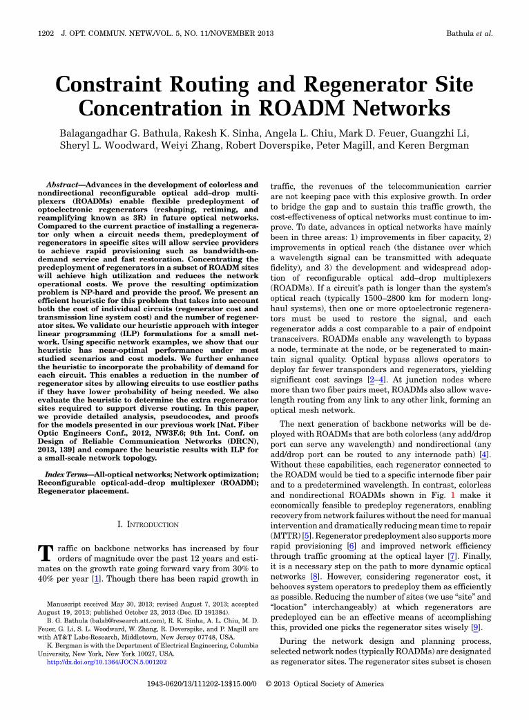
The next generation of backbone networks will be de-ployed with ROADMs that are both colorless (any add/dropport can serve any wavelength) and nondirectional (anyadd/drop port can be routed to any internode path) [4].Without these capabilities, each regenerator connected tothe ROADM would be tied to a specific internode fiber pairand to a predetermined wavelength. In contrast, colorlessand nondirectional ROADMs shown in Fig. 1 make iteconomically feasible to predeploy regenerators, enablingrecovery fromnetwork failureswithout the need formanualinterventionanddramatically reducingmean time to repair(MTTR) [5]. Regenerator predeploymentalso supportsmorerapid provisioning [6] and improved network efficiencythrough traffic grooming at the optical layer [7]. Finally,it is a necessary step on the path to more dynamic opticalnetworks [8]. However, considering regenerator cost, itbehooves system operators to predeploy them as efficientlyas possible. Reducing the number of sites (we use “site” and“location” interchangeably) at which regenerators arepredeployed can be an effective means of accomplishingthis, provided one picks the regenerator sites wisely [9].

During the network design and planning process,selected network nodes (typically ROADMs) are designatedas regenerator sites. The regenerator sites subset is chosenhttp://dx.doi.org/10.1364/JOCN.5.001202

Manuscript received May 30, 2013; revised August 7, 2013; acceptedAugust 19, 2013; published October 23, 2013 (Doc. ID 191384).

B. G. Bathula ([email protected]), R. K. Sinha, A. L. Chiu, M. D.Feuer, G. Li, S. L. Woodward, W. Zhang, R. Doverspike, and P. Magill arewith AT&T Labs-Research, Middletown, New Jersey 07748, USA.

K. Bergman is with the Department of Electrical Engineering, ColumbiaUniversity, New York, New York 10027, USA.

1202 J. OPT. COMMUN. NETW./VOL. 5, NO. 11/NOVEMBER 2013 Bathula et al.

1943-0620/13/111202-13$15.00/0 © 2013 Optical Society of America

http://dx.doi.org/10.1364/JOCN.5.001202

to ensure that regenerators can be placed among the setto satisfy the optical reach constraint for every possibledemand. In some cases, additional requirements may alsobe placed on the routes allowed for a demand. The problemof picking a minimum set of regenerator sites RS is definedas the regenerator location or placement problem (RLP)[10,11]. The problem has been studied in two flavors:1) the unconstrained-routing regenerator location problem(URLP) and 2) the explicit-routing regenerator locationproblem (ERLP). URLP does not limit circuit routing inany way. While the solution may be optimal in a numberof regenerator locations, individual circuits may incurhigh cost as a result of using longer routes or using moreregenerators. ERLP constrains each route to a specified(typically min-distance) path, but individual circuits mayuse more regenerators than necessary. Reference [12]proves that URLP is NP-hard. The authors of [12] also pro-pose and compare three heuristics for URLP. Reference [13]uses a biased random-key genetic algorithm to solve theURLP with improved results. Reference [14] proves thehardness of several different variants of the regeneratorplacement problem and gives approximation algorithmswith worst-case performance guarantees.

Most previous RLPs have focused on minimizing thenumber of regenerator sites while still being able to routea circuit between any node pair [15,16]. While minimizingthe number of sites is an important consideration, it shouldbe balanced with the sum of the cost of individual circuits.So there are two additional major considerations to theoverall network cost: 1) the cost of an individual circuit de-pends on the number of regenerators used as well as itstransmission distance and 2) traffic demands in productionnetworks tend to be highly nonuniform, meaning that theprobability of a demand varies greatly among node pairs.

We take a holistic view of minimizing overall networkcost by considering all three factors. We have proposed anew routing-constrained regenerator location problem[17] that constrains the connections to use least-cost paths(including the cost of regeneration). The cost model can beextended to include the transmission distance (whichaffects the cost of fiber, buildings, and amplifiers), as wellas the regenerator count. For some customers with strictlatency requirements, shorter transmission paths are

needed, above and beyond the cost of the optical path. Webuild upon the routing-constrained regenerator locationproblem in [17] to take into account these additional prac-tical considerations. The heuristics also incorporate [18] aprojected traffic matrix to explore the trade-off betweenthe cost of each circuit and the number of jRSj. For exam-ple, if a node pair is unlikely to have significant traffic, itspath could be slightly more costly than the minimum costpath—if that enables jRSj to be further reduced. In ourheuristic, the allowable path cost deviation for each nodepair is roughly inversely proportional to the probabilityof a connection between that node pair. The overall goalremains to minimize the total network cost, defined as thesum of a per-site cost and the total cost of active circuits.This paper goes beyond that presented in [18] by providingmore detailed proofs, pseudocodes, integer linear program-ming (ILP) formulation for the problem, and comparison ofthe heuristic solution with ILP on a small-scale networktopology.

The rest of the paper is organized as follows. InSection II, we start by defining a simple version of the prob-lem where the cost of a circuit is given solely by the numberof regenerators being used. We illustrate the problem witha small example network and provide a proof of NP-hardness. In Section III, we explain the proposed heuristicapproach for reducing the regenerator sites and networkcosts and describe several variations. A lower bound onthe optimal solution is provided. In Section IV, we proposea trade-off for reducing the number of regenerator sites byallowing a small increase in the cost of low-probabilitycircuits. We determine the extra regenerator sites neededfor link-disjoint paths in Section V. Section VI containsthe experimental evaluation results of our algorithms onlarge-scale network topologies. Finally, in Section VII, wesummarize the work and outline possible extensions.

II. PROBLEM DEFINITION

We start by defining a version of the problem where thecost of a circuit is given only by the number of regeneratorsbeing used (in most cases, this is the dominant variablecomponent of the circuit cost). The goal is to minimizethe number of regenerator sites subject to the constraintthat each circuit uses a minimum possible number ofregenerators. This allows us to present the main ideas ofthe heuristic in a simple setting. Then as we add moreparameters to the problem, we outline the necessarychanges to the heuristic.

Let minregen�u; v� be the minimum number of regener-ators needed on any route between nodes u and v assumingthat regenerators are available at all nodes. A route Puv

between nodes u and v is called a constrained route if ituses minregen�u; v� regenerators. The constrained-routingregenerator location problem (CRLP) can be formallydefined as follows: given network topology with link distan-ces, and maximal optical reach distance, find a minimumset of RS such that between each node pair, at least oneconstrained route is reachable using a subset of regenera-tors in RS.

Fig. 1. Colorless and nondirectional ROADM.

Bathula et al. VOL. 5, NO. 11/NOVEMBER 2013/J. OPT. COMMUN. NETW. 1203

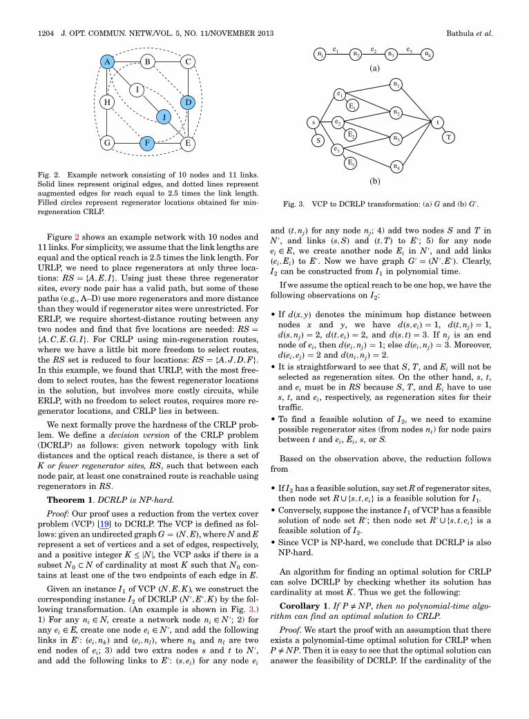
Figure 2 shows an example network with 10 nodes and11 links. For simplicity, we assume that the link lengths areequal and the optical reach is 2.5 times the link length. ForURLP, we need to place regenerators at only three loca-tions: RS � fA;E; Ig. Using just these three regeneratorsites, every node pair has a valid path, but some of thesepaths (e.g., A–D) use more regenerators and more distancethan they would if regenerator sites were unrestricted. ForERLP, we require shortest-distance routing between anytwo nodes and find that five locations are needed: RS �fA;C;E;G; Ig. For CRLP using min-regeneration routes,where we have a little bit more freedom to select routes,the RS set is reduced to four locations: RS � fA; J;D; Fg.In this example, we found that URLP, with the most free-dom to select routes, has the fewest regenerator locationsin the solution, but involves more costly circuits, whileERLP, with no freedom to select routes, requires more re-generator locations, and CRLP lies in between.

We next formally prove the hardness of the CRLP prob-lem. We define a decision version of the CRLP problem(DCRLP) as follows: given network topology with linkdistances and the optical reach distance, is there a set ofK or fewer regenerator sites, RS, such that between eachnode pair, at least one constrained route is reachable usingregenerators in RS.

Theorem 1. DCRLP is NP-hard.

Proof: Our proof uses a reduction from the vertex coverproblem (VCP) [19] to DCRLP. The VCP is defined as fol-lows: given an undirected graphG � �N;E�, whereN andErepresent a set of vertices and a set of edges, respectively,and a positive integer K ≤ jNj, the VCP asks if there is asubset N0 ⊂ N of cardinality at most K such that N0 con-tains at least one of the two endpoints of each edge in E.

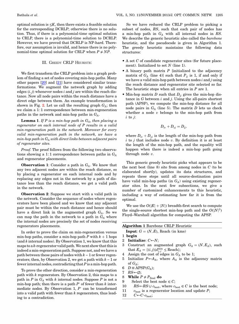
Given an instance I1 of VCP �N;E;K�, we construct thecorresponding instance I2 of DCRLP �N′; E′; K� by the fol-lowing transformation. (An example is shown in Fig. 3.)1) For any ni ∈ N, create a network node ni ∈ N′; 2) forany ei ∈ E, create one node ei ∈ N′, and add the followinglinks in E′: �ei; nk� and �ei; nl�, where nk and nl are twoend nodes of ei; 3) add two extra nodes s and t to N′,and add the following links to E′: �s; ei� for any node ei

and �t; nj� for any node nj; 4) add two nodes S and T inN′, and links �s; S� and �t; T� to E′; 5) for any nodeei ∈ E, we create another node Ei in N′, and add links�ei; Ei� to E′. Now we have graph G′ � �N′; E′�. Clearly,I2 can be constructed from I1 in polynomial time.

If we assume the optical reach to be one hop, we have thefollowing observations on I2:

• If d�x; y� denotes the minimum hop distance betweennodes x and y, we have d�s; ei� � 1, d�t; nj� � 1,d�s; nj� � 2, d�t; ei� � 2, and d�s; t� � 3. If nj is an endnode of ei, then d�ei; nj� � 1; else d�ei; nj� � 3. Moreover,d�ei; ej� � 2 and d�ni; nj� � 2.

• It is straightforward to see that S, T, and Ei will not beselected as regeneration sites. On the other hand, s, t,and ei must be in RS because S, T, and Ei have to uses, t, and ei, respectively, as regeneration sites for theirtraffic.

• To find a feasible solution of I2, we need to examinepossible regenerator sites (from nodes ni) for node pairsbetween t and ei, Ei, s, or S.

Based on the observation above, the reduction followsfrom

• If I2 has a feasible solution, say setR of regenerator sites,then node set R∪ fs; t; eig is a feasible solution for I1.

• Conversely, suppose the instance I1 of VCP has a feasiblesolution of node set R′; then node set R′∪ fs; t; eig is afeasible solution of I2.

• Since VCP is NP-hard, we conclude that DCRLP is alsoNP-hard.

An algorithm for finding an optimal solution for CRLPcan solve DCRLP by checking whether its solution hascardinality at most K . Thus we get the following:

Corollary 1. If P ≠ NP, then no polynomial-time algo-rithm can find an optimal solution to CRLP.

Proof. We start the proof with an assumption that thereexists a polynomial-time optimal solution for CRLP whenP ≠ NP. Then it is easy to see that the optimal solution cananswer the feasibility of DCRLP. If the cardinality of the

A B

H

G E

J

D

I

C

F

Fig. 2. Example network consisting of 10 nodes and 11 links.Solid lines represent original edges, and dotted lines representaugmented edges for reach equal to 2.5 times the link length.Filled circles represent regenerator locations obtained for min-regeneration CRLP.

S

31n n2 n4

n2

n3

n4

1n

1e

e2

E2

E3

1E

e3

1e e2 e3

(a)

(b)

t

T

s

n

Fig. 3. VCP to DCRLP transformation: (a) G and (b) G′.


optimal solution is ≤K, then there exists a feasible solutionfor the corresponding DCRLP; otherwise there is no solu-tion. Thus, if there is a polynomial-time optimal solutionto CRLP, there is a polynomial-time solution to DCRLP.However, we have proved that DCRLP is NP-hard. There-fore, our assumption is invalid, and hence there is no poly-nomial-time optimal solution for CRLP when P ≠ NP.

III. GREEDY CRLP HEURISTIC

We first transform the CRLP problem into a graph prob-lem of finding a set of nodes covering min-hop paths. Manyother papers [20] and [21] have considered similar trans-formations. We augment the network graph by addingedges �i; j� whenever nodes i and j are within the reach dis-tance. Now all node pairs within the reach distance have adirect edge between them. An example transformation isshown in Fig. 2. Let us call the resulting graph GA; thenwe claim a 1∶1 correspondence between min-regenerationpaths in the network and min-hop paths in GA.

Lemma 1. If P is a min-hop path in GA, then placing aregenerator on each internal node of P results in a validmin-regeneration path in the network. Moreover for everyvalid min-regeneration path in the network, we have amin-hop path inGA with direct links between adjacent pairsof regenerator sites.

Proof. The proof follows from the following two observa-tions showing a 1∶1 correspondence between paths in GA

and regenerator placements.

Observation 1: Consider a path in GA. We know thatany two adjacent nodes are within the reach distance, soby placing a regenerator on each internal node and byreplacing any edges not in the network by a path of dis-tance less than the reach distance, we get a valid pathin the network.

Observation 2: Suppose we start with a valid path inthe network. Consider the sequence of nodes where regen-erators have been placed and we know that any adjacentpair must be within the reach distance and hence shouldhave a direct link in the augmented graph GA. So wecan map the path in the network to a path in GA wherethe internal nodes are precisely the set of nodes receivingregenerators placements.

In order to prove the claim on min-regeneration versusmin-hop paths, consider a min-hop path P with k� 1 hops(and k internal nodes). By Observation 1, we know that thismaps to ak-regeneratorvalidpath.Wenext showthat this isindeedamin-regenerationpath. Supposenot, andwehaveapath between these pairs of nodes with k − 1 or fewer regen-erators; then, by Observation 2, we get a path with k − 1 orfewer internal nodes, contradicting thatP is amin-hoppath.

To prove the other direction, consider a min-regenerationpath with k regenerators. By Observation 2, this maps to apath in P in GA with k internal nodes. Suppose P is not amin-hop path; then there is a path P′ of fewer than k inter-mediate nodes. By Observation 1, P′ can be transformedinto a valid path with fewer than k regenerators, thus lead-ing to a contradiction.

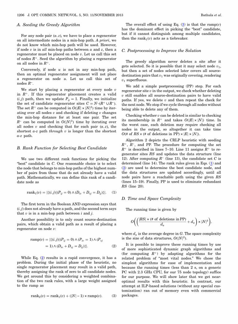
So we have reduced the CRLP problem to picking asubset of nodes, RS, such that each pair of nodes hasa min-hop path in GA with all internal nodes in RS.We describe the generic heuristic also called the bareboneheuristic, and the pseudocode is given in Algorithm 1.The greedy heuristic maintains the following datastructures:

• A set C of candidate regenerator sites (for future place-ment). Initialized to set N (line 1).

• A binary path matrix P [initialized to the adjacencymatrix of GA (line 4)] such that Pij is 1, if and only ifwe have a valid min-hop path between nodes i and j usingthe reach distance and regenerator site selected so far.The heuristic stops when all entries in P are 1.

• Min-hop matrix D such that Dij gives the min-hop dis-tance in G between i and j. Using the all-pairs shortestpath (APSP), we compute the min-hop distance for allnode pairs in GA (line 5). The matrix D lets us checkwhether a node v belongs to the min-hop path fromi to j:

Div �Dvj � Dij;

where Div �Dvj is the length of the min-hop path fromi to j that includes node v. By definition it is at leastthe length of the min-hop path, and the equality willhappen when there is indeed a min-hop path goingthrough node v.

This generic greedy heuristic picks what appears to bethe next best (line 8) site from among nodes in C (to beelaborated shortly), updates its data structures, andrepeats these steps until all source-destination pairshave valid min-hop paths (in GA) using existing regener-ator sites. In the next few subsections, we give anumber of customized enhancements to this heuristic,including a way of estimating how far it is from theoptimal.

We use the O�jEj � jNj� breadth-first search to computethe single-source shortest min-hop path and the O�jNj3�Floyd–Warshall algorithm for computing the APSP.

Algorithm 1 Barebone CRLP HeuristicInput: G � �N;E�, Reach (in kms)

1 begin2 Initialize: C←N;3 Construct an augmented graph GA � �N;EA�, such

that EA � f�i; j�jdmini−j ≤ Reachg;

4 Assign the cost of edges in GA to be 1;5 Initialize P←AA, where AA is the adjacency matrix

of GA;6 D≡ APSP�GA�;7 RS←∅;8 While P ≠ Pfinal do9 Select the best node ∈ C;10 RS←RS∪ cbest, where cbest ∈ C is the best node;11 cbest is a regenerator location and update P;12 C←C∖cbest;


A. Seeding the Greedy Algorithm

For any node pair �a; z�, we have to place a regeneratoron all intermediate nodes in a min-hop path. A priori, wedo not know which min-hop path will be used. However,if node v is in all min-hop paths between a and z, then aregenerator must be placed on node v. Let us call this setof nodes R�. Seed the algorithm by placing a regeneratoron all nodes in R�.

Conversely, if node u is not in any min-hop path,then an optimal regenerator assignment will not placea regenerator on node u. Let us call this set ofnodes R−.

We start by placing a regenerator at every node vin R�. If this regenerator placement creates a valid�i; j� path, then we update Pij � 1. Finally, we initializethe set of candidate regenerator sites C � N∖�R� ∪R−�.The set R� can be computed in O�jEj × jNj2� time by iter-ating over all nodes v and checking if deleting v changesthe min-hop distance for at least one pair. The setR− can be computed in O�jNj3� time by iterating overall nodes v and checking that for each pair �a; z�, theshortest a-z path through v is longer than the shortesta-z path.

B. Rank Function for Selecting Best Candidate

We use two different rank functions for picking the“best” candidate in C. One reasonable choice is to selectthe node that belongs to min-hop paths of the highest num-ber of pairs from those that do not already have a validpath. Mathematically, we can define this rank of a candi-date node as

rank1�v� � jf�i; j�j�Pij � 0�∧ �Div �Dvj � Dij�gj: (1)

The first term in the Boolean AND expression says that�i; j� does not already have a path, and the second term saysthat v is in a min-hop path between i and j.

Another possibility is to only count source-destinationpairs, which obtain a valid path as a result of placing aregenerator on node v:

ramp�v� � jf�i; j�j�Pij � 0�∧ �Piv � 1�∧ �Pvj

� 1�∧ �Div �Dvj � Dij�gj: (2)

While Eq. (2) results in a rapid convergence, it has aproblem. During the initial phase of the heuristic, nosingle regenerator placement may result in a valid path,thereby assigning the rank of zero to all candidate nodes.We get around this by considering a weighted combina-tion of the two rank rules, with a large weight assignedto the ramp as

rank2�v� � rank1�v� � �jNj − 1� × ramp�v�: (3)

The overall effect of using Eq. (3) is that the ramp�v�has the dominant effect in picking the “best” candidate,but if it cannot distinguish among multiple candidates,then the rank1�v� acts as a tiebreaker.

C. Postprocessing to Improve the Solution

The greedy algorithm never deletes a site after itgets selected. So it is possible that it may select node v1,but then a set of nodes selected later covers all source-destination pairs that v1 was originally covering, renderingv1 superfluous.

We add a simple postprocessing (PP) step. For eachregenerator site v in the output, we check whether deletingv still enables all source-destination pairs to have validpaths. If yes, we delete v and then repeat the check forthe next node.We stop if we cycle through all nodes withoutbeing able to delete any of them.

Checking whether v can be deleted is similar to checkingits membership in R� and takes O�jEj × jNj� time. Inthe worst case, each deletion may require checking allnodes in the output, so altogether it can take timeO�# of RS × �# of deletions in PP� × jEj × jNj�.

Algorithm 2 depicts the CRLP heuristic with seedingR�, R−, and PP. The procedure for computing the setR� is described in lines 7–10. Line 11 assigns R� to re-generator sites RS and updates the data structure (line12). After computing R− (line 13), the candidate set C isdetermined (line 14). The rank rules given in Eqs. (1) and(3) are used to determine the best candidate node, andthe data structures are updated accordingly, until allnode pairs have a reachable path using the given RS(lines 15–19). Finally, PP is used to eliminate redundantRS (line 20).

D. Time and Space Complexity

The running time is given by

O��jRSj × �# of deletions inPP�

da� da

�× jNj3

�;

where da is the average degree in G. The space complexityis the size of data structures, O�jNj2�.

It is possible to improve these running times by useof more sophisticated dynamic graph algorithms and(for computing R�) by adapting algorithms for therelated problem of “most vital nodes.” We chose thesimplest algorithms for ease of implementation andbecause the running times (less than 2 s, on a genericPC with 2.3 GHz CPU, for our 75 node topology) sufficefor our purpose. We will show later that we get near-optimal results with this heuristic. In contrast, ourattempt at ILP-based solutions (without any special cus-tomization) ran out of memory even with commercialpackages.


Algorithm 2 CRLP Heuristic: Seeding R�, R−, and PPInput: G � �N;E�, Reach (in kms)

1 Begin2 Construct an augmented graph GA � �N;EA�, such

that EA � f�i; j�jdmini−j ≤ Reachg;

3 Assign the cost of edges in GA to be 1;4 Initialize P←AA, where AA is the adjacency matrix

of GA;5 D � APSP�GA�;6 Initialize RS←∅, R�←∅;7 for v ∈ N do8 Compute: GA′ � �N;E∖E′�, where E′ is the set of

edges incident on node v;9 D′ � APSP�GA′�;10 v∉R�; if D′�i; j� � D�i; j�, ∀ �i; j� ∈ N, i ≠ j ≠ v,

o.w R�←R� ∪ v;11 RS←R�;12 Update P for all-node pairs that are reachable by plac-

ing a regenerator ∀ r� ∈ R�;13 ∀ v ∈ N, v ∈ R− if and only if ∀ �i; j� ∈ N, i ≠ j ≠ v,

D�i; v� �D�v; j� > D�i; j�;14 C←N∖�R� ∪R−�;15 While P ≠ Pfinal do16 Select node ∈ C with high rank, using Eq. (1)

or Eq. (3)17 RS←RS∪ cbest, cbest ∈ C is the best node;18 cbest is a regenerator location and update P;19 C←C∖cbest;20 RSfinal←PP�RS�;

E. Comment on R�, R−, and Lower Bound

The heuristic can be implemented without R� and R−

and will still yield a solution in which all node pairs havevalid paths. They serve different purposes.

Any reasonable ranking algorithm would leave outnodes from R−, so not having R− does not change thebehavior of the algorithm. The usefulness of R− is that,rather than computing the rank of the nodes in R− in eachiteration, we exclude them after a one-time computationof O�jNj3�.

R� serves a more critical role. By seeding the algorithmwith this set, it can hopefully lead to a better-quality sol-ution. Moreover, as the following theorem shows, it can alsobe used to get a bound on how far the heuristic is from theoptimal solution.

Theorem 2. If the heuristic gives a solution of cardinal-ity jR�j, then it is optimal. Otherwise, 1� jR�j is a lowerbound on the cardinality of any solution.

Proof. By definition of R�, any solution must containall nodes in R�, so a heuristic solution of R� is certainlyoptimal. To see the claim on jR�j � 1, notice that the onlyway the heuristic does not stop at R� is if those regenera-tors are not sufficient, so that we need at least one moreregenerator.

For the networks we have tested so far, the solution pro-duced by the heuristic turns out to be within at most 1 or 2

of the lower bound. There are many advantages to derivinga lower bound: It allows us to assess how far we are fromthe optimal without having to compute the optimal. It alsogives us an efficient way to compute the optimal. For exam-ple, if we know that the heuristic solution is (say) within 3of jR�j, we can try a brute-force approach of adding one site(all jNj possibilities) to R� and then checking whether anyof them cover all node pairs. If not, we try all possible pairsof sites and finally all possible triplets of sites. Because ofthe upper bound given by the heuristic, we know that atleast one of these O�jNj3� possibilities would succeed andgive us the optimal set of regenerator sites.

It is also possible to improve this lower bound by treatingthe path matrix as the adjacency matrix of a graph andrealizing that the resulting graph’s diameter decreases byat most 50% as a result of a single regenerator placement.This will give a lower bound �LB�:

LB � log�dp�;

where dp represents the diameter of the path matrix.

F. Minimum Cost Paths

A min-regeneration path is not necessarily min-distanceand vice versa. As an example, consider nodes a and zconnected by two disjoint paths R1 � a − v1 − v2 − v3 − zand R2 � a − v4 − v5 − z. If the reach distance is 2000 km,the length of each link in R1 is 1050 km, and the lengthof each link in R2 is 1950 km, then R1 is the shortest(� min-distance) path. But note that R1 requires threeregenerators, whereas R2 requires only two and so is themin-regeneration path. Thus, we see that min-regenera-tion paths may incur distance penalty, also described asexcess wavelength-kilometer penalty, and min-distance(shortest) paths may incur a regeneration penalty. Byincorporating wavelength-kilometer as well as the numberof regenerators in the cost model of the path (circuit), onecan achieve the required trade-offs. We can define the costof a path R as

cr × number of regenerations inR� cm × length of R; (4)

where cr (cm) is the unit regeneration (wavelength-kilometer) cost. The two extreme cases are the following:setting cr � 1 and cm � 0 reduces to the CRLP problem,whereas setting cr � 0 and cm � 1 becomes the ERLPproblem with min-distance paths.

We modify the heuristic to find min-cost paths instead ofmin-regeneration paths as follows:

1) Change the definition of R� to the set consisting ofnodes that belong to all min-cost paths between aand z. A similar change applies to the definition of R−.

2) Change the definition of the path matrix; P: Pij is 1 ifwe have a valid min-cost path between nodes i and jusing the given regenerator placement.

3) The condition Div �Dvj � Dij now applies to min-costpaths.


IV. NUMBER OF REGENERATOR SITES VERSUS

COST OF PATHS

So far, we have applied a rigid constraint to min-costpaths only. However, the number of regenerator sites canbe further reduced if we allow the heuristic to pick pathsthat are slightly more costly for rarely used routes. We ex-tend the heuristic to use a latitude matrix, L, such that fornode pair �i; j�, we are allowed to pick any path that is ofcost within 1� Lij of the min-cost �i; j� path. If we havea traffic projection, we will typically assign small or zerolatitude to node pairs with heavy traffic demand and largerlatitude to node pairs with low traffic demand. The neces-sary changes to the heuristic are as follows:

1) Change the definition of R� to the set consisting ofnodes that belong to all paths between i and j of costless than 1� Lij of the min-cost �i; j� path. To test themembership of node v in R�, we check whether deletingv changes the min-cost path for at least one pair �i; j� bymore than a multiplicative factor of 1� Lij. A similarchange applies to the definition of R−.

2) Change the definition of the path matrix; P: Pij is 1 if wehave a valid path between nodes i and j using the givenregenerator placement such that the cost of the path iswithin 1� Lij of the min-cost �i; j� path.

3) In PP, for each node v in the output, we check whetherdeleting v still enables all source-destination pairs �i; j�to have valid paths of cost within 1� Lij of the min-cost�i; j� path. We would like to point out a subtlety herewith an example. If latitude is 5% and say the path withthe original output is within 102% of the min-cost anddeleting node v raises the cost to 104% of min-cost, thenwe still delete node v as the cost is within the thresholdof latitude. So this is unlike the case without anylatitude, where any increase suggests that node vcannot be deleted from the output.

We present simulation results for several possiblechoices of the latitude matrix in Section VI.

V. REGENERATOR SITES FOR DIVERSE ROUTES

Survivable optical networks can reconfigure and set up aconnection upon failure, as discussed in prior work [22].Fast reconfiguration for survivability can be achieved usinglink-disjoint primary and backup (secondary) paths thatare precomputed for each request. For a given request,we use the path from CRLP as the primary path, whichcarries the traffic under normal operation, while thebackup path is used upon link failure. Backup paths areusually unconstrained; here we assume that they can sharenodes with primary paths, as long as there are no sharedlinks (in our experience, complete ROADM failures areextremely rare events).

In this section we evaluate the proposed CRLP heuristicdescribed in Section III for survivable optical networks. Wedetermine the set of additional regenerator sites �ΔRS�required for the node pairs to have a valid reachable

secondary path (if a disjoint path exists). We defineRSD � RSCRLP ∪ΔRS, where RSCRLP refers to the set ofregenerator sites obtained using the CRLP heuristic.

First, let us return to the example network shown inFig. 2. Note that for this topology, all node pairs have a dis-joint path for the primary CRLP path. We have a CRLPsolution for min-regeneration paths as shown in Fig. 2.For every node pair there exists a min-regeneration pri-mary path, which we denote as �R�. We designate the dis-joint path �R′� as valid if and only if it is reachable usingthe existing set of regenerator sites. For instance the min-regeneration path for node pair (B, E) is RBE � B–C–D–E,and the disjoint path, RBE′ � B–A–I–J–E, is valid via re-generation at locations A and J. As an example of a nodepair without a valid disjoint path, consider (A, D) withRAD � A–I–J–E–D and RAD′ � A–B–C–D. We define thediverse percentage �pd� as the percentage of node pairswith a valid disjoint path. For the network in Fig. 2, usingRSCRLP � fA;D; J; Fg, there are 10 × 9∕2 � 45 node pairs(np), and only 26 node pairs have valid R′, so pd ≈ 58%.If we require pd � 100% for the Fig. 2 network, then wemust add sites in addition to the set RSCRLP.

An iterative process is used to choose these extra sitesfrom candidate set CD, defined as the set of intermediatenodes present in all the invalid disjoint paths (ID), but∉RSCRLP. In each iteration, we select a node cd ∈ CD thatbelongs to the largest number of invalid disjoint pathsF �cd�. For the network in Fig. 2, we have F �B� � 14.Adding node B as a regenerator site increases pd to 84.4%.Finally, including node H (or node G) as well enablesall node pairs to have a valid disjoint path, so that�pd � 100%�. Thus we select ΔRS � fB;Hg. For cost rea-sons, operators usually design optical networks to providedisjoint backup paths for most, but not all, possible nodepairs. The few node pairs without valid disjoint pathsmight have backup paths transported over a disjoint pathon an alternate or preexisting optical layer.

VI. EXPERIMENTAL EVALUATION

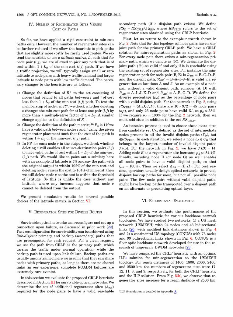
In this section, we evaluate the performance of theproposed CRLP heuristic for various backbone networktopologies. We have studied two networks: 1) a US meshnetwork (USMESH) with 24 nodes and 43 bidirectionallinks [20] with modified link distances shown in Fig. 4and 2) a continental US topology (CONUS) with 75 nodesand 99 bidirectional links shown in Fig. 6. CONUS is afiber-optic backbone network developed for use in the re-search of large-scale DWDM networks [23].

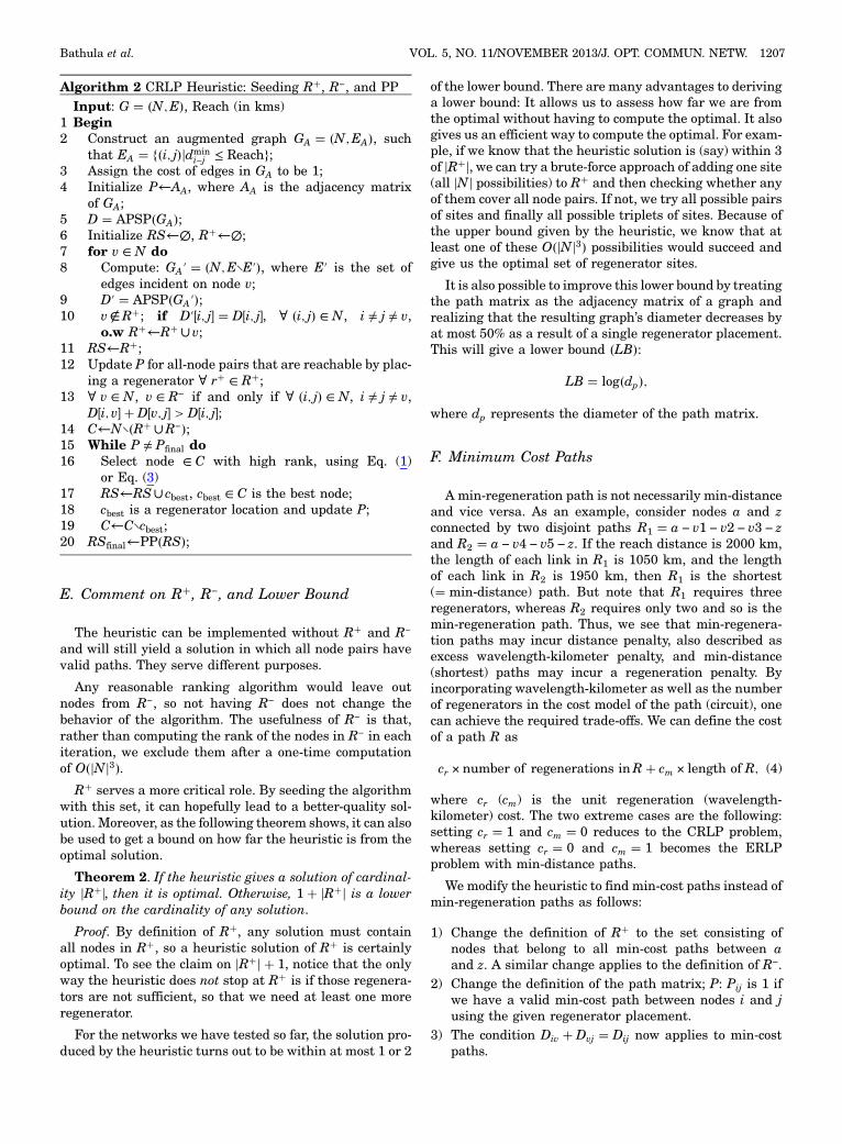
We have compared the CRLP heuristic with an optimalILP1 solution for min-regeneration on the USMESHtopology. For reach distances of 1400, 1800, 2000, 2400,and 2500 km, the numbers of regenerator sites were 17,12, 11, 8, and 9, respectively, for both the CRLP heuristicand the ILP solution. From Fig. 5(b), we observe that re-generator sites increase for a reach distance of 2500 km.

1ILP formulation is detailed in Appendix A.


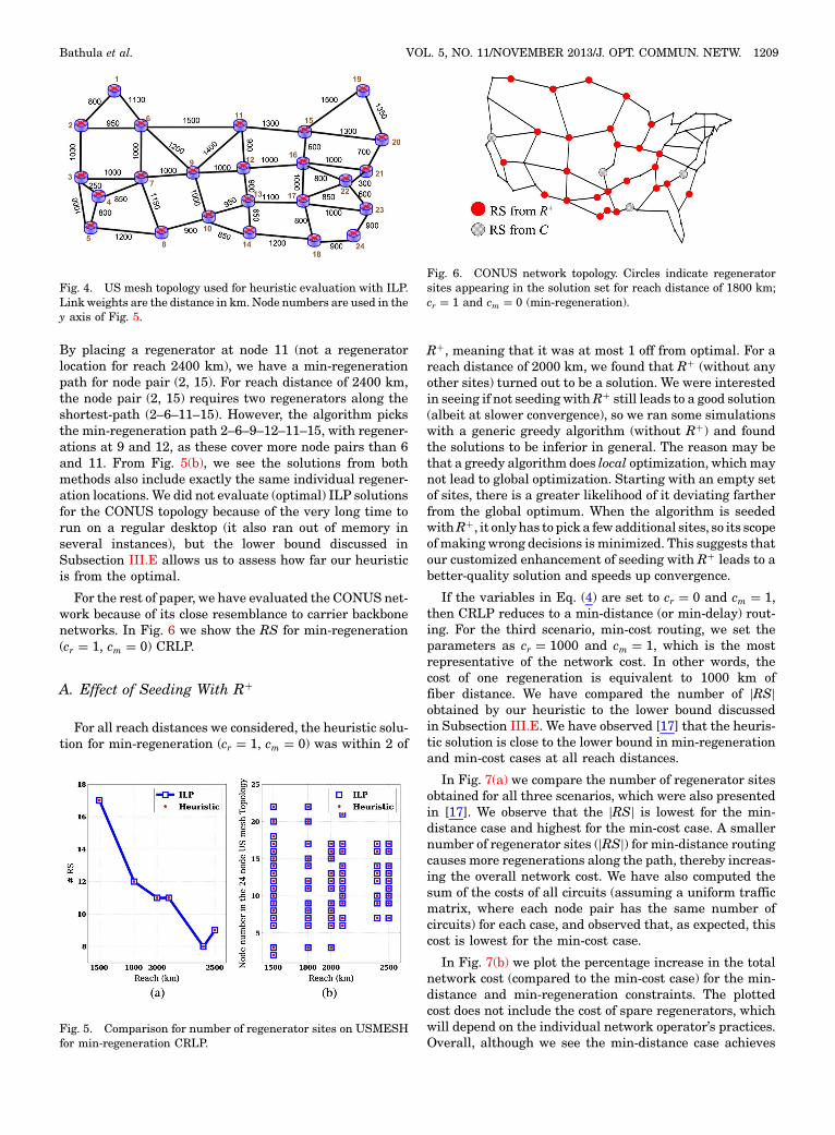
By placing a regenerator at node 11 (not a regeneratorlocation for reach 2400 km), we have a min-regenerationpath for node pair (2, 15). For reach distance of 2400 km,the node pair (2, 15) requires two regenerators along theshortest-path (2–6–11–15). However, the algorithm picksthe min-regeneration path 2–6–9–12–11–15, with regener-ations at 9 and 12, as these cover more node pairs than 6and 11. From Fig. 5(b), we see the solutions from bothmethods also include exactly the same individual regener-ation locations. We did not evaluate (optimal) ILP solutionsfor the CONUS topology because of the very long time torun on a regular desktop (it also ran out of memory inseveral instances), but the lower bound discussed inSubsection III.E allows us to assess how far our heuristicis from the optimal.

For the rest of paper, we have evaluated the CONUS net-work because of its close resemblance to carrier backbonenetworks. In Fig. 6 we show the RS for min-regeneration(cr � 1, cm � 0) CRLP.

A. Effect of Seeding With R�

For all reach distances we considered, the heuristic solu-tion for min-regeneration (cr � 1, cm � 0) was within 2 of

R�, meaning that it was at most 1 off from optimal. For areach distance of 2000 km, we found that R� (without anyother sites) turned out to be a solution. We were interestedin seeing if not seeding withR� still leads to a good solution(albeit at slower convergence), so we ran some simulationswith a generic greedy algorithm (without R�) and foundthe solutions to be inferior in general. The reason may bethat a greedy algorithm does local optimization, which maynot lead to global optimization. Starting with an empty setof sites, there is a greater likelihood of it deviating fartherfrom the global optimum. When the algorithm is seededwithR�, it only has to pick a fewadditional sites, so its scopeof making wrong decisions is minimized. This suggests thatour customized enhancement of seeding with R� leads to abetter-quality solution and speeds up convergence.

If the variables in Eq. (4) are set to cr � 0 and cm � 1,then CRLP reduces to a min-distance (or min-delay) rout-ing. For the third scenario, min-cost routing, we set theparameters as cr � 1000 and cm � 1, which is the mostrepresentative of the network cost. In other words, thecost of one regeneration is equivalent to 1000 km offiber distance. We have compared the number of jRSjobtained by our heuristic to the lower bound discussedin Subsection III.E. We have observed [17] that the heuris-tic solution is close to the lower bound in min-regenerationand min-cost cases at all reach distances.

In Fig. 7(a) we compare the number of regenerator sitesobtained for all three scenarios, which were also presentedin [17]. We observe that the jRSj is lowest for the min-distance case and highest for the min-cost case. A smallernumber of regenerator sites (jRSj) for min-distance routingcauses more regenerations along the path, thereby increas-ing the overall network cost. We have also computed thesum of the costs of all circuits (assuming a uniform trafficmatrix, where each node pair has the same number ofcircuits) for each case, and observed that, as expected, thiscost is lowest for the min-cost case.

In Fig. 7(b) we plot the percentage increase in the totalnetwork cost (compared to the min-cost case) for the min-distance and min-regeneration constraints. The plottedcost does not include the cost of spare regenerators, whichwill depend on the individual network operator’s practices.Overall, although we see the min-distance case achieves

Fig. 6. CONUS network topology. Circles indicate regeneratorsites appearing in the solution set for reach distance of 1800 km;cr � 1 and cm � 0 (min-regeneration).

Fig. 5. Comparison for number of regenerator sites on USMESHfor min-regeneration CRLP.

Fig. 4. US mesh topology used for heuristic evaluation with ILP.Link weights are the distance in km. Node numbers are used in they axis of Fig. 5.


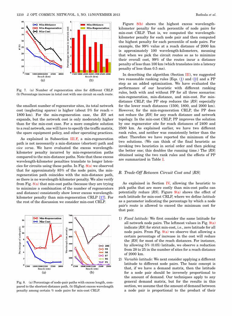
the smallest number of regenerator sites, its total networkcost (neglecting spares) is higher (about 5% for reach �1800 km). For the min-regeneration case, the RS setexpands, but the network cost is only moderately higherthan for the min-cost case. For a more complete solutionto a real network, one will have to specify the traffic matrix,the spare equipment policy, and other operating practices.

As explained in Subsection III.F, a min-regenerationpath is not necessarily a min-distance (shortest) path andvice versa. We have evaluated the excess wavelength-kilometer penalty incurred by min-regeneration pathscompared to themin-distance paths. Note that these excesswavelength-kilometer penalties translate to longer laten-cies for circuits using these paths. In Fig. 8(a) we observedthat for approximately 85% of the node pairs, the min-regeneration path coincides with the min-distance path,so there is no wavelength-kilometer penalty. We also verifyfrom Fig. 8(a) that min-cost paths (because they are tryingto minimize a combination of the number of regeneratorsand distance) consistently show lower excess wavelength-kilometer penalty than min-regeneration CRLP [17]. Forthe rest of the discussion we consider min-cost CRLP.

Figure 8(b) shows the highest excess wavelength-kilometer penalty for each percentile of node pairs formin-cost CRLP. That is, we computed the wavelength-kilometer penalty for each node pair and then computedthe highest penalty for each percentile of node pairs. Forexample, the 99% value at a reach distance of 2000 kmis approximately 100 wavelength-kilometers, meaningthat when we pick the circuit routes so as to minimizetheir overall cost, 99% of the routes incur a distancepenalty of less than 100 km (which translates into a latencypenalty of less than 0.5 ms).

In describing the algorithm (Section III), we suggestedtwo reasonable ranking rules [Eqs. (1) and (3)] and a PPstep as an added optimization. We have evaluated theperformance of our heuristic with different rankingrules, both with and without PP for all three scenarios:min-regeneration, min-distance, and min-cost. For min-distance CRLP, the PP step reduces the jRSj especiallyfor the lower reach distances (1500, 1800, and 2000 km).However, for the min-regeneration CRLP, the PP doesnot reduce the jRSj for any reach distance and networktopology. In the min-cost CRLP, PP improves the solutionby one regenerator site for reach distances of 2400 and2500 km. As explained earlier, we have two differentrank rules, and neither was consistently better than theother. Therefore we have reported the minimum of thetwo solutions. (We can think of the final heuristic asinvoking two heuristics in serial order and then pickingthe better one; this doubles the running time.) The jRSjobtained using the two rank rules and the effects of PPare summarized in Table I.

B. Trade-Off Between Circuit Cost and jRSj

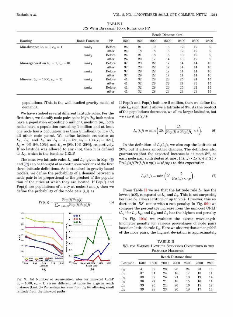
As explained in Section IV, allowing the heuristic topick paths that are more costly than min-cost paths canpotentially reduce jRSj. Figure 9(a) shows the effect ofsuch latitude for min-cost CRLP, where we define latitudeas a parameter indicating the percentage by which a nodepair’s route is allowed to exceed the minimum cost forthat pair.

1) Fixed latitude: We first consider the same latitude forall network node pairs. The leftmost values in Fig. 9(a)indicate jRSj for strict min-cost, i.e., zero latitude for allnode pairs. From Fig. 9(a) we observe that allowing acertain percentage of increase in the cost will reducethe jRSj for most of the reach distances. For instance,by allowing 5% (0.05) latitude, we observe a reductionfrom 28 to 25 in the number of sites for a reach distanceof 2000 km.

2) Variable latitude:We next consider applying a differentlatitude to different node pairs. The basic concept isthat, if we have a demand matrix, then the latitudefor a node pair should be inversely proportional tothe amount of demand. Our techniques apply to anygeneral demand matrix, but for the results in thissection, we assume that the amount of demand betweena node pair is proportional to the product of their

Fig. 8. (a) Percentage of node-pair paths with excess length, com-pared to the shortest-distance path. (b) Highest excess wavelengthpenalty among certain % node pairs for min-cost CRLP.

Fig. 7. (a) Number of regeneration sites for different CRLP.(b) Percentage increase in total cost with one circuit on each route.


populations. (This is the well-studied gravity model ofdemand).

We have studied several different latitude rules. For thefirst three, we classify node pairs to be high (hi, both nodeshave a population exceeding 5 million), medium (mi, bothnodes have a population exceeding 1 million and at leastone node has a population less than 5 million), or low (li,all other node pairs). We define latitude scenarios asL1, L2, and L3 as L1 � �h1 � 5%;m1 � 10%; l1 � 15%�,L2 � �0%; 5%;10%�, and L3 � �0%; 10%; 25%�, respectively.If no latitude was allowed to any �np�, then it is definedas L0, which is the baseline CRLP.

The next two latitude rules L4 and L5 [given in Eqs. (6)and (7)] can be thought of as continuous versions of the firstthree latitude definitions. As is standard in gravity-basedmodels, we define the probability of a demand between anode pair to be proportional to the product of the popula-tion of the cities at which they are located. If Pop�i� andPop� j� are populations of a city at nodes i and j, then wedefine the probability of the node pair �i; j� as

Pr�i; j� � Pop�i�Pop�j�P∀ �i;j�;i≠jPop�i�Pop� j�

: (5)

If Pop�i� and Pop�j� both are 5 million, then we define therule L4 such that it allows a latitude of 3%. As the productof the populations decreases, we allow larger latitudes, butwe cap it at 20%.

L4�i; j� � min�20; ⌊ 25

Pop�i� × Pop� j�⌋ × 3�: (6)

In the definition of L5�i; j�, we also cap the latitude at20%, but it allows smoother changes. The definition alsoguarantees that the expected increase is at most 5%, aseach node pair contributes at most Pr�i; j� × L5�i; j� ≤ ��5 ×Pr�i; j��∕�Pr�i; j� × np�� 5∕np� to this expectation.

L5�i; j� � min�20;

5Pr�i; j� × np

�: (7)

From Table II we see that the latitude rule L3 has thelowest jRSj, compared to L1 and L2. This is not surprisingbecause L3 allows latitude of up to 25%. However, this re-duction in jRSj comes with a cost penalty. In Fig. 9(b) wecompare the percentage increase from the min-cost CRLP(L0) for L1, L2, and L3, and L3 has the highest cost penalty.

In Fig. 10(a) we evaluate the excess wavelength-kilometer penalty for various percentages of node pairsbased on latitude rule L3. Here we observe that among 99%of the node pairs, the highest deviation is approximately

Fig. 9. (a) Number of regeneration sites for min-cost CRLP(cr � 1000, cm � 1) versus different latitudes for a given reachdistance (km). (b) Percentage increase from L0 for allowing smalllatitude from the min-cost paths.

TABLE IIjRSj FOR VARIOUS LATITUDE SCENARIOS CONSIDERED IN THE

PROPOSED HEURISTIC

Reach Distance (km)

Latitude 1500 1800 2000 2200 2400 2500 2800

L0 41 32 28 23 24 23 15L1 37 31 24 18 17 18 11L2 38 32 24 21 18 19 14L3 36 27 21 18 15 16 11L4 39 26 21 20 16 15 12L5 39 28 23 20 18 17 14

TABLE IRS WITH DIFFERENT RANK RULES AND PP

Reach Distance (km)

Routing Rank Function PP 1500 1800 2000 2200 2400 2500 2800

Min-distance (cr � 0, cm � 1) rank1 Before 25 21 19 15 12 12 9After 24 18 18 15 12 12 9

rank2 Before 24 21 18 15 13 12 9After 24 20 17 14 13 12 9

Min-regeneration (cr � 1, cm � 0) rank1 Before 37 29 22 17 14 14 10After 37 29 22 17 14 14 10


Min-cost (cr � 1000, cm � 1) rank1 Before 41 32 28 23 25 24 15After 41 32 28 23 24 23 15



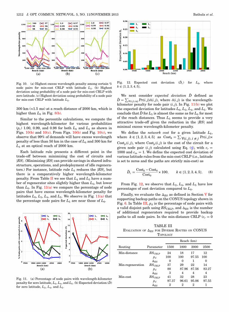
300 km (≈1.5 ms) at a reach distance of 2000 km, which ishigher than L0 in Fig. 8(b).

Similar to the percentile calculations, we compute thehighest wavelength-kilometer for various probabilities(pr) 1.00, 0.99, and 0.98 for both L0 and L3 as shown inFigs. 10(b) and 10(c). From Figs. 10(b) and Fig. 10(c), weobserve that 99% of demands will have excess wavelengthpenalty of less than 50 km in the case of L0 and 300 km forL3 at an optical reach of 2000 km.

Each latitude rule presents a different point in thetrade-off between minimizing the cost of circuits andjRSj. (Minimizing jRSj can provide savings in shared infra-structure, operations, and predeployment of idle regenera-tors.) For instance, latitude rule L3 reduces the jRSj, butthere is a comparatively higher wavelength-kilometerpenalty. From Table II we see that L4 and L5 have a num-ber of regenerator sites slightly higher than L3, but lowerthan L0. In Fig. 11(a) we compare the percentage of nodepairs that have excess wavelength-kilometer penalty forlatitudes L0, L3, L4, and L5. We observe in Fig. 11(a) thatthe percentage node pairs for L5 are near those of L0.

We next consider expected deviation D̄ defined asD̄ � P

∀�i;j�;i≠j Pr�i; j�δ�i; j�, where δ�i; j� is the wavelength-kilometer penalty for node pair �i; j�. In Fig. 11(b) we plotthe expected deviation for latitudes L0, L3, L4, and L5. Weconclude that D̄ for L5 is almost the same as for L0 for mostof the reach distances. Thus L5 seems to provide a veryattractive trade-off given the reduction in the jRSj andminimal excess wavelength-kilometer penalty.

We define the network cost for a given latitude Lk,where k ∈ f1;2;3;4; 5g as Costk � P

∀�i; j�; i ≠ j Pr�i; j�×Costp�i; j�, where Costp�i; j� is the cost of the circuit for agiven node pair �i; j� calculated using Eq. (4), with cr �1000 and cm � 1. We define the expected cost deviation ofvarious latitude rules from themin-cost CRLP (i.e., latitudeis set to zeros and the paths are strictly min-cost) as

D̄c �Costk − Cost0

Cost0× 100; k ∈ f1; 2; 3; 4; 5g: (8)

From Fig. 12, we observe that L2, L4, and L5 have lowpercentages of cost deviation compared to L0.

Finally, we evaluate the ΔRS as defined in Section V forsupporting backup paths on the CONUS topology shown inFig. 6. In Table III, pd is the percentage of node pairs witha valid disjoint path using RSCRLP, and ΔRS is the numberof additional regenerators required to provide backuppaths to all node pairs. In the min-distance CRLP (cr � 0

Fig. 10. (a) Highest excess wavelength penalty among certain %node pairs for min-cost CRLP with latitude L3. (b) Highestdeviation using probability of a node pair for min-cost CRLP withzero latitude. (c) Highest deviation using probability of a node pairfor min-cost CRLP with latitude L3.

Fig. 11. (a) Percentage of node pairs with wavelength-kilometerpenalty for zero latitude, L3, L4, and L5. (b) Expected deviation (D̄)for zero latitude, L3, L4, and L5.

Fig. 12. Expected cost deviation (D̄c) for Lk, wherek ∈ f1; 2;3; 4; 5g.

TABLE IIIEVALUATION OF ΔRS FOR DIVERSE ROUTES ON CONUS

TOPOLOGY

Reach (km)

Routing Parameter 1500 1800 2000 2500

Min-distance RSCRLP 24 18 17 12pd 100 100 97.55 100ΔRS 0 0 1 0

Min-regeneration RSCRLP 37 29 22 14pd 88 87.96 87.56 83.27ΔRS 3 4 4 4

Min-cost RSCRLP 41 32 28 23pd 97.37 96.61 95.06 97.55ΔRS 2 2 2 1


and cm � 1), we find that using RSCRLP, all node pairs havea valid disjoint path, i.e., pd � 100%, and henceΔRS � 0 formost of the reach distances. For min-regeneration (cr � 1and cm � 0) and min-cost (cr � 1000 and cm � 0) CRLP,ΔRS ≠ 0.

VII. CONCLUSION

To plan predeployment of regenerators effectively inpractical networks, we have introduced a constrained rout-ing regenerator location problem and presented a heuristicapproach to address it. Unlike previous research work onregenerator placement, we pursue a holistic approach ofminimizing overall network cost by considering acombination of the number of regenerators used and thewavelength-kilometer of individual circuits, as well as theprobability of demand between each node pair and the num-ber of sites.We start with a basic heuristic and then presentvarious enhancements that refine the trade-off between thenumber of sites and the cost of individual circuits. The heu-ristic also constructs a lower bound, thus letting us evaluatehowcloselyweapproach the optimal.Extensive simulationson large topologies show that the heuristic achieves near-optimal results. Our heuristic algorithm can be easily tunedfor practical ROADM networks where instead of a fixedreach distance, a reach table is used to specify all reachablepaths in the network (such tables are generated by a ven-dor’s planning tools using detailed network information).Finally our experiments indicate that a small additionalnumber of regenerator sites allow survivable connectionsbetween most node pairs. We further plan to extend thiswork to evaluate 1) the usage of regenerators at each se-lected site for dynamic traffic and 2) complex requirementsof disjointness on connection between multiple node pairs.

APPENDIX A

In this appendix, we present the ILP formulations forthe proposed CRLP. Given the original graph G � �N;E�with a set of N vertices and a set of E edges, we constructan augmented graph GA � �N;EA�, such that we add anedge between two nodes if they are within the reach dis-tance, where EA represents the set of augmented edges.

A. Notations

• role�u� � 1 if regenerators are placed in u, 0 otherwise.• K: the set of connection requests in the traffic matrix.• src�k�: the source node of the kth request.• tgt�k�: the destination node of the kth request.• f ku;v: if the link �u; v� is used for the kth request, the valueis 1. Otherwise, the value is 0.

• out�u�: the outgoing adjacent node set of node u.• in�u�: the incoming adjacent node set of node u.• jNj: the number of nodes in the network graph, where Nis the set of nodes.

• Hk: given hops on request k.

B. CRLP Formulation

Objective

minXu∈V

role�u�: (A1)

Constraints

X�u;v�∈E

f ku;v � Hk; ∀ k ∈ K; (A2)

Xv∈out�s�

f ks;v −X

v∈in�s�f kv;s � 1; ∀ k ∈ K; s � src�k�; (A3)

Xv∈in�t�

f kv;t −X

v∈out�t�f kt;v � 1; ∀ k ∈ K; t � tgt�k�; (A4)

Xv∈out�u�

f ku;v �X

v∈in�u�f kv;u;

∀ k ∈ K; ∀ u ∈ V�≠ src�k� or tgt�k��; (A5)

role�u� ≥P

v∈out�u�fku;v

N;

∀ k ∈ K; ∀ u ∈ V�≠ src�k� or tgt�k��;f ku;v; role�u� ∈ f0;1g: (A6)

In the CRLP problem, we can select a path from all theroutes that use theminimum number of regenerations. Thepaths that use the minimum number of regenerations arethe shortest paths (in terms of path hops) in our newly gen-erated graph GA. In Eq. (A5), Hk is the number of hops ofthe shortest path for connection k in GA. Equation (A2)makes sure that the number of links used on the connectionequals the number of hops of the shortest path. By doingthis, we guarantee that a path with minimum regenerationwill be selected.

Constraints (A3)–(A5) are the flow conservation con-straints for all connection requests. In constraint (A6),for a node u, which is used as the intermediate node forsome connection, it will be a regeneration node.

ACKNOWLEDGMENTS

The authors acknowledge many useful suggestions andcomments from D. Xu and G. Zussman and support fromthe CIAN NSF ERC (subaward Y503160). This paperwas presented in parts at DRCN 2013 [18] and OFC/NFOEC 2012 [17].

REFERENCES

[1] A. Gerber and R. Doverspike, “Traffic types and growth inbackbone networks,” in Nat. Fiber Optic Engineers Conf.,Los Angeles, CA, Mar. 2011, pp. 1–3.


[2] J. Simmons, E. L. Goldstein, and A. A.M. Saleh, “On the valueof wavelength-add/drop in WDM rings with uniform traffic,”in Nat. Fiber Optic Engineers Conf., San Jose, CA, Feb. 1998,pp. 361–362.

[3] W. Van Parys, P. Arijs, O. Antonis, and P. Demeester, “Quan-tifying the benefits of selective wavelength regeneration inultra long-haul WDM networks,” in Optical Fiber Communi-cation Conf. and Exhibit, Anaheim, CA, Mar. 2001, vol. 2,paper TuT4.

[4] M. D. Feuer, D. C. Kilper, and S. L. Woodward, “ROADMs andtheir system applications,” in Optical Fiber Telecommunica-tions. Waltham, MA: Academic, 2008, pp. 293–343.

[5] A. A. Mahimkar, A. Chiu, R. Doverspike, M. Feuer, P. Magill,E. Mavrogiorgis, J. Pastor, V. Sethi, D. Xu, S. Woodward, andJ. Yates, “Outage detection and dynamic re-provisioning inGRIPhoN: A globally reconfigurable intelligent photonic net-work,” in Nat. Fiber Optic Engineers Conf., Los Angeles, CA,Mar. 2012, paper NM2F.5.

[6] S. Woodward, M. Feuer, I. Kim, P. Palacharla, X. Wang, and D.Bihon, “Service velocity: Rapid provisioning strategies inoptical ROADM networks,” J. Opt. Commun. Netw., vol. 4,no. 2, pp. 92–98, Feb. 2012.

[7] X. Zhang, M. Birk, A. Chiu, R. Doverspike,M. Feuer, P. Magill,E. Mavrogiorgis, J. Pastor, S. Woodward, and J. Yates,“Bridge-and-roll demonstration in GRIPhoN (Globally Recon-figurable Intelligent Photonic Network),” in Nat. Fiber OpticEngineers Conf., San Diego, CA, Mar. 2010, pp. 1–3.

[8] A. Chiu, G. Choudhury, G. Clapp, R. Doverspike, M. Feuer, J.Gannett, J. Jackel, G. Kim, J. Klincewicz, T. Kwon, G. Li, P.Magill, J. Simmons, R. Skoog, J. Strand, A. Lehmen, B.Wilson, S. Woodward, and D. Xu, “Architectures and protocolsfor capacity efficient, highly dynamic and highly resilient corenetworks [Invited],” J. Opt. Commun. Netw., vol. 4, no. 1,pp. 1–14, Jan. 2012.

[9] M. Feuer, S. Woodward, I. Kim, P. Palacharla, X. Wang, D.Bihon, B. Bathula, W. Zhang, R. Sinha, G. Li, and A. Chiu,“Simulations of a service velocity network employing regen-erator site concentration,” in Nat. Fiber Optic EngineersConf., Los Angeles, CA, Mar. 2012, paper NTu2J.5.

[10] M. Flammini, A. Marchetti-Spaccamela, G. Monaco, L.Moscardelli, and S. Zaks, “On the complexity of the regener-ator placement problem in optical networks,” in Proc. 2ndAnnu. Symp. Parallelism Algorithms and Architectures(SPAA), 2009, pp. 154–162.

[11] S. Chen, I. Ljubic, and S. Raghavan, “The generalized regen-erator location problem,” in Proc. Int. Network OptimizationConf., 2009, pp. 1–32.

[12] S. Chen, I. Ljubic, and S. Raghavan, “The regenerator place-ment problem,” Networks, vol. 55, no. 3, pp. 205–220, 2010.

[13] A. Duarte, R. Martí, andM. G. C. Resende, “Randomized heu-ristics for the regenerator location problem,” OptimizationOnline, 2010. [Online]. Available: http://www.optimization‑online.org/DB_HTML/2010/08/2706.html.

[14] M. Flammini, A. Marchetti-Spaccamela, G. Monaco, L.Moscardelli, and S. Zaks, “On the complexity of the regener-ator placement problem in optical networks,” IEEE/ACMTrans. Netw., vol. 19, no. 2, pp. 498–511, Apr. 2011.

[15] G. Shen, W. Grover, T. Cheng, and S. Bose, “Sparse placementof electronic switching nodes for low blocking in translucentoptical networks,” J. Opt. Netw., vol. 1, no. 12, pp. 424–441,Dec. 2002.

[16] X. Yang and B. Ramamurthy, “Sparse regeneration in trans-lucent wavelength-routed optical networks: Architecture,network design and wavelength routing,” Photon. Netw.Commun., vol. 10, pp. 39–53, July 2005.

[17] B. G. Bathula, R. Sinha, A. Chiu, M. Feuer, G. Li, S.Woodward, W. Zhang, K. Bergman, I. Kim, and P. Palacharla,“On concentrating regenerator sites in ROADM networks,”in Nat. Fiber Optic Engineers Conf., Los Angeles, CA,Mar. 2012, paper NW3F.6.

[18] B. G. Bathula, R. K. Sinha, A. L. Chiu, M. D. Feuer, G. Li,S. L. Woodward, W. Zhang, R. Doverspike, P. Magill, andK. Bergman, “Cost optimization using regenerator siteconcentration and routing in ROADM networks [Invited],”in 9th Int. Conf. Design of Reliable Communication Networks(DRCN), Budapest, Hungary, Mar. 2013, pp. 139–147.

[19] M. Garey and D. S. Johnson, Computers and Intractability: AGuide to the Theory of NP-Completeness. W. H. Freeman andCompany, 1979.

[20] S. Rai, C. F. Su, and B. Mukherjee, “On provisioning inall-optical networks: An impairment-aware approach,”IEEE/ACM Trans. Netw., vol. 17, no. 6, pp. 1989–2001,Dec. 2009.

[21] C. Gao, H. Cankaya, A. Patel, J. Jue, X. Wang, Q. Zhang, P.Palacharla, and M. Sekiya, “Survivable impairment-awaretraffic grooming and regenerator placement with connection-level protection,” J. Opt. Commun. Netw., vol. 4, no. 3,pp. 259–270, Mar. 2012.

[22] X. Yang, L. Shen, and B. Ramamurthy, “Survivable lightpathprovisioning in WDM mesh networks under shared pathprotection and signal quality constraints,” J. LightwaveTechnol., vol. 23, no. 4, pp. 1556–1567, Apr. 2005.

[23] A. Chiu, G. Choudhury, G. Clapp, R. Doverspike, J. Gannett, J.Klincewicz, G. Li, R. Skoog, J. Strand, A. Von Lehmen, and D.Xu, “Network design and architectures for highly dynamicnext-generation IP-over-optical long distance networks,”J. Lightwave Technol., vol. 27, no. 12, pp. 1878–1890,June 2009.


http://www.optimization-online.org/DB_HTML/2010/08/2706.html





Documents

Constraint Routing and Regenerator Site Concentration in ...lightwave.ee.columbia.edu/Publications/Bathula2013.pdf · Constraint Routing and Regenerator Site Concentration in ROADM