Embed Size (px)
Citation preview

Constraints and Collisions
Steve Rotenberg CSE291: Physics Simulation
UCSD Spring 2019
Rotational Inertia
• The rotational inertia tensor 𝐈 is a 3x3 symmetric matrix that is essentially the rotational equivalent of mass
• It relates the angular momentum 𝐋 of a rigid body to its angular velocity 𝛚 by the equation
𝐋 = 𝐈 ⋅ 𝛚
• This is similar to how mass relates linear momentum to
linear velocity with 𝐩 = 𝑚𝐯, but adds additional complexity because 𝐈 is not only a matrix instead of a scalar, but it also changes over time as the object rotates
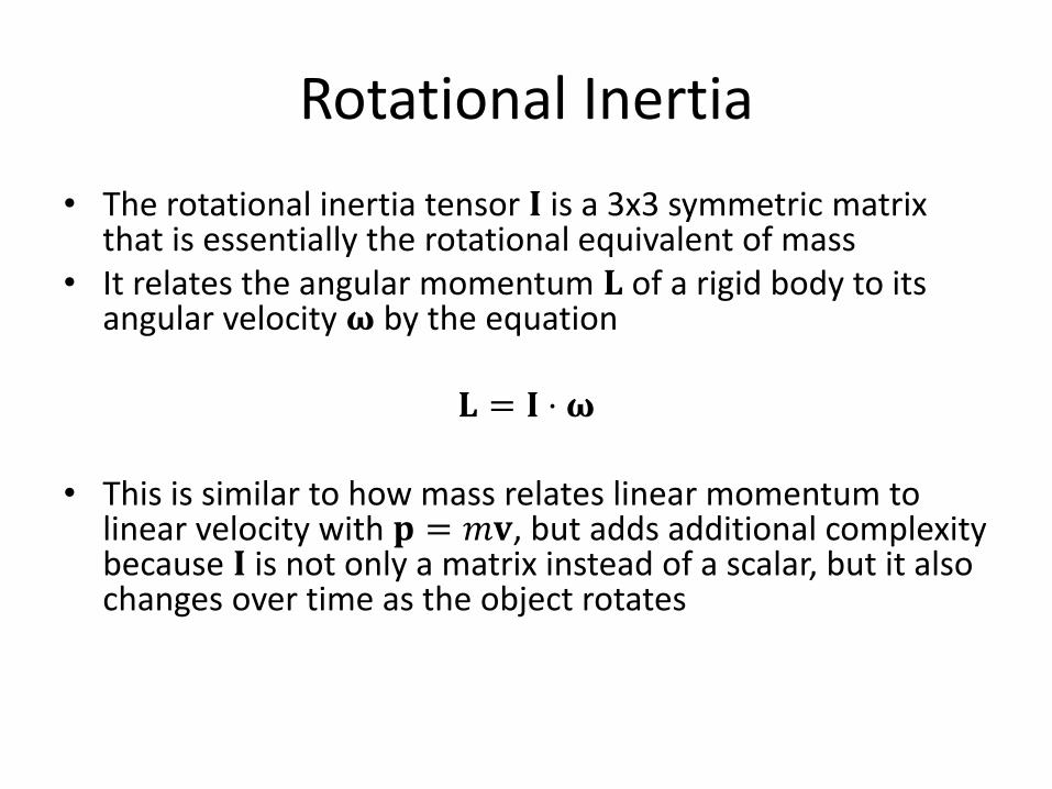
Principal Axes & Inertias
• If we diagonalize the 𝐈 matrix, we get an orientation matrix 𝐀 and a constant diagonal matrix 𝐈0
𝐈 = 𝐀 ⋅ 𝐈0 ⋅ 𝐀𝑇
• The matrix 𝐀 rotates the object from an orientation where the principal axes line up with the x, y, and z axes
• The three diagonal values in 𝐈0, (namely 𝐼𝑥, 𝐼𝑦, and 𝐼𝑧) are the principal inertias. They represent the resistance to torque around the corresponding principal axis (in a similar way that mass represents the resistance to force)

Rigid Body Dynamics
• The center of mass of a rigid body behaves like a particle: – Position: 𝐱
– Velocity: 𝐯 =𝑑𝐱
𝑑𝑡
– Acceleration: 𝐚 =𝑑𝐯
𝑑𝑡=
𝑑2𝐱
𝑑𝑡2
– Mass: 𝑚
– Momentum: 𝐩 = 𝑚𝐯
– Force: 𝐟 =𝑑𝐩
𝑑𝑡= 𝑚𝐚

Rigid Body Dynamics
• Rigid bodies have additional properties for rotation: – Orientation: 𝐀
– Angular velocity: 𝛚
– Angular acceleration: 𝛚 =𝑑𝛚
𝑑𝑡
– Rotational inertia: 𝐈 = 𝐀 ⋅ 𝐈0 ⋅ 𝐀𝑇
– Angular momentum: 𝐋 = 𝐈 ⋅ 𝛚
– Torque: 𝛕 =𝑑𝐋
𝑑𝑡= 𝛚× 𝐈 ⋅ 𝛚 + 𝐈 ⋅ 𝛚

Applied Forces
• When we apply a force to a rigid body at some position 𝐱𝑟, this is equivalent to applying the same force on the center of mass as well as a torque equal to 𝐫 × 𝐟, where 𝐫 = 𝐱𝑟 − 𝐱 and 𝐱 is the position of the center of mass of the rigid body
• Various forces can apply to a rigid body and they are just summed up as a single total force and torque:
𝐟𝑡𝑜𝑡𝑎𝑙 = 𝐟𝑖
𝛕𝑡𝑜𝑡𝑎𝑙 = 𝐫𝑖 × 𝐟𝑖
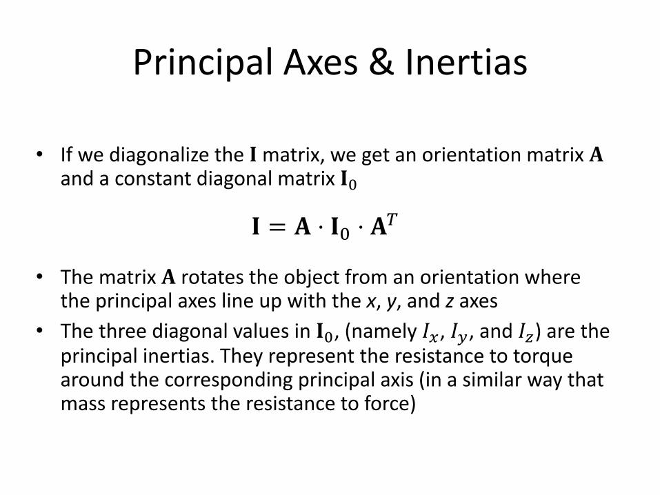
Newton-Euler Equations
• The Newton-Euler equations describe the motion of a rigid body under applied force and torque:
𝐟 = 𝑚𝐚 𝛕 = 𝛚 × 𝐈 ⋅ 𝛚 + 𝐈 ⋅ 𝛚 • Solved for acceleration: 𝐚 = 𝐟 𝑚 𝛚 = 𝐈−1 𝛕 − 𝛚 × 𝐈 ⋅ 𝛚
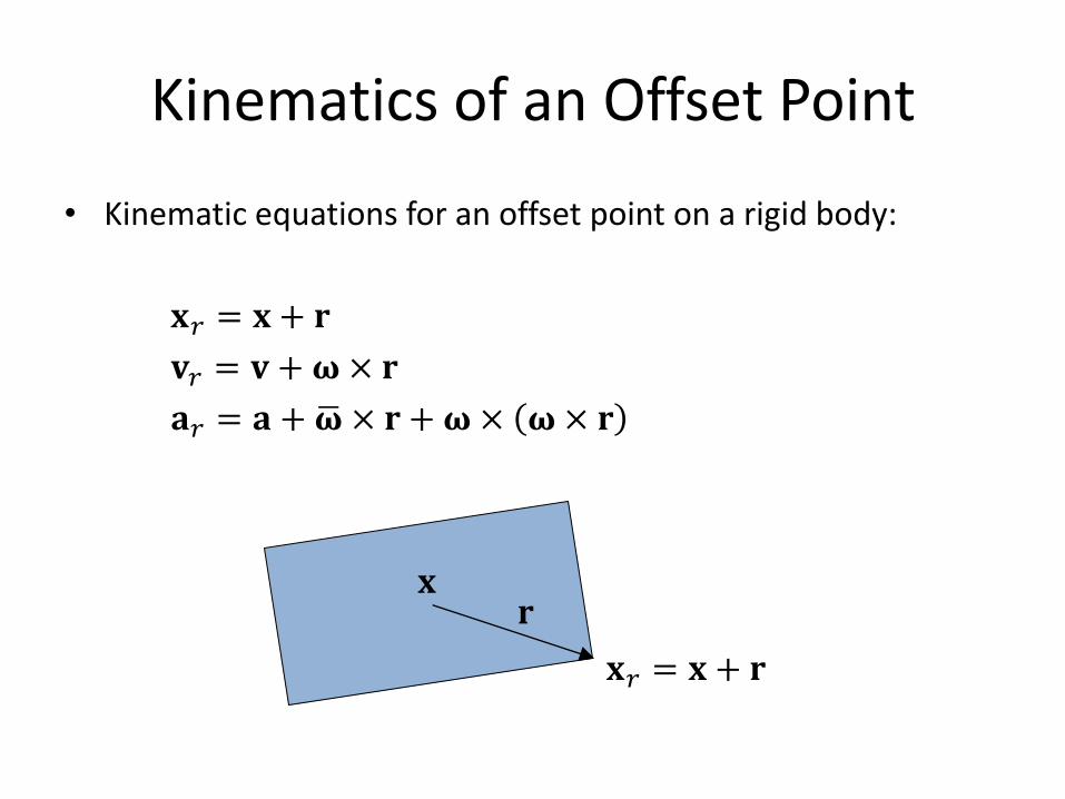
Kinematics of an Offset Point
• Kinematic equations for an offset point on a rigid body:
𝐱𝑟 = 𝐱 + 𝐫
𝐯𝑟 = 𝐯 +𝛚 × 𝐫
𝐚𝑟 = 𝐚 +𝛚 × 𝐫 +𝛚 × 𝛚× 𝐫
𝐱 𝐫
𝐱𝑟 = 𝐱 + 𝐫
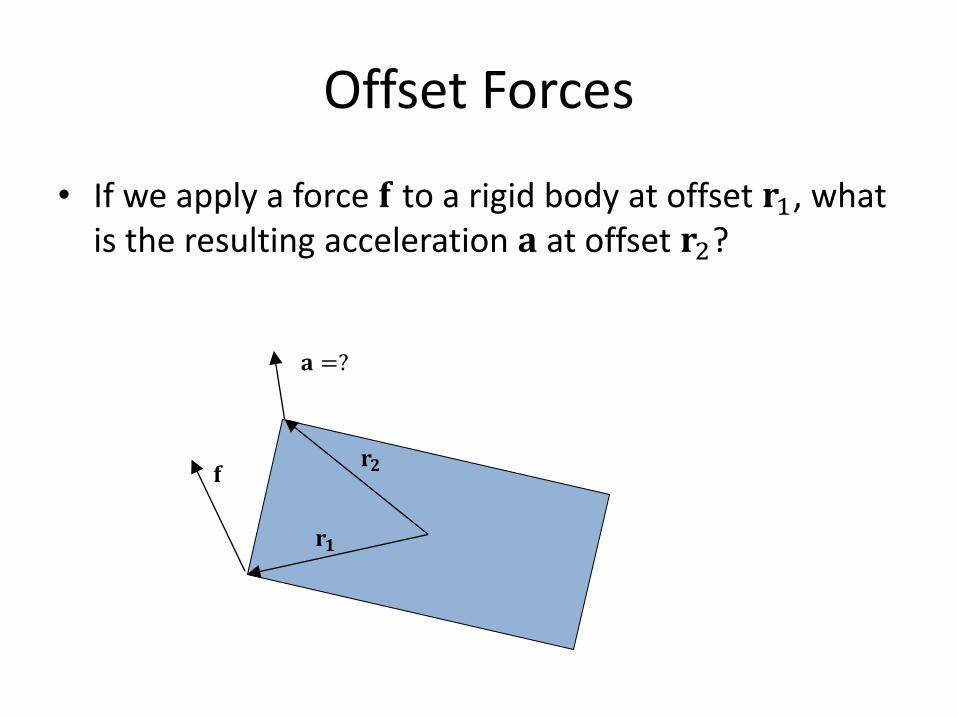
Offset Forces
• If we apply a force 𝐟 to a rigid body at offset 𝐫1, what is the resulting acceleration 𝐚 at offset 𝐫2?
𝐟
𝐚 =?
𝐫𝟏
𝐫𝟐
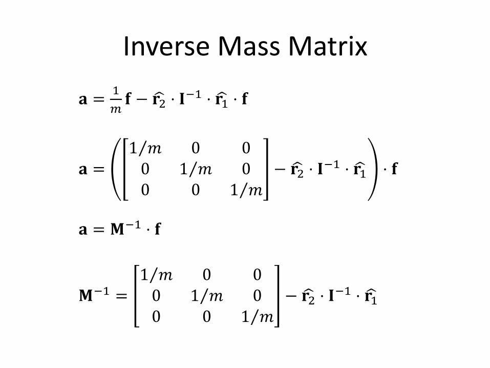
Inverse Mass Matrix
𝐚 =1
𝑚𝐟 − 𝐫2 ⋅ 𝐈−1 ⋅ 𝐫1 ⋅ 𝐟
𝐚 =1 𝑚 0 00 1 𝑚 00 0 1 𝑚
− 𝐫2 ⋅ 𝐈−1 ⋅ 𝐫1 ⋅ 𝐟
𝐚 = 𝐌−1 ⋅ 𝐟
𝐌−1 =1 𝑚 0 00 1 𝑚 00 0 1 𝑚
− 𝐫2 ⋅ 𝐈−1 ⋅ 𝐫1

Rigid Pendulum
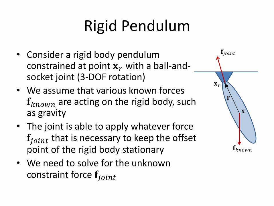
Rigid Pendulum
• Consider a rigid body pendulum constrained at point 𝐱𝑟 with a ball-and-socket joint (3-DOF rotation)
• We assume that various known forces 𝐟𝑘𝑛𝑜𝑤𝑛 are acting on the rigid body, such as gravity
• The joint is able to apply whatever force 𝐟𝑗𝑜𝑖𝑛𝑡 that is necessary to keep the offset point of the rigid body stationary
• We need to solve for the unknown constraint force 𝐟𝑗𝑜𝑖𝑛𝑡
𝐱𝑟
𝐫
𝐱
𝐟𝑘𝑛𝑜𝑤𝑛
𝐟𝑗𝑜𝑖𝑛𝑡

Rigid Pendulum
• To evaluate all forces at a particular instant:
– We first evaluate all known forces on the rigid body (gravity, air friction, joint friction, etc.)
– Next, we can determine what the acceleration 𝐚𝑟 of the offset point 𝐱𝑟 would be with no constraint
– Then, we can use the inverse mass matrix to solve for the joint force needed to counteract the acceleration and hold the joint together

Offset Acceleration
• Assuming a known total force 𝐟𝑘𝑛𝑜𝑤𝑛 and torque 𝛕𝑘𝑛𝑜𝑤𝑛 are acting on the rigid body, we can calculate the acceleration 𝐚𝑟 at relative offset 𝐫 as:
𝐚 = 𝐟𝑘𝑛𝑜𝑤𝑛 𝑚
𝛚 = 𝐈−1 𝛕𝑘𝑛𝑜𝑤𝑛 −𝛚× 𝐈 ⋅ 𝛚
𝐚𝑟 = 𝐚 +𝛚 × 𝐫 +𝛚 × 𝛚× 𝐫
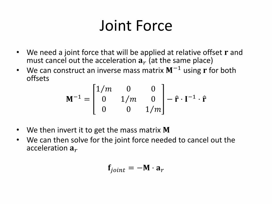
Joint Force
• We need a joint force that will be applied at relative offset 𝐫 and must cancel out the acceleration 𝐚𝑟 (at the same place)
• We can construct an inverse mass matrix 𝐌−1 using 𝐫 for both offsets
𝐌−1 =1 𝑚 0 00 1 𝑚 00 0 1 𝑚
− 𝐫 ⋅ 𝐈−1 ⋅ 𝐫
• We then invert it to get the mass matrix 𝐌 • We can then solve for the joint force needed to cancel out the
acceleration 𝐚𝑟
𝐟𝑗𝑜𝑖𝑛𝑡 = −𝐌 ⋅ 𝐚𝑟
Joint Force
• Once we have the joint force, we apply it to the rigid body just as any other force, thus finishing the summation of the total force and torque
• We can then use the total force and torque to integrate the motion forward
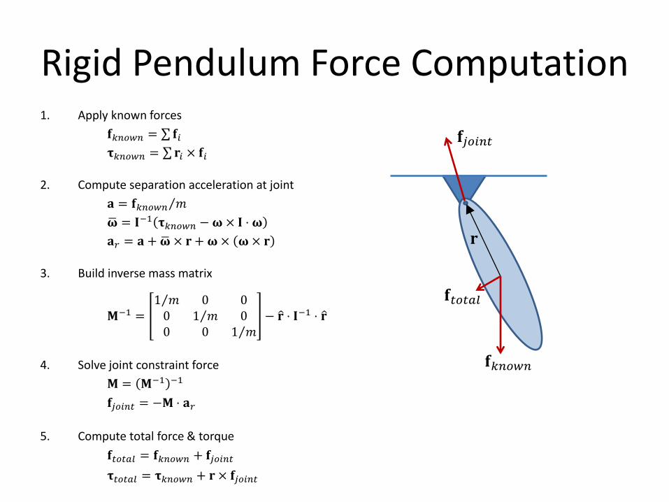
Rigid Pendulum Force Computation 1. Apply known forces
𝐟𝑘𝑛𝑜𝑤𝑛 = 𝐟𝑖
𝛕𝑘𝑛𝑜𝑤𝑛 = 𝐫𝑖 × 𝐟𝑖
2. Compute separation acceleration at joint
𝐚 = 𝐟𝑘𝑛𝑜𝑤𝑛 𝑚
𝛚 = 𝐈−1 𝛕𝑘𝑛𝑜𝑤𝑛 −𝛚× 𝐈 ⋅ 𝛚
𝐚𝑟 = 𝐚 +𝛚 × 𝐫 + 𝛚× 𝛚× 𝐫
3. Build inverse mass matrix
𝐌−1 =1 𝑚 0 00 1 𝑚 00 0 1 𝑚
− 𝐫 ⋅ 𝐈−1 ⋅ 𝐫
4. Solve joint constraint force
𝐌 = 𝐌−1 −1
𝐟𝑗𝑜𝑖𝑛𝑡 = −𝐌 ⋅ 𝐚𝑟
5. Compute total force & torque
𝐟𝑡𝑜𝑡𝑎𝑙 = 𝐟𝑘𝑛𝑜𝑤𝑛 + 𝐟𝑗𝑜𝑖𝑛𝑡
𝛕𝑡𝑜𝑡𝑎𝑙 = 𝛕𝑘𝑛𝑜𝑤𝑛 + 𝐫 × 𝐟𝑗𝑜𝑖𝑛𝑡
𝐫
𝐟𝑘𝑛𝑜𝑤𝑛
𝐟𝑗𝑜𝑖𝑛𝑡
𝐟𝑡𝑜𝑡𝑎𝑙

Joint Error
• Unfortunately, there’s a catch…
• The problem is that the joint forces are changing continuously, and so the finite time integration will accumulate a small error on every step
• An error in the integration of the second derivative means that the first derivative (velocity) and the zeroth derivative (position) will accumulate error
• This error shows up as a non-zero velocity at the joint and as a gap in position as well

Joint Error
• There are several options for correcting the error:
– Penalty forces
– Impulse to correct velocity
– ‘Push’ to correct position
– Construct as kinematic hierarchy
Articulated Bodies

Double Pendulum
• Consider the double pendulum
• Known force 𝐟𝑘1 acts on body 1 and known force 𝐟𝑘2 acts on body 2
• We need to simultaneously solve for joint forces 𝐟𝑗1 and 𝐟𝑗2
that hold both joints together 𝐟𝑘1
𝐟𝑗1
𝐟𝑘2
𝐟𝑗2
−𝐟𝑗2
𝑏𝑜𝑑𝑦 1
𝑏𝑜𝑑𝑦 2
𝑗𝑜𝑖𝑛𝑡 2
𝑗𝑜𝑖𝑛𝑡 1
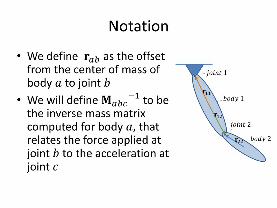
Notation
• We define 𝐫𝑎𝑏 as the offset from the center of mass of body 𝑎 to joint 𝑏
• We will define 𝐌𝑎𝑏𝑐−1 to be
the inverse mass matrix computed for body 𝑎, that relates the force applied at joint 𝑏 to the acceleration at joint 𝑐
𝑏𝑜𝑑𝑦 1
𝑏𝑜𝑑𝑦 2
𝑗𝑜𝑖𝑛𝑡 2
𝑗𝑜𝑖𝑛𝑡 1
𝐫11
𝐫12
𝐫22
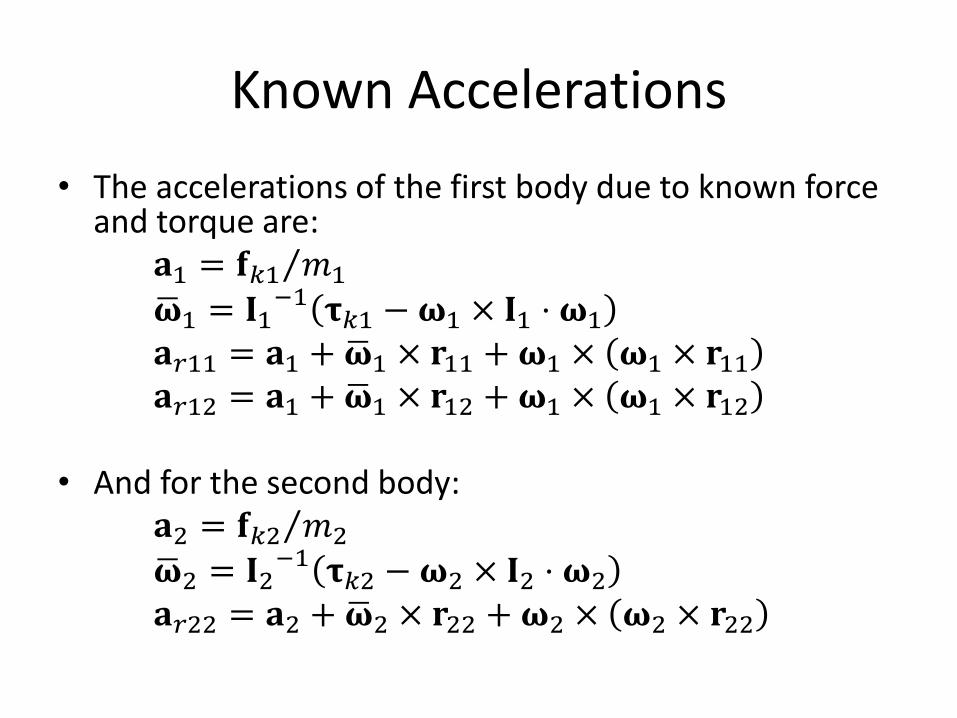
Known Accelerations
• The accelerations of the first body due to known force and torque are:
𝐚1 = 𝐟𝑘1 𝑚1
𝛚 1 = 𝐈1−1 𝛕𝑘1 −𝛚1 × 𝐈1 ⋅ 𝛚1
𝐚𝑟11 = 𝐚1 +𝛚 1 × 𝐫11 +𝛚1 × 𝛚1 × 𝐫11 𝐚𝑟12 = 𝐚1 +𝛚 1 × 𝐫12 +𝛚1 × 𝛚1 × 𝐫12
• And for the second body: 𝐚2 = 𝐟𝑘2 𝑚2
𝛚 2 = 𝐈2−1 𝛕𝑘2 −𝛚2 × 𝐈2 ⋅ 𝛚2
𝐚𝑟22 = 𝐚2 +𝛚 2 × 𝐫22 +𝛚2 × 𝛚2 × 𝐫22
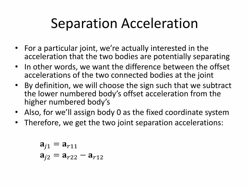
Separation Acceleration
• For a particular joint, we’re actually interested in the acceleration that the two bodies are potentially separating
• In other words, we want the difference between the offset accelerations of the two connected bodies at the joint
• By definition, we will choose the sign such that we subtract the lower numbered body’s offset acceleration from the higher numbered body’s
• Also, for we’ll assign body 0 as the fixed coordinate system • Therefore, we get the two joint separation accelerations:
𝐚𝑗1 = 𝐚𝑟11 𝐚𝑗2 = 𝐚𝑟22 − 𝐚𝑟12

Joint Forces
• The separation acceleration at joint 1 resulting from joint forces will be the sum of accelerations due to 𝐟𝑗1 and −𝐟𝑗2
• The acceleration at joint 1 due to joint forces will be:
𝐚𝑗1′ = 𝐌111
−1 ⋅ 𝐟𝑗1 +𝐌121−1 ⋅ −𝐟𝑗2
𝐚𝑗1′ = 𝐌111
−1 ⋅ 𝐟𝑗1 −𝐌121−1 ⋅ 𝐟𝑗2
• The separation acceleration at joint 2 will be the difference of the accelerations of the offset point on body 2 and the offset point on body 1
𝐚𝑗2′ = 𝐌222
−1 ⋅ 𝐟𝑗2 − 𝐌112−1 ⋅ 𝐟𝑗1 +𝐌122
−1 ⋅ −𝐟𝑗2
𝐚𝑗2′ = −𝐌112
−1 ⋅ 𝐟𝑗1 + 𝐌122−1 +𝐌222
−1 ⋅ 𝐟𝑗2 𝐟𝑘1
𝐟𝑗1
𝐟𝑘2
𝐟𝑗2
−𝐟𝑗2
𝑏𝑜𝑑𝑦 1
𝑏𝑜𝑑𝑦 2
𝑗𝑜𝑖𝑛𝑡 2
𝑗𝑜𝑖𝑛𝑡 1

Joint Forces
𝐚𝑗1′ = 𝐌111
−1 ⋅ 𝐟𝑗1 −𝐌121−1 ⋅ 𝐟𝑗2
𝐚𝑗2′ = −𝐌112
−1 ⋅ 𝐟𝑗1 + 𝐌122−1 +𝐌222
−1 ⋅ 𝐟𝑗2
𝐚𝑗1′
𝐚𝑗2′ =
𝐌111−1 −𝐌121
−1
−𝐌112−1 𝐌122
−1 +𝐌222−1 ⋅
𝐟𝑗1𝐟𝑗2
𝐚𝑗′ = 𝐌−1 ⋅ 𝐟𝑗

Double Pendulum
𝐌−1 =𝐌111
−1 −𝐌121−1
−𝐌112−1 𝐌122
−1 +𝐌222−1
𝐟𝑗 = −𝐌 ⋅ 𝐚𝑗 • To compute the joint forces for the double pendulum:
– Apply known forces – Compute separation acceleration for each joint – Build 6x6 system inverse mass matrix
– Invert mass matrix to solve joint forces with 𝐟𝑗 = −𝐌 ⋅ 𝐚𝑗 – Add joint forces to compute total forces and torques

Articulated Bodies
• We can extend this method to large systems of constrained rigid bodies
• We end up producing a large system mass matrix that relates the vector of all joint forces to the vector of all joint accelerations
• If we assume 𝑛 3-DOF ball joints, we would end up with a 3𝑛 × 3𝑛 mass matrix describing the relationship between joint forces and joint separation accelerations

Constraint Types
• We’ve looked at 3-DOF ball-and-socket joints • These are nice because they require solving a
straightforward 3D force • However, other joint types are also possible such
as 1-DOF hinges, 2-DOF universal joints, 1-DOF translational ‘prismatic’ joints, and more
• These other joint types can apply a constraint force as well as torques
• A 1-DOF hinge joint, for example, applied 5 constraints: 3 forces, and 2 torques, leaving 1 DOF free to rotate
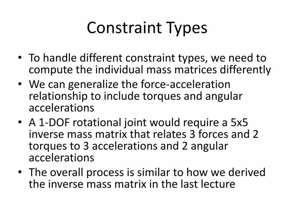
Constraint Types
• To handle different constraint types, we need to compute the individual mass matrices differently
• We can generalize the force-acceleration relationship to include torques and angular accelerations
• A 1-DOF rotational joint would require a 5x5 inverse mass matrix that relates 3 forces and 2 torques to 3 accelerations and 2 angular accelerations
• The overall process is similar to how we derived the inverse mass matrix in the last lecture

System Mass Matrix
• For a system of articulated rigid bodies, we end up with an 𝑚 ×𝑚 mass matrix that relates constraint forces to accelerations, where 𝑚 is the total number of constrained degrees of freedom
• We see that a large system of constraints results in a large matrix that must be inverted
• The matrix will be more sparse for loosely coupled systems and less sparse for tightly coupled systems
• The matrix will also be positive definite • There are several approaches to solving this system:
– Direct matrix solution – Pairwise solution – Recursive solution (Featherstone’s algorithm) – Lagrangian formulation
Direct Solution
• If we have a dense mass matrix, we can directly invert with standard matrix inversion or solvers
• Larger matrices tend to be more sparse, and so can benefit from special purpose sparse solvers
• There are a variety of special purpose solvers that can take advantage of properties of the system (sparseness, positive-definiteness…)
Pairwise Algorithms
• One can also use pairwise algorithms to solve large systems of constraints
• With this method, we group all constraints into a queue, ordered by the magnitude of the separation accelerations
• We then iteratively solve for the constraint at the top of the queue, and then add it to the known forces, recomputing separation accelerations of connected joints and re-ordering the queue as needed
• Basically, this method continues to fix the constraint with the largest separation and repeats until it converges and all separations approach zero
Featherstone’s Algorithm
• Featherstone’s algorithm is a recursive method for solving the dynamics of tree structures without kinematic loops
• It can evaluate systems in linear O(n) time • It traverses from the fixed base (or an unfixed root) to the
leaf nodes computing joint separation accelerations and accumulating a mass matrix connecting from the base to each leaf
• Then, it solves the joint forces from the leaves progressing back to the root
• There are some adaptations to handle kinematic loops, but they compromise the linear time behavior
• “Robot Dynamics Algorithms”, Featherstone, 1987
Lagrangian Dynamics
• We can also reformulate the equations into the Lagrangian form • This is fairly different from how we’ve done things so far • Lagrangian methods define the state of the system using
generalized coordinates, only using coordinates for actual DOFs in the system
• In this approach, the constraints never actually need to be solved, but we do have to solve for the motion of the degrees of freedom
• If the number of unconstrained DOFs is less than the number of constrained DOFs, then these methods can be faster than the Newtonian methods described so far
• However, the method can be tricky to work with and doesn’t handle collisions or energy damping easily

Kinematic Loops
• We often distinguish between articulated bodies with open tree-like structures from bodies with closed kinematic loops
• Closed loops can add challenges to some of the solution methods, as they may result in over-constrained systems and non-invertible mass matrices
• Some methods require special handling for these, while other methods (like pairwise solvers) don’t require anything special

Collisions
Detection and Response
• Collision handling requires two different technologies: – Collision detection (geometry) – Collision response (physics)
• The collision detection problem is a complex application of 3D geometry and spatial data structures, and will be discussed in more detail in the next lecture
• Collision response is the physics problem of determining the forces (or impulses) resulting from the collisions
Impact vs. Contact
• It is useful to distinguish between momentary (instantaneous) impacts and finite time contacts
• With impacts, the closing velocity is positive before the collision, and with contacts, the closing velocity is zero (or very close)
• Some rigid body methods handle impacts differently from contacts, while other methods don’t distinguish between the two
Impulse
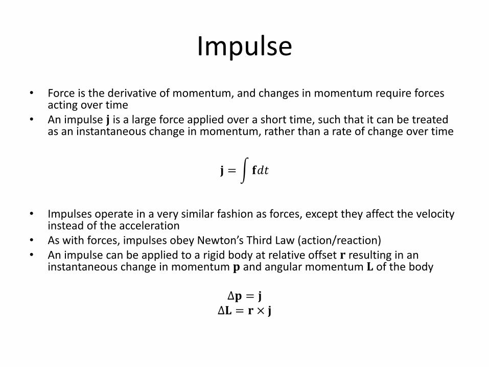
• Force is the derivative of momentum, and changes in momentum require forces acting over time
• An impulse 𝐣 is a large force applied over a short time, such that it can be treated as an instantaneous change in momentum, rather than a rate of change over time
𝐣 = 𝐟𝑑𝑡
• Impulses operate in a very similar fashion as forces, except they affect the velocity
instead of the acceleration • As with forces, impulses obey Newton’s Third Law (action/reaction) • An impulse can be applied to a rigid body at relative offset 𝐫 resulting in an
instantaneous change in momentum 𝐩 and angular momentum 𝐋 of the body
∆𝐩 = 𝐣 ∆𝐋 = 𝐫 × 𝐣

Collision Impulses
• Most rigid body methods resolve instantaneous impacts with impulses
• Persistent contacts can be simulated with forces or impulses, but many modern methods use impulses
• In fact, constraints can be handled through forces or impulses as well, and by using impulses, one can handle impacts, contacts, and constraints through a single process
Single Body Impact
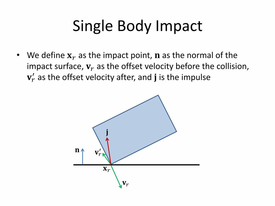
• We define 𝐱𝑟 as the impact point, 𝐧 as the normal of the impact surface, 𝐯𝑟 as the offset velocity before the collision, 𝐯𝑟′ as the offset velocity after, and 𝐣 is the impulse
𝐯𝑟
𝐯𝑟′ 𝐧
𝐱𝑟
𝐣

Collision Restitution
• In terms of collisions, restitution refers to the amount of kinetic energy that is conserved, and thus the amount of bounce
• We can measure it with a coefficient of restitution 𝜀 that will range from 0 (perfectly inelastic) to 1 (perfectly elastic)
• For simplicity, we can assume that we have a constant restitution for a rigid body. If two rigid bodies of different restitution collide, it is a reasonable heuristic to use the lower of the two for the impulse computation
• Note: there are different ways to define the exact meaning of this constant, and it is ultimately just an approximation to a far more complex process that is dependent on the material properties and shape of the object
• Note: sometimes called coefficient of elasticity

Collision Impulse
• We need a collision impulse that will be applied at relative offset 𝐫 and must cancel out the velocity 𝐯𝑟 (at the same place)
• We can construct an inverse mass matrix 𝐌−1 using 𝐫 for both offsets
𝐌−1 =1 𝑚 0 00 1 𝑚 00 0 1 𝑚
− 𝐫 ⋅ 𝐈−1 ⋅ 𝐫
• We then invert it to get the mass matrix 𝐌 • We can then solve for the impulse needed to cancel out the velocity
𝐯𝑟
𝐣𝑖𝑚𝑝𝑎𝑐𝑡 = − 1 + 𝜀 𝐌 ⋅ 𝐯𝑟

*Frictionless Impact
• [insert slide here]

Friction
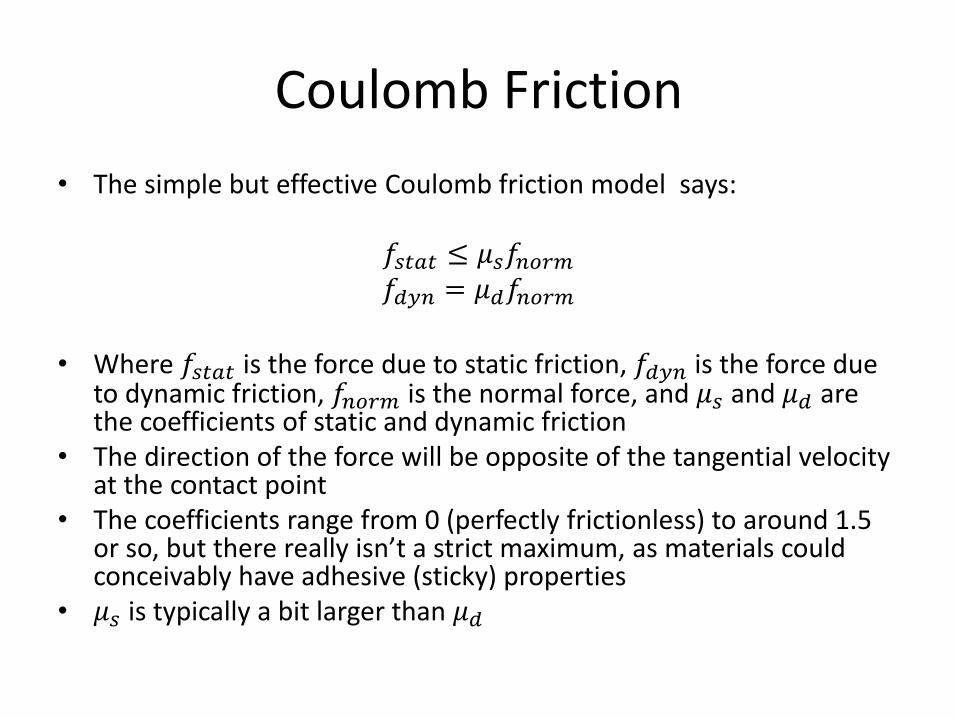
Coulomb Friction
• The simple but effective Coulomb friction model says:
𝑓𝑠𝑡𝑎𝑡 ≤ 𝜇𝑠𝑓𝑛𝑜𝑟𝑚 𝑓𝑑𝑦𝑛 = 𝜇𝑑𝑓𝑛𝑜𝑟𝑚
• Where 𝑓𝑠𝑡𝑎𝑡 is the force due to static friction, 𝑓𝑑𝑦𝑛 is the force due to dynamic friction, 𝑓𝑛𝑜𝑟𝑚 is the normal force, and 𝜇𝑠 and 𝜇𝑑 are the coefficients of static and dynamic friction
• The direction of the force will be opposite of the tangential velocity at the contact point
• The coefficients range from 0 (perfectly frictionless) to around 1.5 or so, but there really isn’t a strict maximum, as materials could conceivably have adhesive (sticky) properties
• 𝜇𝑠 is typically a bit larger than 𝜇𝑑

Friction Cone
• Consider a block sliding on a flat surface
• The ground applies a normal force and a friction force
• According to the Coulomb friction model, the two forces must add up to a vector that lies within the friction cone
• The same can be said about impulses resulting from impacts
𝐣
𝜇
1
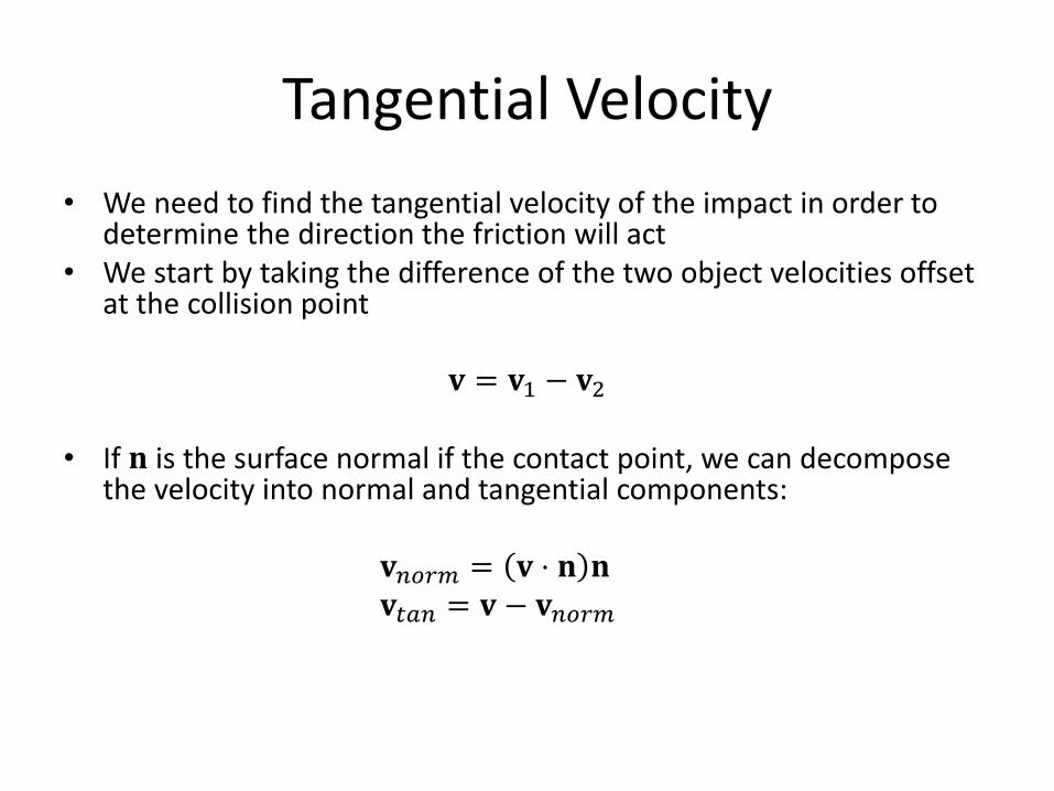
Tangential Velocity
• We need to find the tangential velocity of the impact in order to determine the direction the friction will act
• We start by taking the difference of the two object velocities offset at the collision point
𝐯 = 𝐯1 − 𝐯2 • If 𝐧 is the surface normal if the contact point, we can decompose
the velocity into normal and tangential components:
𝐯𝑛𝑜𝑟𝑚 = 𝐯 ⋅ 𝐧 𝐧 𝐯𝑡𝑎𝑛 = 𝐯 − 𝐯𝑛𝑜𝑟𝑚

Rolling & Spinning Friction
• One can also add rolling and spinning friction effects to collisions and contacts
• We must first find the angular velocity difference at the collision point • From there, we can decompose it into rolling and spinning components
based on the contact normal 𝐧
𝛚𝑠𝑝𝑖𝑛 = 𝛚 ⋅ 𝐧 𝐧
𝛚𝑟𝑜𝑙𝑙 = 𝛚−𝛚𝑠𝑝𝑖𝑛 • We can then apply friction torques proportional to each of those based on
separate constants
𝛕𝑓𝑟𝑖𝑐 = − 𝐟𝑛𝑜𝑟𝑚 𝜇𝑠𝑝𝑖𝑛𝛚𝑠𝑝𝑖𝑛 + 𝜇𝑟𝑜𝑙𝑙𝛚𝑟𝑜𝑙𝑙
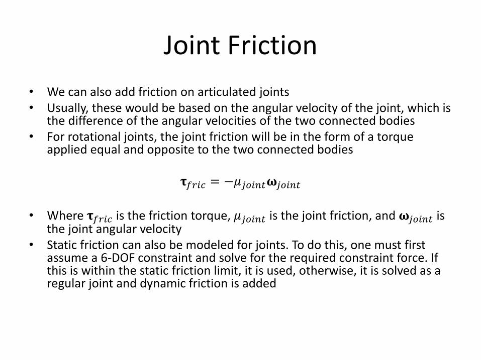
Joint Friction
• We can also add friction on articulated joints • Usually, these would be based on the angular velocity of the joint, which is
the difference of the angular velocities of the two connected bodies • For rotational joints, the joint friction will be in the form of a torque
applied equal and opposite to the two connected bodies
𝛕𝑓𝑟𝑖𝑐 = −𝜇𝑗𝑜𝑖𝑛𝑡𝛚𝑗𝑜𝑖𝑛𝑡
• Where 𝛕𝑓𝑟𝑖𝑐 is the friction torque, 𝜇𝑗𝑜𝑖𝑛𝑡 is the joint friction, and 𝛚𝑗𝑜𝑖𝑛𝑡 is the joint angular velocity
• Static friction can also be modeled for joints. To do this, one must first assume a 6-DOF constraint and solve for the required constraint force. If this is within the static friction limit, it is used, otherwise, it is solved as a regular joint and dynamic friction is added

Collision Impulse with Friction
• We wish to find a collision impulse 𝐣 that accounts for the elasticity and friction • We can compute the velocity of the colliding point at offset 𝐫 as:
𝐯𝑟 = 𝐯 + 𝛚 × 𝐫
𝐯𝑛𝑜𝑟𝑚 = 𝐯𝑟 ⋅ 𝐧 𝐧 𝐯𝑡𝑎𝑛 = 𝐯𝑟 − 𝐯𝑛𝑜𝑟𝑚
• We also build the inverse mass matrix 𝐌−1 for the body using 𝐫 for both offsets • We start by assuming perfect static friction and solving for the impulse that would result in an
elastic bounce and the tangential velocity going to zero after the collision:
𝐯𝑛𝑜𝑟𝑚′ = −𝜀𝐯𝑛𝑜𝑟𝑚
𝐣0 = 𝐌 ⋅ 𝐯𝑛𝑜𝑟𝑚′ − 𝐯𝑛𝑜𝑟𝑚
• This allows us to solve the impulse that produces this result • If this lies within the friction cone, then we’re done • Otherwise, we assume sliding (dynamic) friction • For more details, see section 7 of “Nonconvex Rigid Bodies with Stacking”, Guendelman, Bridson,
Fedkiw, 2003

Multibody Collisions
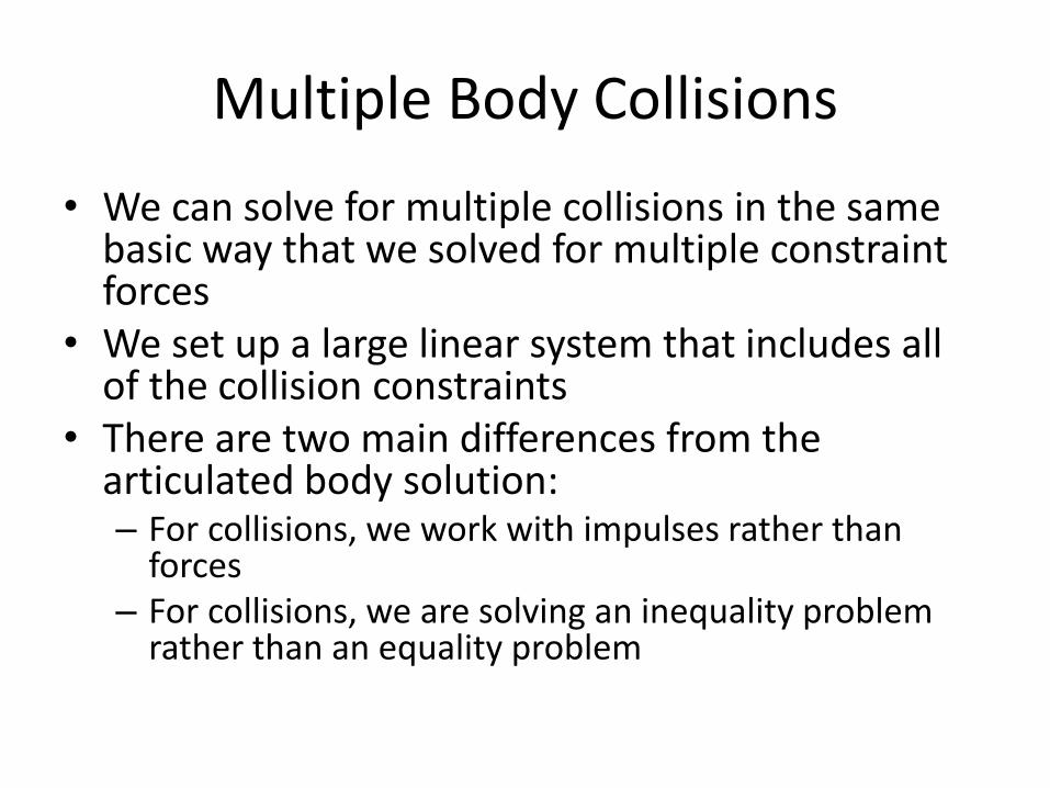
Multiple Body Collisions
• We can solve for multiple collisions in the same basic way that we solved for multiple constraint forces
• We set up a large linear system that includes all of the collision constraints
• There are two main differences from the articulated body solution: – For collisions, we work with impulses rather than
forces – For collisions, we are solving an inequality problem
rather than an equality problem

Linear Complementarity
• Collisions result in inequality constraints because they will only act to prevent objects from moving towards each other and have no effect on objects moving apart
• A large system of inequalities can be formed into a linear complementarity problem (LCP) which is a well studied class of problems
• Various solution methods have been proposed to address these, and some are discussed in the overview paper on the web page
Pairwise Solvers
• Pairwise solvers iteratively solve one collision at a time until the entire system is satisfied
• These have proven to be pretty effective in handling of multiple collisions and constraints, as each one can be treated with its own rules and special cases
• Some other methods may be faster, but pairwise solvers tend to be very general purpose and easy to implement