CONSTRUCTING COMMON FACTORS FROM CONTINUOUS ANDCATEGORICAL DATA

Serena Ng

Department of EconomicsColumbia University∗

December 2012

Abstract

The method of principal components is widely used to estimate common factors in largepanels of continuous data. This paper first reviews alternative methods that obtain the commonfactors by solving a Procrustes problem. While these matrix decomposition methods do notspecify the probabilistic structure of the data and hence do not permit statistical evaluations ofthe estimates, they can be extended to analyze categorical data. This involves the additionalstep of quantifying the ordinal and nominal variables. The paper then reviews and explores thenumerical properties of these methods. An interesting finding is that the factor space can bequite precisely estimated directly from categorical data without quantification. This may requireusing a larger number of estimated factors to compensate for the information loss in categoricalvariables. Separate treatment of categorical and continuous variables may not be necessary ifstructural interpretation of the factors is not required, such as in forecasting exercises.

Keywords: factor models, principal components, ordinal data, alternating least squares.

JEL Classification: C5, C6, C25, C35

∗Correspondence: 420 W. 118 St. New York, NY 10025. Email: serena.ng@columbia.eduI thank Aman Ullah for teaching me econometrics and especially grateful for his guidance and support over theyears. Comments from two anonymous referees are greatly appreciated. I also thank Nickolay Trendafilov for helpfulcomments and discussions. Financial support from the National Science Foundation (SES-0962431) is gratefullyacknowledged.

1 Introduction

The recent interest of economists in factor models is largely driven by the fact that common

factors estimated from large panels of data often have predictive power for economic variables of

interest. Theoretical and empirical work predominantly use principal components to estimate the

common factors in continuous data. Little attention has been given to alternative estimators and

to the treatment of categorical data even though many economic variables are of this nature. For

example, households and firms are asked in surveys whether they expect economic conditions to

improve or not. While such data could be useful for forecasting, they cannot be approximated by

continuous distributions. This paper first reviews dimension reduction methods that can handle

mixed measurement data, meaning that the data can be continuous or categorical. I then investigate

the consequence from the perspective of the factor space of using categorical variables to construct

principal components, treating the data as if they were continuous.

Any study of socio-economic status necessarily involves analyzing dichotomous data or data

with a small number of categories. Such data requires special treatment as they contain important

but imperfect information about the underlying latent variables. Racine and Li (2004) and Su

and Ullah (2009) consider using a small set of mixed data in non-parametric regressions. Here, I

consider the situation when the set of mixed predictors is large enough that dimenional reduction

becomes necessary. As pointed out in Kolenikov and Angeles (2009) and further investigated below,

the method that is currently used by economists is far from satisfactory.

The psychometric approach to the dimension reduction problem is to either explicitly model

the latent continuous variables or quantify (impute) the continuous variables from the categorical

data.1 According to the SPSS software and as explained in Meulman and Heiser (2001), three types

of categorical variables are relevant: - (1) nominal variables which represent unordered categories

(such as zip codes and SIC codes); (2) ordinal variables which represent ordered categories (such

as satisfaction ratings of excellent/good/average/poor and Likert scale), and (3) numerical (count)

variables which represent ordered categories (such as age in years and income class in dollars) with

distances between categories that can be meaningfully interpreted. Nominal and ordinal data are

said to be non-metrical because the distance between two categories has no meaningful interpreta-

tion. The challenge for factor analysis of non-metrical data lies in the fact that normalization and

monotonicity constraints need to be imposed to ensure consistency between the imputed variables

and the observed discrete variables. Not surprisingly, going down this route necessarily takes us

from linear to non-linear methods of dimension reduction.

I begin with a review of factor analysis of continuous data from the viewpoint of solving a

1An 1983 issue of Journal of Econometrics, (de Leeuw and Wansbeek editors) was devoted to these methods.

1

Procrustes problem. These methods are non-probabilistic and do not permit formal inference to be

made. But they form the basis of many dimension reduction problems which are interesting in their

own right. The issues that arise in factor analysis of categorical data are then discussed. Special

focus is given to methods that quantify the discrete data. Simulations are used to evaluate the

precision of the factors estimated from continuous and mixed data. The so-called Filmer Pritchett

procedure is also evaluated. I assess the factors estimates from the perspective of diffusion index

forecasting which requires extracting common information in a large number of categorical variables.

Precise estimation of the factor space rather than structural interpretation of the factor estimates

takes center-stage.2 An interesting finding is that the principal components of the raw discrete

data can estimate the factor space reasonably precisely, though this may require over-estimating

the number of factors to compensate for the information loss in categorical data. Data quantification

may not be necessary.

2 Factor Analysis of Continuous Data

Factor analysis is a statistical framework used to analyze the behavior of observed variables using

a small number of unobserved factors. Spearman (1904) appears to be the first to conjecture

that a common unobserved trait (mental ability) may be responsible for the positive correlation in

children’s test scores on a variety of subjects. To analyze the contribution of the factors on the test

scores and more generally on data that are continuous, the classical approach is to estimate the

factor loadings by maximizing the Gaussian likelihood. Important contributions have subsequently

been made by Anderson and Rubin (1956), Joreskog (1970), Lawley and Maxwell (1971), and

Browne (1984), among others. Factor models are now used not just by psychologists, but by

researchers in marketing, biology, and other fields.

Let X denote a T ×N matrix of continuous data or data in ratio form. As a matter of notation,

the i, j entry of X is denoted Xij ; Xi,: is the i-th row of X and X:,j is the j-th column. For

macroeconomic panels, N is the number of variables and T is the number of time periods over

which the variables are observed. A superscript zero is used to denote true values. The goal of

factor analysis is to explain X using r common factors F 0 = (F 01 , . . . , F

0r ) and N idiosyncratic

errors e0. In matrix form, the factor representation of the data is

X = F 0Λ0′ + e0.

where Λ0 is a N × r matrix of factor loadings. The population covariance structure of X under the

2The focus is rather different from the structural factor analysis considered in Cunha and Heckman (2008); Almund,Duckworth, Heckman, and Kautz (2011).

2

assumption that the factors have unit variance and are mutually uncorrelated is

Σ0X = Λ0Λ0′ + Ω0.

In classical factor analysis, Ω0 is assumed to be a diagonal matrix and the data X are said to

have a strict factor structure. Let k be the assumed number of factors which can be different

from r. Anderson and Rubin (1956) assume that the data are multivariate normal. They use

the normalization ΣF 0 = Ir and suggest to estimate the factor loadings by maximizing the log

likelihood:

log L0(Λ,Ω; k) = log |Ω|+ trace (X − FΛ′)Ω−1(X − FΛ′)′.

Lawley and Maxwell (1971) consider the equivalent problem of maximizing

logL1(Λ,Ω; k) = log |ΣX |+ trace (SXΣ−1X )− log |SX | −N

where SX is the sample covariance of X. An advantage of maximum likelihood estimation is that

the sampling distribution of Λ is known and inference can be made. When T is large and N is

fixed, the factor estimates Λ are√T consistent and asymptotically normal. Unbiased estimates of

F can be obtained as shown in Lawley and Maxwell (1971, Ch.8) even though these are not usually

the object of interest in psychology research.

When the normality assumption is not appropriate, one alternative is to consider covariance

structure estimation (also known as structural equation modeling). Let θ = (vec (Λ), vech (Ω))′

be the parameters of the factor model and W be a weighting matrix. The weighted least squares

estimator is

θWLS = argminθ

(vech (ΣX(θ)− vech (SX))′W (vech (ΣX(θ)− vech (SX)).

Under regularity conditions and assuming that N is fixed, the WLS estimator is also√T consistent

and asymptotically normal, as shown in Browne (1984) and others. As θWLS is simply a method

of moments estimator, it is less efficient than MLE but is robust to departures from normality.

Assuming that the true number of factors is known, it has been documented that the asymptotic

approximation of the WLS estimator is not accurate when the data exhibit excess kurtosis; the

chi-square statistic for goodness of fit is oversized; the factor loadings are underestimated, and the

standard error of the estimates tend to be downward biased.

Another alternative to MLE is iterative least squares estimation, the best known in this category

being MINRES. Given a N × N sample correlation matrix RX , the objective is to find a N × Nmatrix Ω and a N × k matrix Λ such that ΛΛ′ is as close to RX as possible. Formally,

LMINRES(Λ; k) =∥∥RX − ΛΛ′ − Ω

∥∥2 .3

Concentrating out Ω and using the fact that the diagonal entries of RX all equal one, the concen-

trated loss function is

LcMINRES(Λ; k) =∑i 6=j

(RX,ij − Λi,:Λ′j,:)

2

where Λi,: is the i-th row of Λ, and RX,ij is the (i, j) entry of RX . Harman and Jones (1966) suggest

to start with an arbitrary Λ and iterate on each row of Λ holding other rows fixed. To update the

rows, the objective function is separated into a part that depends on Λi,: and a part ci that does

not. Let R−iX be the i-th column of RX with the i-element excluded, and let Λ−i be the (N −1)×kmatrix of Λ when the i-th row is deleted. Define

LcMRS,i(Λi,:; k) = (RX,1i − Λ1,:Λ′i,:)

2 + (RX,i−1,i − Λi−1,:Λ′i,:)

2 +

(RX,i+1,i − Λi+1,:Λ′i,:)

2 + . . .+ (RX,ki − Λk,:Λ′i,:)

2 + ci

=∥∥R−iX − Λ−iΛ′i,:

∥∥2 + ci

The solution to this minimization problem is standard; it is the least squares estimate

Λ′i,: = (Λ−i′Λ−i)−1Λ−i

′R−iX .

Since all units other than i are held fixed when Λi,: is constructed, the estimator is based on the

principle of alternating least squares. Iterative updating of the i-th row of Λ has been shown to

decrease the loss function. However, a researcher would not be able to say whether a poor fit is

due to the idiosyncratic errors or omitted factors. One shortcoming of MINRES is that Λi,:Λ′i,:

can exceed one, which would then imply a negative idiosyncratic error variance. This so-called

Heywood case can be circumvented. An example is the LISREL implementation of MINRES,

detailed in Joreskog (2003).

Strict (or exact) factor models are to be contrasted with models more widely used in macroe-

conomics and finance. These models relax the assumption of strict factor models to allow some

cross-section and serial correlation in eit. Chamberlain and Rothschild (1983) referred to these as

approximate factor models. Estimation is based on the method of asymptotic principal components

(PCA) first proposed in Connor and Korajzcyk (1986). The estimator minimizes

LPCA(Λ, F ; k) =1

NT

N∑i=1

T∑t=1

(xit − Λi,:Ft)2 =

1

NT

N∑i=1

(X:,i − FΛ′i)′(X:,i − FΛ′i).

Because Λ′i,: = (F ′F )−1F ′X:.i for any given F , the concentrated objective function is:

LcPCA(F ; Λ; k) =1

NT

N∑i=1

(X:,i − PFX:,i)′(X:,i − PFX:,i)

=1

NT

N∑i=1

X ′:,iX:,i −1

N

N∑i=1

X ′:,iPFX:,i

4

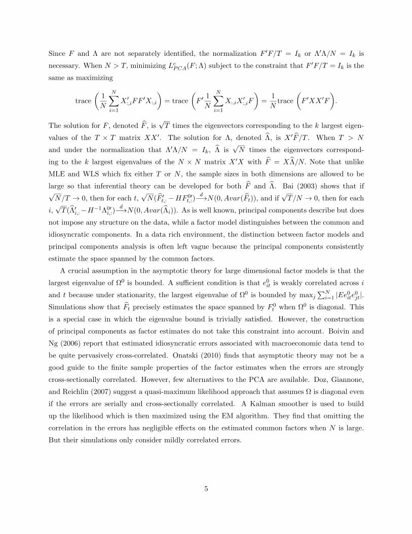
Since F and Λ are not separately identified, the normalization F ′F/T = Ik or Λ′Λ/N = Ik is

necessary. When N > T, minimizing LcPCA(F ; Λ) subject to the constraint that F ′F/T = Ik is the

same as maximizing

trace

(1

N

N∑i=1

X ′:,iFF′X:,i

)= trace

(F ′

1

N

N∑i=1

X:,iX′:,iF

)=

1

Ntrace

(F ′XX ′F

).

The solution for F , denoted F , is√T times the eigenvectors corresponding to the k largest eigen-

values of the T × T matrix XX ′. The solution for Λ, denoted Λ, is X ′F /T . When T > N

and under the normalization that Λ′Λ/N = Ik, Λ is√N times the eigenvectors correspond-

ing to the k largest eigenvalues of the N × N matrix X ′X with F = XΛ/N. Note that unlike

MLE and WLS which fix either T or N , the sample sizes in both dimensions are allowed to be

large so that inferential theory can be developed for both F and Λ. Bai (2003) shows that if√N/T → 0, then for each t,

√N(F ′t,:−HF 0′

t,:)d−→N(0, Avar(Ft)), and if

√T/N → 0, then for each

i,√T (Λ′i,:−H−1Λ0′

i,:)d−→N(0, Avar(Λi)). As is well known, principal components describe but does

not impose any structure on the data, while a factor model distinguishes between the common and

idiosyncratic components. In a data rich environment, the distinction between factor models and

principal components analysis is often left vague because the principal components consistently

estimate the space spanned by the common factors.

A crucial assumption in the asymptotic theory for large dimensional factor models is that the

largest eigenvalue of Ω0 is bounded. A sufficient condition is that e0it is weakly correlated across i

and t because under stationarity, the largest eigenvalue of Ω0 is bounded by maxj∑N

i=1 |Ee0ite0jt|.Simulations show that Ft precisely estimates the space spanned by F 0

t when Ω0 is diagonal. This

is a special case in which the eigenvalue bound is trivially satisfied. However, the construction

of principal components as factor estimates do not take this constraint into account. Boivin and

Ng (2006) report that estimated idiosyncratic errors associated with macroeconomic data tend to

be quite pervasively cross-correlated. Onatski (2010) finds that asymptotic theory may not be a

good guide to the finite sample properties of the factor estimates when the errors are strongly

cross-sectionally correlated. However, few alternatives to the PCA are available. Doz, Giannone,

and Reichlin (2007) suggest a quasi-maximum likelihood approach that assumes Ω is diagonal even

if the errors are serially and cross-sectionally correlated. A Kalman smoother is used to build

up the likelihood which is then maximized using the EM algorithm. They find that omitting the

correlation in the errors has negligible effects on the estimated common factors when N is large.

But their simulations only consider mildly correlated errors.

5

3 Two Alternating Least Squares Estimators (ALS)

As alternatives to the method of principal components, I consider two estimators (ALS1 and ALS2)

that address the Haywood problem of negative idiosyncratic error variances. ALS2 additionally

allows us to assess if the common and idiosyncratic components are poorly estimated. As distinct

from all estimators considered in the previous section, the idiosyncratic errors are also objects of

interest, putting them on equal footing with the common factors. Furthermore, the factors are

estimated without writing down the probability structure of the model and as such, the statistical

properties of the estimates are not known. It may perhaps be inappropriate to call these estimators.

My interest in these methods arises because they can be extended to study latent variable models

for mixed (discrete and continuous) data.

Whereas the standard approach to deriving an estimator is to take derivatives of the objective

function, a derivative free alternative is to exploit information in the objective function evaluated

at the upper or lower bound. For example, consider finding the minimum of f(x) = x2 − 6x+ 11.

By completing the squares and writing f(x) = (x − 3)2 + 2, it is clear that the lower bound for

f(x) is 2 and is achieved at x = 3. Knowing the lower bound helps to determine the minimizer.3

ten Berge (1993) and Kiers (2002) provide a formal treatment of using bounds to solve matrix

optimizaiton problems.

Lemma 1 Let Y be of order p × q with singular value decomposition Y = PDQ′. Let di be the

i-th diagonal value of D. Then (i) trace (B′Y ) ≤∑q

i=1 di ; and (ii) The maximum of trace (B′Y )

subject to the constraint B′B = I is achieved by setting B = PQ′.

Kristof’s upper bound for trace functions states that if G is a full rank orthonormal matrix

and D is diagonal, then the upper bound of trace (GD) is∑n

i=1 di. ten Berge (1993) generalizes

the argument to sub-orthonormal matrices of rank r ≤ n. Now trace (B′Y ) = trace (B′PDQ′) =

trace (Q′B′PD).4 Part (i) follows by letting G = Q′B′P . Part (ii) says that the upper bound under

the orthogonality constraint is attained by setting G = I or equivalently, B = PQ′. This second

result is actually the solution to the orthogonal ‘Procrustes problem’ underlying many dimension

reduction problems and is worthy of a closer look.5

Let A be a n ×m matrix (of rank r ≤ m ≤ n) and let C be a n × k matrix with a specified

structure. The orthogonal Procrustes problem looks for an orthogonal matrix B of dimension

3It is important that the lower bound is attainable and does not depend on x. If the lower bound was 1 insteadof 2, no meaning could be attached to x = 3 because the lower bound of 1 is not attainable.

4A matrix is sub-orthonormal if it can be made orthonormal by appending rows or columns.5The orthogonal Procrustes problem was solved in Schonmenn (1966). See Gower and Dijksterhuis (2004) for a

review for subsequent work.

6

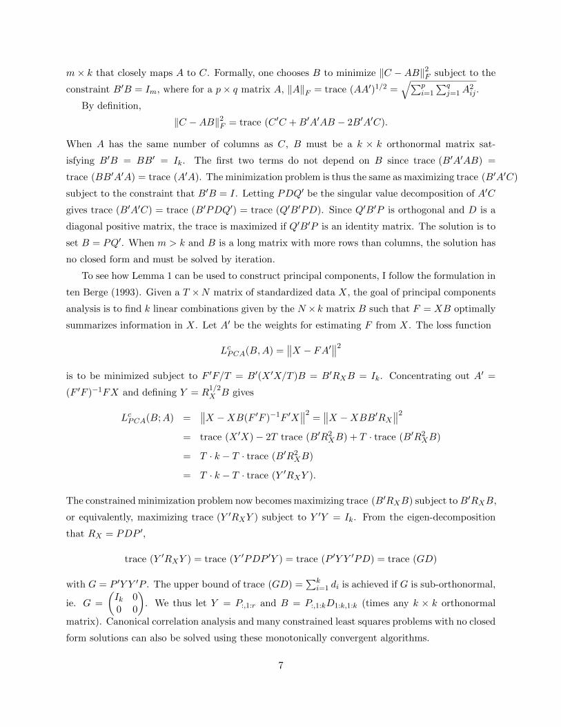
m× k that closely maps A to C. Formally, one chooses B to minimize ‖C −AB‖2F subject to the

constraint B′B = Im, where for a p× q matrix A, ‖A‖F = trace (AA′)1/2 =√∑p

i=1

∑qj=1A

2ij .

By definition,

‖C −AB‖2F = trace (C ′C +B′A′AB − 2B′A′C).

When A has the same number of columns as C, B must be a k × k orthonormal matrix sat-

isfying B′B = BB′ = Ik. The first two terms do not depend on B since trace (B′A′AB) =

trace (BB′A′A) = trace (A′A). The minimization problem is thus the same as maximizing trace (B′A′C)

subject to the constraint that B′B = I. Letting PDQ′ be the singular value decomposition of A′C

gives trace (B′A′C) = trace (B′PDQ′) = trace (Q′B′PD). Since Q′B′P is orthogonal and D is a

diagonal positive matrix, the trace is maximized if Q′B′P is an identity matrix. The solution is to

set B = PQ′. When m > k and B is a long matrix with more rows than columns, the solution has

no closed form and must be solved by iteration.

To see how Lemma 1 can be used to construct principal components, I follow the formulation in

ten Berge (1993). Given a T ×N matrix of standardized data X, the goal of principal components

analysis is to find k linear combinations given by the N ×k matrix B such that F = XB optimally

summarizes information in X. Let A′ be the weights for estimating F from X. The loss function

LcPCA(B,A) =∥∥X − FA′∥∥2

is to be minimized subject to F ′F/T = B′(X ′X/T )B = B′RXB = Ik. Concentrating out A′ =

(F ′F )−1FX and defining Y = R1/2X B gives

LcPCA(B;A) =∥∥X −XB(F ′F )−1F ′X

∥∥2 =∥∥X −XBB′RX∥∥2

= trace (X ′X)− 2T trace (B′R2XB) + T · trace (B′R2

XB)

= T · k − T · trace (B′R2XB)

= T · k − T · trace (Y ′RXY ).

The constrained minimization problem now becomes maximizing trace (B′RXB) subject toB′RXB,

or equivalently, maximizing trace (Y ′RXY ) subject to Y ′Y = Ik. From the eigen-decomposition

that RX = PDP ′,

trace (Y ′RXY ) = trace (Y ′PDP ′Y ) = trace (P ′Y Y ′PD) = trace (GD)

with G = P ′Y Y ′P . The upper bound of trace (GD) =∑k

i=1 di is achieved if G is sub-orthonormal,

ie. G =

(Ik 00 0

). We thus let Y = P:,1:r and B = P:,1:kD1:k,1:k (times any k × k orthonormal

matrix). Canonical correlation analysis and many constrained least squares problems with no closed

form solutions can also be solved using these monotonically convergent algorithms.

7

3.1 ALS1

I first consider the estimator proposed in De Leeuw (2004), Unkel and Trendafilov (2010) and

Trendafilov and Unkel (2011). Let e = uΨ where u′u = IN . Let k be the number of assumed (not

necessarily equal r, the true) number of factors. Suppose first that T ≥ N and consider maximizing

LALS1(F,Λ, u,Ψ; k) =∥∥X − FΛ′ − uΨ

∥∥2F

subject to (i) F ′F = Ik, (ii) u′u = IN , (iii) u′F = 0N×k, (iv) Ψ is diagonal.

Notice that ALS minimizes the difference between the X and its fitted value X = F Λ′+e. While

the idiosyncratic and the common components are explicitly chosen, distributional assumptions on

e are not made. Furthermore, the objective function takes into account the off-diagonal entries of

the fitted correlations. In contrast, the PCA loss function only considers the diagonal entries of

(X − FΛ)′(X − FΛ′). Define

BT×(k+N)

=(F U

), A

N×(k+N)

=(Λ Ψ

).

The ALS estimates are obtained by minimizing

LALS1(B,A; k) =∥∥X −BA′∥∥2

Fsubject to B′B = IN+k.

But for given A, this is the same as maximizing trace (B′XA) over B satisfying B′B = IN+k. The

problem is now in the setup of Lemma 1. When N ≤ T , the estimates (F , Λ, U) can be obtained

using the following three step procedure:

1 Let B = PQ′ where svd(XA) = PDQ′.

2 From B =(B:,1:k|B:,k+1:k+N

), let F = B:,1:k and U = B:,k+1:N . Update Λ as X ′F .

3 Let Ψ = diag(U ′X).

Steps (1) and (2) are based on part (ii) of Lemma 1. Step (3) ensures that Ψ is diagonal and is

motivated by the fact that

U ′X = U ′FΛ′ + U ′UΨ.

Steps (1)-(3) are repeated until the objective function does not change. As FΛ′ is observationally

equivalent to FC−1CΛ′ for any orthogonal matrix C, Step (2) can be modified to make the top

k × k sub-matrix of Λ lower triangular. This identification restriction does not affect the fact that

rank (Λ) = min(rank (X), rank (F )) = k.

When N > T , the rank of U ′U is at most T and the constraint U ′U = IN cannot be satisfied.

However, recall that ΣX = ΛΛ′+ΨU ′UΨ. Trendafilov and Unkel (2011) observe that the population

8

covariance structure of the factor model can still be preserved if the constraint ΨU ′U = Ψ holds,

and in that case, Ω = Ψ2 is positive semi-definite by construction. Furthermore, the constraints

F ′F = Ik and U ′F = 0N×k are equivalent to FF ′ + UU ′ = IT and rank (F ) = k. Minimizing

LALS1(B,A; k) =∥∥X −BA′∥∥2

Fsubject to BB′ = IT

is the same as maximizing trace (BA′X ′) which is again a Procrustes problem. The three step

solution given above remains valid when N > T , but the singular value decomposition in step (a)

needs to be applied to A′X ′.

Trendafilov and Unkel (2011) show that the objective function will decreases at each step

and the algorithm will converge from any starting value. However, convergence of the objective

function does not ensure convergence of the parameters. Furthermore B is not unique because it is

given by the singular value decomposition of a rank deficient matrix. In particular, rank (XA) ≤min(rank (X), rank (A)) < rank (X) + k.

3.2 ALS2

To motivate the second estimator, partition F 0 as F 0 =(F 01 F 02

)where F 01 has k columns and

F 02 has r − k columns for some k < r. The data generating process can be written as

X = F 01Λ1′ + F 02Λ2′ + e0 = F 01′Λ1 + e∗.

If k < r factors are assumed, the omitted factors F 02 will be amalgamated with e0 into e∗. Even

though Ω0 is diagonal in the population, the off-diagonal entries of the covariance matrix for e∗

could be non-zero. Without explicitly imposing the restriction that X and e0 are orthogonal, an

estimator may confound e0 with F 02 . Socan (2003) re-examined an (unpublished) idea by H. Kiers

to minimize

LALS2(F,Λ, e; k) =∥∥X − FΛ′ − e

∥∥2F

subject to (i) e′F = 0 (ii) e′e diagonal (iii) e′X diagonal.

As with ALS1, estimation of e is explicitly taken into account. The first two constraints are

standard; the third constraint ensures that the idiosyncratic errors are truly uncorrelated across

units. This is because given orthogonality between e and F , any non-zero correlation between eit

and xjt when i 6= j can only arise if eit is a function of the omitted factors.

The estimates (F , Λ, e) are iteratively updated until the objective function does not change.

1 Given Λ, let J be in the orthogonal null space of e so that F = J C satisfies the constraints

for C = J ′XΛ(Λ′Λ)−1 = minC ‖JCΛ′ −X‖2.

9

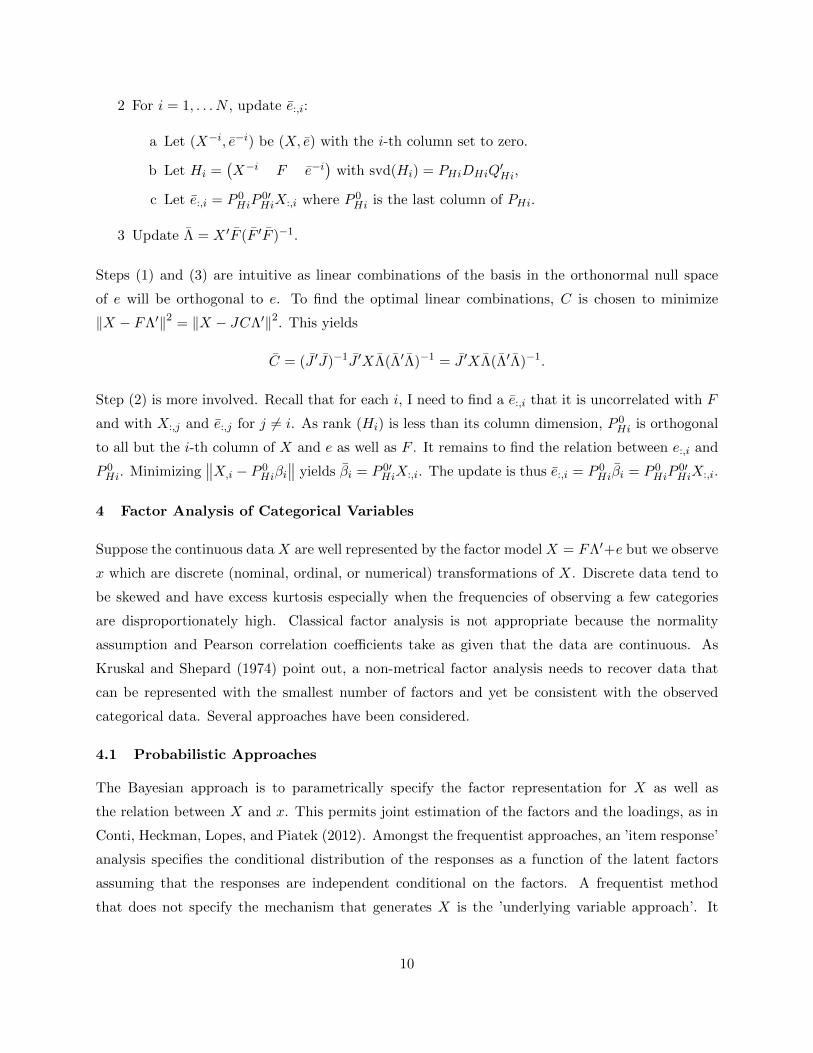
2 For i = 1, . . . N , update e:,i:

a Let (X−i, e−i) be (X, e) with the i-th column set to zero.

b Let Hi =(X−i F e−i

)with svd(Hi) = PHiDHiQ

′Hi,

c Let e:,i = P 0HiP

0′HiX:,i where P 0

Hi is the last column of PHi.

3 Update Λ = X ′F (F ′F )−1.

Steps (1) and (3) are intuitive as linear combinations of the basis in the orthonormal null space

of e will be orthogonal to e. To find the optimal linear combinations, C is chosen to minimize

‖X − FΛ′‖2 = ‖X − JCΛ′‖2. This yields

C = (J ′J)−1J ′XΛ(Λ′Λ)−1 = J ′XΛ(Λ′Λ)−1.

Step (2) is more involved. Recall that for each i, I need to find a e:,i that it is uncorrelated with F

and with X:,j and e:,j for j 6= i. As rank (Hi) is less than its column dimension, P 0Hi is orthogonal

to all but the i-th column of X and e as well as F . It remains to find the relation between e:,i and

P 0Hi. Minimizing

∥∥X,i − P 0Hiβi

∥∥ yields βi = P 0′HiX:,i. The update is thus e:,i = P 0

Hiβi = P 0HiP

0′HiX:,i.

4 Factor Analysis of Categorical Variables

Suppose the continuous data X are well represented by the factor model X = FΛ′+e but we observe

x which are discrete (nominal, ordinal, or numerical) transformations of X. Discrete data tend to

be skewed and have excess kurtosis especially when the frequencies of observing a few categories

are disproportionately high. Classical factor analysis is not appropriate because the normality

assumption and Pearson correlation coefficients take as given that the data are continuous. As

Kruskal and Shepard (1974) point out, a non-metrical factor analysis needs to recover data that

can be represented with the smallest number of factors and yet be consistent with the observed

categorical data. Several approaches have been considered.

4.1 Probabilistic Approaches

The Bayesian approach is to parametrically specify the factor representation for X as well as

the relation between X and x. This permits joint estimation of the factors and the loadings, as in

Conti, Heckman, Lopes, and Piatek (2012). Amongst the frequentist approaches, an ’item response’

analysis specifies the conditional distribution of the responses as a function of the latent factors

assuming that the responses are independent conditional on the factors. A frequentist method

that does not specify the mechanism that generates X is the ’underlying variable approach’. It

10

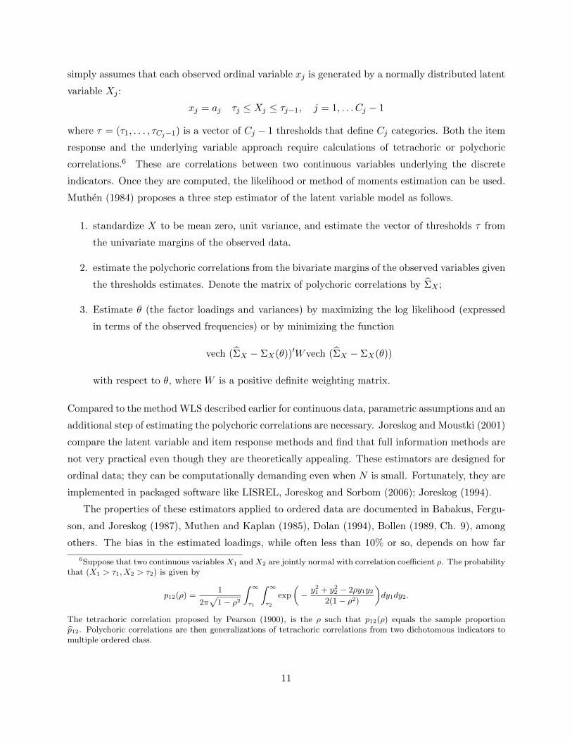
simply assumes that each observed ordinal variable xj is generated by a normally distributed latent

variable Xj :

xj = aj τj ≤ Xj ≤ τj−1, j = 1, . . . Cj − 1

where τ = (τ1, . . . , τCj−1) is a vector of Cj − 1 thresholds that define Cj categories. Both the item

response and the underlying variable approach require calculations of tetrachoric or polychoric

correlations.6 These are correlations between two continuous variables underlying the discrete

indicators. Once they are computed, the likelihood or method of moments estimation can be used.

Muthen (1984) proposes a three step estimator of the latent variable model as follows.

1. standardize X to be mean zero, unit variance, and estimate the vector of thresholds τ from

the univariate margins of the observed data.

2. estimate the polychoric correlations from the bivariate margins of the observed variables given

the thresholds estimates. Denote the matrix of polychoric correlations by ΣX ;

3. Estimate θ (the factor loadings and variances) by maximizing the log likelihood (expressed

in terms of the observed frequencies) or by minimizing the function

vech (ΣX − ΣX(θ))′Wvech (ΣX − ΣX(θ))

with respect to θ, where W is a positive definite weighting matrix.

Compared to the method WLS described earlier for continuous data, parametric assumptions and an

additional step of estimating the polychoric correlations are necessary. Joreskog and Moustki (2001)

compare the latent variable and item response methods and find that full information methods are

not very practical even though they are theoretically appealing. These estimators are designed for

ordinal data; they can be computationally demanding even when N is small. Fortunately, they are

implemented in packaged software like LISREL, Joreskog and Sorbom (2006); Joreskog (1994).

The properties of these estimators applied to ordered data are documented in Babakus, Fergu-

son, and Joreskog (1987), Muthen and Kaplan (1985), Dolan (1994), Bollen (1989, Ch. 9), among

others. The bias in the estimated loadings, while often less than 10% or so, depends on how far

6Suppose that two continuous variables X1 and X2 are jointly normal with correlation coefficient ρ. The probabilitythat (X1 > τ1, X2 > τ2) is given by

p12(ρ) =1

2π√

1 − ρ2

∫ ∞τ1

∫ ∞τ2

exp

(− y21 + y22 − 2ρy1y2

2(1 − ρ2)

)dy1dy2.

The tetrachoric correlation proposed by Pearson (1900), is the ρ such that p12(ρ) equals the sample proportionp12. Polychoric correlations are then generalizations of tetrachoric correlations from two dichotomous indicators tomultiple ordered class.

11

are the categorized data from normality. Furthermore, the covariance matrix of the estimated id-

iosyncratic errors often have non-zero off-diagonal entries even if the true idiosyncratic errors are

mutually uncorrelated. The possibility that categorical data may lead to spurious factors has also

been raised, McDonald (1985, Ch. 4).

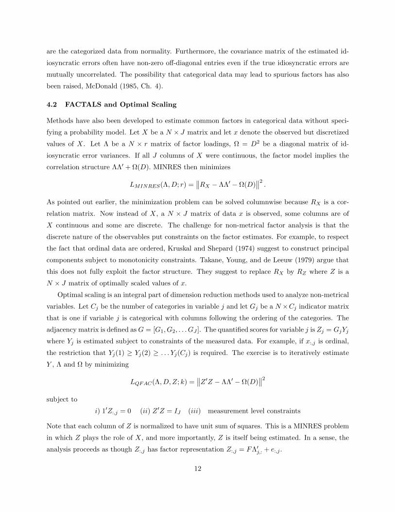
4.2 FACTALS and Optimal Scaling

Methods have also been developed to estimate common factors in categorical data without speci-

fying a probability model. Let X be a N × J matrix and let x denote the observed but discretized

values of X. Let Λ be a N × r matrix of factor loadings, Ω = D2 be a diagonal matrix of id-

iosyncratic error variances. If all J columns of X were continuous, the factor model implies the

correlation structure ΛΛ′ + Ω(D). MINRES then minimizes

LMINRES(Λ, D; r) =∥∥RX − ΛΛ′ − Ω(D)

∥∥2 .As pointed out earlier, the minimization problem can be solved columnwise because RX is a cor-

relation matrix. Now instead of X, a N × J matrix of data x is observed, some columns are of

X continuous and some are discrete. The challenge for non-metrical factor analysis is that the

discrete nature of the observables put constraints on the factor estimates. For example, to respect

the fact that ordinal data are ordered, Kruskal and Shepard (1974) suggest to construct principal

components subject to monotonicity constraints. Takane, Young, and de Leeuw (1979) argue that

this does not fully exploit the factor structure. They suggest to replace RX by RZ where Z is a

N × J matrix of optimally scaled values of x.

Optimal scaling is an integral part of dimension reduction methods used to analyze non-metrical

variables. Let Cj be the number of categories in variable j and let Gj be a N ×Cj indicator matrix

that is one if variable j is categorical with columns following the ordering of the categories. The

adjacency matrix is defined asG = [G1, G2, . . . GJ ]. The quantified scores for variable j is Zj = GjYj

where Yj is estimated subject to constraints of the measured data. For example, if x:,j is ordinal,

the restriction that Yj(1) ≥ Yj(2) ≥ . . . Yj(Cj) is required. The exercise is to iteratively estimate

Y , Λ and Ω by minimizing

LQFAC(Λ, D, Z; k) =∥∥Z ′Z − ΛΛ′ − Ω(D)

∥∥2subject to

i) 1′Z:,j = 0 (ii) Z ′Z = IJ (iii) measurement level constraints

Note that each column of Z is normalized to have unit sum of squares. This is a MINRES problem

in which Z plays the role of X, and more importantly, Z is itself being estimated. In a sense, the

analysis proceeds as though Z:,j has factor representation Z:,j = FΛ′j,: + e:,j .

12

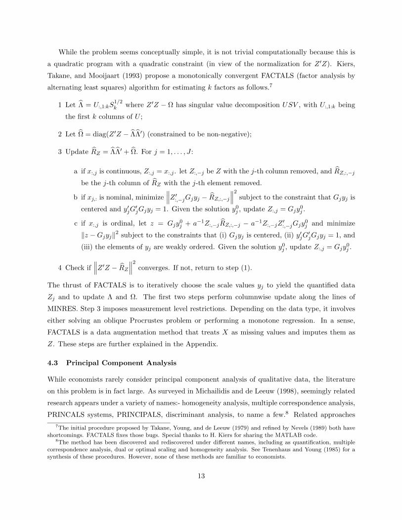
While the problem seems conceptually simple, it is not trivial computationally because this is

a quadratic program with a quadratic constraint (in view of the normalization for Z ′Z). Kiers,

Takane, and Mooijaart (1993) propose a monotonically convergent FACTALS (factor analysis by

alternating least squares) algorithm for estimating k factors as follows.7

1 Let Λ = U:,1:kS1/2k where Z ′Z − Ω has singular value decomposition USV , with U:,1:k being

the first k columns of U ;

2 Let Ω = diag(Z ′Z − ΛΛ′) (constrained to be non-negative);

3 Update RZ = ΛΛ′ + Ω. For j = 1, . . . , J :

a if x:,j is continuous, Z:,j = x:,j . let Z:,−j be Z with the j-th column removed, and RZ,:,−j

be the j-th column of RZ with the j-th element removed.

b if xj,: is nominal, minimize∥∥∥Z ′:,−jGjyj − RZ,:,−j∥∥∥2 subject to the constraint that Gjyj is

centered and y′jG′jGjyj = 1. Given the solution y0j , update Z:,j = Gjy

0j .

c if x:,j is ordinal, let z = Gjy0j + a−1Z:,−jRZ,:,−j − a−1Z:,−jZ

′:,−jGjy

0j and minimize

‖z −Gjyj‖2 subject to the constraints that (i) Gjyj is centered, (ii) y′jG′jGjyj = 1, and

(iii) the elements of yj are weakly ordered. Given the solution y0j , update Z:,j = Gjy0j .

4 Check if∥∥∥Z ′Z − RZ∥∥∥2 converges. If not, return to step (1).

The thrust of FACTALS is to iteratively choose the scale values yj to yield the quantified data

Zj and to update Λ and Ω. The first two steps perform columnwise update along the lines of

MINRES. Step 3 imposes measurement level restrictions. Depending on the data type, it involves

either solving an oblique Procrustes problem or performing a monotone regression. In a sense,

FACTALS is a data augmentation method that treats X as missing values and imputes them as

Z. These steps are further explained in the Appendix.

4.3 Principal Component Analysis

While economists rarely consider principal component analysis of qualitative data, the literature

on this problem is in fact large. As surveyed in Michailidis and de Leeuw (1998), seemingly related

research appears under a variety of names:- homogeneity analysis, multiple correspondence analysis,

PRINCALS systems, PRINCIPALS, discriminant analysis, to name a few.8 Related approaches

7The initial procedure proposed by Takane, Young, and de Leeuw (1979) and refined by Nevels (1989) both haveshortcomings. FACTALS fixes those bugs. Special thanks to H. Kiers for sharing the MATLAB code.

8The method has been discovered and rediscovered under different names, including as quantification, multiplecorrespondence analysis, dual or optimal scaling and homogeneity analysis. See Tenenhaus and Young (1985) for asynthesis of these procedures. However, none of these methods are familiar to economists.

13

also include the principal factor analysis of Keller and Wansbeek (1983) and redudancy analysis

(canonical correlation) of Israels (1984). As with continuous data, principal component analysis

differs from factor analysis by going a step further to impose a structure.

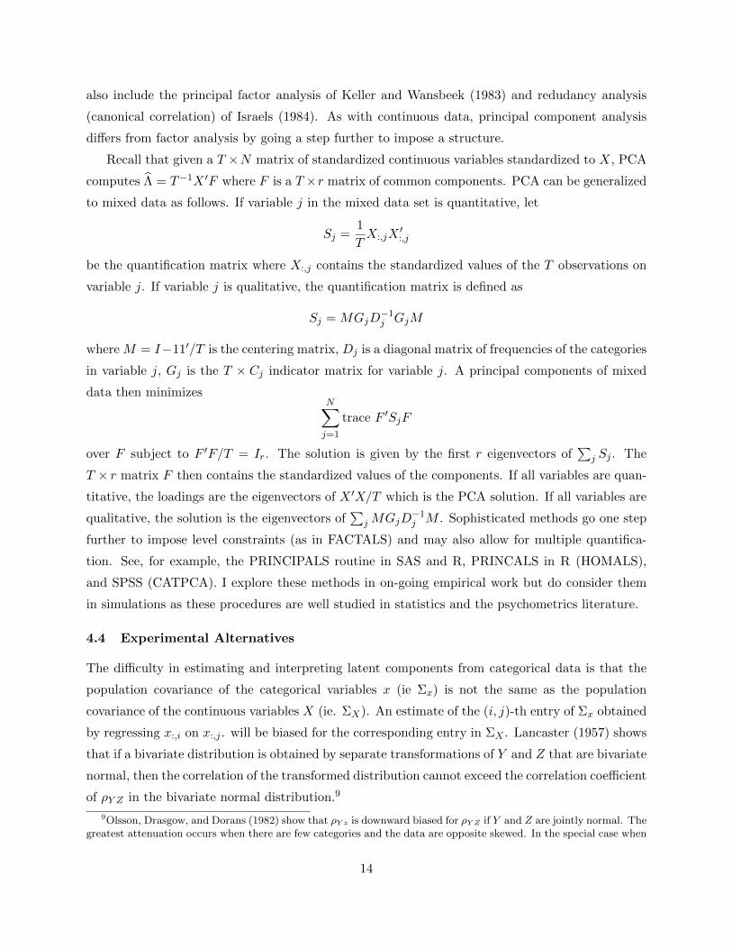
Recall that given a T ×N matrix of standardized continuous variables standardized to X, PCA

computes Λ = T−1X ′F where F is a T ×r matrix of common components. PCA can be generalized

to mixed data as follows. If variable j in the mixed data set is quantitative, let

Sj =1

TX:,jX

′:,j

be the quantification matrix where X:,j contains the standardized values of the T observations on

variable j. If variable j is qualitative, the quantification matrix is defined as

Sj = MGjD−1j GjM

where M = I−11′/T is the centering matrix, Dj is a diagonal matrix of frequencies of the categories

in variable j, Gj is the T × Cj indicator matrix for variable j. A principal components of mixed

data then minimizesN∑j=1

trace F ′SjF

over F subject to F ′F/T = Ir. The solution is given by the first r eigenvectors of∑

j Sj . The

T × r matrix F then contains the standardized values of the components. If all variables are quan-

titative, the loadings are the eigenvectors of X ′X/T which is the PCA solution. If all variables are

qualitative, the solution is the eigenvectors of∑

jMGjD−1j M . Sophisticated methods go one step

further to impose level constraints (as in FACTALS) and may also allow for multiple quantifica-

tion. See, for example, the PRINCIPALS routine in SAS and R, PRINCALS in R (HOMALS),

and SPSS (CATPCA). I explore these methods in on-going empirical work but do consider them

in simulations as these procedures are well studied in statistics and the psychometrics literature.

4.4 Experimental Alternatives

The difficulty in estimating and interpreting latent components from categorical data is that the

population covariance of the categorical variables x (ie Σx) is not the same as the population

covariance of the continuous variables X (ie. ΣX). An estimate of the (i, j)-th entry of Σx obtained

by regressing x:,i on x:,j . will be biased for the corresponding entry in ΣX . Lancaster (1957) shows

that if a bivariate distribution is obtained by separate transformations of Y and Z that are bivariate

normal, then the correlation of the transformed distribution cannot exceed the correlation coefficient

of ρY Z in the bivariate normal distribution.9

9Olsson, Drasgow, and Dorans (1982) show that ρY z is downward biased for ρY Z if Y and Z are jointly normal. Thegreatest attenuation occurs when there are few categories and the data are opposite skewed. In the special case when

14

In fact, discretization is a form of data transformation that is known to underestimate the

linear relation between two variables though the problem is alleviated as the number of categories

increases. As mentioned earlier, many simulation studies have found that the r factor loadings

estimated by MLE and WLS do not behave well when the data exhibit strongly non-Gaussian

features. Data transformations can induce such features. But as seen above, estimating latent

components from discrete data is quite not a trivial task.

A practical approach that has gained popularity in analysis of socio-economic data is the so-

called Filmer-Pritchett method used in Filmer and Pritchett (1998). Essentially, the method con-

structs principal components from the adjacency matrix, G. Kolenikov and Angeles (2009) assess

the model’s predicted rankings and find the method to be inefficient because it loses the ordinal

information in the data. Furthermore, spurious negative correlation in the G matrix could under-

estimate the common variations in the data. However, they also find that constructing principal

components from polychoric correlations of socio-economic data did not yield substantial improve-

ments over the Filmer-Pritchett method.

I explore two alternatives that seem sensible when structural interpretation of the components

in categorical variable is not necessary, and that N is large. The hope is that in such cases (as

in economic forecasting), simpler procedures can be used to extract information in the categorical

variables. The first idea is to construct the principal components from the quantified data. If

principal components precisely estimates the space spanned by X, and Z are good quantifications

of the discrete data x, then PCA applied to Z should estimate the space spanned by the common

factors in X. I therefore obtain the quantified data Z by FACTALS and then apply PCA to the

covariance of Z (ie. RZ

) to obtain estimate F and Λ. The approach is a natural generalization

of the method of asymptotic principal components used when X was observed. However, the Λ

estimated by PCA applied to Z will generally be different from those that directly emerge from

FACTALS because PCA does not impose diagonality of Ω. It will also be different from the ones

that emerge from homogeneity analysis because level constraints are not imposed.

The second method is to ignore the fact that some variables are actually discrete and to extract

principal components of Σx. As pointed out earlier, the eigenvectors of X will generally be different

from those of x because ΣX 6= Σx. In a sense, x is a contaminated copy of X. The hope is that the

salient information in X will be retained in a sufficiently large number of eigenvectors of x, and

that principal components will be able to extract this information. In other words, I compensate

for the information loss created by data transformations with more latent components than would

otherwise be used if X was observed.

consecutive integers are assigned to categories of Y , it can be shown that ρY z = ρY Z ·q, where q = 1σθ

∑J−1j=1 φ(αj)

and φ(·) is the standard normal density and q is the categorization attenuation factor.

15

5 Monte Carlo Simulations

This section has two parts. The first subsection focuses on continuous data and assesses the precision

of the factor estimates produced by the method of asymptotic principal components, ALS1, and

ALS2. I also evaluate criterion for determining the number of factors. Subsection two turns to

categorical and mixed data. All computations are based on MATLAB Release 2011a.

5.1 Continuous Data

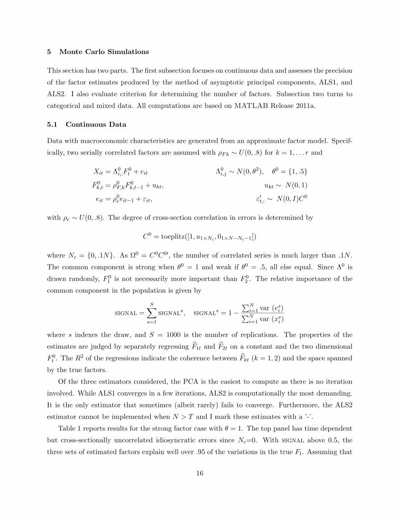
Data with macroeconomic characteristics are generated from an approximate factor model. Specif-

ically, two serially correlated factors are assumed with ρFk ∼ U(0, .8) for k = 1, . . . r and

Xit = Λ0i,:F

0t + eit Λ0

i,j ∼ N(0, θ2), θ0 = 1, .5

F 0k,t = ρ0F,kF

0k,t−1 + ukt, ukt ∼ N(0, 1)

eit = ρ0eeit−1 + εit, ε′t,: ∼ N(0, I)C0

with ρe ∼ U(0, .8). The degree of cross-section correlation in errors is deteremined by

C0 = toeplitz([1, u1×Nc , 01×N−Nc−1])

where Nc = 0, .1N. As Ω0 = C0C0′, the number of correlated series is much larger than .1N .

The common component is strong when θ0 = 1 and weak if θ0 = .5, all else equal. Since Λ0 is

drawn randomly, F 01 is not necessarily more important than F 0

2 . The relative importance of the

common component in the population is given by

signal =S∑s=1

signals, signals = 1−∑N

i=1 var (esi )∑Ni=1 var (xsi )

where s indexes the draw, and S = 1000 is the number of replications. The properties of the

estimates are judged by separately regressing F1t and F2t on a constant and the two dimensional

F 0t . The R2 of the regressions indicate the coherence between Fkt (k = 1, 2) and the space spanned

by the true factors.

Of the three estimators considered, the PCA is the easiest to compute as there is no iteration

involved. While ALS1 converges in a few iterations, ALS2 is computationally the most demanding.

It is the only estimator that sometimes (albeit rarely) fails to converge. Furthermore, the ALS2

estimator cannot be implemented when N > T and I mark these estimates with a ’-’.

Table 1 reports results for the strong factor case with θ = 1. The top panel has time dependent

but cross-sectionally uncorrelated idiosyncratic errors since Nc=0. With signal above 0.5, the

three sets of estimated factors explain well over .95 of the variations in the true Ft. Assuming that

16

eit is cross-sectionally uncorrelated did not hurt the efficiency of PCA because the constraint is

correct in this case.

The bottom panel of Table 1 allows the errors to be cross-sectionally correlated. As a con-

sequence, the common component relative to the total variation in the data falls by as much as

half. Notably, all factor estimates are less precise. One PCA factor tends to be more precisely

estimated than the other. The discrepancy seems to increase as signal decreases. The two ALS

estimators are much more even in this regard since F1 and F2 have similar predictive power of the

factor space. Of the three estimators, ALS2 appears to be most unstable; it can be extremely good

(such as when (T,N) = (120, 80)) or extremely bad (such as when T is increased to 240) holding

Nc fixed at =8. A factor that is precisely estimated by the PCA is not always precisely estimated

by the ALS estimators and vice versa. When (T,N) = (240, 120), F 01 is poorly estimated by the

ALS estimators (R2 of .111 and .272) than by PCA (with R2 of .524). However, the reverse is true

of F 02 , with R2 of .824 and .739 for the ALS estimators, and only .355 for the PCA.

Table 2 considers weaker factor loadings with θ = 0.5. When the errors are not cross-sectionally

correlated, signal in the top panel of Table 2 is reduced somewhat relative to Table 1 but the

correlation is not enough to strongly affect the precision of the factor estimates. For example, when

(T,N) = (120, 40), R2 is 0.960 when θ = 1 and is 0.865 when θ = .5. When (T,N) = (40, 120), R2

goes from .987 to 0.94. When the idiosyncratic errors are also cross-sectionally correlated, the drop

in signal is much larger. The R2 values in the second panel of Table 2 are one-third to one-quarter

of those in Table 1. Weak loadings combined with cross-correlated errors drastically reduce the

precision of the factor estimates irrespective of the method used. When (T,N) = (240, 120) which

is not an unusual configuration of the data encountered in practice, signal falls from .254 to .078

and the average R2 drops from around .5 in Table 1 to less than .05 in Table 2! The difference is

attributed to cross-correlated errors.

The results in Tables 1 and 2 are based on the assumption that r is known. Bai and Ng (2002)

show that the number of factors can be consistently estimated by minimizing LPCA subject to the

constraint of parsimony. Specifically,

rPCA = argmink=kmin,...,kmax

logLPCA(k) + kg(N,T )

where g(N,T ) → 0 but min(N,T )g(N,T ) → ∞. The ALS estimators are based on different

objective functions. While their statistical properties are not known, Tables 1 and 2 find that the

estimated ALS factors behave similarly to the PCA ones. I therefore let

rALS = argmink=kmin,...,kmax

logLALS(k)/nT + kg(N,T ).

17

In the simulations, I use

g2(N,T ) =N + T

NTlog min(N,T )

noting that NT/(N + T ) ≈ min(N,T )−1. This corresponds to IC2 recommended in Bai and Ng

(2008). For the ALS estimators I also consider a heavier penalty

gA(N,T ) =N + T

NTlog(N · T ).

The simulation design is similar to Tables 1 and 2. The criteria are evaluated for k = 0, . . . , 6.

I only consider 500 replications because ALS2 is extremely time consuming to compute. The

results are reported in Table 3. When θ = 1 and the errors are cross-sectionally uncorrelated, the

IC2 almost always chooses the correct number of factors. The suitably penalized ALS objective

functions also give the correct number of factors. The estimates of r are imprecise when there

is cross-section dependence in eit. The g2 penalty often chooses the maximum number of factors

whether PCA or ALS is used to estimate F , while the gA tends to select too few factors. The

results are to be expected; the penalties developed in Bai and Ng (2002) are predicated on a strong

factor structure with weakly correlated idiosyncratic errors. When those assumptions are violated,

the penalties are no longer appropriate.

The AO criterion of Onatski (2010) is supposed to better handle situations when there is

substantial correlation in the errors. As seen from the third panel of Table 3, the AO criterion

gives more precise estimates of r when the factor loadings are weak. However, it tends to select

zero factors when many of the idiosyncratic errors are cross-sectionally correlated. Onatski (2010)

argues that his criterion selects the number of factors that can be consistently estimated. It is

not surprising that the AO criterion selects fewer factors when the factor component is weak. But

taking the argument at face value would suggest that when signal is below .3, none of the two

factors can be consistently estimated by the PCA or the ALS. This seems at odds with the fact

that the estimated factors still have substantial correlation with the true factors.

Two conclusions can be drawn from these simulations. First, the objective function used to

obtain F seems to make little difference as the PCA and ALS estimates are similar. Second, not

constraining Ω to be diagonal (as in the PCA) or unnecessarily imposing the constraint (as in the

ALS) also does not have much effect on R2. In this regard, the results echo those of Doz, Giannone,

and Reichlin (2007). If the strong factor assumptions hold true, there is little to choose between

the estimators on the basis of the precise estimation of the factor space. Nonetheless, the PCA is

computationally much less demanding.

Second, the precision of the factor estimates are strongly influenced by weak factor loadings.

While signal is not observed and it is not known if the factors are strong or weak in practice, two

indicators can be useful. The first is R2 which should increase with signal. A low R2 in spite

18

of using many factors would be a cause for concern. The second is the discrepancy between the

number of factors selected by IC2 and AO. The two estimates should not be far apart when the

factor structure is strong. When the rs are very different, the strong factor assumptions may be

questionable.

5.2 Mixed Data

Two designs of categorical data are considered. In the first case, the ordinal data x consists of

answers by N respondents (such as professional forecasters) to the same question (such as whether

they expect inflation to go up, down, or stay the same) over time T periods. In the second case,

x consists of J responses (such as on income and health status) for each of the N units (such as

households). In these experiments, PCA is used to estimate r factors in (i) the continuous data

X as if it were observed, (ii) the categorical data x, (iii) the adjacency matrix G, and (where

appropriate) (iv) the quantified data Z. The number of factors is determined by the criterion in

Bai and Ng (2002) with penalty g2 or the AO test of Onatski (2010). I begin with the first case

when all data are ordinal.

a) PCA of X, x : and G Data on one variable X are generated for N units for T time periods.

The J − 1 thresholds are evenly spaced and are generated using norminv(.05:J-1:.95). The data

matrix is first standardized columnwise and then categorized into x which has J groups.

The results are given in Table 4. Columns 3 and 4 show that if X was observed, the number

of factors would be precisely estimated. As seen from column 5 and 6, r remains fairly precisely

estimated when the categorical data x are used instead of X. However, the estimated number of

factors in the adjacency matrix G is less stable. There are too few factors when the sample size is

small but too many factors when N and T are large.10

Turning to an assessment of the estimated factor space, R2X indicates the average R2 when

r principal components are estimated from X where the r is determined by penalty g2. The

interpretation is similar for R2x and R2

G. Evidently, F precisely estimates F when X was available

for analysis. The R2s are slightly lower if the factors are estimated from x but the difference is

quite small. The average R2 remains well over .95. However, the principal components of the

adjacency matrix G are less informative about the true factors. When the sample size is small and

r underestimates r, R2G can be much lower than R2

x. For example, when r = 2, R2x is .916 when

(T,N) = (100, 20), but R2G is only .368. The situation improves when the sample size increases

as estimating more factors in G compensates for the information loss in the indicator variables.

10In an earlier version of the paper when x and G were not demeaned, PCA estimated one more factor in both xand G.

19

However, even with large r, the principal components of G remain less informative about F 0 than

the principal components of x. When (T,N) = (200, 100), R2x is .956 while R2

G is .849, even though

on average, r = 3 > r = 2 factors are found in G.

b) PCA of X, x, G and Z Data for J variables for each of the N units are generated as:

Xij = Λ0i,:F

0t + eij

where eij ∼ N(0, σ2), Λ0i,: is a 1× r vector of standard normal variates, F 0

t ∼ N(0, Ir). The factor

loadings are N(0, θ2). The J continuous variables are categorized using unevenly spaced thresholds

as summarized in the bottom of Table 5. The total number of categories (also the dimension of G)

is denoted nG.

The results for the case of strong loadings (θ = 1) are in the top panel of Table 5. As seen

from columns 5 to 8, the number of factors is overestimated whenever J is small even if X was

observed; the average R2 is .75 when J is 5 but increases to .941 when J = 30. This just shows

that principal components can precisely estimate the factor space only when J is reasonably large.

There is undoubtedly a loss of precision when X is not observed. The principal components of G

yield low R2 for small values of J . Apparently, G contains less information about F than Z. While

the number of factors found in the discrete data x exceeds r, the r principal components of x give

R2s close to those based on Z. In other words, with enough estimated factors, the factor space can

be as precisely estimated from discrete data than as from the quantified data.

The lower panel of Table 5 are results for the case of weak loadings with θ = .5. Now R2Z and

R2G are much reduced as the corresponding number of factors found in Z and G tends to be below

the true value of two. This suggests that when the factor structure is already weak, discretization

further weakens the information about the common factors in x. It is thus difficult to recover F

from quantified data or from transformations of x. In such a case, the principal components of the

raw categorical data x give the most precise factor estimates and they are easiest to construct.

The final set of simulations consider mixed continuous, nominal and ordinal data. The number

of continuous variables is always 20, the number of nominal variables Jnominal is either 5 or 10, and

the number of ordinal variables Jordinal is 5, 10, or 20.11 The results are given in Table 6. The

number of factors is correctly estimated from the continuous data X, the quantified data Z, or

the discrete data x but are overestimated from the dummy variable matrix G. The factor space is

precisely estimated using X, Z or x but not G. The results are similar to those for purely ordinal

data.

11The FACTALS has convergence problems when N is 100 and the dimension of G is large.

20

6 Conclusion

This paper reviews and explores various matrix decomposition based methods for estimating the

common factors in mixed data. A few conclusions can be drawn. First, if all data are continuous

and T and N are large, ALS estimators have no significant advantage over PCA which is much

simpler to construct. Second, with mixed data, the principal components of G give the least precise

estimates of the factor space. Third, FACTALS provides a way to quantify the data consistent with

a factor structure. But while the factor space can be precisely obtained from Z when the factor

structure is strong, they are no more precise than analyzing x directly, and it is not robust when

the factor structure in X is weak. Fourth, the observed categorical data x can be used to estimate

the factor space quite precisely though additional factors may be necessary to compensate for the

information that is lost from data discretization. It should be emphasized that different conclusions

might emerge if criterion other than the factor space is used. Furthermore, the Monte Carlo exercise

is quite limited in scope. Nonetheless, the findings are encouraging and merit further investigation.

I consider FACTALS because it constructs quantified data Z consistent with a factor structure

which allows me to consider a large dimensional factor analysis treating Z as data. However, as

pointed out earlier, the sample correlations of transformed data are not the same as the raw data.

Nothing ensures that Z will necessarily recover X from x. Thus, an important caveat of non-

metrical factor analysis is that Z may not be unique even when its second moments are consistent

with the factor structure implied by the data X. Buja (1990) warns that the transformed data may

identify spurious structures because singular values are sensitive to small changes in the data. A

better understanding of these issues is also necessary.

21

7 Appendix

This appendix elaborates on how nominal and ordinal data are optimally scaled. It will be seen

that the steps rely on matrix arguments presented in Section 3.

Step 3b: Nominal Variables Observe first that Z ′:,−jGjyj = Z ′:,−jZ:,j defines the vector of

’sample’ cross correlations, while RZ,−j is the model implied analog. The j-entry is omitted since

it is one by construction in both the sample and the model. We put sample in quotes because Z

are quantified variables and not data.

Let M = IT − 11′/T be the idempotent matrix that demeans the data. Constraining Z to be

mean zero columnwise is equivalent to imposing the condition MGjyj = Gjyj for every j with

Z ′:,−jGjyj = Z ′:,−jMGjyj . Let B be an orthonormal bases for MGjyj . Then MGjyj = Bτ for some

τ . Instead of minimizing∥∥∥Z ′:,−jGjyj − RZ,:,−j∥∥∥2 over yj subject to the constraint y′jG

′jGjyj =

y′jG′jMGjyj , the problem is now to minimize∥∥∥Z ′−j,:Bτ − RZ,:,−j∥∥∥2

over τ subject to the constraint that τ ′B′Bτ = τ ′τ = 1. This is an oblique Mosier’s Procrustes

problem whose solution, denoted τ0, is given in Cliff (1966) and ten Berge and Nevels (1997). Given

τ0, yj can be solved from MGjyj = Bτ0. By least squares argument,

y0j = (G′jGj)−1G′jBτ0.

It remains to explain the oblique Procrustes problem. Recall that the orthogonal Procrustes

problem looks for a m × k transformation matrix B to minimize ‖Λ−AB‖2 subject to B′B = I.

The oblique Procrustes problem imposes the constraint diag(B′B) = I. Since the constraint is now

a diagonal matrix, each column of B can be solved separately. Let β be a vector from B, and λ

be a column of Λ. The objective is now to find β to minimize (λ−Aβ)′(λ−Aβ). For U such that

UU ′ = U ′U = I and A′A = UCU ′, the problem can be rewritten as

(λ−Aβ)′(λ−Aβ) = (λ−AUβ)′(λ−AUβ).

By letting w = U ′β and x = U ′Aλ, the problem is equivalent to finding a vector w to minimize

λ′λ− 2x′w + w′Cw subject to w′w = 1.

The objective function and the constraint are both in quadratic form. The (non-linear) solution

depends on q, the multiplicity of the smallest latent root of A′A. In the simulations, I use the

algorithm of ten Berge and Nevels (1997). In the present problem, λ = RZ,:,−j and A = Z ′:,−jB.

22

Step 3c: Ordinal Variables When X:,j is ordinal, we minimize a function that majorizes f(yj)

and whose solution is easier to find. As shown in Kiers (1990), this is accomplished by viewing f

as a function of q = Gjyj . The function of interest (for given q0)

f(q) =∥∥∥Z ′:,−jq − RZ,:,−j∥∥∥ = R′Z,:,−jRZ,:,−j − 2R′Z,:,−jZ

′:,−jq + trace (Z:,−jZ

′:,−jqq

′)

is majorized by

g(q) = c1 + a

(∥∥∥q0 − (2a)−1(−2Z:,−jRZ,:,−j + 2Z:,−jZ′:,−jq

0)− q∥∥∥2 + c2

)where c1 and c2 are constants for q, and a is the first eigenvalue of Z:,−jZ

′:,−j . Re-expressing qj in

terms of Gjyj , we can maximize

h(yj) =∥∥∥Gjy0j − (2a)−1(−2Z:,−jRZ,:,−j + 2Z:,−jZ

′:,−jGjG

0j )−Gjyj

∥∥∥2=

∥∥∥(Gjy0j + a−1Z:,−jRZ,:,−j − a−1Z:,−jZ

′:,−jGjy

0j )−Gjyj

∥∥∥2= ‖z −Gjyj‖2

subject to the constraints that Gjyj is centered and y′jG′jGjyj = 1. This is now a normalized

monotone regression problem.12

12Given weights w1, . . . , wT and real numbers x1, . . . , xT , the monotone (isotonic) regression problem finds x1, . . . xTto minimize S(y) =

∑Tt=1 wt(xt − yt)

2 subject to the monotonicity condition t k implies yt ≤ yk where is apartial ordering on the index set [1, . . . T ]. An up-and-down-block algorithm is given in Kruskal (1964). See alsode Leeuw (2005).

23

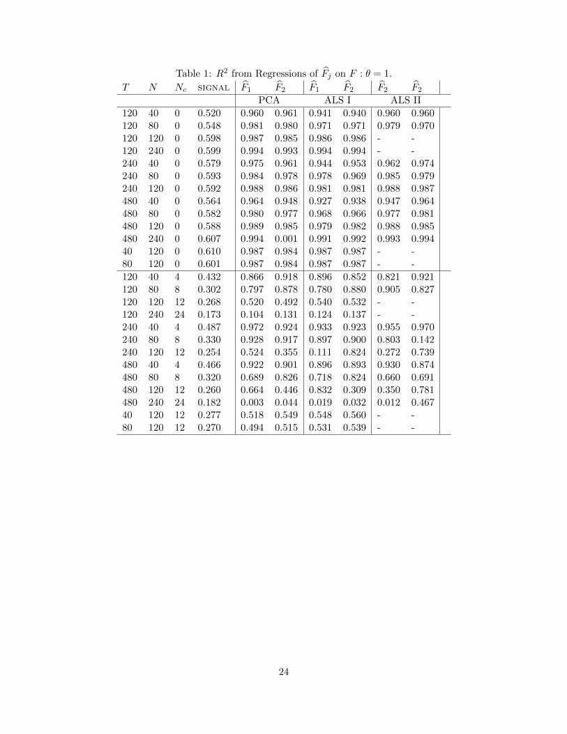
Table 1: R2 from Regressions of Fj on F : θ = 1.

T N Nc signal F1 F2 F1 F2 F2 F2

PCA ALS I ALS II

120 40 0 0.520 0.960 0.961 0.941 0.940 0.960 0.960120 80 0 0.548 0.981 0.980 0.971 0.971 0.979 0.970120 120 0 0.598 0.987 0.985 0.986 0.986 - -120 240 0 0.599 0.994 0.993 0.994 0.994 - -240 40 0 0.579 0.975 0.961 0.944 0.953 0.962 0.974240 80 0 0.593 0.984 0.978 0.978 0.969 0.985 0.979240 120 0 0.592 0.988 0.986 0.981 0.981 0.988 0.987480 40 0 0.564 0.964 0.948 0.927 0.938 0.947 0.964480 80 0 0.582 0.980 0.977 0.968 0.966 0.977 0.981480 120 0 0.588 0.989 0.985 0.979 0.982 0.988 0.985480 240 0 0.607 0.994 0.001 0.991 0.992 0.993 0.99440 120 0 0.610 0.987 0.984 0.987 0.987 - -80 120 0 0.601 0.987 0.984 0.987 0.987 - -

120 40 4 0.432 0.866 0.918 0.896 0.852 0.821 0.921120 80 8 0.302 0.797 0.878 0.780 0.880 0.905 0.827120 120 12 0.268 0.520 0.492 0.540 0.532 - -120 240 24 0.173 0.104 0.131 0.124 0.137 - -240 40 4 0.487 0.972 0.924 0.933 0.923 0.955 0.970240 80 8 0.330 0.928 0.917 0.897 0.900 0.803 0.142240 120 12 0.254 0.524 0.355 0.111 0.824 0.272 0.739480 40 4 0.466 0.922 0.901 0.896 0.893 0.930 0.874480 80 8 0.320 0.689 0.826 0.718 0.824 0.660 0.691480 120 12 0.260 0.664 0.446 0.832 0.309 0.350 0.781480 240 24 0.182 0.003 0.044 0.019 0.032 0.012 0.46740 120 12 0.277 0.518 0.549 0.548 0.560 - -80 120 12 0.270 0.494 0.515 0.531 0.539 - -

24

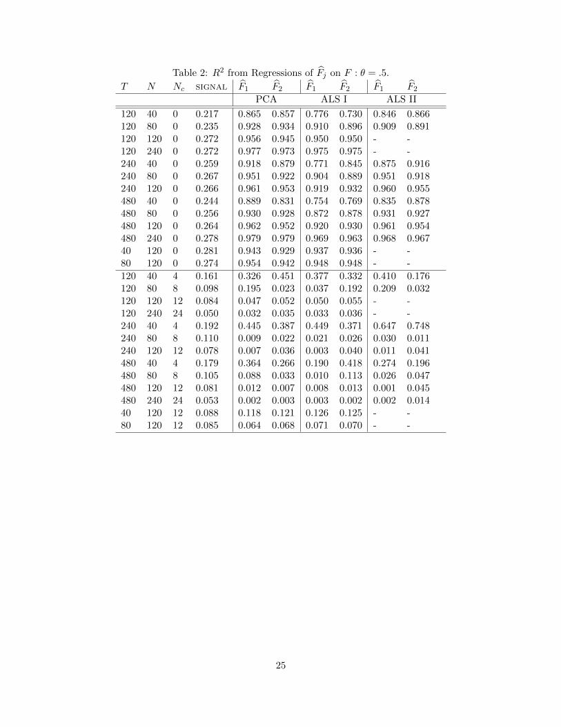
Table 2: R2 from Regressions of Fj on F : θ = .5.

T N Nc signal F1 F2 F1 F2 F1 F2

PCA ALS I ALS II

120 40 0 0.217 0.865 0.857 0.776 0.730 0.846 0.866120 80 0 0.235 0.928 0.934 0.910 0.896 0.909 0.891120 120 0 0.272 0.956 0.945 0.950 0.950 - -120 240 0 0.272 0.977 0.973 0.975 0.975 - -240 40 0 0.259 0.918 0.879 0.771 0.845 0.875 0.916240 80 0 0.267 0.951 0.922 0.904 0.889 0.951 0.918240 120 0 0.266 0.961 0.953 0.919 0.932 0.960 0.955480 40 0 0.244 0.889 0.831 0.754 0.769 0.835 0.878480 80 0 0.256 0.930 0.928 0.872 0.878 0.931 0.927480 120 0 0.264 0.962 0.952 0.920 0.930 0.961 0.954480 240 0 0.278 0.979 0.979 0.969 0.963 0.968 0.96740 120 0 0.281 0.943 0.929 0.937 0.936 - -80 120 0 0.274 0.954 0.942 0.948 0.948 - -

120 40 4 0.161 0.326 0.451 0.377 0.332 0.410 0.176120 80 8 0.098 0.195 0.023 0.037 0.192 0.209 0.032120 120 12 0.084 0.047 0.052 0.050 0.055 - -120 240 24 0.050 0.032 0.035 0.033 0.036 - -240 40 4 0.192 0.445 0.387 0.449 0.371 0.647 0.748240 80 8 0.110 0.009 0.022 0.021 0.026 0.030 0.011240 120 12 0.078 0.007 0.036 0.003 0.040 0.011 0.041480 40 4 0.179 0.364 0.266 0.190 0.418 0.274 0.196480 80 8 0.105 0.088 0.033 0.010 0.113 0.026 0.047480 120 12 0.081 0.012 0.007 0.008 0.013 0.001 0.045480 240 24 0.053 0.002 0.003 0.003 0.002 0.002 0.01440 120 12 0.088 0.118 0.121 0.126 0.125 - -80 120 12 0.085 0.064 0.068 0.071 0.070 - -

25

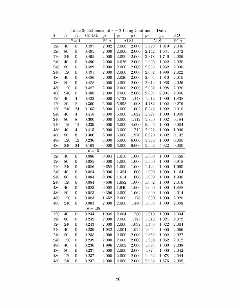
Table 3: Estimates of r = 2 Using Continuous DataT N Nc signal g2 g2 gA g2 gA AO

θ = 1 PCA ALS1 ALS PCA

120 40 0 0.497 2.002 2.006 2.000 1.998 1.010 2.040120 80 0 0.495 2.000 2.000 2.000 2.142 1.634 2.072120 240 0 0.495 2.000 2.000 2.000 3.378 1.746 2.006240 40 0 0.490 2.000 2.026 2.000 1.996 1.022 2.020240 80 0 0.489 2.000 2.000 2.000 2.006 1.932 2.030240 120 0 0.491 2.000 2.000 2.000 2.002 1.998 2.022480 40 0 0.486 2.000 2.026 2.000 2.004 1.010 2.010480 80 0 0.488 2.000 2.000 2.000 2.012 1.966 2.026480 120 0 0.487 2.000 2.000 2.000 2.002 1.998 2.020480 240 0 0.488 2.000 2.000 2.000 2.004 2.004 2.006

120 40 4 0.423 6.000 5.732 1.448 1.912 1.000 1.838120 80 8 0.300 6.000 5.998 1.008 4.782 1.002 0.276120 240 24 0.165 6.000 6.000 1.002 5.242 1.092 0.010240 40 4 0.418 6.000 6.000 1.622 1.994 1.000 1.908240 80 8 0.300 6.000 6.000 1.112 5.860 1.002 0.184240 120 12 0.239 6.000 6.000 4.600 5.966 1.000 0.004480 40 4 0.415 6.000 6.000 1.712 2.022 1.000 1.946480 80 8 0.300 6.000 6.000 1.970 5.920 1.002 0.132480 120 12 0.236 6.000 6.000 6.000 5.986 1.000 0.000480 240 24 0.162 6.000 6.000 6.000 5.992 5.922 0.000

θ = .5

120 40 0 0.086 0.004 1.010 1.000 1.000 1.000 0.488120 80 0 0.085 0.000 1.000 1.000 1.300 1.000 0.918120 240 0 0.086 0.658 1.000 1.000 1.124 1.000 1.960240 40 0 0.084 0.006 1.384 1.000 1.000 1.000 1.164240 80 0 0.084 0.096 1.614 1.000 1.000 1.000 1.930240 120 0 0.084 0.606 1.682 1.000 1.002 1.000 2.016480 40 0 0.083 0.008 1.940 1.006 1.000 1.000 1.888480 80 0 0.083 0.396 2.000 1.064 1.000 1.000 2.014480 120 0 0.083 1.452 2.000 1.178 1.000 1.000 2.020480 240 0 0.083 2.000 2.000 1.440 1.008 1.000 2.008

θ = .25

120 40 0 0.244 1.938 2.004 1.280 1.010 1.000 2.034120 80 0 0.242 2.000 2.000 1.324 1.618 1.024 2.072120 240 0 0.243 2.000 2.000 1.092 1.406 1.022 2.004240 40 0 0.239 1.982 2.004 1.924 1.064 1.000 2.066240 80 0 0.238 2.000 2.000 2.000 1.662 1.002 2.022240 120 0 0.239 2.000 2.000 2.000 1.958 1.052 2.012480 40 0 0.236 1.996 2.002 2.000 1.094 1.000 2.038480 80 0 0.237 2.000 2.000 2.000 1.874 1.000 2.042480 120 0 0.237 2.000 2.000 2.000 1.962 1.078 2.044480 240 0 0.237 2.000 2.000 2.000 2.032 1.576 2.008

26

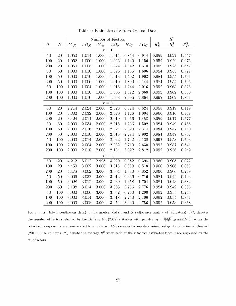
Table 4: Estimates of r from Ordinal Data

Number of Factors R2

T N ICX AOX ICx AOx ICG AOG R2X R2

x R2G

r = 1

50 20 1.050 1.014 1.000 1.014 0.854 0.914 0.959 0.927 0.557100 20 1.052 1.006 1.000 1.026 1.140 1.156 0.959 0.929 0.676200 20 1.060 1.008 1.000 1.024 1.342 1.310 0.959 0.928 0.68750 50 1.000 1.010 1.000 1.026 1.136 1.606 0.984 0.953 0.777100 50 1.000 1.010 1.000 1.018 1.502 1.962 0.984 0.955 0.791200 50 1.000 1.006 1.000 1.010 1.890 2.144 0.984 0.954 0.79650 100 1.000 1.004 1.000 1.018 1.244 2.016 0.992 0.963 0.826100 100 1.000 1.010 1.000 1.006 1.872 2.368 0.992 0.962 0.830200 100 1.000 1.016 1.000 1.058 2.006 2.864 0.992 0.962 0.831

r = 2

50 20 2.714 2.024 2.000 2.028 0.324 0.524 0.958 0.919 0.119100 20 3.302 2.032 2.000 2.020 1.126 1.004 0.960 0.916 0.368200 20 3.424 2.014 2.000 2.010 1.916 1.458 0.959 0.917 0.57750 50 2.000 2.034 2.000 2.016 1.236 1.502 0.984 0.949 0.488100 50 2.000 2.016 2.000 2.024 2.090 2.344 0.984 0.947 0.750200 50 2.000 2.010 2.000 2.016 2.784 2.902 0.984 0.947 0.79750 100 2.000 2.014 2.000 2.022 1.742 2.138 0.992 0.958 0.708100 100 2.000 2.004 2.000 2.062 2.710 2.630 0.992 0.957 0.841200 100 2.000 2.018 2.000 2.184 3.092 2.842 0.992 0.956 0.849

r = 3

50 20 4.212 3.012 2.998 3.020 0.082 0.398 0.960 0.908 0.022100 20 4.450 3.002 3.000 3.018 0.330 0.518 0.960 0.906 0.085200 20 4.478 3.002 3.000 3.004 1.040 0.852 0.960 0.906 0.24950 50 3.006 3.032 3.000 3.012 0.336 0.716 0.984 0.944 0.103100 50 3.028 3.012 3.000 3.030 1.358 1.704 0.984 0.943 0.382200 50 3.138 3.014 3.000 3.036 2.756 2.776 0.984 0.942 0.68650 100 3.000 3.006 3.000 3.032 0.760 1.290 0.992 0.955 0.243100 100 3.000 3.014 3.000 3.018 2.750 2.106 0.992 0.954 0.751200 100 3.000 3.008 3.000 3.054 3.930 2.756 0.992 0.953 0.868

For y = X (latent continuous data), x (categorical data), and G (adjacency matrix of indicators), ICy denotes

the number of factors selected by the Bai and Ng (2002) criterion with penalty g2 = N+TNT

log min(N,T ) when the

principal components are constructed from data y. AOy denotes factors determined using the criterion of Onatski

(2010). The columns R2y denote the average R2 when each of the r factors estimated from y are regressed on the

true factors.

27

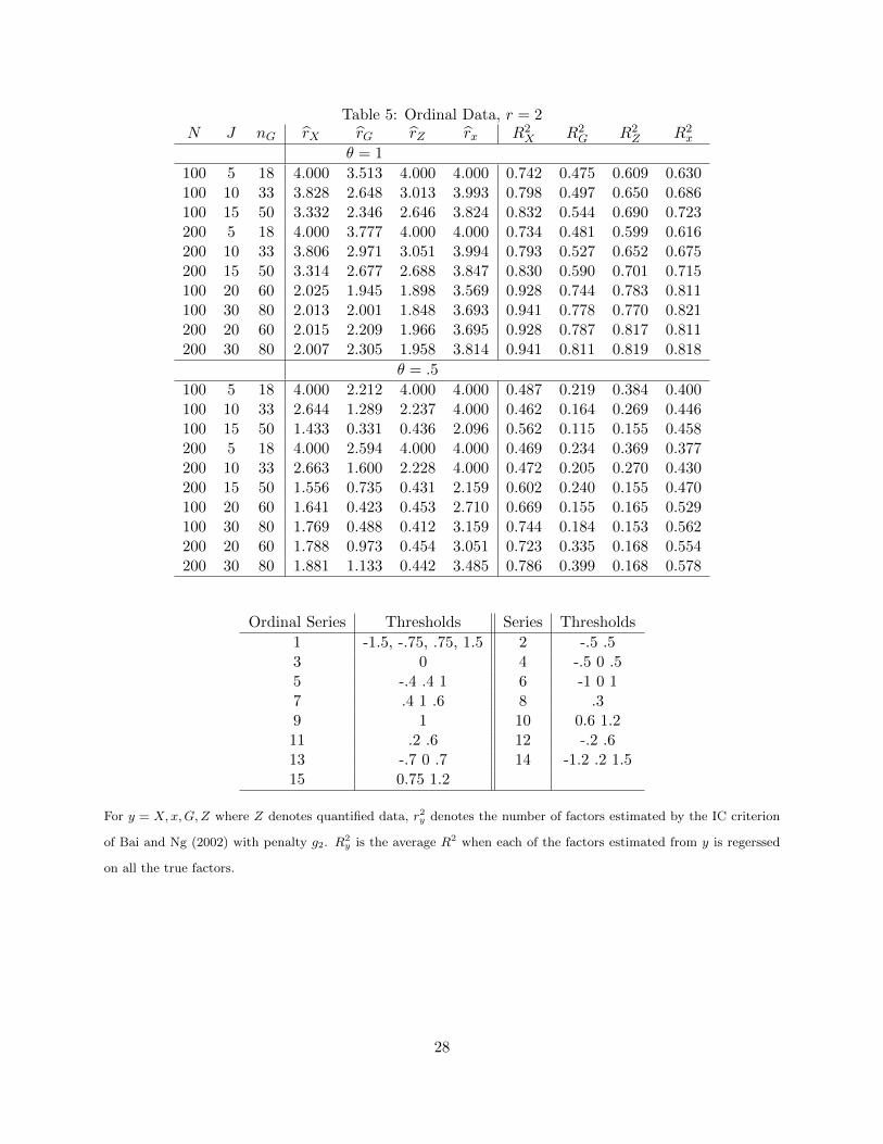
Table 5: Ordinal Data, r = 2N J nG rX rG rZ rx R2

X R2G R2

Z R2x

θ = 1

100 5 18 4.000 3.513 4.000 4.000 0.742 0.475 0.609 0.630100 10 33 3.828 2.648 3.013 3.993 0.798 0.497 0.650 0.686100 15 50 3.332 2.346 2.646 3.824 0.832 0.544 0.690 0.723200 5 18 4.000 3.777 4.000 4.000 0.734 0.481 0.599 0.616200 10 33 3.806 2.971 3.051 3.994 0.793 0.527 0.652 0.675200 15 50 3.314 2.677 2.688 3.847 0.830 0.590 0.701 0.715100 20 60 2.025 1.945 1.898 3.569 0.928 0.744 0.783 0.811100 30 80 2.013 2.001 1.848 3.693 0.941 0.778 0.770 0.821200 20 60 2.015 2.209 1.966 3.695 0.928 0.787 0.817 0.811200 30 80 2.007 2.305 1.958 3.814 0.941 0.811 0.819 0.818

θ = .5

100 5 18 4.000 2.212 4.000 4.000 0.487 0.219 0.384 0.400100 10 33 2.644 1.289 2.237 4.000 0.462 0.164 0.269 0.446100 15 50 1.433 0.331 0.436 2.096 0.562 0.115 0.155 0.458200 5 18 4.000 2.594 4.000 4.000 0.469 0.234 0.369 0.377200 10 33 2.663 1.600 2.228 4.000 0.472 0.205 0.270 0.430200 15 50 1.556 0.735 0.431 2.159 0.602 0.240 0.155 0.470100 20 60 1.641 0.423 0.453 2.710 0.669 0.155 0.165 0.529100 30 80 1.769 0.488 0.412 3.159 0.744 0.184 0.153 0.562200 20 60 1.788 0.973 0.454 3.051 0.723 0.335 0.168 0.554200 30 80 1.881 1.133 0.442 3.485 0.786 0.399 0.168 0.578

Ordinal Series Thresholds Series Thresholds

1 -1.5, -.75, .75, 1.5 2 -.5 .53 0 4 -.5 0 .55 -.4 .4 1 6 -1 0 17 .4 1 .6 8 .39 1 10 0.6 1.211 .2 .6 12 -.2 .613 -.7 0 .7 14 -1.2 .2 1.515 0.75 1.2

For y = X,x,G,Z where Z denotes quantified data, r2y denotes the number of factors estimated by the IC criterion

of Bai and Ng (2002) with penalty g2. R2y is the average R2 when each of the factors estimated from y is regerssed

on all the true factors.

28

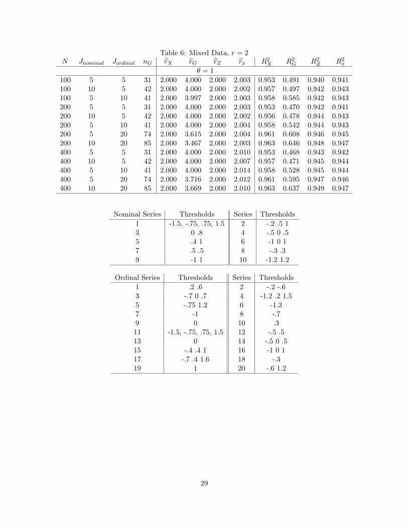
Table 6: Mixed Data, r = 2N Jnominal Jordinal nG rX rG rZ rx R2

X R2G R2

Z R2x

θ = 1

100 5 5 31 2.000 4.000 2.000 2.003 0.953 0.491 0.940 0.941100 10 5 42 2.000 4.000 2.000 2.002 0.957 0.497 0.942 0.943100 5 10 41 2.000 3.997 2.000 2.003 0.958 0.585 0.942 0.943200 5 5 31 2.000 4.000 2.000 2.003 0.953 0.470 0.942 0.941200 10 5 42 2.000 4.000 2.000 2.002 0.956 0.478 0.944 0.943200 5 10 41 2.000 4.000 2.000 2.004 0.958 0.542 0.944 0.943200 5 20 74 2.000 3.615 2.000 2.004 0.961 0.608 0.946 0.945200 10 20 85 2.000 3.467 2.000 2.003 0.963 0.646 0.948 0.947400 5 5 31 2.000 4.000 2.000 2.010 0.953 0.468 0.943 0.942400 10 5 42 2.000 4.000 2.000 2.007 0.957 0.471 0.945 0.944400 5 10 41 2.000 4.000 2.000 2.014 0.958 0.528 0.945 0.944400 5 20 74 2.000 3.716 2.000 2.012 0.961 0.595 0.947 0.946400 10 20 85 2.000 3.669 2.000 2.010 0.963 0.637 0.949 0.947

Nominal Series Thresholds Series Thresholds

1 -1.5, -.75, .75, 1.5 2 -.2 .5 13 0 .8 4 -.5 0 .55 .4 1 6 -1 0 17 .5 .5 8 -.3 .39 -1 1 10 -1.2 1.2

Ordinal Series Thresholds Series Thresholds

1 .2 .6 2 -.2 -.63 -.7 0 .7 4 -1.2 .2 1.55 -.75 1.2 6 -1.37 -1 8 -.79 0 10 .311 -1.5, -.75, .75, 1.5 12 -.5 .513 0 14 -.5 0 .515 -.4 .4 1 16 -1 0 117 -.7 .4 1.6 18 -.319 1 20 -.6 1.2

29

References

Almund, M., A. Duckworth, J. Heckman, and T. Kautz (2011): “Personality Psychologyand Economics,” NBER working paper 16822.

Anderson, T. W., and H. Rubin (1956): “Statistical Inference in Factor Analysis,” in Pro-ceedings of the Third Berkeley Symposium on Mathematical Statistics and Probability, ed. byJ. Neyman, vol. V, pp. 114–150. Berkeley: University of California Press.

Babakus, E., C. Ferguson, and K. Joreskog (1987): “The Sensitivity of Confirmatory Maxi-mum Likelihood Factor Analysis to Violations of Measurement Scale and Distributonal Assump-tions,” Journal of Marketing Research, 37(720141).

Bai, J. (2003): “Inferential Theory for Factor Models of Large Dimensions,” Econometrica, 71:1,135–172.

Bai, J., and S. Ng (2002): “Determining the Number of Factors in Approximate Factor Models,”Econometrica, 70:1, 191–221.

(2008): “Large Dimensional Factor Analysis,” Foundations and Trends in Econometrics,3:2, 89–163.

Boivin, J., and S. Ng (2006): “Are More Data Always Better for Factor Analysis,” Journal ofEconometrics, 132, 169–194.

Bollen, K. (1989): Structural Equations with Latent Variables. Wiley, New York.

Browne, M. W. (1984): “Asymptotically Distribution Free Methods in the Analysis of CovarianceStructures,” British Journal of Mathematical and Statistical Psychology, 37, 62–83.

Buja, A. (1990): “Remarks on Functional Canonical Variates: Alternating Least Squares Methodsand ACE,” Annals of Statistics, 18(3), 1032–1069.

Chamberlain, G., and M. Rothschild (1983): “Arbitrage, Factor Structure and Mean-VarianceAnalysis in Large Asset Markets,” Econometrica, 51, 1281–2304.

Cliff, N. (1966): “Orthogonal Rotation to Congruence,” Psychometrika, 31, 33–42.

Connor, G., and R. Korajzcyk (1986): “Performance Measurement with the Arbitrage PricingTheory: A New Framework for Analysis,” Journal of Financial Economics, 15, 373–394.

Conti, G., J. Heckman, H. Lopes, and R. Piatek (2012): “Constructing Economically Justi-fied Aggregates: An Application to Early Orgins of Health,” Journal of Econometrics.

Cunha, F., and J. Heckman (2008): “Formulating, Identifying and Estimating the Techology ofCognitive and Noncognitive Skill Formuation,” Journal of Human Resources, 43(4), 738–782.

De Leeuw, J. (2004): “Least Squares Optimal Scaling of Partially Observed Linear Systems,” inRecent Developments on Structural Equation Models, pp. 121–134. Kluwer Academic Publishers.

de Leeuw, J. (2005): “Monotonic Regression,” in Encyclopedia of Statistics in Behavioral Science,ed. by B. Everitt, and D. Howell, vol. 3, pp. 1260–1261. John Wiley and Sons.

Dolan, C. (1994): “Factor Analysis of Variables with 2,3,5, and 7 Response Categories: A Compar-ison of Categorical Variable Estimators Using Simulated Data,” British Journal of Mathematicaland Statistical Psychology, 46, 309–326.

Doz, C., D. Giannone, and L. Reichlin (2007): “A Quasi-Maximum Likelihood Approach forLarge Approximate Dynamic Factor Models,” ECARES working paper.

30

Filmer, D., and L. Pritchett (1998): “Estimating Wealth Effect Without Expenditure Data– Or Tears: An Application to Educational Enrollments in States of India,” Discussion Paper1994, World Bank.

Gower, J., and G. Dijksterhuis (2004): Procrustes Problems. Oxford University Press.

Harman, H., and W. Jones (1966): “Factor Analysis by Minimizing Residuals (Minres),” Psy-chometrika, 31, 563–571.

Israels, A. (1984): “Redundancy Analysis for Qualitative Variables,” Psychometrika, 49:3, 331–346.

Joreskog, K. (1994): “On the Esetimation of Polychoric Correlations and their AsymptoticCovariance Matrix,” Psychometrika, 59, 381–389.

Joreskog, K., and I. Moustki (2001): “Factor Analysis of Ordinal Variables: A Comparison ofThree Approaches,” Multivariate Behavioral Research, 36, 347–387.

Joreskog, K., and S. D. Sorbom (2006): LISREL User’s Reference GuideChicago.

Joreskog, K. G. (1970): “A Genearl Method for Analysis of Covariance Structurs,” Biometrika,57, 239–51.

(2003): “Factor Analysis by MINRES,” www.ssicentral.com/lisrel/techdocs/minres.pdf.

Keller, W., and T. Wansbeek (1983): “Multivariate Methods for Quantitative and QualitativeData,” Journal of Econometrics, 22, 91–111.

Kiers, H. (1990): “Majorization as a Tool for Optimizing a Class of Matrix Functions,” Psyhome-trika, 55(3), 417–428.

(2002): “Setting up Alternating Least Squares and Iterative Majorization Algorithms forSolving Various Matrix Optimization Problems,” Computational Statistics and Data Analysis,41, 157–170.

Kiers, H., Y. Takane, and A. Mooijaart (1993): “A Mononotically Convergent Algorithm forFACTALS,” Psychometrika, 58(4), 567–574.

Kolenikov, S., and G. Angeles (2009): “Socioeconomic Status Measurement with DiscreteProxy Variables: Is Principal Component Analysis a Reliable Answer,” Review of Income andWealth, 55(128-165).

Kruskal, J. (1964): “Nonmetric Multidimensional Scaling: A Numerical Method,” Psychome-trika, 29, 115–129.

Kruskal, J., and R. Shepard (1974): “A Nonmetric Variety of Linear Factor Analysis,” Psy-chometrika, 39, 123–157.

Lancaster, H. (1957): “Some Properties of the Bivariate Normal Distribution Considered in theform of a Contingency Table,” Biometrika, 44:1/2, 289–292.

Lawley, D. N., and A. E. Maxwell (1971): Factor Analysis in a Statistical Method. Butter-worth, London.

McDonald, R. P. (1985): Factor Analysis and Related Methods. Hilsdale, NJ: Erlbaum.

Meulman, J., and W. Heiser (2001): SPSS CategoriesSPSS Inc, 11.0 edn.

Michailidis, G., and J. de Leeuw (1998): “The Gifi System of Descriptive Multivariate Anal-ysis,” Statistical Science, 13(4), 307–336.

31

Muthen, B. (1984): “A General Structural Equation Model with Dichotomous, Ordered, Cate-gorical, and Continuous Latent Variable Indicators,” Psychometrika, 49, 115–132.

Muthen, B., and D. Kaplan (1985): “A Comparison of Some Methodologies for the FactorAnalysis of Non-normal Likert Variables,” British Journal of Mathematical and Psychology, 38,71–189.

Nevels, K. (1989): “An Improved Solution for Factals: A Nonmetric Common Factor Analysis,”Psychometrika, 54(3390343).

Olsson, U., F. Drasgow, and N. Dorans (1982): “The Polyserial Correlation Coefficient,”Psychometrika, 47:3, 337–347.

Onatski, A. (2010): “Determining the Number of Factors From Empirical Distribution of Eigen-values,” Review of Economics and Statistics, 92:4, 1004–1016.

Pearson, K. (1900): “On the Correlation of Charcters not Quantitatively Measurable,” in Mathe-matical Contributions to the Theory of Evolution: Philosophical Transactions of the Royal Societyof London, Series A, vol. 195, pp. 1–46.

Racine, J., and Q. Li (2004): “Nonparametric Estimation of Regression Functions with BothDiscrete and Continuous Data,” Journal of Econometrics, 119, 99–130.

Schonmenn, P. (1966): “A Generalized Solution of the Orthogonal Procustes Problem,” Psy-chometrika, 31(1), 1–10.

Socan, G. (2003): “The Incremental Value of Minimum Rank Factor Analysis,” Phd Thesis,University of Groningen.

Spearman, C. (1904): “General Intelligence, Objectively Determined and Measured,” AmericanJournal of Psychology, 15, 201–293.

Su, L., and A. Ullah (2009): “Functional Coefficient Estimation with Both Categorical andContinuous Data,” in Advances in Econometrics, ed. by Q. Li, and J. Racine, vol. 25, pp. 131–167. Emerald Group Publishing Limited.

Takane, Y., F. Young, and J. de Leeuw (1979): “Nonmetric Common Factor Analysis AnAlternating Least Squares Method with Optimal Scaling Features,” Behaviormetrika, 6, 45–56.

ten Berge, J. (1993): Least Squares Optimization in Multivariate Analysis. DSWO Press, Leiden.

ten Berge, J., and K. Nevels (1997): “A General Solution to Mosier’s Oblque ProcrustesProblem,” Psychometrika, 42, 593–600.

Tenenhaus, M., and F. Young (1985): “An Analysis and Synthesis of Multiple Correspon-dence Analysis, Ooptimal Scaling, Dual Scaling, Homogeneity Analysis and Other Methods forQuantifying Categorical Multivariate Data,” Psychometrika, 50(1), 91–119.

Trendafilov, N., and S. Unkel (2011): “Exploratory Factor Analysis of Data Matrices withMore Variables Than Observations,” Journal of Computational Graphical Statistics, 20, forth-coming.

Unkel, S., and N. Trendafilov (2010): “Simultaneous Parameter Estimation in ExploratoryFactor Analysis: An Expository Review,” International Statistical Review, 78:3, 363–382.

32