Louisiana State UniversityLSU Digital Commons

LSU Master's Theses Graduate School

2013

Constructing geographic areas for homicideresearch : a case study of New OrleansLawrence Keenan RobertLouisiana State University and Agricultural and Mechanical College

Follow this and additional works at: https://digitalcommons.lsu.edu/gradschool_theses

Part of the Social and Behavioral Sciences Commons

This Thesis is brought to you for free and open access by the Graduate School at LSU Digital Commons. It has been accepted for inclusion in LSUMaster's Theses by an authorized graduate school editor of LSU Digital Commons. For more information, please contact gradetd@lsu.edu.

Recommended CitationRobert, Lawrence Keenan, "Constructing geographic areas for homicide research : a case study of New Orleans" (2013). LSU Master'sTheses. 226.https://digitalcommons.lsu.edu/gradschool_theses/226

CONSTRUCTING GEOGRAPHIC AREAS FOR HOMICIDE RESEARCH:

A CASE STUDY OF NEW ORLEANS, LOUISIANA

A Thesis

Submitted to the Graduate Faculty of the

Louisiana State University and

Agricultural and Mechanical College

in partial fulfillment of the

requirements for the degree of

Master of Science

in

The Department of Geography and Anthropology

by

Lawrence Keenan Robert

B.A., Louisiana State University, 2008

May 2013

ii

For my father,

Lawrence C. Robert, Jr.

1948 - 2011

Light many lamps and gather round his bed.

Lend him your eyes, warm blood, and will to live.

Speak to him; rouse him; you may save him yet.

But death replied: ‘I choose him.’ So he went,

And there was silence in the summer night;

Silence and safety; and the veils of sleep.

iii

Acknowledgements

First, I would like to express my sincere thanks to my thesis advisor, Dr. Fahui Wang, for

his patient and thorough guidance throughout the process of researching and writing this study. I

thank my thesis committee members Dr. Michael Leitner and Dr. Lei Wang for providing a

thorough challenge for my defense and helping immensely in my creation of a polished work.

I would like to thank Dr. William Rowe, not only because with his passion for the subject

matter and intellectual rigor of instruction he convinced me to enter Geography as a profession,

but also because of his support and guidance during my time as a graduate student. I would also

like to thank Dr. Kent Mathewson, who served as my interim thesis advisor upon my entrance

into the graduate program at LSU. Thank you to Dr. Darren Purcell of the Department of

Geography and Environmental Sustainability at the University of Oklahoma for his support,

guidance, and friendship over the past few years.

I thank my friends and mentors, Jason “Tito” Sanchez, not least of all for exhorting me as

a teenager to “study your Geography”; and GySgt David Dunn, USMC, for always reminding me

to “stay strong.”

Many thanks to my fellow students and friends: Tyler Stroda, Joshua Rosby, Connor Junkin,

Kevin Oubre, Steve Beckage, Adam McLain, Garrett Wolf, Medea Gugeshashvili, Chris

Westergaard, Sofia Daraselia, Emil McClellan, 2ndLt. Noel Marcantel, USMC, Jessica

Meisinger, Ph.D., Melissa Seanard, Seth Warner, Gamze Ertuğ, Brooke Pezdirtz, Shawn

Gorman, Richard Dufreche, and Murray Melvin.

Most of all, I express my eternal love and gratitude to my mother, Mrs. Claire B. Jacobi,

and my father, the late Lawrence C. Robert, Jr., for their lifelong love, support, courage, and

sacrifice, without which I would have never succeeded.

iv

Table of Contents

Acknowledgements ........................................................................................................................ iii

Abstract .......................................................................................................................................... vi

1. Introduction ................................................................................................................................. 1

1.1 Research Motivation ............................................................................................................. 2

1.2 Research Objectives .............................................................................................................. 3

2. Literature Review........................................................................................................................ 4

2.1 Social Disorganization and Concentrated Disadvantage ...................................................... 5

2.2 The Small Population Problem ............................................................................................. 7

2.3 Regionalization Methods and REDCAP ............................................................................... 8

3. Data Sources and Processing .................................................................................................... 11

3.1 Population, Socioeconomic Data, and Concentrated Disadvantage ................................... 11

3.2 Spatial Data ......................................................................................................................... 11

3.3 Homicide Data .................................................................................................................... 12

3.4 Data Processing ................................................................................................................... 14

4. Defining the Concentrated Disadvantage Index ....................................................................... 15

5. Constructing New Geographic Areas from Census Tracts by REDCAP ................................. 21

5.1 Full-Order Average Linkage Clustering Method ................................................................ 21

5.2 Processing Parameters and Output...................................................................................... 23

6. Analysis of Spatial Distribution of Homicides ......................................................................... 27

6.1 Mean Center and Directional Distribution .......................................................................... 27

6.2 Geovisualization of Homicide Rates .................................................................................. 28

6.3 Spatial Autocorrelation of the Variables............................................................................. 31

6.4 Local Test of Spatial Autocorrelation ................................................................................. 33

7. Analysis of Association between Concentrated Disadvantage and Homicide Rate ................. 37

v

7.1 OLS Regression Analysis ................................................................................................... 37

7.2 Geographically Weighted Regression: Evaluating Spatial Non-stationarity ...................... 39

8. Conclusion ................................................................................................................................ 44

References ..................................................................................................................................... 47

Appendix: New Orleans Neighborhoods ...................................................................................... 52

Vita ................................................................................................................................................ 53

vi

Abstract

Because homicides are rare events, criminologists must often deal with the Small

Population Problem, which creates unreliable homicide rates based on arbitrarily delineated

census tracts of low population. These rates lead to violations in several assumptions required in

statistical analysis. This study proposes the Regionally Constrained Agglomerative Clustering

and Partitioning (REDCAP) method to mitigate the Modifiable Areal Unit Problem and solve the

Small Population Problem by constructing new, larger regions with sufficient minimum

populations for homicide rate calculation. This method is used for a case study of New Orleans,

Louisiana, to test the relationship between concentrated disadvantage and homicide. Ordinary

Least Squares and Geographically Weighted Regressions are conducted with the data both before

and after the REDCAP operation. Results for the standard census tract layer show a weak and

insignificant relationship between concentrated disadvantage and homicide because of extremely

unreliable rate estimates. After the REDCAP operation, variables show a more normal

distribution and reduced variability; moreover, regression results confirm a strong and positive

relationship between concentrated disadvantage and homicide. This study shows viability for

REDCAP as a regionalization method for further studies on violent crime, namely its ability to

provide more stable data for improved reliability in crime rate calculations. Additionally, this

study provides implications for public policy, specifically social cohesion and efficacy policies,

including community-oriented policing.

.

1

1. Introduction

“…New York City, with more than 20 times the population of New Orleans, had 536 murders

last year. If New York had New Orleans's homicide rate, more than 4,000 people would have

been murdered there last year, about 11 every day.” (McCollam 2011)

After the world’s 20 deadliest cities, all in Latin America, plagued by drug- and gang-

related violence, New Orleans is the 21st deadliest city in the world and by far the deadliest city

in the United States. In many cities, gang and drug violence is the dominant factor in driving up

the violent crime and homicide rates; however, the New Orleans Police Department and many

researchers believe that the problem is less linked to gang activity or narcotics than in other

cities, although these factors likely contribute not insignificantly (McCollam 2011). Recently,

the City of New Orleans including the New Orleans Police Department is increasingly aware that

building trust between residents and the police is the key to reducing the murder rate (Elliott

2012, Maggi 2012, Newkirk 2012); however, the new policies have not been implemented long

enough to ascertain whether they have had a significant effect on the number of homicides.

Sociologists have long tried to determine the causes of violence in urban areas. Drawing

from the significant work in that academic discipline, this study intends to show that the link of

the homicide rate to the structural characteristics of neighborhoods, namely the high

concentration of disadvantage in certain neighborhoods in New Orleans. This extreme socio-

economic disadvantage leads to a high level of social disorganization, with which researchers

have long shown an association with high crime rates. Social disorganization and concentrated

disadvantage are indicated by many socio-demographic factors including racial segregation,

single parenthood, unemployment, and poverty. These indicators have been linked to lower

levels of physical health, increased levels of depression, lower neighborhood cohesion, and

lower neighborhood trust, all of which form the pathway to an intractable cycle of violent crime

2

and homicide in particular. This study will demonstrate the relationship between the

concentrated disadvantage and elevated homicide rates in New Orleans, Louisiana.

1.1 Research Motivation

The Port of New Orleans is one of the largest in the United States due to its strategic

position at the mouth of the Mississippi River and near the oil production facilities in the Gulf of

Mexico. The city is a major tourist destination and relies on tourism revenue to drive its

economy. The annual Mardi Gras festival draws so many people in a short period of time that

the total amount of garbage collected becomes a reliable metric of its economic impact. The city

has hosted the National Football League Super Bowl ten times since 1970 – more than any other

city except Miami. In 2012, tourism to the city had a record total economic impact of $5.46

billion from 8.75 million people; moreover, the tourism industry employs more than 70,000

people, making it the metropolitan area’s biggest employer (Krupa 2012; NOCVB 2012).

Unfortunately, the consistently triple-digit homicide counts and other crime incidence

have been the cause of a major concern for potential visitors to the city. On any given day of the

week, a casual glance at the city’s long-time newspaper, The Times-Picayune, reveals tales of

crime committed just hours before publishing. City business, political, and cultural leaders have

lamented a common belief that crimes in New Orleans are geographically widespread rather than

geographically concentrated. This misconception may deter many potential tourists from visiting

the city in fear of widespread crime. In fact, most crimes involving tourists are petty thefts and

do not correspond to areas of high crime rates in the city. Examining the geographic

concentration of crime, including its most severe type, homicide, and its association with

socioeconomic disadvantage has important implication in public policy. One major shift in

criminal theories as well as policing strategies since the 1980s is from “offender-based” to

3

“place-based” approaches (Wang 2012). In this sense, this study lends support to targeted (hot-

spot) policing and community-oriented policing, which have proven to be effective in various

jurisdictions in the U.S.

1.2 Research Objectives

The objectives of this study are twofold. The first is to test the relationship between the

concentration of socioeconomic disadvantage and homicides in Orleans Parish, Louisiana using

geo-statistical analysis techniques. The second objective of this study is to construct larger

geographic areas from census tracts by a GIS-based automatic regionalization technique to

obtain reliable homicide rates, which permit meaningful mapping and statistical analysis.

Homicide researchers have frequently run into problems regarding the method of delineation of

census tracts: small base populations in some tracts used in calculating homicide rates produce

results that are sensitive to errors in the data and may violate the assumption of heterogeneity of

error variance in regression analysis. The study sets forth two hypotheses. The first hypothesis

is that there is a positive and significant relationship between concentrated socioeconomic

disadvantage and the homicide rate in the study area. The second hypothesis is that the

aforementioned problems are mitigated by the new analysis areas derived from the

regionalization method.

4

2. Literature Review

The hypotheses of this study require the discussion of two bodies of theoretical literature

to understand what is being tested. The first hypothesis involves the exploration a large body of

thought in sociological research beginning the 1940s which examines the causes of crime,

specifically socioeconomic disadvantage and its relation to the structure of communities. This

research begins with a theory known as social disorganization and leads to a set of more concrete

indicators known as concentrated disadvantage. The second hypothesis deals with theoretical

and applied research in geography which discusses methods to solve statistical issues that arrive

from a fundamental problem in quantitative geographical research. The methods discussed

involve approaches of mitigating the small population problem including creating new areas

from smaller ones, so-called “regionalization” methods. Both of these bodies of literature are

briefly introduced here and then discussed in detail.

Literature theoretically supporting the first hypothesis begins with the sociologists Shaw

and McKay (1942), who pioneered the idea of “social disorganization,” a term referring to the

link between poverty and other factors and the breakdown of societal organization. As the

organization decreases, crime rates increase. The sociological literature shows that a set of

factors called “concentrated disadvantage” best indicates the level of disorganization within a

particular community. This is explained in depth in section 2.1. The theoretical basis of the

second hypothesis draws from the substantial research in quantitative geography and

criminology. Arbitrarily-defined areal units create error and bias in statistical observations as

discussed in section 2.2. This study seeks to mitigate the issue by using a method for automatic

regionalization of the census tracts in the study area as discussed in section 2.3.

5

2.1 Social Disorganization and Concentrated Disadvantage

Social disorganization can be defined as “the inability of a community structure to realize

common values of its residents and maintain effective social controls” (Sampson and Groves

1989, 777). Social disorganization has long been used to link crime incidence with disadvantage

in the population. This theory (Shaw & McKay 1942) was developed to show that certain

factors, such as ethnic heterogeneity and poverty, lead to the breakdown of organization within

the community and, therefore, increases in crime within that community (Sampson and Groves

1989). The opposite of this would be social organization or collective efficacy, which is defined

as willingness of neighbors “to intervene on the behalf of the common good” and is thought to

reduce neighborhood violence (Sampson et al. 1997, 918). Where disorder is perceived in the

community and the built environment, indicators of social disorganization are increased. Higher

levels of social disorganization are a source of neighborhood violence because it lowers the

degree of informal social controls that would otherwise mitigate delinquent behavior (Hoffman

2003, Sampson et al 1997). Disorganized communities frequently show levels of trust, cohesion,

mental health, and physical health; and thus increased crime rates, including those of violent

crime (Bellair 1997, Hoffman 2003, Kawachi et al. 1999, Sampson and Groves 1989, Sampson

et al. 1997, Swaroop and Morenoff 2006, Taylor 1996, Taylor and Covington 1993).

Research has linked social disorganization and concentrated levels of disadvantage (Hipp

2010, Sampson and Groves 1989, Sampson et al 1997). Concentrated disadvantage is a term for

a number of structural factors within a community or neighborhood that lead to social

disorganization. Sampson et al. (1999, 657) argued that “neighborhood disadvantage should be

expanded beyond the simple notion of rates of poverty.” There is a significant body research

6

which examines indicators of concentrated disadvantage. For instance, scholars have discussed

the ecological concentration of poverty in black neighborhoods.

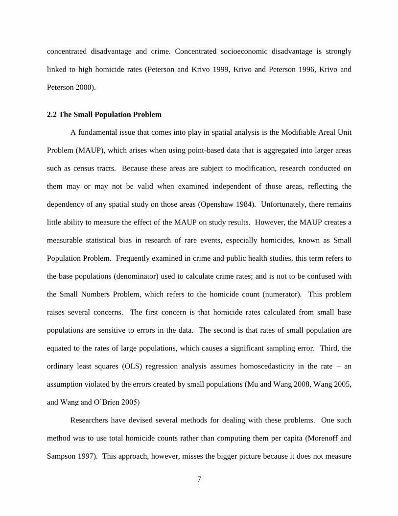
Highly discriminatory broker-side housing market practices effectively segregate white

and black communities, thus limiting the latter to disadvantaged neighborhoods; this has an

effect on black homicide rates without a corresponding effect for whites. High unemployment

has been an observed indicator of concentrated disadvantage: segregation has the effect of

lowering employment, which can increase the homicide rate (Krivo et a. 1998, Lee 2000, and

Peterson and Krivo 1999). In addition to constrained choices of residence, lower employment,

and poverty, single-parent families have been shown to be a significant indicator of concentrated

disadvantage. The combination of poverty and single-parent households has been shown to be

deleterious to social organization; moreover, concentrated disadvantage has been shown to

increase out-of-wedlock births and single parentage as a result (De Coster et al. 2006, South

2001). This, in turn, can raise rates of depression in adults because of the stress of the perception

of the disorder at the neighborhood level (Ross 2000).1 An observed result of this ecological

environment is an increase in individuals receiving public assistance (De Coster et al. 2006,

Kubrin and Weitzer 2003).

Sampson et al. (1997) point to the level of social control and trust in advantaged

neighborhoods as a predictor of lower violent crime rates. There are frequently lower levels of

trust among residents in disadvantaged neighborhoods (Ross et al. 2001). As social control

breaks down due to concentrated disadvantage, the frequency of informal conflict resolution

increases. Homicide (and retaliatory homicide) increase with levels of concentrated

disadvantage (Kubrin and Weitzer 2003). Hipp (2010) noted a reciprocal relationship between

1 A poor-quality built environment has also been linked to depression (Galea et al. 2005) and crime (Wei et al.

2005).

7

concentrated disadvantage and crime. Concentrated socioeconomic disadvantage is strongly

linked to high homicide rates (Peterson and Krivo 1999, Krivo and Peterson 1996, Krivo and

Peterson 2000).

2.2 The Small Population Problem

A fundamental issue that comes into play in spatial analysis is the Modifiable Areal Unit

Problem (MAUP), which arises when using point-based data that is aggregated into larger areas

such as census tracts. Because these areas are subject to modification, research conducted on

them may or may not be valid when examined independent of those areas, reflecting the

dependency of any spatial study on those areas (Openshaw 1984). Unfortunately, there remains

little ability to measure the effect of the MAUP on study results. However, the MAUP creates a

measurable statistical bias in research of rare events, especially homicides, known as Small

Population Problem. Frequently examined in crime and public health studies, this term refers to

the base populations (denominator) used to calculate crime rates; and is not to be confused with

the Small Numbers Problem, which refers to the homicide count (numerator). This problem

raises several concerns. The first concern is that homicide rates calculated from small base

populations are sensitive to errors in the data. The second is that rates of small population are

equated to the rates of large populations, which causes a significant sampling error. Third, the

ordinary least squares (OLS) regression analysis assumes homoscedasticity in the rate – an

assumption violated by the errors created by small populations (Mu and Wang 2008, Wang 2005,

and Wang and O’Brien 2005)

Researchers have devised several methods for dealing with these problems. One such

method was to use total homicide counts rather than computing them per capita (Morenoff and

Sampson 1997). This approach, however, misses the bigger picture because it does not measure

8

the number of homicides relative to the population (homicides per capita). Another method is

removing small population samples (Harrel and Gouvis 1994, Morenoff and Sampson 1997).

This avoids the problem of unreliable rates based on small populations but removes data that

could possibly be critical to the analysis. Messner et al. (1999), and studies reviewed by Land et

al. (1990) attempt to fix the problem by aggregating the data to a large geographical area, such as

entire cities or states, or over longer time periods (see also Wang and Arnold 2008) – both of

which are likely to reduce the resolution and accuracy of the analysis. Yet a fourth method for

resolving the issue uses Poisson regressions to account for error variances in the variables (Land

et al. 1996; Osgood 2000, Osgood & Chambers 2000). The final method discussed here is

regionalization, that is to construct “areas with sufficiently large base populations” (Wang and

O’Brien 2005), a method employed by Haining et al. (1994), Haining et al. (1998), Black et al.

(1996), Sampson et al. (1997), Mu and Wang (2008), and Wang et al. (2012). This allows

reliable rates to be calculated by setting a minimum threshold population, which provides for

more accurate statistical analysis, particularly regressions. The next section is devoted to further

discussion of the regionalization method as it is employed in this study.

2.3 Regionalization Methods and REDCAP

Spatial analysts have several methods available for the construction of new geographical

areas. Two similar methods use proximity as the main determinant of constructed regions.

Black et al. (1996) and Haining et al. (1994) employed the ISD, or Sheffield method (named after

the region in the study), which simply adds neighboring tracts the minimum threshold population

is reached. Lam and Liu (1996) utilized the spatial order method to create regions of 50

HIV/AIDS cases per region and required roughly equal geographical size per region. This

method makes use of space-filling curves to determine proximity of neighboring regions. Wang

9

and O’Brien (2005) employed both the ISD and the spatial order methods to construct regions of

similar environmental classifications with minimum thresholds to analyze the “Herding Culture

of Honor” hypothesis of homicide. Wang (2005) and Mu and Wang (2008) developed the space-

scale method of regionalization, used by Wang (2005) in his study of Chicago homicide. This

method is drawn from a smoothing process used in imagery interpretation and emphasizes

homogeneity of attributes.2 Haining et al. (1998) regionalized based on the Exploratory Spatial

Data Analysis (ESDA) methods in the SAGE software package, which is a set of techniques that

allows users to choose the use of local or global statistics and how proximity is defined.

In their study of cancer rates in Illinois, Wang et al. (2012) used the REDCAP method

which this study proposes as an effective means to mitigate the Small Population Problem in its

case study of New Orleans, LA. Guo (2008) developed Regionalization with Dynamically

Constrained Agglomerative Clustering and Partitioning (REDCAP). Much like the space-scale

method, REDCAP groups areas by homogeneity while retaining adjacency. There are two

processes in the REDCAP method: first, the operation clusters regions based into a contiguity-

constrained hierarchy; and second, the operation partitions that tree from the top down. There

are four algorithms for clustering: SLK, ALK, CLK, and Ward; and two algorithms for

partitioning: first-order and full-order (Guo 2008, Guo and Wang 2011). This method is

discussed in detail in Chapter 5.

This chapter discussed the literature that composes the theoretical bases of the study’s

hypotheses. The first hypothesis concerning concentrated disadvantage and homicide requires

that several variables, including homicide rates and indicators of socioeconomic disadvantage, be

operationalized for a quantitative study. The second hypothesis concerning the mitigation of the

Small Population Problem requires acquisition and regionalization of study area data. These data

2 Discussed at length in Wang (2005) and Guo and Wang (2011).

10

and methods are discussed in Chapter 3, which pertains to the data sources; in Chapter 4, which

pertains to the indicators of concentrated disadvantage; and in Chapter 5, which pertains to the

regionalization of the study area. With these arguments and methods, the study will contribute

both an explanation of homicide in New Orleans, Louisiana and empirical support for the use of

REDCAP regionalization as an effective tool in criminological research.

11

3. Data Sources and Processing

The previous chapter stated that this study requires several sources of data. First is the

census data (section 3.1), which is provided by the United States Census Bureau. Second is the

spatial data (section 3.2), which contains both the number and geolocation of the incidents.

Third is the population and socioeconomic data taken from the 2010 Census (section 3.3). This

data is particularly useful because it is data collected from the most recent Census. The

processing (section 3.4) of these data is also discussed below.

3.1 Population, Socioeconomic Data, and Concentrated Disadvantage

Data on population and selected socioeconomic characteristics were taken from the 2010

Census American Community Survey (ACS) via the American FactFinder website

(http://factfinder2.census.gov/faces/nav/jsf/pages/index.xhtml). In years between censuses, the

ACS provides estimated data with a margin of error; however, in Census years, the ACS

provides the exact counts acquired without a margin of error. The specific socioeconomic

indicators taken from the Census data are discussed further in Chapter 4.

3.2 Spatial Data

The spatial layers used for this study were acquired from the United States Census

Bureau’s TIGER/Line (Topologically Integrated Geographic Encoding and Referencing)

Shapefile products. The extent of the study area is the boundaries of Orleans Parish, Louisiana,

rather than the entire metropolitan statistical area. The city of New Orleans and Orleans Parish

are coterminous. The extent was chosen based on the fact that the homicide data is for Orleans

Parish only (see section 3.3). Layers for census tracts and area water were used for mapping,

though area water is purely used for reference and not analytical purposes. All layers were

12

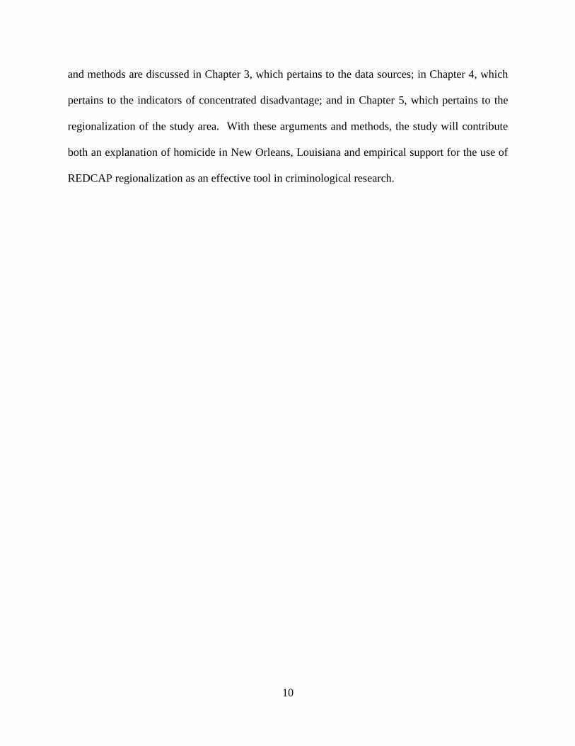
added into the GIS and projected into Universal Transverse Mercator. The homicide point layer

was joined to the tract layer based on common spatial location. Census tracts 9801 (swamp) and

9900 (Lake Ponchartrain) were excluded from the study area because they are both uninhabited

and contain no homicides.

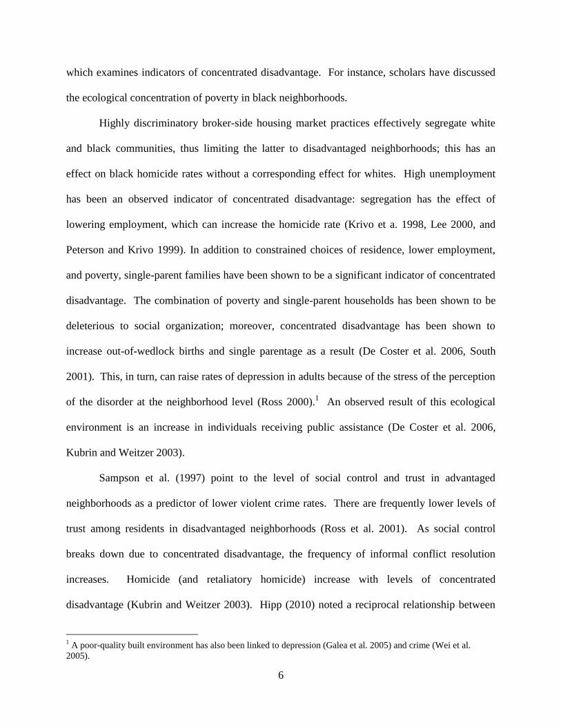
Figure 3.1: Orleans Parish, Louisiana

3.3 Homicide Data

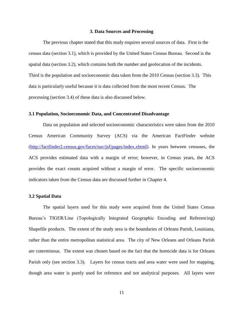
A sample (n=708) homicide events occurring between January 3, 2008 and March 24,

2012 in Orleans Parish, Louisiana was compiled and geocoded by The Times-Picayune

newspaper, which placed the data online for public use. Data is victim-side only and includes

date, age, address, neighborhood, time, and manner of death. Multiple homicides occurring at

the same location events, which constituted 6.4% of the sample, were aggregated into single

13

events by the newspaper. Each event included in the data set was geocoded from the address of

the crime by the Google Maps GIS. The data set also includes a URL to the newspaper report

concerning each homicide. The data was processed into an ArcGIS Point Layer shapefile,

projected to the Universal Transverse Mercator projection and added into the GIS.

The dataset may be found at

https://www.google.com/fusiontables/DataSource?docid=182KOD7FP6GMNKeZw6mTaAIiMZ

gQ1npuiRyBK1kQ

Figure 3.2: The Study Area and Homicide Incidents

14

3.4 Data Processing

This thesis primarily uses the ArcGIS 10 for Desktop Geographical Information System

(GIS) for the storing, display, and analysis of geographical data. The software, which is

produced by ESRI, enables complex geographical statistical analysis of the data. More

information on this package can be found at http://www.esri.com/software/arcgis. The java-

based software package REDCAP (Regionalization with Dynamically Constrained Agglomerative

Clustering & Partitioning) is used to further process the data as required for further analysis. This

package is available free of charge at http://www.spatialdatamining.org/software/redcap.

Regression analysis was performed via the Data Analysis package contained in the Microsoft

Excel 2010 spreadsheet software.

15

4. Defining the Concentrated Disadvantage Index

There are a number of indicators of concentrated disadvantage as discussed in the

literature review (Chapter 2). The experimental design process included an assessment of how to

operationalize these indicators as variables in the study. To integrate these variables, a

Concentrated Disadvantage Index (CDI) was created using the mean of the standard scores of

each variable. Here the method is discussed in detail.

The method for creation of the CDI is drawn from and Swaroop and Morenoff (1996) and

Benson and Fox (2004). The latter explained that “the crime-related effects of community

disadvantage are not linear…rather, they tend to only appear in the most distressed

neighborhoods as concentration effects” (Benson and Fox 2004, II-3-5). In their studies, the

researchers selected variables that are indicators of concentrated disadvantage and extracted

them from the ACS data. Those variables are percentage of people below the poverty line,

percentage of African-American individuals, percentage of single-parent households, percentage

on public assistance (both welfare and food stamps), and the unemployment rate. The authors

then took the mean of the standard scores of each variable (Benson and Fox, 2004).

There are a couple of limitations to this method. First, no factor analysis was conducted

on each variable to determine if weighting is appropriate. This was deemed not necessary in the

experimental design as to follow the model as closely as possible. Second, some of the variables

could have significant overlap. For instance, a large portion of individuals receiving public

assistance are also unemployed and living in segregated areas. This might require exploratory

regression analysis with multiple variables; however, given the dual hypotheses set forth in the

research objectives, a multivariate regression analysis was deemed unnecessary and beyond the

scope of this study. Finally, the population data itself may have limits as it is only the count of

16

individuals in residence. Andresen (2011) argues that the ambient population may be a better

indicator of violent crime victimization than census population counts; this may be even more

true when routine activity theory – the fact that offender and victim must be in the same place –

is considered (Cohen and Felson 1979) however, given the difficulty of obtaining the data to

calculate the population, this measure was foregone in the experimental design.

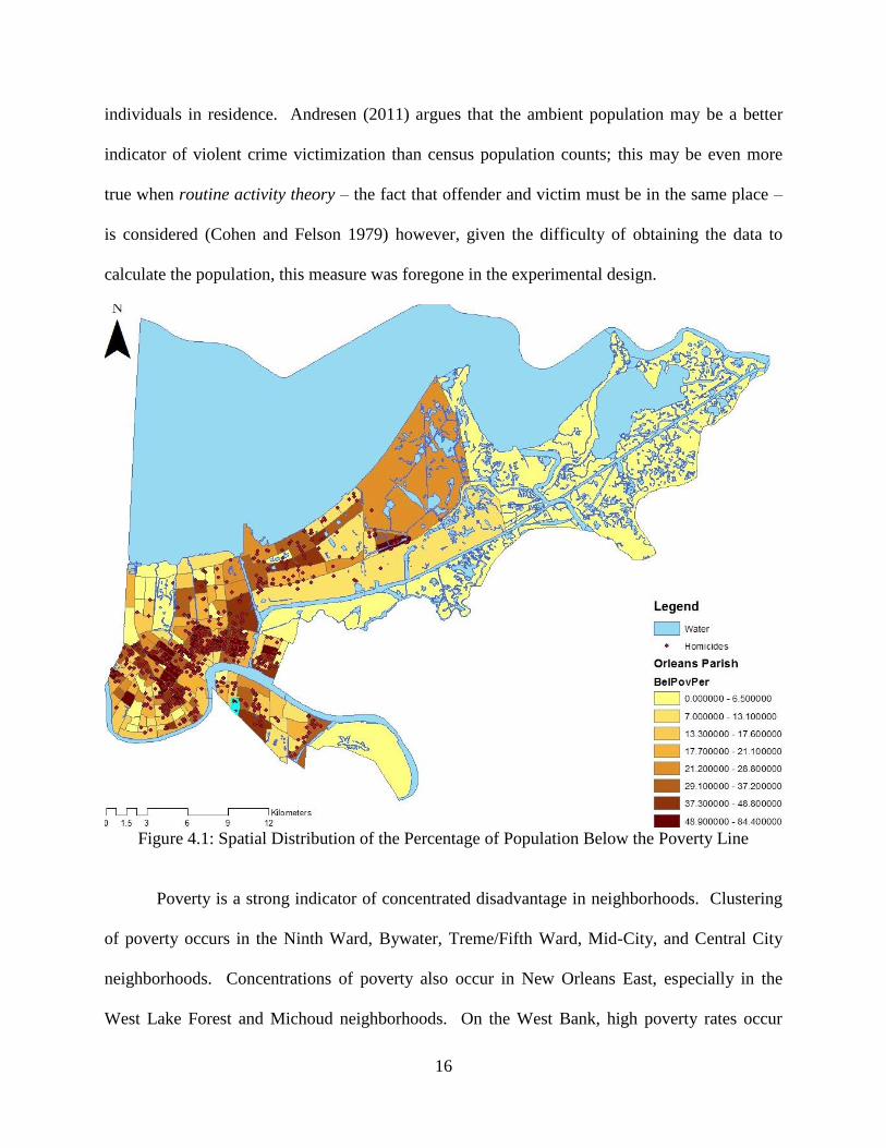
Figure 4.1: Spatial Distribution of the Percentage of Population Below the Poverty Line

Poverty is a strong indicator of concentrated disadvantage in neighborhoods. Clustering

of poverty occurs in the Ninth Ward, Bywater, Treme/Fifth Ward, Mid-City, and Central City

neighborhoods. Concentrations of poverty also occur in New Orleans East, especially in the

West Lake Forest and Michoud neighborhoods. On the West Bank, high poverty rates occur

17

south and southwest of Algiers and southeast of Old Aurora. Note the observed clustering of

homicides among more impoverished areas (Figure 4.1).

Another indicator of concentrated disadvantage discussed in the literature review that is

closely related to poverty is the unemployment rate. The spatial distribution of the

unemployment rate is somewhat similar to that of the percentage below the poverty line;

however, census tracts that have high levels of poverty may not have equally as high

unemployment rates and vice-versa. Because there is not a one-to-one relationship between the

two variables, using both of these as indicators of disadvantage is necessary and justified. Figure

4.2 displays the spatial distribution of the unemployment rate within Orleans Parish.

Figure 4.2: Spatial Distribution of the Unemployment Rate

18

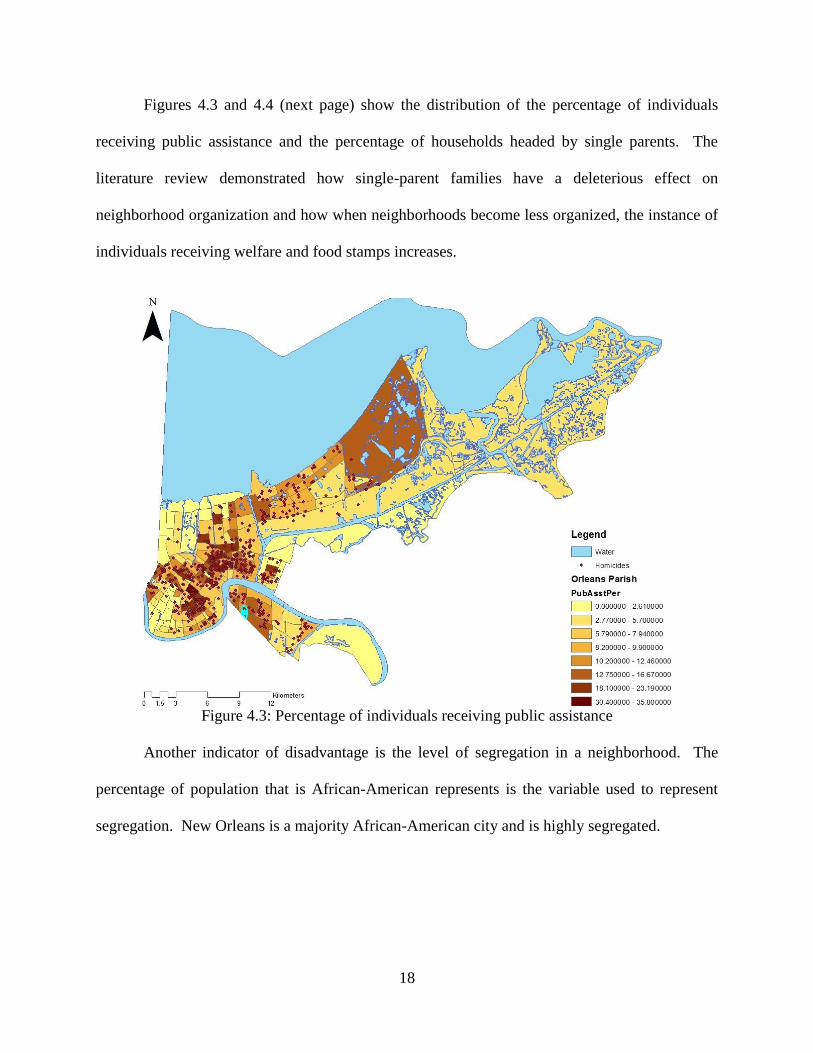
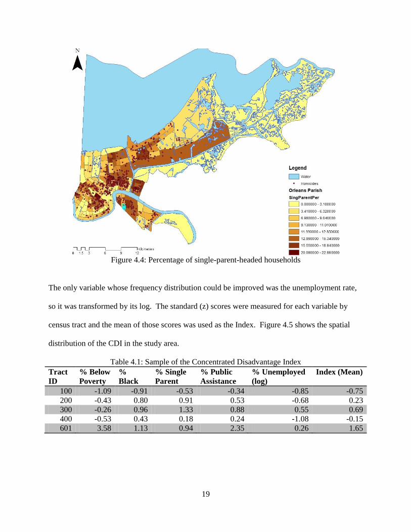
Figures 4.3 and 4.4 (next page) show the distribution of the percentage of individuals

receiving public assistance and the percentage of households headed by single parents. The

literature review demonstrated how single-parent families have a deleterious effect on

neighborhood organization and how when neighborhoods become less organized, the instance of

individuals receiving welfare and food stamps increases.

Figure 4.3: Percentage of individuals receiving public assistance

Another indicator of disadvantage is the level of segregation in a neighborhood. The

percentage of population that is African-American represents is the variable used to represent

segregation. New Orleans is a majority African-American city and is highly segregated.

19

Figure 4.4: Percentage of single-parent-headed households

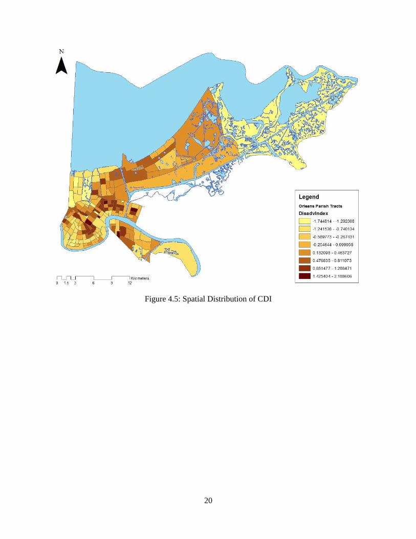
The only variable whose frequency distribution could be improved was the unemployment rate,

so it was transformed by its log. The standard (z) scores were measured for each variable by

census tract and the mean of those scores was used as the Index. Figure 4.5 shows the spatial

distribution of the CDI in the study area.

Table 4.1: Sample of the Concentrated Disadvantage Index

Tract

ID

% Below

Poverty

%

Black

% Single

Parent

% Public

Assistance

% Unemployed

(log)

Index (Mean)

100 -1.09 -0.91 -0.53 -0.34 -0.85 -0.75

200 -0.43 0.80 0.91 0.53 -0.68 0.23

300 -0.26 0.96 1.33 0.88 0.55 0.69

400 -0.53 0.43 0.18 0.24 -1.08 -0.15

601 3.58 1.13 0.94 2.35 0.26 1.65

20

Figure 4.5: Spatial Distribution of CDI

21

5. Constructing New Geographic Areas from Census Tracts by REDCAP

The practical need and theoretical basis for regionalization was established in the

literature review (Chapter 2). Here the REDCAP regionalization method is examined as it

pertains to the study area. REDCAP regionalization is actually a set of several different

methods. First, the particular method chosen in the experimental design process is discussed.

Then, the outputs of the process are visualized and displayed for comparison purposes.

5.1 Full-Order Average Linkage Clustering Method

The small populations created by the default delineation of census tracts in Orleans

Parish provide for extremely unreliable homicide rate observations. REDCAP allows

researchers to aggregate geographical units of a minimum threshold population and a desired

measure of homogeneity. This allows observation of patterns that may be confounded by the

heterogeneity of variables in the data set (Guo 2008, Guo and Wang 2011). RECAP requires the

construction of a contiguity matrix of the spatial layer based on either Rook or Queen contiguity.

Both the shapefile of the Orleans Parish census tract layer and its contiguity matrix are loaded

into the REDCAP application. In this case, the desired measure of homogeneity is the CDI.

There are several methods of regionalization available in the software, but in this case the Full-

Order Average Linkage Cluster (ALK) method was sufficient to regionalize based on a single

variable. A discussion of the Full-Order ALK operation follows below.3

Guo (2008) defines first-order contiguity as two neighbors that share an edge. The first

step in the REDCAP operation is to create a contiguity matrix of regions in the input data (in this

case, rook contiguity is sufficient for this operation, and is faster than queen contiguity). A

spatially contiguous hierarchy is one that is connected by first-order edges; clusters are spatially

3 For an exhaustive discussion of the REDCAP method, see Guo (2008) and Guo and Wang (2011).

22

contiguous if they consist of two hierarchies that share a first-order edge. These edges are

removed in the beginning of the regionalization process, as opposed to the full-order operation,

where the edge removal process is iterative, and edges are considered throughout the entire

operation (Guo 2008).

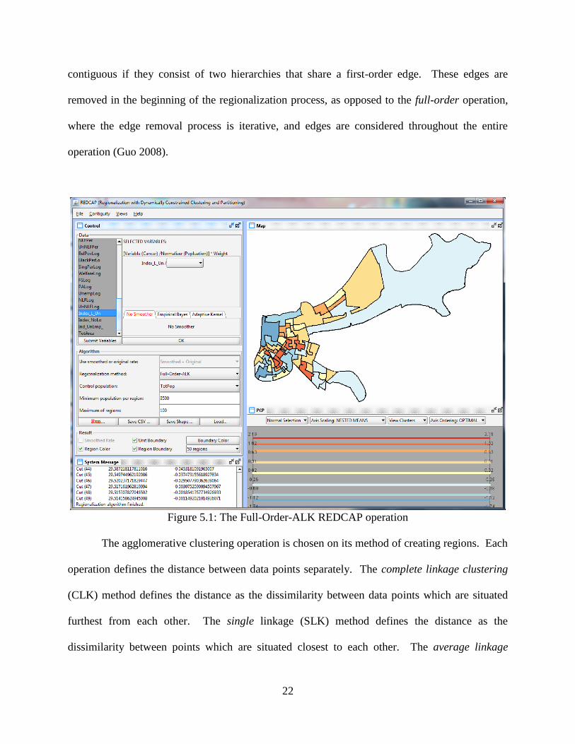
Figure 5.1: The Full-Order-ALK REDCAP operation

The agglomerative clustering operation is chosen on its method of creating regions. Each

operation defines the distance between data points separately. The complete linkage clustering

(CLK) method defines the distance as the dissimilarity between data points which are situated

furthest from each other. The single linkage (SLK) method defines the distance as the

dissimilarity between points which are situated closest to each other. The average linkage

23

clustering (ALK) is a good compromise between the two, as it defines the distance as the

average of the dissimilarity of all data points on an intra-cluster basis. The ALK method is

defined as

( )

| || |∑ ∑ (1)

Where | | and | | are the number of data points in clusters L and M, and are data

points, and is the dissimilarity. While this operation is taking place, REDCAP takes the

measure of heterogeneity and the gain in homogeneity of the regions to optimize the objective

function of construction homogenous regions as defined in Guo (2008).

5.2 Processing Parameters and Output

A natural consequence of constructing new regions from old ones is that the total number

of regions is reduced. When conducting the REDCAP operation, there was careful consideration

of the need to balance a significant reduction of the homicide rate while preventing too few

regions from existing. Too few regions would obfuscate the statistical analysis by lowering the

resolution of the study, while having too much variability in the homicide rate would defeat the

purpose of the operation. In particular, a low number of regions creates problems for

Geographically Weighted Regression by having to few neighbors to evaluate local correlations.

Trial-and-error runs of the REDCAP software determined that a fair minimum threshold

population per aggregated region is 3500, as the standard deviation was sufficiently reduced for

reliable observations in the homicide rate (Table 5.1). The maximum number of regions was

specified to 100; however, 50 regions were produced by the Full-Order-ALK algorithm at the

specified threshold (Figure 5.2). This number is on the low side of desired regions for a GWR

but is within the acceptable limit to produce accurate results. Lower threshold populations

24

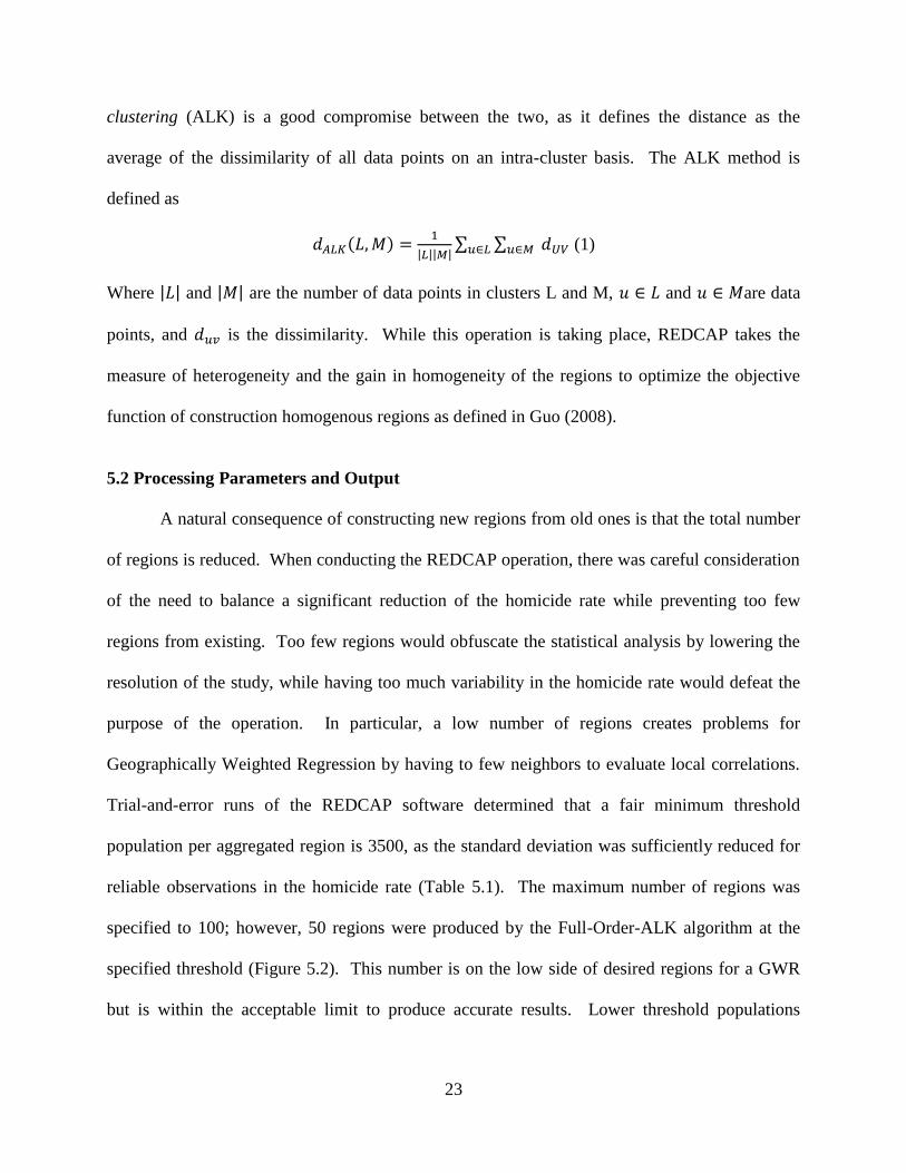
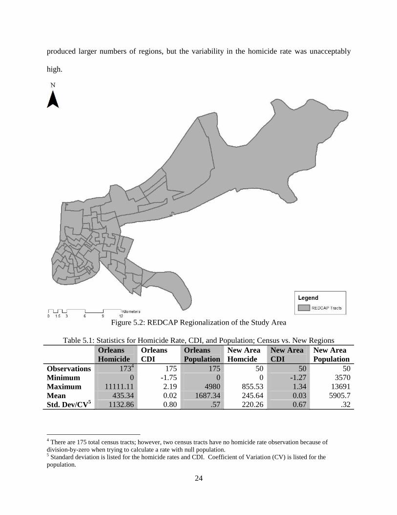
produced larger numbers of regions, but the variability in the homicide rate was unacceptably

high.

Figure 5.2: REDCAP Regionalization of the Study Area

Table 5.1: Statistics for Homicide Rate, CDI, and Population; Census vs. New Regions

Orleans

Homicide

Orleans

CDI

Orleans

Population

New Area

Homcide

New Area

CDI

New Area

Population

Observations 1734 175 175 50 50 50

Minimum 0 -1.75 0 0 -1.27 3570

Maximum 11111.11 2.19 4980 855.53 1.34 13691

Mean 435.34 0.02 1687.34 245.64 0.03 5905.7

Std. Dev/CV5 1132.86 0.80 .57 220.26 0.67 .32

4 There are 175 total census tracts; however, two census tracts have no homicide rate observation because of

division-by-zero when trying to calculate a rate with null population. 5 Standard deviation is listed for the homicide rates and CDI. Coefficient of Variation (CV) is listed for the

population.

25

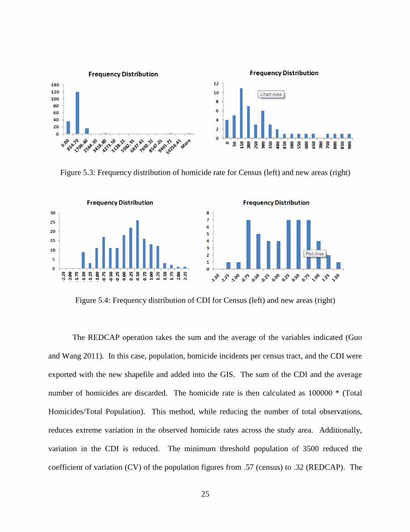
Figure 5.3: Frequency distribution of homicide rate for Census (left) and new areas (right)

Figure 5.4: Frequency distribution of CDI for Census (left) and new areas (right)

The REDCAP operation takes the sum and the average of the variables indicated (Guo

and Wang 2011). In this case, population, homicide incidents per census tract, and the CDI were

exported with the new shapefile and added into the GIS. The sum of the CDI and the average

number of homicides are discarded. The homicide rate is then calculated as 100000 * (Total

Homicides/Total Population). This method, while reducing the number of total observations,

reduces extreme variation in the observed homicide rates across the study area. Additionally,

variation in the CDI is reduced. The minimum threshold population of 3500 reduced the

coefficient of variation (CV) of the population figures from .57 (census) to .32 (REDCAP). The

26

minimum population actually achieved was extremely close to the specified input setting (Table

5.1, Figure 5.3, Figure 5.4). The next section will discuss the spatial variations in homicide rates

as they appear in the census tract layer and in the newly-created REDCAP layer.

27

6. Analysis of Spatial Distribution of Homicides

This study employed several powerful tools for geovisualization and descriptive analysis.

First the mean center and direction distribution of the homicide rates was plotted. Then an

interpolated surface trend was generated to compare homicide rates between regions of the study

area. This surface trend was generated for both the Census layer and the REDCAP layer to show

the reduction in variability. Finally, two tests of spatial autocorrelation of the variables are

conducted to ensure that the analysis in Chapter 7 does not violate any statistical assumptions.

6.1 Mean Center and Directional Distribution

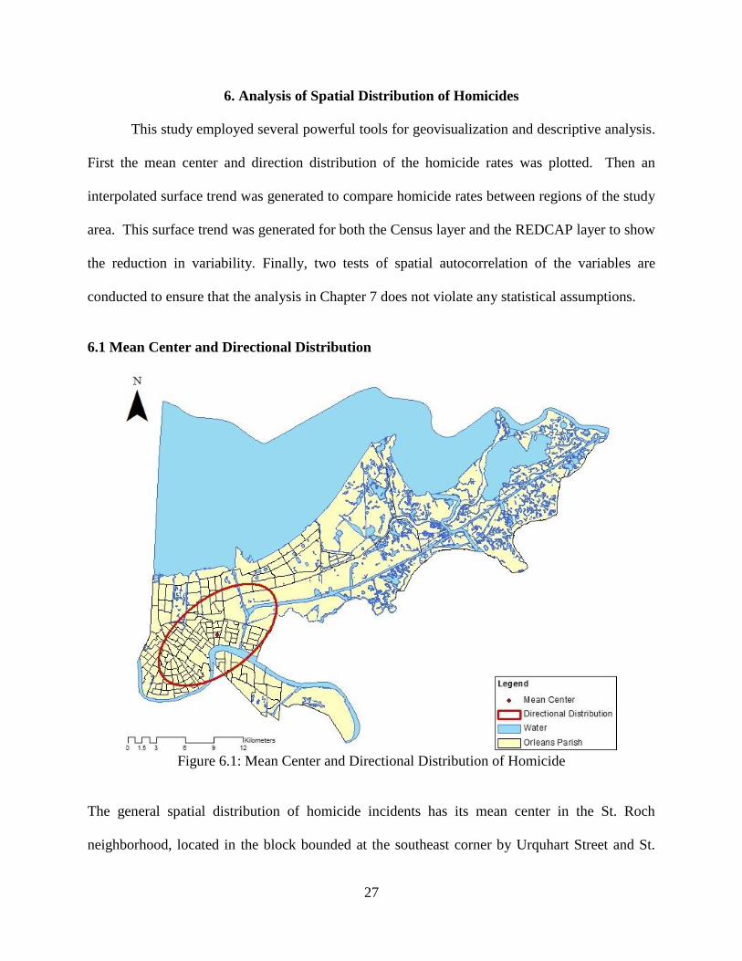
Figure 6.1: Mean Center and Directional Distribution of Homicide

The general spatial distribution of homicide incidents has its mean center in the St. Roch

neighborhood, located in the block bounded at the southeast corner by Urquhart Street and St.

28

Roch Avenue and bounded at the northwest corner by Spain Street and North Villere Street. The

direction distribution falls in an oblong ellipse from southwest to northeast of the Parish. This

descriptive analysis provides very little detail concerning the distribution of homicide, so more

complex analysis follows. Note that the mean center of incidents does not change based on the

spatial layer, whether it is census tracts or REDCAP regions.

6.2 Geovisualization of Homicide Rates

To provide a clearer picture of the spatial patterns of homicide, a surface displaying the

trends in homicide rates across the census tracts and the REDCAP layer was generated. To do

so, the ArcGIS Feature to Point tool was used to create tract and region centroids for the study

area, in which the homicide rate is encoded. Using the Geostatistical Analyst plugin for ArcGIS,

the Inverse Distance Weighting (IDW) method, which is a deterministic method of interpolation,

was applied with the following results:

Table 6.1: Prediction Error of the IDW Operation

Census New Area

Observations 173 50

Power 7 7

Mean -112.84 15.99

RMS 1140.77 246.11

Seventh-order polynomials were used for the operation. The extreme variability in the

homicide rates in the census layer is shown by both the large divergence in the average standard

error (mean) and the Root Mean Square (RMS) of the continuously varying function. The

regionalization operation reduced the variability in rates, as demonstrated by the mean and RMS

of the function for the REDCAP layer. This is also demonstrable by the geovisualization of the

function by the output rasters in Figures 6.2 and 6.3.

29

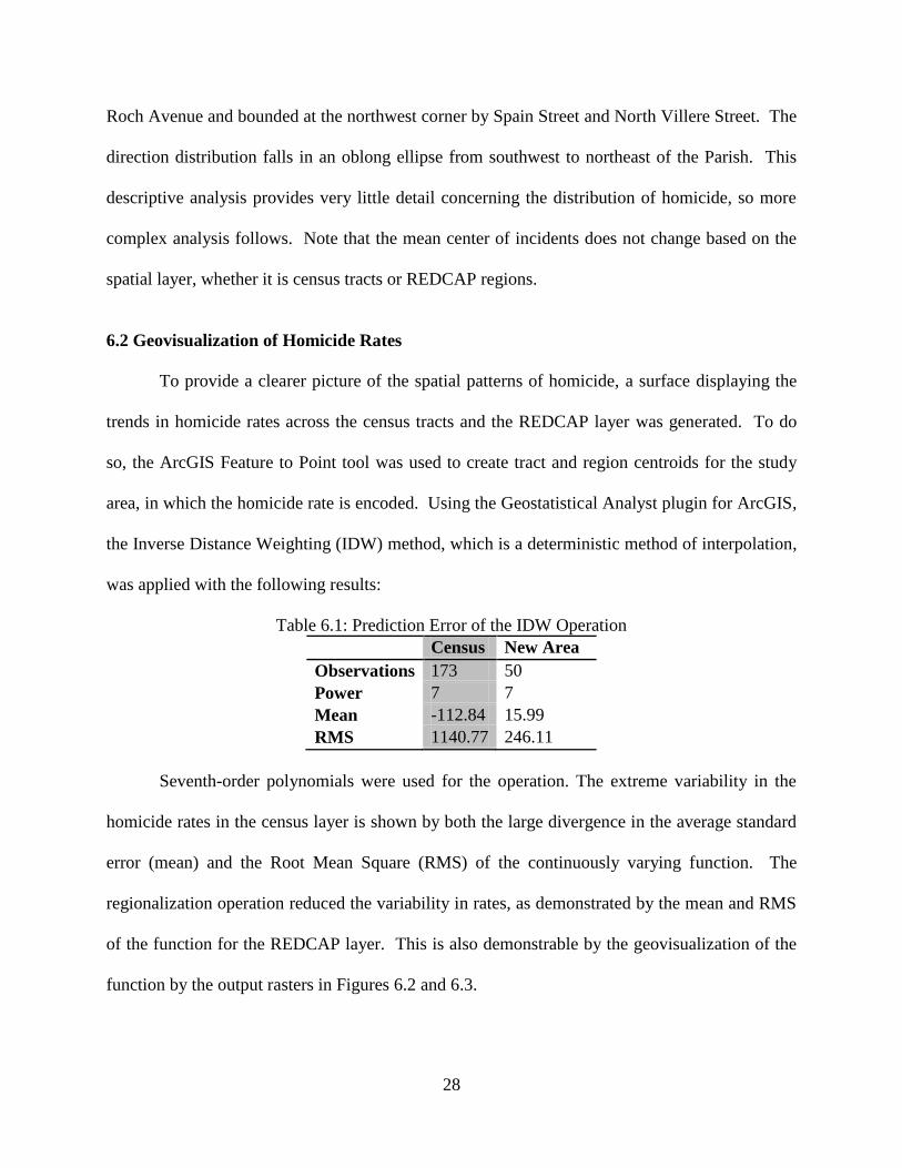
Figure 6.2: Homicide Rate Trends in the Census Layer

The highest observed homicide rate trend is City Park, which can be identified as the large dark

area in the northwest corner of the study area. High homicide rates are also observed in a swath

starting in Central City (southwest of the Central Business District), proceeding northeast

through the CBD, and continuing through the Mid-City, Bywater, and Lower Ninth Ward

neighborhoods. Enclaves of high rates are observed in the Hollygrove, Lakewood, and Mid-City

neighborhoods. In New Orleans East, high rates occur in the Lake Forest and Venetian isles

neighborhoods.

Conversely, low homicide rate trends are observed in the Uptown/Carollton area, which

is in the southwestern most portion of the city. Lakeview (northwest) also enjoys typically low

30

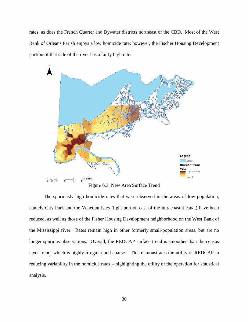
rates, as does the French Quarter and Bywater districts northeast of the CBD. Most of the West

Bank of Orleans Parish enjoys a low homicide rate; however, the Fischer Housing Development

portion of that side of the river has a fairly high rate.

Figure 6.3: New Area Surface Trend

The spuriously high homicide rates that were observed in the areas of low population,

namely City Park and the Venetian Isles (light portion east of the intracoastal canal) have been

reduced, as well as those of the Fisher Housing Development neighborhood on the West Bank of

the Mississippi river. Rates remain high in other formerly small-population areas, but are no

longer spurious observations. Overall, the REDCAP surface trend is smoother than the census

layer trend, which is highly irregular and coarse. This demonstrates the utility of REDCAP in

reducing variability in the homicide rates – highlighting the utility of the operation for statistical

analysis.

31

6.3 Spatial Autocorrelation of the Variables

The Moran’s I statistic (Moran 1950) is used to create an index of spatial autocorrelation

in the data, that is, to test whether there is spatial dependency in the variables. The tool is

included in the GIS and measures values of features and their locations to detect the degree of

clustering or dispersion. An index, z-score, and p-value are calculated. In the case of the

Moran’s test, the null hypothesis is that data values occur at random. The scores are interpreted

according to Table 7.1.

Table 6.2: Interpretation of Moran’s I Output

Positive Index Similar values cluster

Negative Index Dissimilar values cluster

Zero Index Total Randomness

Positive z-score Values are clustered and not random

Negative z-score Values are dispersed and not random

Insignificant p-value No assumption other than random

The first Moran’s test was conducted with the homicide rates in both the census and REDCAP

layers with a distance threshold of 5000 meters. As we can see from table 5.2, the rates in in the

census layer appear to occur at random; conversely, rates in the REDCAP layer are clustered.

Table 6.3: Moran’s I for Homicide Rates

Census New Areas

Index: 0.01 0.13

z-score: 1.06 3.30

p-value (< .05): 0.29 0.00

The insignificance of the test for the census layer means that the rates appear to occur completely

randomly, which, given the spatial pattern of homicide incidences in Chapter 3, is a poor

assumption. The REDCAP test is significant with a positive index and z-score, meaning that

homicides do cluster. We should expect to see a clustering of homicides because, although

homicide is statistically a rare event, it is rarely a random one in New Orleans – especially given

the assumption of retaliatory homicides. No one paying attention to homicide patterns in the city

32

can assume that these patterns are independent observations. Here the REDCAP regionalization

provides us patterns in the data that would otherwise be obscured by small populations and

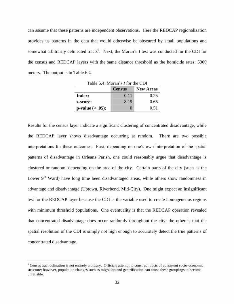
somewhat arbitrarily delineated tracts6. Next, the Moran’s I test was conducted for the CDI for

the census and REDCAP layers with the same distance threshold as the homicide rates: 5000

meters. The output is in Table 6.4.

Table 6.4: Moran’s I for the CDI

Census New Areas

Index: 0.11 0.25

z-score: 8.19 0.65

p-value (< .05): 0 0.51

Results for the census layer indicate a significant clustering of concentrated disadvantage; while

the REDCAP layer shows disadvantage occurring at random. There are two possible

interpretations for these outcomes. First, depending on one’s own interpretation of the spatial

patterns of disadvantage in Orleans Parish, one could reasonably argue that disadvantage is

clustered or random, depending on the area of the city. Certain parts of the city (such as the

Lower 9th

Ward) have long time been disadvantaged areas, while others show randomness in

advantage and disadvantage (Uptown, Riverbend, Mid-City). One might expect an insignificant

test for the REDCAP layer because the CDI is the variable used to create homogeneous regions

with minimum threshold populations. One eventuality is that the REDCAP operation revealed

that concentrated disadvantage does occur randomly throughout the city; the other is that the

spatial resolution of the CDI is simply not high enough to accurately detect the true patterns of

concentrated disadvantage.

6 Census tract delination is not entirely arbitrary. Officials attempt to construct tracts of consistent socio-economic

structure; however, population changes such as migration and gentrification can cause these groupings to become

unreliable.

33

6.4 Local Test of Spatial Autocorrelation

Anselin (1995) developed a local version of the Moran’s I referred to as Local Indicators

of Spatial Association (LISA) to test for spatial clusters and spatial outliers in a given data set.

When performed on each variable, this test allows assessment of spatial autocorrelation when

maps are compared. The test was performed on the homicide rate and CDI for both layers.

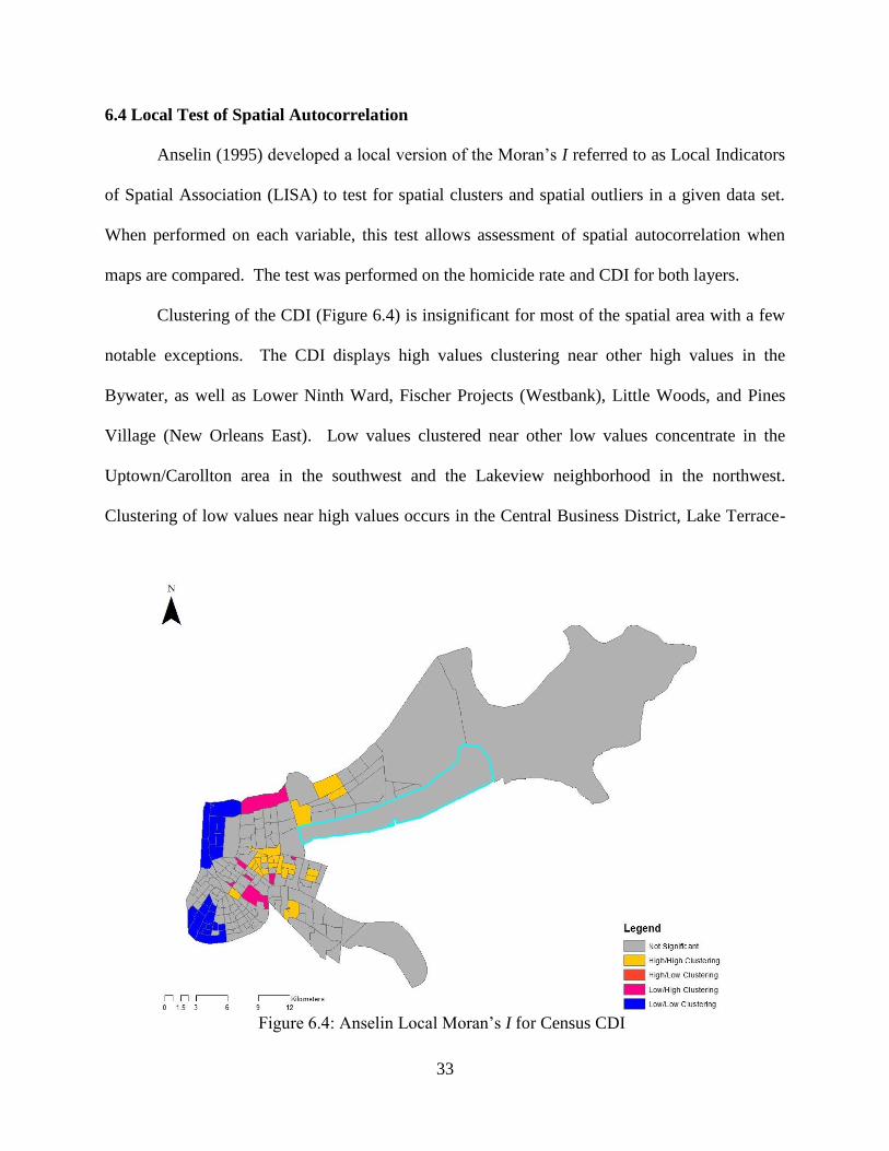
Clustering of the CDI (Figure 6.4) is insignificant for most of the spatial area with a few

notable exceptions. The CDI displays high values clustering near other high values in the

Bywater, as well as Lower Ninth Ward, Fischer Projects (Westbank), Little Woods, and Pines

Village (New Orleans East). Low values clustered near other low values concentrate in the

Uptown/Carollton area in the southwest and the Lakeview neighborhood in the northwest.

Clustering of low values near high values occurs in the Central Business District, Lake Terrace-

Figure 6.4: Anselin Local Moran’s I for Census CDI

34

Oaks neighborhood (New Orleans East), and patches throughout the Mid-City area.

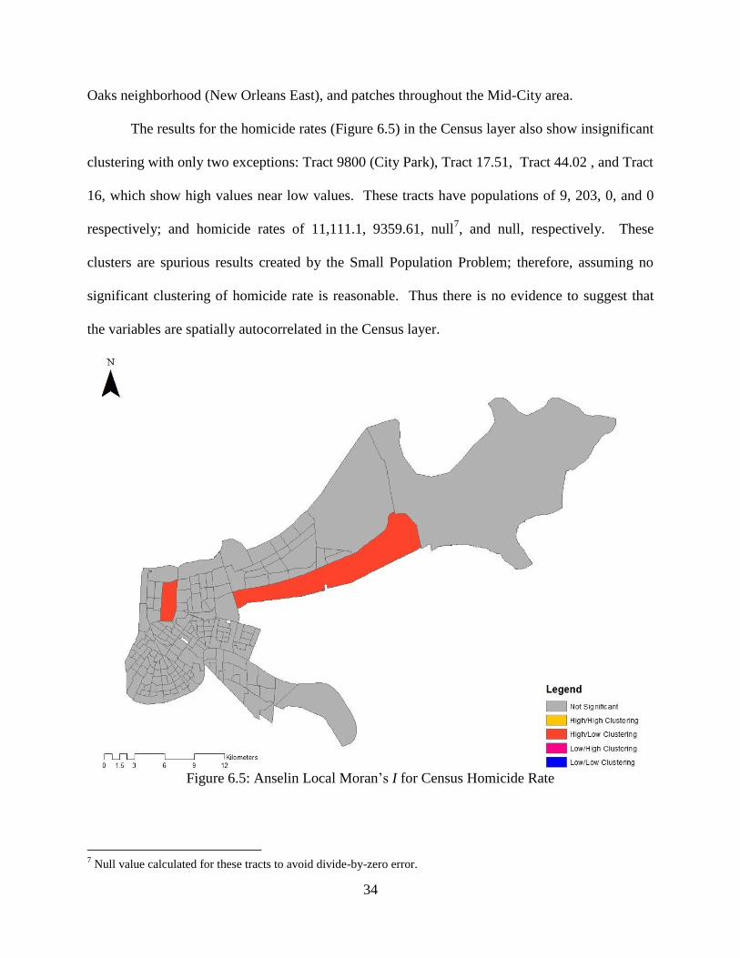
The results for the homicide rates (Figure 6.5) in the Census layer also show insignificant

clustering with only two exceptions: Tract 9800 (City Park), Tract 17.51, Tract 44.02 , and Tract

16, which show high values near low values. These tracts have populations of 9, 203, 0, and 0

respectively; and homicide rates of 11,111.1, 9359.61, null7, and null, respectively. These

clusters are spurious results created by the Small Population Problem; therefore, assuming no

significant clustering of homicide rate is reasonable. Thus there is no evidence to suggest that

the variables are spatially autocorrelated in the Census layer.

Figure 6.5: Anselin Local Moran’s I for Census Homicide Rate

7 Null value calculated for these tracts to avoid divide-by-zero error.

35

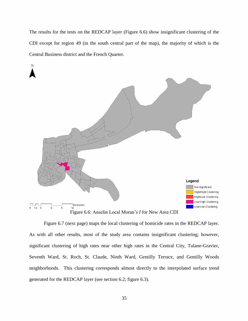
The results for the tests on the REDCAP layer (Figure 6.6) show insignificant clustering of the

CDI except for region 49 (in the south central part of the map), the majority of which is the

Central Business district and the French Quarter.

Figure 6.6: Anselin Local Moran’s I for New Area CDI

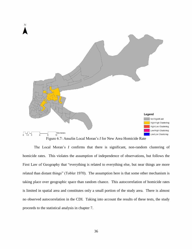
Figure 6.7 (next page) maps the local clustering of homicide rates in the REDCAP layer.

As with all other results, most of the study area contains insignificant clustering; however,

significant clustering of high rates near other high rates in the Central City, Tulane-Gravier,

Seventh Ward, St. Roch, St. Claude, Ninth Ward, Gentilly Terrace, and Gentilly Woods

neighborhoods. This clustering corresponds almost directly to the interpolated surface trend

generated for the REDCAP layer (see section 6.2; figure 6.3).

36

Figure 6.7: Anselin Local Moran’s I for New Area Homicide Rate

The Local Moran’s I confirms that there is significant, non-random clustering of

homicide rates. This violates the assumption of independence of observations, but follows the

First Law of Geography that “everything is related to everything else, but near things are more

related than distant things” (Tobler 1970). The assumption here is that some other mechanism is

taking place over geographic space than random chance. This autocorrelation of homicide rates

is limited in spatial area and constitutes only a small portion of the study area. There is almost

no observed autocorrelation in the CDI. Taking into account the results of these tests, the study

proceeds to the statistical analysis in chapter 7.

37

7. Analysis of Association between Concentrated Disadvantage and Homicide Rate

The experimental spatial analysis in this study employs several different methods. First a

simple OLS regression analysis was performed to test whether the homicide rate can be

explained by concentrated disadvantage – again for both layers. Last, a Geographically

Weighted Regression was used to test this relationship in a spatially disaggregated manner. The

outputs of these analyses are visualized and discussed.

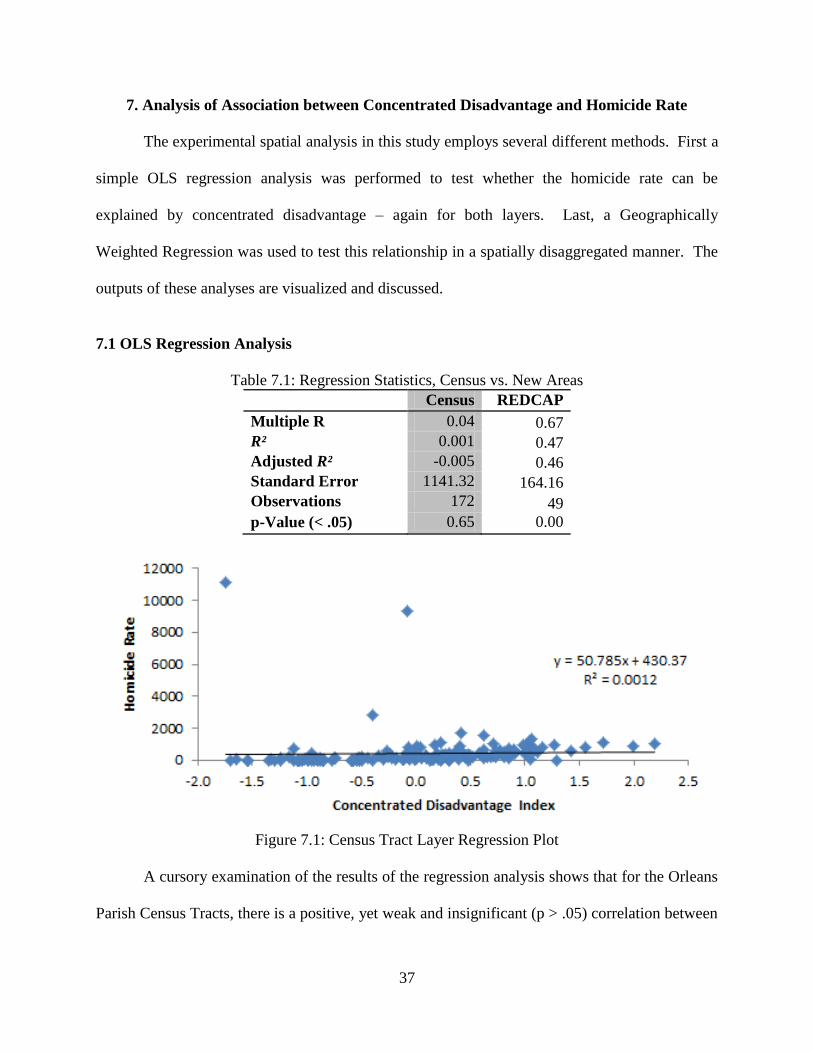
7.1 OLS Regression Analysis

Table 7.1: Regression Statistics, Census vs. New Areas

Census REDCAP

Multiple R 0.04 0.67

R² 0.001 0.47

Adjusted R² -0.005 0.46

Standard Error 1141.32 164.16

Observations 172 49

p-Value (< .05) 0.65 0.00

Figure 7.1: Census Tract Layer Regression Plot

A cursory examination of the results of the regression analysis shows that for the Orleans

Parish Census Tracts, there is a positive, yet weak and insignificant (p > .05) correlation between

38

the homicide rates and the CDI. The results of the analysis do not support the hypothesis that

homicide rates can be explained by levels of concentrated disadvantage. Note that this analysis

does not include observations at two census tracts; zero population in these prevented a homicide

rate from being calculated. We also observe the Small Population Problem skewing the

homicide rates at low levels (≤ 0) of disadvantage. The model is also a very poor fit with an R²

value of less than .01 (and a negative adjusted R² value).

Figure 7.2: REDCAP Layer Regression Plot

Regression results on the REDCAP layer show a positive and significant (p < .05)

correlation between the homicide rates and the CDI. The results of the analysis support the

hypothesis that homicide rates are associated with the level of concentrated disadvantage, and the

relationship is statistically significant. The REDCAP operation allowed the model to account for

more of the variance than the census tracts alone because the regionalization created more

reliable observations. The R² (.47) is a significant improvement in fit over the Census layer

(.001). The adjusted R² (.46) is close to the original, indicating a good fit and lack of shrinkage.

39

7.2 Geographically Weighted Regression: Evaluating Spatial Non-stationarity

One way to test correlation between the variables without regard to their spatial

autocorrelation is to use a tool provided in the GIS called Geographically Weighted Regression

(GWR) developed by Brundson, Fotheringham, and Charlton (1998). This method generates a

regression model at each feature in the layer rather than at the aggregate, which avoids the

problem of spatial dependency in the variables, whether or not we expect that dependency to

appear in one or all of them. An adaptive kernel was specified to create the model based on

nearest neighbors, rather than a fixed kernel, which specifies the model for a certain distance.

Results can be interpreted in a fashion nearly equal to a linear regression. An additional benefit

is the availability to use the Moran’s I on the local regression residuals as a test of robustness

(Mei and Zhang 2000); a randomly dispersed residual set generally indicates a properly-specified

model. The Sigma value may be interpreted as the standard deviation of the local residuals. The

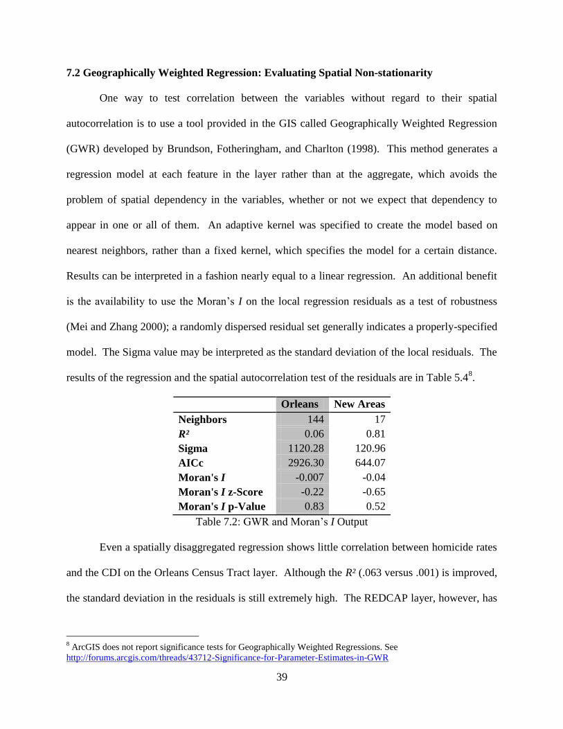
results of the regression and the spatial autocorrelation test of the residuals are in Table 5.48.

Orleans New Areas

Neighbors 144 17

R² 0.06 0.81

Sigma 1120.28 120.96

AICc 2926.30 644.07

Moran's I -0.007 -0.04

Moran's I z-Score -0.22 -0.65

Moran's I p-Value 0.83 0.52

Table 7.2: GWR and Moran’s I Output

Even a spatially disaggregated regression shows little correlation between homicide rates

and the CDI on the Orleans Census Tract layer. Although the R² (.063 versus .001) is improved,

the standard deviation in the residuals is still extremely high. The REDCAP layer, however, has

8 ArcGIS does not report significance tests for Geographically Weighted Regressions. See

http://forums.arcgis.com/threads/43712-Significance-for-Parameter-Estimates-in-GWR

40

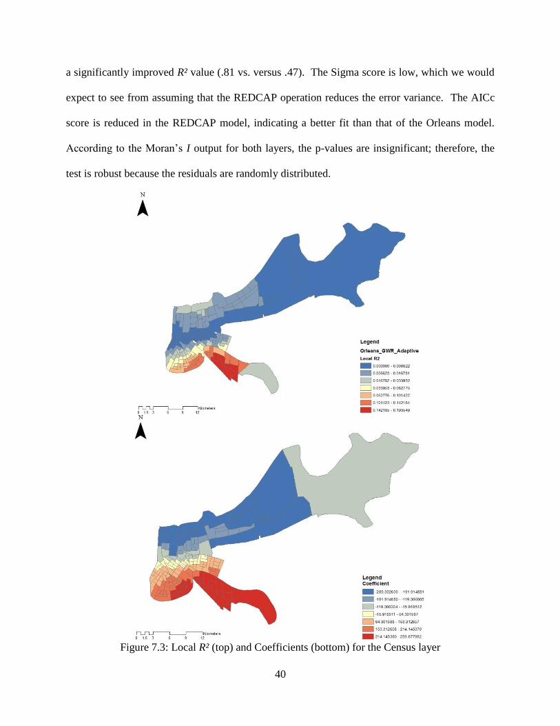
a significantly improved R² value (.81 vs. versus .47). The Sigma score is low, which we would

expect to see from assuming that the REDCAP operation reduces the error variance. The AICc

score is reduced in the REDCAP model, indicating a better fit than that of the Orleans model.

According to the Moran’s I output for both layers, the p-values are insignificant; therefore, the

test is robust because the residuals are randomly distributed.

Figure 7.3: Local R² (top) and Coefficients (bottom) for the Census layer

41

The GWR model for the census layer accounts for a very low percentage of the

dependent variable. In addition, the spatial pattern of the local R² (Figure 7.3) seems to exhibit a

cascading north-south pattern that does not make very much sense. The coefficients are largely

negative which indicates that there is no relationship between the independent and dependent

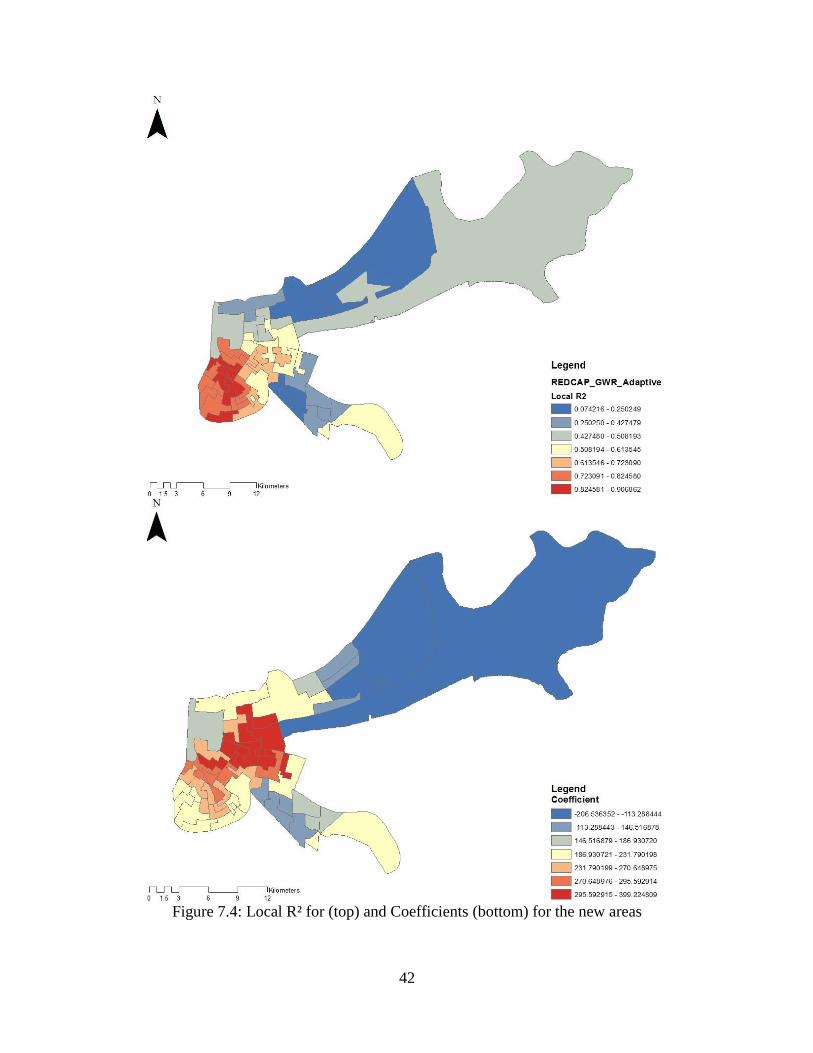
variables. However, in the REDCAP layer (figure 7.4), the smallest regions by area (indicating

higher population density) have the highest R² values (> .5). The coefficients are positive for the

vast majority of the map. Negative coefficients are seen in New Orleans East and the western

portion of the West Bank region. The highest coefficients are seen in those areas with the

highest homicide rate trends (see section 6.2). Figure 7.4 provides information about both the

degree of the non-stationarity of the relationships between the variables and the ability of the

REDCAP process to reveal patterns in the data that would otherwise be hidden.

Several conclusions can be drawn from the GWR process in this case study. That the

homicide rates in the Census layer are extremely unreliable has been established; spatial non-

stationarity cannot be evaluated accurately at the bandwidth. Although the model was shown to

be properly specified, it has a poor goodness of fit. Additionally, the coefficients show a

negative relationship between the variables, regardless of what the linear regression stated. The

model was discussed here mostly for comparison purposes because the GWR is an effective tool

at evaluating the non-stationarity in the REDCAP layer. The R² is significantly improved over

the linear regression and the coefficients are largely positive. The model is a far better fit than of

the Census layer. The GWR shows us that the homicide rate’s dependence on the CDI is

spatially correlated in the REDCAP layer.

42

Figure 7.4: Local R² for (top) and Coefficients (bottom) for the new areas

43

The maps of the local R² and coefficients for the census layer tell us nothing about the

spatial pattern of correlation. This is likely due to the confounding of patterns in the data due to

the issues created by the Small Population Problem and the MAUP. However, an examination of

the local R² and coefficients in the REDCAP layer provides more information about the spatial

non-stationarity of the correlation between the homicide rate and the CDI. First, the lowest fit of

the model (R² ≤ .5) and lowest coefficients tend to occur in the same place: on the peripheral

areas in the northwest, north, east, and south central. Second, the best fit of the model (≥ .51)

occurs in the southwest, central, and far southeast portions of the study area. More interesting is

the fact that the regression coefficients are highest both in the areas surrounding the highest

homicide rate trend (Figure 6.3) but also the areas surrounding those where the homicide rate is

spatially autocorrelated (Figure 6.7). This indicates that the correlation in the REDCAP layer is

not likely the result of random chance, as homicide events are probably not autocorrelated by

random chance, but because they are in fact a consequence of concentrated disadvantage in that

area. For the areas of lower correlation, there is no clear explanation of this phenomenon other

than that the homicide rate might be the result of other factors than Concentrated Disadvantage,

or other indicators for which the CDI did not account.

44

8. Conclusion

This study has demonstrated, first and foremost, the significant problem of homicide in

New Orleans, Louisiana. The city frequently holds the title of the murder capital of the United

States – a fact regretted not only by local residents who hold the city so dear to their hearts, but

also by the city’s political and business leaders. The first objective of this study was to provide

an explanation for the cause of the problem. A large body of sociological research demonstrates

that high levels of social disorganization, indicated by concentrated socioeconomic disadvantage,

tends to increase violent crime rates, including those of homicide. The second objective of this

study was to assess the viability of the Regionalization with Dynamically Constrained

Agglomerative Clustering and Partitioning (REDCAP) method of automatic region building as a

tool for mitigating the statistical issues created by the Modifiable Areal Unit Problem and the

Small Population Problem. Thus there were two hypotheses.

The first hypothesis was that there is a positive and significant relationship between

Concentrated Disadvantage and the homicide rate in the study area. This hypothesis was not

confirmed for the Orleans Parish census tract layer; however, it was confirmed in the newly

constructed region layer. The second hypothesis was that the REDCAP successfully mitigates

problems with homicide rate calculations in census tracts. This was confirmed by the reduction

in variability in the variables used in regression analyses, as well as the significant fact that the

first hypothesis was confirmed for the post-REDCAP regions, but not the census layer.

The concentrated disadvantage in certain neighborhoods of the city is a clear explanation

for the homicide rate. When factors such as segregation, poverty, single-parent families, and

high unemployment concentrate spatially, disadvantage is so concentrated that the very

organization of the society breaks down. This in turn leads to poor outcomes in mental health of

45

residents and trust between residents. This combined with low level of trust of the police force

results in residents seeking informal means of conflict resolution, specifically murder. This

study has clearly established the link between concentrated disadvantage and the homicide rate

in New Orleans. Regression analyses showed a high correlation between the two in the

REDCAP layer, especially in the results of the Geographically Weighted Regression which

reported an R² value of .81.

In addition, this study has shown the efficacy of the Regionalization with Dynamically

Constrained Agglomerative Clustering and Partitioning (REDCAP) method of automatic region

building as a tool for homicide research. REDCAP provides an efficient solution to the problems

that result from the Small Population Problem, in particular, the creation of unstable homicide

rate observations calculated in arbitrarily delineated census tracts. By creating more stable

homicide rates, REDCAP allows the analysis of patterns that would otherwise be hidden within

the data sets. REDCAP’s viability as a tool in homicide research is demonstrated throughout the

study. Its utility was first demonstrated by the creation of a more stable and reliable interpolated

surface trend with lower variation than the census layer. Most importantly, it allowed the first

hypothesis to be confirmed after its use, as it resulted in the reductions in the variability in the

variables used in the regression analyses. This demonstrates its potential for use in more

rigorous statistical analysis, such as those with factor analysis or multivariate regressions. For

example, REDCAP can enable researchers to conduct exploratory regressions in the ArcGIS

package with several variables to determine which of those in the Concentrated Disadvantage

Index are more salient in explaining the homicide rate.

This study also provides implications for public policy decisions. By providing more

reliable statistics concerning the homicide problem, the study provides better information to

46

those in positions of responsibility in public policy to make more informed decisions regarding

the homicide problem.

There were 193 murders not including justifiable homicides and accidents in 2012 – a

roughly 3% decrease from 2011 (Vargas 2012). Police investigated 42 murders in the first

quarter of 2013, most of which were in those areas shown in this study to have a high correlation

between Concentrated Disadvantage and homicide. The fact that homicide exhibits a fairly

consistent spatial pattern allows government to target certain areas with different policing

methods, such as community-oriented policing. The New Orleans Police Department (NOPD)

has started employing this method in some of the most disadvantaged, most deadly

neighborhoods in the city (Elliott 2012). This study shows specifically which areas should be

targeted by these methods. However, it is unclear whether this new action by the NOPD has had

a significant effect so far. It is the sincere hope of this researcher that the results of this study

will help officials to stem the homicide problem in New Orleans, Louisiana.

47

References

Anselin, Luc. (1995). “Local Indicators of Spatial Association – LISA” Geographical Analysis,

27, 93-115.

Bellair, Paul E. (1997). “Social Interaction and Community Crime: Examining the Importance

of Neighbor Networks.” Criminology, 35, 677-704.

Black, R., L. Sharp, and J. D. Urquhart. (1996). “Analyzing the spatial distribution of disease

using a method of contructing geographical areas of approximately equal population size.”

In Methods for investigating localized clustering of disease, edited by P.E. Alexander and P.

Boyle, 28-39. Lyon: International Agency for Research on Cancer.

Brundson, Chris, Stewart Fotheringham, and Martin Charlton. (1998). “Geographically

weighted regression—modeling spatial non-stationarity.” Journal of the Royal Statistical

Society, Series D (The Statistician), 47, 431-443.

Cohen, Lawrence E. and Marcus Felson. (1979). “Social Change and Crime Rate Trends: A

Routine Activity Approach.” American Sociological Review, 44, 588-608.

Consejo ciudadano para la Seguridad Pública y Justicia Penal A.C. (CCSPJP). (2011). “San

Pedro sula, la ciudad más violenta del mundo; Juárez, la segunda.” Consejo ciudadano para

la Seguridad Pública y Justicia Penal A.C, January 11. Accessed November 30, 2012.

http://www.seguridadjusticiaypaz.org.mx/sala-de-prensa/541-san-pedro-sula-la-ciudad-mas-

violenta-del-mundo-juarez-la-segunda

De Coster, Stacy, Karen Heimer, and Stacy M. Wittrock. (2006). “Neighborhood Disadvantage,

Social Capital, Street Context, and Youth Violence.” The Sociological Quarterly, 47, 723-

753.

Elliott, Debbie. (2012). “New Orleans Struggles With Murder Rate, and Trust,” National Public

Radio, July 5. Accessed November 30, 2012.

http://www.npr.org/2012/07/05/155986277/new-orleans-struggles-with-murder-rate-and-trust

Greater New Orleans Community Data Center (GNOCDC). (2012). “Neighborhood statistical

data profiles.” New Orleans: Greater New Orleans Community Data Center. Accessed

March 23, 2013. http://gnocdc.org/NeighborhoodData/Orleans.html.

Guo, Diansheng. (2008). “Regionalization with dynamically constrained agglomerative

clustering and partitioning (REDCAP).” International Journal of Geographical Information

Science, 22, 801-823.

Guo, Diansheng and Hu Wang. (2011). “Automatic Region Building for Spatial Analysis.”

Transactions in GIS, 15, 29-45.

48

Haining, Robert, Stephen Wise, and Marcus Blake. (1994). “Construction regions for small area

analysis: material deprivation and colorectal cancer.” Journal of Public Health, 16, 429-438.

Haining, Robert, Stephen Wise, and Jingsheng Ma. (1998). “Exploratory Spatial Data Analysis

in a Geographic Information System Environment.” Journal of the Royal Statistical Society,

Series D (The Statistician), 47, 457-469.

Harrel, A. and C. Gouvis. (1994). “Predicting neighborhood risk of crime: Report to the

National Institute of Justice.” Washington D.C.: The Urban Institute.

Hipp, John R. (2010). “A Dynamic View of Neighborhoods: The Reciprocal Relationship

between Crime and Neighborhood Structural Characteristics.” Social Problems, 57, 205-

230.

Hoffman, John P. (2003). “A Contextual Analysis of Differential Association, Social Contorl,

and Strain Theories of Delinquency.” Social Forces, 8, 753-785.

Jervis, Rick. (2008). “New Orleans homicides up 30% over ’06 level.” USA Today, January 3.

Accessed November 30, 2012. http://usatoday30.usatoday.com/news/nation/2008-01-02-

Orleanscrime_N.htm

Kawachi, Ichiro, Bruce P. Kennedy, and Richard G. Wilkinson. (1999). “Crime: social

disorganization and relative deprivation.” Social Science & Medicine, 48, 719-731.

Krivo, Lauren J. and Ruth D. Peterson. (1996). “Extremely Disadvantaged Neighborhoods and

Urban Crime.” Social Forces, 75, 619-648.

Krivo, Lauren J. and Ruth D. Peterson. (2000). “The Structural Context of Homicide:

Accounting for Racial Differences in process.” American Sociological Review, 65, 547-559.

Krivo, Lauren J., Ruth D. Peterson, Helen Rizzo, and John R. Reynolds. (1998). “Race,

Segregation, and the Concentration of Disadvantage: 1980-1990.” Social Problems, 45, 61-

80.

Krupa, Michelle. (2012). "New Orleans tourism breaks record in 2011," The Times-Picayune,

March 26. Accessed February 15, 2013.

http://www.nola.com/politics/index.ssf/2012/03/new_orleans_tourism_breaks_rec.html

Kubrin, Charis E. and Ronald Weitzer. (2003). “Retaliatory Homicide: Concentrated

Disadvantage and Neighborhood Culture.” Social Problems, 50, 157-180.

Lam, Nina Siu-Ngan and Kam-biu Liu. (1996). “Use of Space-Filling Curves in Generating a

National Rural Sampling Frame for HIV/AIDS Research.” Professional Geographer, 48,

321-332.

49

Land, Kenneth C., Patricia L. McCall, and Lawrence E. Cohen. (1990). “Structural Covariates

of Homicide Rates: Are There Any Invariances across Time and Social Space?” American

Journal of Sociology, 95, 922-63.

Land, Kenneth C., Patricia L. McCall, and Daniel S. Nagin. (1996). “A Comparison of Poisson,

Negative Binomial, and Semiparametric Mixed Poisson Regression Models: With Empirical

Applications to Criminal Careers Data.” Sociological Methods and Research, 24, 387-442.

Lee, Matthew R. (2000). “Concentrated Poverty, Race, and Homicide.” The Sociological

Quarterly, 41, 189-206.

Maggi, Laura. (2012). “New Orleans homicides jump by 14 percent in 2011,” The Times-

Picayune, January 1. Accessed November 30, 2012.

http://www.nola.com/crime/index.ssf/2012/01/new_orleans_homicides_jump_by.html

Martin, Michel. (2012). “Understanding New Orleans’ Murder Epidemic,” National Public

Radio, May 29. Accessed November 30, 2012.

http://www.npr.org/2012/05/29/153918840/understanding-new-orleans-murder-epidemic

McCollam, Douglas. (2011). “In America's Murder Capital, the Killing Is Personal; The New

Orleans homicide rate is 10 times the national average. But gangs and drugs don't explain it,”

Wall Street Journal, November 12. Accessed November 30, 2012.

http://online.wsj.com/article/SB10001424052970204224604577028463391009838.html

Messner, Steven F., Luc Anselin, Robert D. Baller, Darnell F. Hawkins, Glenn Deane, and

Stewart E. Tolnay. (1999). “The Spatial Patterning of County Homicide Rates: An

Application of Exploratory Spatial Data Analysis.” Journal of Quantitative Criminology, 15,

423-450.

Morenoff , Jeffrey D. and Robert J. Sampson. (1997). “Violent Crime and the Spatial Dynamics

of Neighborhood Transition: Chicago, 1970-1990.” Social Forces, 76, 31-64.

Mu, Lan and Fahui Wang. (2008). “A Scale-Space Clustering Method: Mitigating the Effect of

Scale in the Analysis of Zone-Based Data.” Annals of the Association of American

Geographers, 98, 85-101.

New Orleans Convention and Visitors Bureau (NOCVB). "The Power of Tourism in New

Orleans." New Orleans Convention and Visitors Bureau Press Kit. Accessed February 15,

2013. http://www.neworleanscvb.com/press-media/press-kit/power-tourism/

Newkirk, Margaret. (2012). “New Orleans Murder Rate Climbs as City Begins Overhaul of

Police,” Bloomberg, August 9. Accessed November 30, 2012.

http://www.bloomberg.com/news/2012-08-10/new-orleans-murder-rate-climbs-as-city-

begins-overhaul-of-police.html

50

Openshaw, Stan. (1984). “The Modifiable Areal Unit Problem.” Concepts and Techniques in

Modern Geography, 38, 1-41.

Osgood, D. Wayne. (2000). “Poisson-Based Regression Analysis of Aggregate Crime Rates.”

Journal of Quantitative Criminology, 16, 21-43.

Osgood, D. Wayne and Jeff M. Chambers. (2000). “Social Disorganization outside the

Metropolis: An Analysis of Rural Youth Violence.” Criminology, 38, 81-116.

Peterson, Ruth D. and Lauren J. Krivo. (1999). “Racial Segregation, the Concentration of

Disadvantage, and Black and White Homicide Victimization.” Sociological Forum, 14, 465-

493.

Ripley, Amanda. (2006). “What Happened to the Gangs of New Orleans?” Time, May 22.

Accessed November 30, 2012.

http://www.time.com/time/magazine/article/0,9171,1194016,00.html

Ross, Catherine E. (2000). “Neighborhood Disadvantage and Adult Depression.” Journal of

Health and Social Behavior, 41, 177-187.

Ross, Catherine E., John Mirowsky, and Shana Pribesh. (2001). “Powerlessness and the

Amplification of Threat: Neighborhood Disadvantage, Disorder, and Mistrust.” American

Sociological Review, 66, 568-591.

Sampson, Robert J. and W. Byron Groves. (1989). “Community Structure and Crime: Testing

Social-Disorganization Theory.” American Journal of Sociology, 94, 774-802.

Sampson, Robert J., Stephen w. Raudenbush, and Felton Earls. (1997). “Neighborhoods and

violent Crime: A Multilevel Study of Collective Efficacy.” Science, 277, 918-924.

Shaw, Clifford R. and Henry D. McKay. (1942). Juvenile Delinquency in Urban Areas.

Chicago: University of Chicago Press.

Smith, Thomas Ruys. (2011). “New Orleans: The Big Uneasy,” History Today, 61. Accessed

November 30, 2012. http://www.historytoday.com/archive/history-today/2011/volume-61-

issue-8

South, Scott J. (2001). “The Geographic Context of Divorce: Do Neighborhoods Matter?”

Journal of Marriage and Family, 63, 755-766.

Swaroop, Sapna and Jeffrey D. Morenoff. (2006). “Building Community: The Neighborhood

Context of Social Organization.” Social Forces, 84, 1665-1695.

Taylor, Ralph B. (1996). “Neighborhood Responses to Disorder and Local Attachments: The

Systemic Model of Attachment, Social Disorganization, and Neighborhood Use Value.”

Sociological Forum, 11 (1), 41-74.

51

Taylor, Ralph B. and Jeanette Covington. (1993). “Community Structure Change and Fear of

Crime.” Social Problems, 40 (3), 374-397.

Tobler, Waldo. (1970). “A Computer Movie Simulating Urban Growth in the Detroit Region.”

Economic Geography, 46,: 234-240.

United States Census Bureau. (2010). 2010 American Community Survey Estimates. Accessed

October 1, 2012. http://factfinder2.census.gov/faces/nav/jsf/pages/index.xhtml

Vargas, Ramon Antonio. (2012). “Murders in New Orleans were slightly fewer in 2012 than in

2011.” The Times-Picayune, December 31. Accessed February 19, 2013.

http://www.nola.com/crime/index.ssf/2012/12/murders_in_new_orleans_were_sl.html

Wang, Fahui. (2005). “Job Access and Homicide Patterns in Chicago: An Analysis at Multiple

Geographic Levels Based on Scale-Space Theory.” Journal of Quantitative Criminology, 21,

195-217.

Wang, Fahui. (2012). “Why police and policing need GIS: An overview.” Annals of GIS, 18,

159-171.

Wang, Fahui, and Van O’Brien. (2005). “Constructing Geographic Areas for Analysis of

Homicide in Small Populations: Testing Herding-Culture-of-Honor Proposition.” In

Geographic Information Systems and Crime Analysis, edited by Fahui Wang, 84-100.

Hershey: IGI Global.

Wang, Fahui and Martin T. Arnold. (2008). “Localized income inequality, concentrated

disadvantage, and homicide.” Applied Geography, 28, 259-270.

Wang, Fahui, Diansheng Guo, and Sara McLafferty. (2012). “Constructing geographic areas for

cancer data analysis: A case study on late-stage breast cancer risk in Illinois.” Applied

Geography, 35, 1-11.

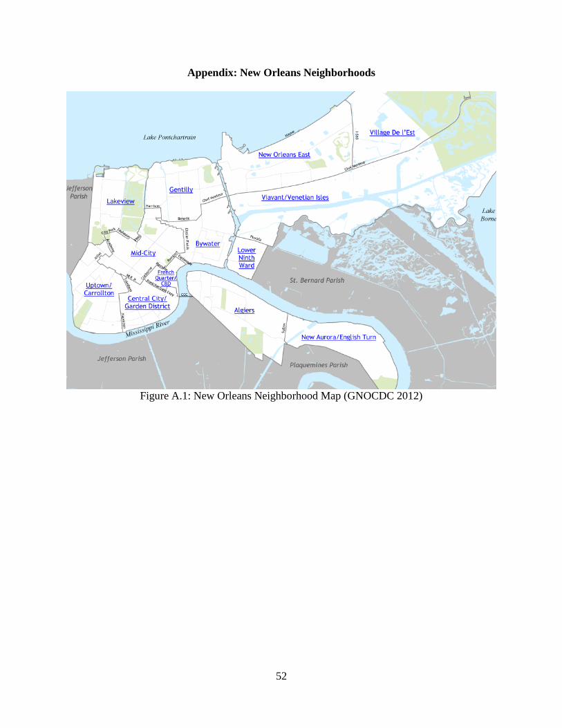
52

Appendix: New Orleans Neighborhoods

Figure A.1: New Orleans Neighborhood Map (GNOCDC 2012)

53

Vita

Lawrence Keenan Robert was born and raised in New Orleans, Louisiana. In 2008, he

received a Bachelor of Arts in International Studies with a concentration in Europe from

Louisiana State University. During that time, he studied the Italian and German languages; he

also conducted an in-depth geostrategic and geopolitical open-source intelligence analysis of the

2006-2007 phase of the Somali Civil War.

Mr. Robert traveled to Prague, Czech Republic in 2009 and earned a certification in

Teaching English as a Foreign Language. He taught students from the beginner through

advanced levels and gained a working knowledge of the Czech language. In 2010, he entered the

graduate program in Geography at Louisiana State University. In the spring 2012 semester, he

was a graduate assistant for Dr. Fahui Wang and Dr. Craig Colten. Mr. Robert lectured on the

Middle East, Central Asia, and the Caucasus in the Geography 1003: Africa and Asia

introductory course.

During his graduate studies, Mr. Robert conducted research on the indigenous religions

of Kurdistan, the geography of the European Monetary Union, geostrategy in Central Asia,

pipeline geopolitics in the South Caucasus and Central Asia, the Post-Soviet wars, and the death

of the Svan language. He also independently studied the Georgian language and the culture of

Georgia. In the summer of 2012, he returned to Georgia to conduct independent research on

cultural and political ecology, vernacular architecture, religion, gender, transit, immigration,

urbanization, infrastructure, and security. He also gained a limited working knowledge of the

Georgian language as well as beginner proficiency in the Russian language.

Mr. Robert expects to earn a Master of Science in Geography in the spring of 2013. He

has relocated to the District of Columbia to seek employment in service of the United States.