Constructing the Post-War Housing Boom

Matthew Chambers, Towson UniversityCarlos Garriga, FRB of St. Louis

Don Schlagenhauf, FRB of St. Louis

Interaction between Housing and the Economy, HumboltUniversity, Germany

June 2015

Postwar Housing Boom 1940-60: Ownership and Prices

1920 1930 1940 1950 1960 1970 1980 199030

40

50

60

70

80

90

1940s Boom1940s Boom

Year

Perc

ent

Home Ownership RateReal Home Price Index (H­P Filter)

Source: Shiller HPA and U.S. Census

Objective

I Objective: Understanding the positive co-movement betweenhome ownership and house prices in the postwar housing boom

I Methodology: Use a multi-sector equilibrium life-cycle modelwith housing tenure choice

I Decomposition: Identify the contribution of relevant factorsI Limitation: Focus on levels and not the transition

Literature: Focus ownership and little on prices

1. Demographics factors: Chevan (1989) estimates 50%2. Income Growth: Kain (1983) and Katona (1964) accountsfor most of it

3. Government Regulation of Housing markets

3.1 Regulation of Housing Finance: Yearn (1976), Chambers,Garriga, and Schlagenhauf (2009) estimates 50%

3.2 Assistance programs (VA): Fetters (2010) estimates 10%3.3 Taxation: Rosen and Rosen (1980) estimates 25%

Summary Findings

I Model performance: The baseline economy rationalizes theco-movement in prices and ownership.

I Main story: The model identifies a relative sectorialproductivity change of the goods sector over real estate as akey driver of the housing boom.

I Decomposition: Relative contribution of each factor

Contribution Ownership (%) House Prices (%)Demographics 5-8 1-2Income risk 12-57 0-1Govn’t Policy 3-4 0-14Housing finance 5-7 1-1.5

I) Summary of Relevant Factors

1) House Prices and Construction Cost Indices

1920 1925 1930 1935 1940 1945 1950 1955 1960 19650.5

0.6

0.7

0.8

0.9

1

1.1

1.2

1.3

1.4

1.5

Year

Inde

x (N

orm

aliz

ed 1

=194

0)

HPI (Shiller)CI Dept CommercetCI EH BoeckCI Engineer Record

Source: Alfred, St. Louis Fed

=⇒ House prices are in-line with construction costs

2) Demographics

Population Shares Family Size

2 0 3 0 4 0 5 0 6 0 7 0 8 0 9 00

0 .0 1

0 .0 2

0 .0 3

0 .0 4

0 .0 5

0 .0 6

0 .0 7

0 .0 8

0 .0 9

H o u s e h o ld  A g e

1 9 4 0

1 9 6 0

2 0 3 0 4 0 5 0 6 0 7 0 8 0 9 02

2 .5

3

3 .5

4

4 .5

T im e

Ave

rage

 Fam

ily 

Siz

e

1 9 4 0

1 9 6 0

Standard Deviation of Income (Source: IPUMS)

2) Demographics: Actual and Hypothetical Ownership

Ownership TotalExpression Rate Change

∑i∈I µi1940πi1940 44.53

∑i∈I µi1960πi1960 65.57 21.04

∑i∈I µi1960πi1940 47.47 2.94

∑i∈I µi1940πi1960 62.13 17.60

Data Source: United States Public Use Microdata Samples (IPUMS)

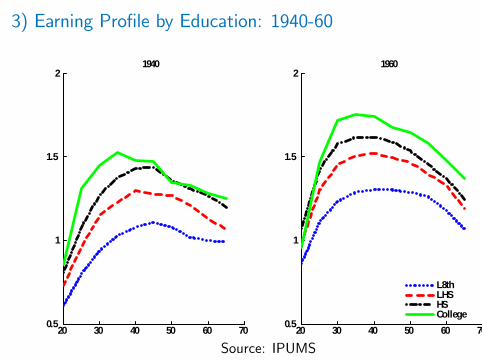
3) Earning Profile by Education: 1940-60

20 30 40 50 60 700.5

1

1.5

21940

20 30 40 50 60 700.5

1

1.5

21960

L8thLHSHSCollege

Source: IPUMS

3) Reduction Income Risk by Education: 1940-60

1940 1960

2 0 3 0 4 0 5 0 6 00 .5

0 .6

0 .7

0 .8

0 .9

1

1 .1

L e s s  th a n  8 th

K e r n e l

H is to g r a m

2 0 3 0 4 0 5 0 6 00 .5

0 .6

0 .7

0 .8

0 .9

1

1 .1

8 th ­ 1 1 th  G r a d e

K e r n e l

H is to g r a m

2 0 3 0 4 0 5 0 6 00 .5

0 .6

0 .7

0 .8

0 .9

1

1 .1

1 2 th  G r a d e

K e r n e l

H is to g r a m

2 0 3 0 4 0 5 0 6 00 .5

0 .6

0 .7

0 .8

0 .9

1

1 .1

C o lle g e

K e r n e l

H is to g r a m

2 0 3 0 4 0 5 0 6 00 .5

0 .6

0 .7

0 .8

0 .9

1

1 .1

L e s s  th a n  8 th

K e r n e l

H is to g r a m

2 0 3 0 4 0 5 0 6 00 .5

0 .6

0 .7

0 .8

0 .9

1

1 .1

8 th ­ 1 1 th  G r a d e

K e r n e l

H is to g r a m

2 0 3 0 4 0 5 0 6 00 .5

0 .6

0 .7

0 .8

0 .9

1

1 .1

1 2 th  G r a d e

K e r n e l

H is to g r a m

2 0 3 0 4 0 5 0 6 00 .5

0 .6

0 .7

0 .8

0 .9

1

1 .1

C o lle g e

K e r n e l

H is to g r a m

Standard Deviation of Income (Source: IPUMS)

4) Government Regulation of Housing Finance

I Prior Great Depression: The typical mortgage contract wascharacterized by

I a maturity of less than ten years,I a loan-to-value ratio of about 50 percent,I interest only with a balloon payment at expirationI Regional credit markets

I Post Great Depression (1940’s Boom): FHA introducesfixed rate mortgage

I longer maturity 20 to 30 yearsI higher LVT ratio (i.e. 80 percent, or 100 percent VA)I constant repayment over length loan (self-amortizing)I National credit markets (↓ decline in mortgage rates)

4) Mortgage Market Regulation: Interest rates

1900 1910 1920 1930 1940 1950 19602

2.5

3

3.5

4

4.5

5

5.5

6

Source: Grebler, Blank, and Winnick (1956)

Per

cent

MortgageBond

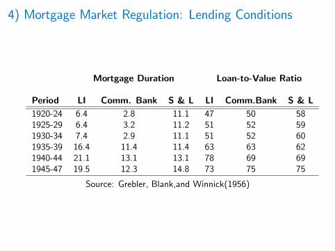
4) Mortgage Market Regulation: Lending Conditions

Mortgage Duration Loan-to-Value Ratio

Period LI Comm. Bank S & L LI Comm.Bank S & L1920-24 6.4 2.8 11.1 47 50 581925-29 6.4 3.2 11.2 51 52 591930-34 7.4 2.9 11.1 51 52 601935-39 16.4 11.4 11.4 63 63 621940-44 21.1 13.1 13.1 78 69 691945-47 19.5 12.3 14.8 73 75 75

Source: Grebler, Blank,and Winnick(1956)

4) Mortgage Markets: Government Programs

Table 3: The Role of Government Mortgage Debtfor Home Mortgages: 1935 to 1953 (in millions)

Total FHA&VA HomeFHA VA FHA+VA Home Mortg Mortg(%tot)

1936 203 203 15,615 1.31940 2349 2349 17,400 13.51945 4078 $500 4578 18,534 24.71946 3692 2,600 6292 23,048 27.31948 5269 7,200 12469 33,251 37.51950 8563 10,300 18863 45,019 41.91952 10770 14,600 25370 58,188 43.6

Source: Grebler, Blank, and Winnick (1956)

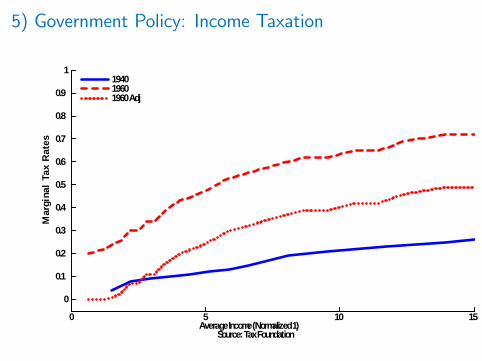
5) Government Policy: Income Taxation

0 5 10 15

0

0.1

0.2

0.3

0.4

0.5

0.6

0.7

0.8

0.9

1

Average Income (Normalized 1)Source: Tax Foundation

Mar

gina

l Ta

x R

ates

194019601960 Adj

II) The Nature of the Co-movement of Ownershipand House Prices: Simple Equilibrium Model

EnvironmentI Two sector model with housingI Agents are heterogeneous in their labor ability ε ∈ [ε, ε], andthe distribution is uniform ε˜U(ε, ε) ≡ f (ε).

I Commodities: c ∈ R+ and h ∈ {0, h} . Renters consumezero housing and homeowners consume a positive amount.

I Preferences (γ > 0):

u(c, h) = c(γ+ h),

I CRS goods sector and housing

C = zcNc ,

H = zhNh.

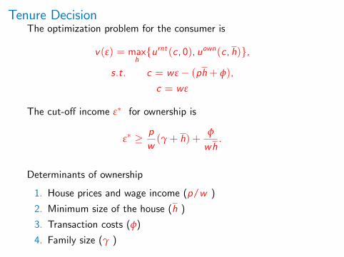
Tenure DecisionThe optimization problem for the consumer is

v(ε) = maxh{urnt (c, 0), uown(c, h)},

s.t. c = w ε− (ph+ φ),

c = w ε

The cut-off income ε∗ for ownership is

ε∗ ≥ pw(γ+ h) +

φ

wh.

Determinants of ownership

1. House prices and wage income (p/w )2. Minimum size of the house (h )

3. Transaction costs (φ)

4. Family size (γ )

Equilibrium Prices

Goods sector:maxNczcNc − wNc ,

w = zg .

Housing sector:maxNhpzhNh − wNh,

p =zczh.

Equilibrium Homeownership

I Connection of key variables necessary to understand theco-movement

HOR =∫ ε

ε∗U(ε, ε)dε =

1ε− ε

[ε−

((γ+ h)zh

+φ

zch

)].

I Increases in the productivity of either sector generatesincreases the homeownership rate, but only one constellationworks. Define

∆w =w ′

w=z ′czc= ∆zc .

∆p =z ′czc

zhz ′h=

∆zc∆zh

.

Co-movementThe co-movement depends on the relative productivity change.

I Symmetric productivity (∆zc = ∆zh):

∆HOR > 0

∆p =∆zc∆zh

= 0

I Asymmetric productivity (∆zc 6= ∆zh ≥ 0):

∆HOR > 0

∆p =∆zc∆zh

> 0

only when ∆zc > ∆z ⇒ ∆w > ∆p

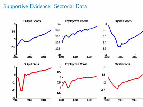
Supportive Evidence: Sectorial Data

1940 1950 19602

2.5

3

3.5

4Output Goods

1940 1950 1960­3

­2

­1

0

1Output Const.

1940 1950 196010

10.2

10.4

10.6

10.8

11Employment Goods

1940 1950 196066.5

77.5

88.5

9Employment Const.

1940 1950 19603

3.2

3.4

3.6

3.8

4Capital Goods

1940 1950 1960­3

­2.5

­2

­1.5

­1Capital Const.

Supportive Evidence: Productivity Differences

1940 1945 1950 1955 1960 19650

0.2

0.4

0.6

0.8

1

1.2

1.4

1.6

1.8

2

GoodsConstruction

III) Quantitative Analysis

Housing Model

I Multi-sector growth model (goods and housing)I Life Cycle Households

I Income risk, and uncertain life expectancyI Choices: Consumption, savings, housing purchase andmortgage choice

I Mortgage Brokers: Provide long-term lending contractsI Government: Progressive income taxation, housing policy, andsocial security

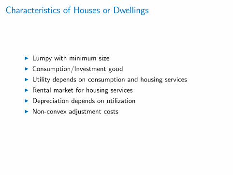
Characteristics of Houses or Dwellings

I Lumpy with minimum sizeI Consumption/Investment goodI Utility depends on consumption and housing servicesI Rental market for housing servicesI Depreciation depends on utilizationI Non-convex adjustment costs

Mapping the Model and the Data (I)

I Preferences:

u(c , d) =[γc−ρ + (1− γ)d−ρ]

− 1−σρ

1− σ

I Technologies:

Yc = zcK 0.3c N0.7c

Yh = zhK0.12h N0.88h

Model Fit: 1935-40

Home Ownership by Age (%)

Data Model1930 1940 1940

25-35 20.0 19.1 13.036-45 48.5 42.1 42.546-55 57.7 51.0 59.256-65 65.1 57.5 69.8Total 48.1 42.7 43.5

Source: US. Census Bureau

Model Predictions 1960: Ownership and Prices

Data 1940 1960 ∆Ownership Rate (%) 42.5 63.5 21.0House Price Index 100 43.0 43.0%

ModelOwnership Rate (%) 43.5 64.5 21.0House Prices 100 140.4 40.4

Model Predictions 1960: Ownership by Age

Model Prediction for Homeownership Rate 1940-60

Data (%) Model (%)Difference Difference

25-35 37.1 32.136-45 26.0 23.846-55 18.5 14.556-65 11.8 15.7Total 21.0 21.0

Source: US. Census Bureau

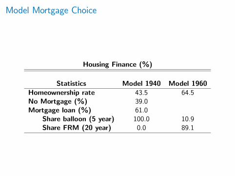
Model Mortgage Choice

Housing Finance (%)

Statistics Model 1940 Model 1960Homeownership rate 43.5 64.5No Mortgage (%) 39.0Mortgage loan (%) 61.0

Share balloon (5 year) 100.0 10.9Share FRM (20 year) 0.0 89.1

The Importance of Productivity

Importance of Relative Productivity Change

Model: 1960 (HR) (ph) ´HR %∆ph

∆zc > ∆zh 64.5 140.2 21.5 40.2∆zc = ∆zh 53.5 106.4 10.2 6.4∆zh = ∆zc 74.7 111.6 31.4 11.6

Decomposition

Contribution Ownership (%) House Prices (%)Demographics 5-8 1-2Income risk 12-57 0-0.51Govn’t Policy 3-4 0-14Housing finance 5-7 1-1.5

Conclusions

I The goal is to understand the driving forces in the postwarhousing boom.

I We use a heterogenous general equilibrium model to measurethe relative importance of prominently mentioned factors.

I The models suggests all factors play a significant roleI House prices: Productivity is essential for house prices, thedemand components account around 5-8

I Ownership: Income, demographics, and governmentintervention in housing finance play are significant