Construction and Validation of Prediction

Models for Number of Changes to

Requirements

Annabella Loconsole & Jurgen Borstler

Department of Computing Science, Umea University, SE-90187 Umea, Sweden{bella,jubo}@cs.umu.se, Phone:+46 90 7866372, Fax:+46 90 7866126

Abstract

In this paper we present a correlational study in which we assess the ability of fivesize measures to predict the number of changes to requirements for a medium sizesoftware project. The study is explorative, i.e. we analyse the data collected for ourmeasures to find out the best predictor of number of changes. To our knowledge,no empirical validation of requirements change measures as predictors has beenperformed in an industrial setting. Based on the data collected from two industrialprojects for five measures of size of requirements (number of actors, use cases, words,lines, and revisions), we have built and evaluated prediction models for number ofchanges to requirements. These models can help project managers to estimate thevolatility of requirements and minimize the risks caused by volatile requirements,like schedule and costs overruns. We performed a cross systems validation. For ourbest model we calculated a pred(0.25)=0.5, which is better than the accuracy ofprediction models like COCOMO. Although our models are likely to have onlylocal validity, the general method for constructing the prediction models could beapplied in any software development company. In an earlier study, we showed thatdecisions solely based on developer perception are unreliable. Predictions models,like the one presented here can help to mitigate that risk.

Key words: Requirement, Prediction Model, Empirical Validation, CorrelationalStudy

1 Introduction

Requirements engineering is an important phase of software development,where the needs of the stakeholders are collected, developed, and documented.Requirements development is a learning rather than a gathering process. As aconsequence, requirements change frequently, even during later stages of the

Preprint submitted to Elsevier Science 20 September 2006

development process. Software requirements that change often are usually saidto be volatile. Studies show that requirements volatility has a high impact onproject performance (Pfahl and Lebsanft, 2000; Stark et al., 1999; Zowghiand Nurmuliani, 2002). However, we cannot expect the requirements to bestable, even when requirements engineering tasks (such as elicitation, analy-sis, specification, and validation) are well performed. It is therefore importantto carefully monitor and control the requirements throughout the software lifecycle. Monitoring requirements volatility usually involves measuring trends orpercentages of changes to requirements (see section 4.2). Anticipating a cer-tain level of volatility project managers can take appropriate actions in orderto decrease project risks.

In this paper, we describe a correlational study with the goal of empiricallyvalidating five measures of requirements size as predictors for the number ofrequirements changes. We built seven prediction models using data collectedfor a medium-size software project developed at BAE Systems Hagglunds AB,Sweden. We then evaluated the accuracy of five models by applying them ona set of data collected for a second project at the same company.

The results show that the best predictors of number of changes are the lengthmeasures: number of lines and words. Other predictors of complexity andfunctionality were found less accurate. The models created can be used on atimely basis to predict volatility trends.

The remaining part of the paper proceeds as follows: section 2 describes theresearch related to empirical validation of measures in general and work re-lated to requirements volatility. In section 3 we briefly summarise our previouscase study, which investigated the relationship between four measures of sizeof use case models and requirements volatility. Section 4 describes the goals,hypotheses, and data collected in the present empirical study. The data anal-ysis and the resulting prediction models are described in section 5. Finally,discussions and conclusions are presented in section 6.

2 Related work

There is little empirical research in the area of requirements volatility. Themajority of the published studies, evaluate the impact of requirements volatil-ity on software projects (Stark et al., 1999; Zowghi and Nurmuliani, 2002), onsoftware products (Henry and Henry, 1993), and defect density (Javed et al.,2004; Malaiya and Denton, 1999).

Many measures related to requirements volatility have been proposed in the

2

literature. Measures to assess requirements stability 1 are presented by Ambri-ola and Gervasi (2000). They showed that requirements stability had a highpredictive value of project risks in a requirements analysis process. Other mea-sures (Costello and Liu, 1995; Henderson-Sellers et al., 2002; Huffman et al.,1998; Hyatt and Rosenberg, 1996; Malaiya and Denton, 1999; Nurmulianiet al., 2004; Raynus, 1999; Stark et al., 1999) concern requirements volatility.In most of the cases, the definition of volatility expresses the changing natureof the requirements (see section 4.2 for further details). A few correlationalstudies are present in the requirements volatility literature (Ambriola and Ger-vasi, 2000; Henry and Henry, 1993; Javed et al., 2004; Loconsole and Borstler,2005; Stark et al., 1999) but, except Loconsole and Borstler (2005), require-ments volatility was chosen as independent variable i.e. as predictor of otherattributes. Henry and Henry (1993) for example, propose measures to predictthe impact of volatility on the software product. Similarly, Stark et al. (1999)present measures to predict the effects of changing requirements on costs andschedule. Javed et al. (2004) present measures of correlation between volatilityand software defects.

The majority of the measures above are designed for well specified and wellwritten requirements, using standardised documentation templates. However,even in the case of well-documented requirements, measures have to be tai-lored towards the particular organisation, because each company has its ownway of documenting requirements. Among those measures, only Ambriola andGervasi (2000) and Loconsole and Borstler (2005) provide an empirical vali-dation. The reason for validating measures is to empirically demonstrate theirpractical utility, i.e. to show that there is a consistent relationship betweenthe measure and an external attribute (Fenton and Pfleeger, 1996; Kitchenhamet al., 1995; Schneidewind, 1992; Zuse, 1997). It is important to ensure thatthe data collected for a certain measure is related to the actual property in-vestigated (the attribute to be measured). Otherwise time and money is spentfor collecting useless data. To our knowledge, only one empirical validation ofrequirements volatility measures has been performed in an industrial setting(Loconsole and Borstler, 2005). In that study we showed a high correlationbetween four measures of size and number of changes to use case models (seesection 3 for further details).

The measures we are interested in are measures that can help to predict thenumber of changes to requirements and this, in turn, can be used to deter-mine volatility. There are no studies on prediction models of requirementschanges. Bush and Finkelstein (2002, 2003) describe a process that could sup-

1 Sometimes, the word stability is used instead of volatility. For instance, a defini-tion of “degree of stability” of requirements is presented in (IEEE830-1998, 1998).Both terms are used conjunctly in (Huffman et al., 1998; Raynus, 1999). In ouropinion, the words are antonyms.

3

port a predictive view of requirements stability. Starting from an initial set ofrequirements, this process helps to create worlds of possible evolutions of re-quirements. They also report on positive results from an industrial case studyvalidating the approach. However, using their process is complex and timeconsuming. Our approach is much simpler and better suited for small andmedium size companies. It is based on use case requirements. Nevertheless,except use case diagrams, the requirements are mainly text based, therefore,it is possible to generalise our results. Further studies are needed to prove this.

3 Background

In an earlier industrial case study (Loconsole and Borstler, 2005), we inves-tigated measures of volatility for a medium size software project. Our goalswere: 1) to empirically validate a set of measures associated with the volatil-ity of requirements documents; and 2) to investigate the correlation betweenperceived and measured volatility. We collected size and change data in ret-rospect for all versions of requirements documents of the software project. Inaddition, we determined the perceived volatility by interviewing stakeholdersof the project.

The spearman correlation coefficient was calculated between each measureof size of requirements documents and the size of changes to requirementsdocuments. Requirements in the project were described in terms of use casesand each requirements document contained one use case model. The size of arequirements document was measured in terms of number of lines, number ofwords, number of use cases, and number of actors.

The data analysis showed a high correlation between each of the size measuresand the total number of changes. This suggests that our measures of size ofrequirements documents are good indicators of the number of changes for usecase based requirements documents. For the second goal, we could not findsignificant correlations between any of our four volatility measures and therating of volatility by the experts. This implies that the developers’ perceptionsof number of changes were not good indicators of requirements volatility forthe project analysed. These results suggest that managers at this companyshould measure their projects because of the risk to take wrong decisionsbased solely on their own and the developers perceptions.

4

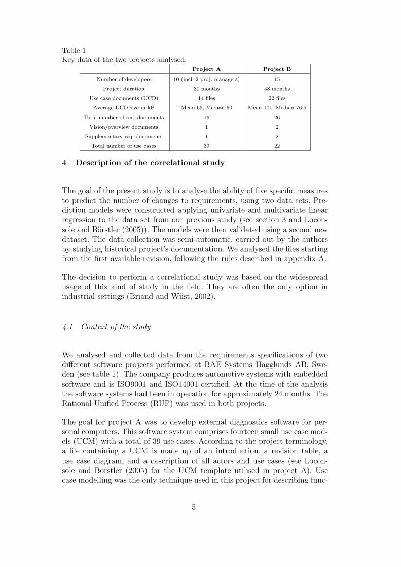
Table 1Key data of the two projects analysed.

Project A Project B

Number of developers 10 (incl. 2 proj. managers) 15

Project duration 30 months 48 months

Use case documents (UCD) 14 files 22 files

Average UCD size in kB Mean 65, Median 60 Mean 101, Median 76.5

Total number of req. documents 16 26

Vision/overview documents 1 2

Supplementary req. documents 1 2

Total number of use cases 39 22

4 Description of the correlational study

The goal of the present study is to analyse the ability of five specific measuresto predict the number of changes to requirements, using two data sets. Pre-diction models were constructed applying univariate and multivariate linearregression to the data set from our previous study (see section 3 and Locon-sole and Borstler (2005)). The models were then validated using a second newdataset. The data collection was semi-automatic, carried out by the authorsby studying historical project’s documentation. We analysed the files startingfrom the first available revision, following the rules described in appendix A.

The decision to perform a correlational study was based on the widespreadusage of this kind of study in the field. They are often the only option inindustrial settings (Briand and Wust, 2002).

4.1 Context of the study

We analysed and collected data from the requirements specifications of twodifferent software projects performed at BAE Systems Hagglunds AB, Swe-den (see table 1). The company produces automotive systems with embeddedsoftware and is ISO9001 and ISO14001 certified. At the time of the analysisthe software systems had been in operation for approximately 24 months. TheRational Unified Process (RUP) was used in both projects.

The goal for project A was to develop external diagnostics software for per-sonal computers. This software system comprises fourteen small use case mod-els (UCM) with a total of 39 use cases. According to the project terminology,a file containing a UCM is made up of an introduction, a revision table, ause case diagram, and a description of all actors and use cases (see Locon-sole and Borstler (2005) for the UCM template utilised in project A). Usecase modelling was the only technique used in this project for describing func-

5

tional requirements. The vision document contained only sketchy, high levelrequirements and was not analysed. Seven non functional requirements weredescribed in one additional file.

Project B developed an information and control system for the vehicles con-structed by the company. This software system comprises 22 use cases andother non functional requirements described in two documents. Accordingto the project terminology, a use case description contains the following sec-tions: overview, revision history, references, description, state-diagram, normalflow, alternative flows, special requirements, start conditions, end conditions,and extension points. The actors of this system were described in a higherlevel requirements specification document called “use case summary”. In theseprojects, we consider use cases as requirements 2 .

As can be observed from table 1, the documentation for projects A and B didnot match completely, even though the projects were developed in the samecompany. No developer worked on both systems. The objects chosen for thestudy were the requirements documents of the two projects described above.In project A we analysed fourteen files, each containing a very small use casemodel. In project B we analysed twenty-two files, each containing one use case.Other documentation, used to understand the projects A and B, were visiondocuments (the top level requirements specification), the use case summary(where we counted the actors), project plans, iteration plans, and test plans.

4.2 Dependent variables

Our goal was to investigate the relationship between requirements size mea-sures and requirements volatility. We therefore had to choose a suitable andpractical measure of volatility as the dependent variable of our study. Theo-retical definitions of requirements volatility are presented in (Baumert andMcWhinney, 1992; Nurmuliani et al., 2004; Raynus, 1999; Rosenberg andHyatt, 1996), while operational definitions can be found in (Baumert andMcWhinney, 1992; Chrissis et al., 2003; Hyatt and Rosenberg, 1996; Locon-sole and Borstler, 2005; Nurmuliani et al., 2004; Raynus, 1999; Stark et al.,1999). Baumert and McWhinney (1992), suggest to measure source and stateof change, while Nurmuliani et al. (2004) take into consideration the source ofchange in their theoretical definition of volatility. Except these two cases, alldefinitions have several things in common:

(1) They express the changing nature of requirements during the softwaredevelopment.

2 We are aware of the fact that some researchers do not consider use cases asrequirements (Ham, 1998; Lau, 2004; Schneider and Winters, 1998; Young, 2004).

6

(2) They focus on the amount of changes (additions, deletions, and modifi-cations) to requirements.

(3) They do not consider the cause of change and the semantics of a change,i.e. in what way a change impacts development.

That means that volatility is treated as a quantitative measure. Likewise, wedefine requirements volatility as the amount of changes to a requirements doc-ument over time, and will measure it as the number of changes (NCHANGE)to a requirements document. There is one difference between our operationaldefinition of volatility and the ones above. We look at volatility document bydocument instead of threating all requirements as one set. This enables us toidentify different degrees of volatility within the whole set of requirements.

NCHANGE is a direct measure which is necessary in order to calculate otherimportant indirect measures like change density and frequency of change. Re-quirements change density can easily be computed by dividing NCHANGE byrequirements size. Frequency of change is calculated by applying NCHANGEwithin specific time intervals. In this way we can also identify volatility trends.

Please note that we do not do any cause-effect or impact analyses of indi-vidual changes to requirements. Such qualitative analyses would require othertypes of measures, like for example the type of a change or the number ofartefacts affected by a change. Such data is usually not available early on inthe development. The downstream artefacts that could possibly be affectedby a change (design and code for example) are not available yet.

Our dependent variable NCHANGE has been determined by comparing ver-sions of requirements documents by means of a tool and counting the changesfrom one version of a document to the next. A detailed description of thecounting rules can be found in appendix A.

4.3 Independent variables

The choice of the independent variables depends on the entity and the size ofthe systems measured. Because the projects under analysis are different fromeach other, it is necessary to select general measures that can be applied inboth project contexts. This is also necessary to increase general applicabilityof results.

The entities analysed in the two projects were requirements documents. Inproject A we analysed fourteen files each containing a small use case model.In project B we analysed twenty-two files, each containing one use case. In-tuitively, the larger the document the more changes there are. Therefore, webelieve that the size of requirements is the most influential factor affecting

7

volatility. The size measures “number of actors interacting with the use casesdescribed in the file” (NACTOR), “number of lines per file” (NLINE), “num-ber of words per file” (NWORD), “number of use cases per file” (NUC), and“number of revisions per file” (NREVISION) are the independent variableschosen for this study. As suggested by Fenton and Pfleeger (1996), size can beseen as composed of length, functionality, and complexity. In our case, NLINEand NWORD are measures of length, NACTOR and NREVISION are mea-sures of complexity, and NUC is a measure of functionality. These measuresare quite intuitive. The NLINE and NWORD are simply a count of lines andwords of the files analysed and were calculated by the authors using a com-puterised tool. NACTOR is a count of the number of actors interacting withthe use cases described in each file analysed. NREVISION is a count of therevisions for each file. A revision is a version of a file with a unique identifier.In our previous study (see section 3) we did not analyse the correlation ofNREVISION with number of changes.

The independent variables are defined as measures of size. The size of a re-quirement document can be computed at varying levels of granularity, becausethe requirements documents are organised hierarchically. We did not collectmeasures at higher or lower abstraction level, because we considered thoserequirements as either too vague or too close to the design level.

Selecting NLINE as independent variable might seem controversial. Like linesof code (LOC) as a size measure for program size, NLINE depends on thelanguage used and formatting style. As pointed out by Armour (2004), whatwe actually want to measure is how much knowledge there is in our system orfile. Unfortunately, there is not yet an empirical way to measure knowledge. Apossible choice for the independent variable could be use case points (UCPs)(Schneider and Winters, 1998). Effort estimation models based on UCP havebeen investigated by Anda (2002). However, UCPs are not generally appli-cable. The definition of UCPs is based on a classification of use cases anda number of environmental factors (similar to the cost drivers in COCOMO(Boehm, 1981)). This information was not available for our projects. Theclassification of use cases is a subjective activity, therefore it is not possibleto collect UCPs automatically.

Other possible independent variables could be the total number of require-ments, the number of requirements added and deleted, or the number of initialand final requirements. These are system measures, i.e. we need to have sev-eral systems to be able to count these measures. Furthermore, these measureswould make it necessary to exactly define what a single atomic requirementis, otherwise it cannot be counted reliably. Other measures like “number of as-sociations between use cases”, “number of steps in scenarios”, were discardedbecause they were not readily available. The measures chosen for this studyare not necessarily the most appropriate for all projects but were a suitable

8

choice for the projects analysed.

4.4 Hypothesis

The hypothesis of the study is the following: the size measures NACTOR,NUC, NWORD, NLINE, and NREVISION are good predictors of number ofrequirements changes. Our hypothesis is built on the idea that larger require-ments are affected by changes more than smaller ones, because they containmore information. The relationship between number of changes and our fivemeasures of size of a requirements document could be causal. However, in thisstudy we only looked at whether a relationship exists, and whether our mea-sures of size can be used as predictors of number of changes to requirements.The study does not make any claims with respect to causality which can beproven only by performing controlled experiments. In industrial environmentsit is usually hard to perform controlled experiment. For real projects, it is dif-ficult to control variables, such as project length, the experience of customersand developers in specifying requirements, the techniques used to collect anddocument requirements, and the company’s maturity (in requirements andsoftware processes in general). In academic environments, on the other hand,the small size of the projects does not usually allow to check for changes torequirements (Loconsole and Borstler, 2004).

5 Analysis results

As described in section 3, in our previous study we found a strong correlationbetween four of the five size measures introduced in section 4.3 with totalnumber of changes (Loconsole and Borstler, 2005). Furthermore, the scatterplots of our measures versus number of changes show approximately a linearcorrelation (see figure 1 and 2), especially for the length measures. Based onthose results, we have analysed the ability of our measures to predict thenumber of changes to requirements. For this analysis we applied univariateand multivariate linear regression which is suggested to predict interval andratio scale dependent variables (Briand and Wust, 2002).

The data analysis is obtained by following the procedure suggested by Briandand Wust (2002); Briand et al. (2000), which is also described in statisti-cal books such as Draper and Smith (1966). We start with the descriptivestatistics performed on data sets A and B (section 5.1). The principal compo-nent analysis (5.2), univariate analysis (5.3), multivariate regression analysis(5.4), sanity tests on the regression models (5.5), and evaluation of goodnessof fit (5.6) were performed only on data set A. In section 5.7 we evaluate the

9

prediction models by applying them on data set B.

5.1 Descriptive statistics

Table 2 shows the descriptive statistics for data sets A and B. The columnsSE Mean, StDev, and IQR state respectively mean standard error, standarddeviation, and inter quartile range.

In both data sets, the mean NCHANGE is larger than the median 3 . Thestandard deviation in data set B is higher than the mean, this is due to someoutliers. Furthermore, the mean is more than two times higher than the meanin data set A. This implies that the prediction models, built based on dataset A, will probably predict low numbers of changes for data set B.

NC

HA

NG

E

900600300 642 15010050

1000

750

500

250

0

864

1000

750

500

250

0321

NWORD NUC NLINE

NREVISION NACTOR

13353

953

328

763

238

808

472

263

388

279

117

347

220

13353

953

328

763

238

808

472

263

388

279

117

347

220

13353

953

328

763

238

808

472

263

388

279

117

347

220

13353

953

328

763

238

808

472

263

388

279

117

347

220

13353

953

328

763

238

808

472

263

388

279

117

347

220

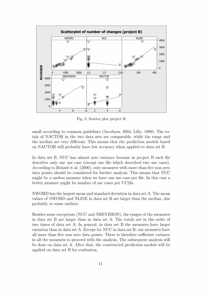
Scatterplot of number of changes (project A)

Fig. 1. Scatter plot project A

NACTOR, NUC, and NREVISION have relatively low means, standard devia-tions, and variances in both data sets. Low variance measures do not differenti-ate entities very well, therefore they are not likely to be useful predictors. Thelow variance of NACTOR and NUC is due to the fact that the requirementsdocuments under analysis contain very few use cases and actors. However,NACTOR and NUC can be expected to be low, since UCMs should be kept

3 Extremely high or low measurements will not affect the median as much as theyaffect the mean. Thus, when we deal with skewed populations we may prefer themedian to the mean to espress central tendency (Zar, 1999).

10

NC

HA

NG

E

200010000 2,01,51,0 4002000

4000

3000

2000

1000

0

1284

4000

3000

2000

1000

0

642

NWORD NUC NLINE

NREVISION NACTOR

170172377456362490

213407

239

1540

227375

115280

1038

383

1207

3715

2587

587

12231526

170172377456362490213407239

1540

227375115280

1038

383

1207

3715

2587

587

12231526

170172377456362490

213407

239

1540

227375

115280

1038

383

1207

3715

2587

587

12231526

170172377456362490

213407

239

1540

227375115

280

1038

383

1207

3715

2587

587

12231526

170172377456362490213

407239

1540

227375115280

1038

383

1207

3715

2587

587

12231526

Scatterplot of number of changes (project B)

Fig. 2. Scatter plot project B

small according to common guidelines (Jacobson, 2004; Lilly, 1999). The to-tals of NACTOR in the two data sets are comparable, while the range andthe median are very different. This means that the prediction models basedon NACTOR will probably have low accuracy when applied to data set B.

In data set B, NUC has almost zero variance because in project B each filedescribes only one use case (except one file which described two use cases).According to Briand et al. (2000), only measures with more than five non zerodata points should be considered for further analysis. This means that NUCmight be a useless measure when we have one use case per file. In this case abetter measure might be number of use cases per UCMs.

NWORD has the largest mean and standard deviation in data set A. The meanvalues of NWORD and NLINE in data set B are larger than the median, dueprobably to some outliers.

Besides some exceptions (NUC and NREVISION), the ranges of the measuresin data set B are larger than in data set A. The totals are in the order oftwo times of data set A. In general, in data set B the measures have largervariation than in data set A. Except for NUC in data set B, our measures haveall more than five non zero data points. There is therefore sufficient variancein all the measures to proceed with the analysis. The subsequent analysis willbe done on data set A. After that, the constructed prediction models will beapplied on data set B for evaluation.

11

Table 2Descriptive statistics for data sets A and B.

Data set Measures Range Total Mean SE Mean StDev Variance Median IQR

A(14 files)

NCHANGE 900 5360 382.9 73.3 274.1 75138.9 303.5 345

NACTOR 2 5 1.5 0.174 0.65 0.423 1 1

NUC 5 39 2.786 0.447 1.672 2.797 3 2.25

NLINE 105 1436 102.57 8.35 31.24 975.96 100.5 52.5

NWORD 852 8771 626.5 73.9 276.4 76375.5 663.5 492.8

NREVISION 5 89 6.357 0.44 1.646 2.709 6.5 3.25

B(22 files)

NCHANGE 3600 17689 804 191 895 801152 395 975

NACTOR 5 6 3.182 0.276 1.296 1.68 4 2

NUC 1 23 1.0455 0.0455 0.2132 0.0455 1 0

NLINE 378 2848 129.5 18.7 87.9 7720.1 109 97

NWORD 2379 16831 765 123 578 333794 606 822

NREVISION 7 64 2.909 0.354 1.659 2.753 2 1

Table 3Rotated components for data set A.

Measures PC1 PC2 PC3 PC4 PC5

Eigenvalue 3.3979 0.7848 0.6296 0.1732 0.0145

Percent 68 15.7 12.6 0.35 0.03

Cumulative 68 83.7 96.2 99.7 100

NACTOR 0.308 -0.183 -0.929 0.091 -0.003

NLINE 0.807 -0.290 -0.385 0.321 -0.115

NUC 0.496 -0.328 -0.112 0.796 -0.005

NREVISION 0.128 -0.954 -0.175 0.207 -0.008

NWORD 0.92 -0.051 -0.257 0.285 0.055

5.2 Principal component analysis

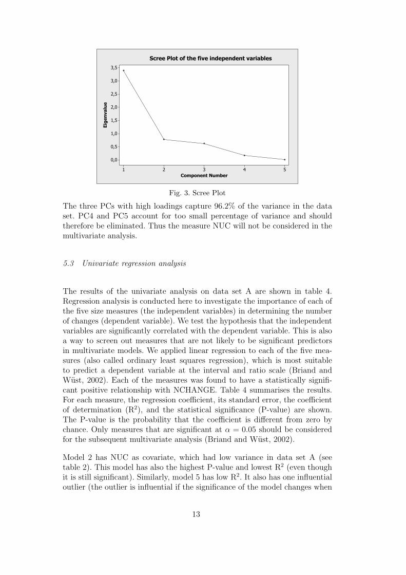
Principal component (PC) analysis is performed in order to form a smallernumber of uncorrelated variables, by selecting the independent variables withhigh loadings. For a set of n measures, there are at most n orthogonal PCs,which are calculated in decreasing order of variance they explain in the dataset. Table 3 shows the results of the varimax rotation performed on data setA. This technique allows to identify a clearer pattern of loadings. For eachPC, we provide its eigenvalue, the variance of the data set explained by thePC (in percent), and the cumulative variance. Absolute values above 0.7 areset in boldface.

As we can see in table 3, NLINE and NWORD get high factor loadings in PC1.They express the same orthogonal dimension, i.e. the length of requirementsdocuments. NREVISION, NACTOR, and NUC get high loadings in PC2,PC3, and PC4, respectively. PC2 and PC3 express complexity, while PC4expresses functionality dimensions. Among the five PCs shown in the table,three of them show sufficient variance, as shown by the scree plot in figure 3.

12

Component Number

Eige

nva

lue

54321

3,5

3,0

2,5

2,0

1,5

1,0

0,5

0,0

Scree Plot of the five independent variables

Fig. 3. Scree Plot

The three PCs with high loadings capture 96.2% of the variance in the dataset. PC4 and PC5 account for too small percentage of variance and shouldtherefore be eliminated. Thus the measure NUC will not be considered in themultivariate analysis.

5.3 Univariate regression analysis

The results of the univariate analysis on data set A are shown in table 4.Regression analysis is conducted here to investigate the importance of each ofthe five size measures (the independent variables) in determining the numberof changes (dependent variable). We test the hypothesis that the independentvariables are significantly correlated with the dependent variable. This is alsoa way to screen out measures that are not likely to be significant predictorsin multivariate models. We applied linear regression to each of the five mea-sures (also called ordinary least squares regression), which is most suitableto predict a dependent variable at the interval and ratio scale (Briand andWust, 2002). Each of the measures was found to have a statistically signifi-cant positive relationship with NCHANGE. Table 4 summarises the results.For each measure, the regression coefficient, its standard error, the coefficientof determination (R2), and the statistical significance (P-value) are shown.The P-value is the probability that the coefficient is different from zero bychance. Only measures that are significant at α = 0.05 should be consideredfor the subsequent multivariate analysis (Briand and Wust, 2002).

Model 2 has NUC as covariate, which had low variance in data set A (seetable 2). This model has also the highest P-value and lowest R2 (even thoughit is still significant). Similarly, model 5 has low R2. It also has one influentialoutlier (the outlier is influential if the significance of the model changes when

13

Table 4Univariate regression analysis for data set A (α = 0.05).

Models Measure Coeff. Std. Err. P-value R2

1 NACTOR 314.18 81.08 0.002 55.6

2 NUC 99.34 37.64 0.022 36.7

3 NLINE 7.858 1.127 0.000 80.2

4 NWORD 0.7818 0.1762 0.001 62.1

5 NREVISION 97.62 35.68 0.019 40.5

performing the test without the outlier). Therefore, this model will be evalu-ated without the outlier (as suggested by Briand and Wust (2002)). A deeperanalysis of outliers and model checking is done in section 5.5.

Observing table 4, the R2 value of model 3 is 80.2. This means that model3 explains 80.2% of the variation in number of changes. Similarly we caninterpret the results for the other models. The goal of this test was to determineif each measure is a useful predictor of number of changes. Although themeasures are all significant, NACTOR, NLINE, and NWORD seem to bebetter predictors than NUC and NREVISION.

5.4 Multivariate regression analysis

In this section we present the construction of prediction models built on dataset A, with the goal of accurately predicting the number of changes to require-ments. Because this study is exploratory, we do not know which independentvariables should be included in the prediction models. Usually, a stepwise se-lection process is used (Briand and Wust, 2002; Levine et al., 2001; Zar, 1999).A common method to reduce the number of independent variables is to usethe results from the principal components analysis as filter, selecting only thevariables with high loadings in the significant PCs. In our case only threePCs had sufficient variance, and this lead us to discard the measure NUC.We applied the multivariate linear regression starting with four variables. Thestatistics tool used for the analysis (Minitab) gives the possibility to check forcollinearity. As expected, NLINE and NWORD were found collinear, thereforewe continued the statistical analysis excluding NLINE.

Only two models with two covariates were found significant (see table 5).Both models have NWORD as one of the covariates. Model 6 (NWORD andNREVISION) had one influential outlier. Therefore, in the following sections,it will be evaluated without the outlier (as suggested by Briand and Wust(2002)). A deeper analysis of outliers and model checking is done in section 5.5.We discarded the models with a P-value higher than 0.05 in the t-test.

14

Table 5Multivariate regression models for data set A.

Models Measures Coeff. Std. Err. P-value R2

6 NWORD 0.6148 0.1239 0.001 82.8

NREVISION 64.39 21.2 0.013

Intercept -444.7 137.9 0.009

7 NACTOR 187.19 75.4 0.030 75.7

NWORD 0.5362 0.1775 0.012

Intercept -233.9 112.6 0.062

5.5 Sanity tests on the regression models

One of the threats to conclusion validity is the violation of assumptions ofstatistical tests. To be valid, the models have to satisfy some hypothesis onthe residuals. We followed the tests suggested in (Levine et al., 2001). Thesanity checks were performed on five univariate models and two multivariatemodels. See figure 4 for an example of the plots generated for the analysis ofthe residuals.

Residual

Per

cen

t

5002500-250-500

99

90

50

10

1

Fitted Value

Res

idu

al

600400200

600

400

200

0

-200

Residual

Freq

uen

cy

5004003002001000-100-200

4,8

3,6

2,4

1,2

0,0

Observation Order

Res

idu

al

1413121110987654321

600

400

200

0

-200

Normal Probability Plot of the Residuals Residuals Versus the Fitted Values

Histogram of the Residuals Residuals Versus the Order of the Data

Residual Plots for number of changes: NUC

Fig. 4. Residuals analysis for model 2, NUC

The results of the model checking is listed below.

(1) Linear relationship between response and predictors. The ”lack-of-fit-test”,did not show any evidence of lack of fit for p >= 0.1 in any of the sevenmodels.

(2) Homogeneity of variance (the residuals have constant variance). The resid-uals versus fits plot did not reveal patterns in any case.

15

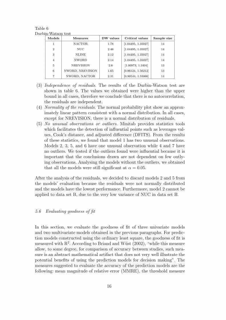
Table 6Durbin-Watson test

Models Measures DW values Critical values Sample size

1 NACTOR 1.78 [1.04495, 1.35027] 14

2 NUC 2.46 [1.04495, 1.35027] 14

3 NLINE 2.12 [1.04495, 1.35027] 14

4 NWORD 2.14 [1.04495, 1.35027] 14

5 NREVISION 2.6 [1.00973, 1.3404] 13

6 NWORD, NREVISION 1.65 [0.86124, 1.56212] 13

7 NWORD, NACTOR 2.31 [0.90544, 1.55066] 14

(3) Independence of residuals. The results of the Durbin-Watson test areshown in table 6. The values we obtained were higher than the upperbound in all cases, therefore we conclude that there is no autocorrelation,the residuals are independent.

(4) Normality of the residuals. The normal probability plot show an approx-imately linear pattern consistent with a normal distribution. In all cases,except for NREVISION, there is a normal distribution of residuals.

(5) No unusual observations or outliers. Minitab provides statistics toolswhich facilitates the detection of influential points such as leverages val-ues, Cook’s distance, and adjusted difference (DFITS). From the resultsof these statistics, we found that model 1 has two unusual observations.Models 2, 3, 5, and 6 have one unusual observation while 4 and 7 haveno outliers. We tested if the outliers found were influential because it isimportant that the conclusions drawn are not dependent on few outly-ing observations. Analysing the models without the outliers, we obtainedthat all the models were still significant at α = 0.05.

After the analysis of the residuals, we decided to discard models 2 and 5 fromthe models’ evaluation because the residuals were not normally distributedand the models have the lowest performance. Furthermore, model 2 cannot beapplied to data set B, due to the very low variance of NUC in data set B.

5.6 Evaluating goodness of fit

In this section, we evaluate the goodness of fit of three univariate modelsand two multivariate models obtained in the previous paragraphs. For predic-tion models constructed using the ordinary least square, the goodness of fit ismeasured with R2. According to Briand and Wust (2002), “while this measureallow, to some degree, for comparison of accuracy between studies, such mea-sure is an abstract mathematical artifact that does not very well illustrate thepotential benefits of using the prediction models for decision making”. Themeasures suggested to evaluate the accuracy of the prediction models are thefollowing: mean magnitude of relative error (MMRE), the threshold measure

16

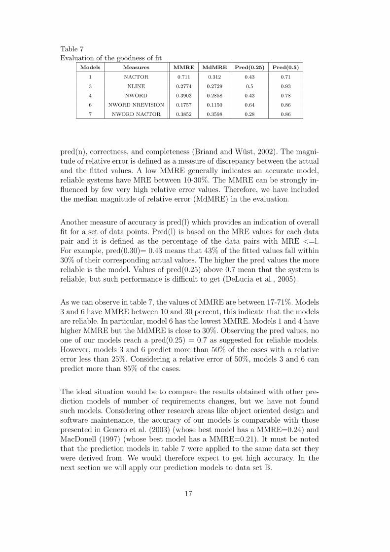
Table 7Evaluation of the goodness of fit

Models Measures MMRE MdMRE Pred(0.25) Pred(0.5)

1 NACTOR 0.711 0.312 0.43 0.71

3 NLINE 0.2774 0.2729 0.5 0.93

4 NWORD 0.3903 0.2858 0.43 0.78

6 NWORD NREVISION 0.1757 0.1150 0.64 0.86

7 NWORD NACTOR 0.3852 0.3598 0.28 0.86

pred(n), correctness, and completeness (Briand and Wust, 2002). The magni-tude of relative error is defined as a measure of discrepancy between the actualand the fitted values. A low MMRE generally indicates an accurate model,reliable systems have MRE between 10-30%. The MMRE can be strongly in-fluenced by few very high relative error values. Therefore, we have includedthe median magnitude of relative error (MdMRE) in the evaluation.

Another measure of accuracy is pred(l) which provides an indication of overallfit for a set of data points. Pred(l) is based on the MRE values for each datapair and it is defined as the percentage of the data pairs with MRE <=l.For example, pred(0.30)= 0.43 means that 43% of the fitted values fall within30% of their corresponding actual values. The higher the pred values the morereliable is the model. Values of pred(0.25) above 0.7 mean that the system isreliable, but such performance is difficult to get (DeLucia et al., 2005).

As we can observe in table 7, the values of MMRE are between 17-71%. Models3 and 6 have MMRE between 10 and 30 percent, this indicate that the modelsare reliable. In particular, model 6 has the lowest MMRE. Models 1 and 4 havehigher MMRE but the MdMRE is close to 30%. Observing the pred values, noone of our models reach a pred(0.25) = 0.7 as suggested for reliable models.However, models 3 and 6 predict more than 50% of the cases with a relativeerror less than 25%. Considering a relative error of 50%, models 3 and 6 canpredict more than 85% of the cases.

The ideal situation would be to compare the results obtained with other pre-diction models of number of requirements changes, but we have not foundsuch models. Considering other research areas like object oriented design andsoftware maintenance, the accuracy of our models is comparable with thosepresented in Genero et al. (2003) (whose best model has a MMRE=0.24) andMacDonell (1997) (whose best model has a MMRE=0.21). It must be notedthat the prediction models in table 7 were applied to the same data set theywere derived from. We would therefore expect to get high accuracy. In thenext section we will apply our prediction models to data set B.

17

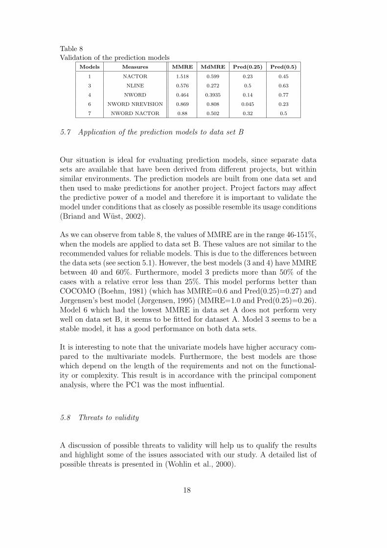
Table 8Validation of the prediction models

Models Measures MMRE MdMRE Pred(0.25) Pred(0.5)

1 NACTOR 1.518 0.599 0.23 0.45

3 NLINE 0.576 0.272 0.5 0.63

4 NWORD 0.464 0.3935 0.14 0.77

6 NWORD NREVISION 0.869 0.808 0.045 0.23

7 NWORD NACTOR 0.88 0.502 0.32 0.5

5.7 Application of the prediction models to data set B

Our situation is ideal for evaluating prediction models, since separate datasets are available that have been derived from different projects, but withinsimilar environments. The prediction models are built from one data set andthen used to make predictions for another project. Project factors may affectthe predictive power of a model and therefore it is important to validate themodel under conditions that as closely as possible resemble its usage conditions(Briand and Wust, 2002).

As we can observe from table 8, the values of MMRE are in the range 46-151%,when the models are applied to data set B. These values are not similar to therecommended values for reliable models. This is due to the differences betweenthe data sets (see section 5.1). However, the best models (3 and 4) have MMREbetween 40 and 60%. Furthermore, model 3 predicts more than 50% of thecases with a relative error less than 25%. This model performs better thanCOCOMO (Boehm, 1981) (which has MMRE=0.6 and Pred(0.25)=0.27) andJørgensen’s best model (Jørgensen, 1995) (MMRE=1.0 and Pred(0.25)=0.26).Model 6 which had the lowest MMRE in data set A does not perform verywell on data set B, it seems to be fitted for dataset A. Model 3 seems to be astable model, it has a good performance on both data sets.

It is interesting to note that the univariate models have higher accuracy com-pared to the multivariate models. Furthermore, the best models are thosewhich depend on the length of the requirements and not on the functional-ity or complexity. This result is in accordance with the principal componentanalysis, where the PC1 was the most influential.

5.8 Threats to validity

A discussion of possible threats to validity will help us to qualify the resultsand highlight some of the issues associated with our study. A detailed list ofpossible threats is presented in (Wohlin et al., 2000).

18

Conclusion validity. One issue that could affect the conclusion validity is therelative small size of the sample data. Concerning data quality, the data forNLINE and NWORD have been collected using a computerised tool and aretherefore reliable. The data collection for NCHANGE, NUC, NACTOR, andNREVISION involved human judgment. However, we have defined measure-ment rules to keep the judgment as objective as possible (see appendix A).Furthermore, the measurement rules have been tested; three subjects haveindependently applied the rules on two versions of a requirement documentobtaining the same results. Finally, because the study has been done in ret-rospect, there is a risk that the data is imprecise, e.g., that the available files(use cases models and use cases) are incomplete. The risk of imprecise datais present even when practitioners capture data when they work. For retro-spective studies this risk is even higher. However, this threat is minimal, therecords were complete, the version handling system had no dangling referencesto missing documents.

Construct validity. The construct validity is the degree to which the variablesare accurately measured by the measurement instruments used in the study.The construct validity of the measures used for the independent and dependentvariables, is ensured by the theoretical validation performed in (Loconsole andBorstler, 2003).

External validity. Our threats to external validity are minimal because thestudy was performed in an industrial environment, therefore the materialsused, and the projects themselves were real. Other factors that may affectthe external validity of this study could be the project length, the experienceof customers and developers in specifying requirements, the techniques usedto collect and document requirements, and the company’s maturity (in re-quirements and software processes). The projects were developed in the samecompany and used (approximately) the same processes, but everything elsewas different: size, personnel, and type of project. That means, we can assumethat the models are valid for a relatively large class of projects.

Internal validity. The study described here is a correlational study. We haveshown that all measures are significantly correlated to number of requirementschanges. However, this relationship does not imply a causal relationship. Onlya controlled experiment, where the measures would be varied in a controlledmanner (and the other factors would be held constant), could demonstratecausality, as we have discussed in section 4.4. One threat to internal valid-ity is the potential inaccuracy of collected data on changes to requirements.Change requests were not available. Actual changes to requirements docu-ments were determined by comparing all revisions of the requirements docu-ments analysed. Rules of measurements on how to count changes were defined(see appendix A). However, we had access to and analysed all revisions of therequirements documents analysed. Version and configuration management is

19

handled seriously at the company. All records were complete (see conclusionvalidity).

6 Discussions and conclusions

In this paper, we have described a correlational study on number of require-ments changes performed at BAE Systems Hagglunds AB, Sweden. We col-lected and analysed data of two historical projects in the company for fivemeasures of size (NUC, NACTOR, NLINE, NWORD, NREVISION). Apply-ing univariate and multivariate regression analysis, we built prediction modelsusing data collected on a medium size software project. We then evaluatedthe models accuracy by applying the models on a set of data collected on asecond, slightly larger, project developed at the same company. Our predictionmodels receive as input data for several measures of size for files describingsoftware requirements. The models produce a number as output: the totalnumber of changes to the requirements document. The dependent variabledoes not measure volatility directly. However, by applying the measure withinspecific time intervals, we can identify volatility trends. From an analysis ofthe volatility trends, project managers can identify critical requirements andallocate resources for analysing reasons for their volatility. In this way theycan minimise the risks of schedule and cost overruns.

Our hypothesis was: the size measures NACTOR, NUC, NWORD, NLINE,and NREVISION are good predictors of number of requirements changes.The data analsys showed that all measures have a positive significant rela-tionship to NCHANGE. The measures are accurate predictors, except NUCand NREVISION that were associated to a low coefficient of determination.The accuracy of the measures as predictors is also shown by the low valuesof MMREs and high values of pred (see table 7). Looking at the coefficientof determination of the univariate models, the best predictor seems to beNLINE, followed by NWORD, NACTOR, NREVISION, and NUC. Similarresults were obtained by measuring the MMREs (see table 7). The multivari-ate model 6, which combine the covariates NWORD and NREVISION, showsthe best performance on data set A. It has the highest coefficient of deter-mination, lowest MMRE, and highest Pred(0.25), but has weak performanceon data set B. This may be due to the differences between the two data setsespecially because NREVISION had different means in the two data sets (seetable 2). When applying the models on data set B, NLINE was the best predic-tor, followed by NWORD, the multivariate model with coovariates NWORDand NACTOR, and the univariate model NACTOR. The predictive ability ofNLINE is comparable to those of known models such as COCOMO (Boehm,1981). It is interesting to note that the best models are those which dependonly on the length of the requirements documents and not on the functional-

20

ity or complexity. This result is in accordance with the principal componentanalysis, where the PC1, associated to the length, was the most influential.

Our models predict the number of changes to a certain requirements docu-ment by using different measures of size of requirements document as input.The problem of predicting number of requirements changes then, becomes aproblem of estimating the size of a requirement document. How can we foreseethat the size of a requirement will increase? If the size is small, the number ofpredicted changes will be small. Given a certain size, our models predict thenumber of changes for that size. When the size changes the models have to beapplied again. Based on these findings, we suggest the following approach forusing the prediction models:

1. Collect data on a current project (NUC, NACTOR, NLINE, NWORD,NREVISION, and NCHANGE).

2. Predict the number of changes in the current project using one of the modelsdescribed earlier, for instance model 3. This particular model would receivevalues of NLINE as input and produce a predicted number of changes asoutput.

3. Compare the actual with the predicted number of changes. If the actualnumber is equal or higher than the predicted number of changes, theremay be no more changes. Alternatively, the requirements document is anoutlier and we need to control that document and eventually redesign it. Ifthe actual number is less than the predicted number of changes, we haveto expect more changes to that requirements document.

Our results suggest that variation in size of requirements specifications implyvariation of number of changes. For a deeper analysis of volatility it is sug-gested to investigate qualitative aspects such as why the changes occur, howcritical the changes are, the type and phase where the changes occur. Inves-tigating many qualitative aspects on many requirements documents is expen-sive, subjective, and not feasible. However, studying the impact of a changemight help to “classify” changes and to identify the most critical changes. Ina qualitative analysis, we would care only about important changes since allothers will not affect the project much. With our prediction models we canquantify the “instability” of requirements in order to identify the critical ones.When the critical requirements are identified, we can perform a deeper analysisof the changes in order to figure out the problems with the requirement.

Although our approach currently uses use case based requirements, the definedmeasures are quite general and can therefore be used for all use case documentswritten in textual form. Furthermore, the measures NLINE and NWORD canbe applied to any kind of requirement written in textual form. Our approach ofusing counts is simple, effective, easily interpreted and completely automated.

21

We believe it is possible to develop prediction systems based upon simplemeasures such as ours. The reason for our confidence is that the correlationalstudy presented here is based on two different industrial projects. Although theexact nature of the prediction systems will vary from company to company,the underlying principle is the same. That is, developers can collect simplemeasures derived from requirements documents, and build effective predictionsystems using techniques like linear regression analysis. Models must howeverbe calibrated to suit different environments (MacDonell, 1997).

We plan to apply the models in larger projects in the same company and inother companies. The study described in this paper needs to be replicated ina variety of environments and systems in order to build a body of knowledgein the area.

A Measurement rules

In this section, we describe the rules we adopted for measuring the require-ments documents of the two analysed projects. For this study we consideredfiles as units of requirements documents. We had full access to the repositoryof the projects and retrieved all existing revisions of all files analysed from thestart of the projects until the point in time of the analysis.

The measure NCHANGE was obtained by counting the number of changesto a unit of requirement document. The size of change is usually dependenton the effort spent for the change or the number of artifacts impacted bythe change. Unfortunately, this information was not available in the currentprojects. Therefore, the size of change was estimated by the authors. We com-pared two successive versions of a file using the “track changes: compare doc-uments” tool in MS Word. Each word added or deleted was considered asone change, while each word substituted was considered as two changes (onedeletion plus one addition). Furthermore, adding a picture, resizing, addinga frame, adding or deleting a detail in a picture were all considered as onechange. Intuitively, adding a picture should be considered a bigger changecompared to resizing it. However, if changes are made in the pictures theseare usually mirrowed with changes in the text.

Exceptions to these rules were the following. We did not count addition ordeletion of empty space, empty lines added or deleted, page breaks or tabswithout text. Automatic changes like the date in the headers and the filenamein the footers were not considered changes. If a section was inserted or deletedand the successive section’s numbers were changed, they were not consideredas changes. The same change repeated many times in different paragraphswas considered as many changes. There were changes like a substitution of a

22

newline where a word appears in red. We did not considered these words aschanged.

References

V. Ambriola and V. Gervasi. Process metrics for requirements analysis. InProc. of the 7th European Workshop on Software Process Technology, pages90–95, February 2000.

B. Anda. Comparing effort estimates based on use case points with expertestimates. In Empirical Assessment in Software Engineering (EASE), Keele,UK, 2002. -.

P.G. Armour. Beware of counting LOC. Communications of the ACM, 47(3):21–24, 2004.

J.H. Baumert and M.S. McWhinney. Software Measures and the CapabilityMaturity Model. Technical Report CMU/SEI-92-TR-025, Pittsburgh, July1992.

B.W. Boehm. Software engineering economics. Prentice Hall PTR, UpperSaddle River, NJ, USA, 1981. ISBN 0138221227.

L.C. Briand and J. Wust. Advances in computers, chapter: Empirical studiesof quality models in object-oriented systems. Academic Press, INC, USA,2002. ISBN 0065-2458.

L.C. Briand, J. Wust, J.W. Daly, and D.V. Porter. Exploring the relationshipsbetween design measures and software quality in object-oriented systems.Journal of Systems and Software, 51(3):245–273, 2000.

D. Bush and A. Finkelstein. Environmental scenarios and requirements stabil-ity. In IWPSE ’02: Proceedings of the International Workshop on Principlesof Software Evolution, pages 133–137, New York, NY, USA, 2002. ACMPress. ISBN 1-58113-545-9.

D. Bush and A. Finkelstein. Requirements stability assessment using sce-narios. In RE ’03: Proceedings of the 11th IEEE International Conferenceon Requirements Engineering, page 23, Washington, DC, USA, 2003. IEEEComputer Society. ISBN 0-7695-1980-6.

M.B. Chrissis, M. Konrad, and S. Shrum. CMMI: Guidelines for ProcessIntegration and Product Improvement. Addison-Wesley, Boston, MA, USA,2003.

R.J. Costello and D.B. Liu. Metrics for requirements engineering. Journal ofSystems and Software, 29(1):39–63, April 1995.

A. DeLucia, E. Pompella, and S. Stefanucci. Assessing effort estimation modelsfor corrective maintenance through empirical studies. Journal of Informa-tion and Software Technology, 47:3–15, 2005.

N.R. Draper and H. Smith. Applied regression analysis. John Wiley and Sons,Inc., New York, 1966.

N. Fenton and S.L. Pfleeger. Software Metrics: A rigorous and practical ap-

23

proach. International Thomson Computer Press, London, UK, second edi-tion, 1996. ISBN 0534956009.

M. Genero, M. Piattini, M.E. Manso, and G. Cantone. Building UML classdiagram maintainability prediction models based on early metrics. In IEEEMETRICS, pages 263–275, 2003.

G.A. Ham. Four roads to use case discovery—there is a use (and a case)for each one. CrossTalk—The Journal of Defense Software Engineering,December 1998.

B. Henderson-Sellers, D. Zowghi, T. Klemola, and S. Parasuram. Sizing usecases: How to create a standard metrical approach. In OOIS, pages 409–421,2002.

J. Henry and S. Henry. Quantitative assessment of the software maintenanceprocess and requirements volatility. In Stan C. Kwasny and John F. Buck,editors, Proceedings of the 21st Annual Conference on Computer Science,pages 346–351, New York, NY, USA, February 1993. ACM Press. ISBN0-89791-558-5.

L.L. Huffman, T.F. Hammer, and L.H. Rosenberg. Doing requirements rightthe first time. CrossTalk—The Journal of Defense Software Engineering,December 1998.

L.E. Hyatt and L.H. Rosenberg. A software quality model and metrics for iden-tifying project risks and assessing software quality. In ESA 1996 Product As-surance Symposium and Software Product Assurance Workshop, pages 209–212, ESTEC, Noordwijk, The Netherlands, 1996. European Space Agency.

IEEE830-1998. IEEE Recommended Practice for Software Requirements Spec-ifications. IEEE Computer Society, 1998. IEEE standard 830.

I. Jacobson. Use cases—yesterday, today, and tomorrow. Software and SystemsModeling, 3(3):210–220, August 2004.

T. Javed, M.E. Maqsood, and Q. S. Durrani. A study to investigate theimpact of requirements instability on software defects. SIGSOFT Softw.Eng. Notes, 29(3):1–7, 2004. ISSN 0163-5948.

M. Jørgensen. Experience with the accuracy of software maintenance taskeffort prediction models. IEEE Transactions on Software Engineering, 21(8):674–681, August 1995.

B. Kitchenham, S.L. Pfleeger, and N. Fenton. Towards a framework for soft-ware measurement validation. IEEE Transactions on Software Engineering,21(12):929–944, 1995. ISSN 0098-5589.

Y.T. Lau. Service-oriented architecture and the C4ISR framework.CrossTalk—The Journal of Defense Software Engineering, September 2004.

D.M. Levine, P.P. Ramsey, and R.K. Smidt. Applied statistics for engineersand scientists: using Microsoft Excel and Minitab. Prentice Hall, UpperSaddle River, NJ, 2001.

S. Lilly. Use case pitfalls: top 10 problems from real projects using use cases.In Proceedings TOOLS30, pages 174–183, 1999.

A. Loconsole and J. Borstler. Theoretical Validation and Case Study of Re-quirements Management Measures. Technical Report, UMINF 03.02, July

24

2003.A. Loconsole and J. Borstler. Preliminary results of two academic case studies

on cost estimation of changes to requirements. In Proceeding of SMEF—Software Measurement European Conference, pages 226–235, Rome, Italy,January 2004.

A. Loconsole and J. Borstler. An industrial case study on require-ments volatility measures. Appendices: http://www.cs.umu.se/research/software/apsec05/. In 12th IEEE Asia Pacific Conference on Software En-gineering, pages 249–256, Taipei, Taiwan, December 2005. IEEE ComputerPress.

S.G. MacDonell. Metrics for database systems: An empirical study. In IEEEMETRICS, pages 99–107, 1997.

Y.K. Malaiya and J. Denton. Requirements volatility and defect density. InISSRE ’99: Proceedings of the 10th International Symposium on SoftwareReliability Engineering, pages 285–294, Washington, DC, USA, 1999. IEEEComputer Society. ISBN 0-7695-0443-4.

N. Nurmuliani, D. Zowghi, and S. Fowell. Analysis of requirements volatilityduring software development life cycle. In ASWEC ’04: Proceedings of the2004 Australian Software Engineering Conference (ASWEC’04), page 28,Washington, DC, USA, 2004. IEEE Computer Society. ISBN 0-7695-2089-8.

D. Pfahl and K. Lebsanft. Using simulation to analyse the impact of soft-ware requirement volatility on project performance. Information & SoftwareTechnology, 42(14):1001–1008, 2000.

J. Raynus. Software process improvement with CMM. Artech House, Inc.,Norwood, MA, USA, 1999. ISBN 0-89006-644-2.

L.H. Rosenberg and L.E. Hyatt. Developing a successful metrics programme.In ESA 1996 Product Assurance Symposium and Software Product Assur-ance Workshop, pages 213–216, ESTEC, Noordwijk, The Netherlands, 1996.European Space Agency.

G. Schneider and J.P. Winters. Applying use cases: a practical guide. Addison-Wesley Longman Publishing Co., Inc., Boston, MA, USA, 1998. ISBN 0-201-30981-5.

N.F. Schneidewind. Methodology for validating software metrics. IEEE Trans-actions on Software Engineering, 18(5):410–422, 1992. ISSN 0098-5589.

G.E. Stark, P. Oman, A. Skillicorn, and A. Ameele. An examination of theeffects of requirements changes on software maintenance releases. Journalof Software Maintenance, 11(5):293–309, 1999. ISSN 1040-550X.

C. Wohlin, P. Runeson, M. Host, M.C. Ohlsson, B. Regnell, and A. Wesslen.Experimentation in software engineering: an introduction. Kluwer AcademicPublishers, Norwell, MA, USA, 2000. ISBN 0-7923-8682-5.

R.R. Young. The Requirements Engineering Handbook. Artech House, 2004.J.H. Zar. Biostatistical Analysis. Prentice-Hall, New Jersey, 1999.D. Zowghi and N. Nurmuliani. A study of the impact of requirements volatility

on software project performance. In APSEC ’02: Proceedings of the Ninth

25

Asia-Pacific Software Engineering Conference, page 3, Washington, DC,USA, 2002. IEEE Computer Society. ISBN 0-7695-1850-8.

H. Zuse. A Framework of Software Measurement. Walter de Gruyter & Co.,Hawthorne, NJ, USA, 1997. ISBN 3110155877.

Annabella Loconsole obtained the Laurea degree in Computer Science atBari University, Italy. She developed her Master Thesis at the Fraunhofer-IPSI,Darmstadt, Germany. She is currently a PhD student in software engineeringat the Department of Computing Science, Umea University, Sweden. Her mainresearch topics are requirements management, software process improvementand empirical software engineering. She is a member of the IEEE ComputerSociety.

Jurgen Borstler is an associate professor and director of studies in comput-ing science at Ume University, Umea, Sweden. He received a Masters degree inComputer Science, with Economics as a subsidiary subject, from Saarland Uni-versity, Saarbrucken, Germany and a PhD in Computer Science from AachenUniversity of Technology, Aachen, Germany. His main research interests arein the areas object-oriented software development, requirements management,process improvement, and educational issues in computer science.

26