DEPARTMENT OF TECHNOLOGY AND BUILT ENVIRONMENT

Construction of a solid 3D model of geology in

Sardinia using GIS methods

Saman Tavakoli

December 2008

Master’s Thesis in Geomatics

Scientific Supervisor : Dr. Anders Brandt

Additional Supervisor : Professor Maria Mutti

Examiner : Professor Anders Östman

1

Abstract

3D visualization of geological structures is a very efficient way to create a good understanding of

geological features. It is not only an illustrative way for common people, but also a comprehensive

method to interpret results of the work. Geologists, geophysics engineers and GIS experts sometimes

need to visualize an area to accomplish their researches. It can show how sample data are

distributed over the area and therefore they can be applied as suitable approach to validate the

result. Among different 3D modeling methods, some are expensive or complicated. Therefore, such a

methodology enabling easy and cheap creation of a 3D construction is highly demanded.

However, several obstacles have been faced during the process of constructing a 3D model of

geology. The main debate over suitable interpolation methods is the fact that 3D modelers may face

discrepancies leading to different results even when they are working with the same set of data.

Furthermore, most often part of data can be source of errors, themselves. Hence, it is extremely

important to decide whether to omit those data or adopt another strategy. However, even after

considering all these points, still the work may not be accurate enough to be used for scientific

researches if the interpretation of work is not done precisely. This research sought to explain an

approach for 3D modeling of Sedini platform in Sardinia, Italy. GIS was used as a flexible software

together with Surfer and Voxler. Data manipulation, geodatabase creation and interpolation test all

have been done with aid of GIS. A variety of interpolation methods available in Surfer were used to

opt suitable method together with Arc view.

A solid 3D model is created in Voxler environment. In Voxler, in contrary to many other 3D types of

software there are four components needed to construct 3D. C value as 4th component except for

XYZ coordinates was used to differentiate special features in platform and do gridding based on

chosen value. With the aid of C value, one can mark layer of interest to identify it from other layers.

The final result shows a 3D solid model of the Sedini platform including both surfaces and

subsurfaces. An Isosurface with its unique value (Isovalue) can mark layer of interest and make it

easy to interpret the results. However, the errors in some parts of model are also noticeable. Since

data acquisition was done for studying geology and mineralogy characteristics of the area, there is

less number of data points collected per volume according to the main goals of the initial project.

Moreover, in some parts of geological border lines, the density of sample points is not high enough

to estimate accurate location of lines.

The study result can be applicable in a broad range of geological studies. Resource evaluation,

geomorphology, structural geology and GIS are only a few examples of its application. The results of

the study can be compared to the results of similar works where different softwares have been used

so as to comprehend pros and cons of each as well as appropriate application of each software for a

special task.

Keywords: GIS, Image Interpretation, Geodatabase, Geology, Interpolation, 3D Modeling

2

Preface

The present research is the result of completing my 1 year master’s study at university of Gävle.

During my work, I tried to connect GIS methodologies to geology which was related to my B.sc

studies. It was quite interesting to me to accomplish this study as it was part of an ongoing research

at University of Potsdam in Germany. My communication with Professor Mutti at Potsdam led to our

cooperation so that I have been involved in a research group consisting of M.sc, PHD and

Postdoctoral students under supervision of Mrs. Mutti.

During that time, not only I gathered data with which I was supposed to work, but also I took some

basic software application courses including Petrel.

Acknowledgement

I would like to offer my heartfelt thanks to Dr. Anders Brandt the principal supervisor providing me

with support during the study program and thesis. I will never forget Anders Brandt’s scientific helps

and supports which sympathetically encouraged me to learn more during entire my M.sc program at

University of Gävle. My thanks are also due to Professor Anders Östman and Dr. Stig-Göran

Mårtensson and Dr. Bo Malmström my examiners and teachers. I also hereby offer my special

gratitude to Professor Maria Mutti, my supervisor in Germany who provided me with the facilities

and data and scientific assistants.

My thanks are also due to Mrs. Sabrina Pearson, from technical support department at Golden

software institute who always welcomed my questions with the best possible hints and helps.

3

Table of Contents

Abstract ................................................................................................................................................................ 1

Preface .................................................................................................................................................................. 2

Table of Contents ............................................................................................................................................... 3

Introduction ........................................................................................................................................................ 5

1.1. Background .............................................................................................................................................. 6

1.2. Aims of the Project ................................................................................................................................. 6

1.3. Geography and Geology of Sardinia ................................................................................................. 7

1.4. History of the Project ............................................................................................................................. 9

2. Previous Scientific Studies .................................................................................................................... 10

3. Material and method .............................................................................................................................. 11

3.1. Data Collection ...................................................................................................................................... 11

3.2 Development of Geodatabase ........................................................................................................... 13

3.2.1. Point Feature Classes ..................................................................................................................... 14

3.2.2. Line Feature Classes ....................................................................................................................... 14

3.3. Interpolation ........................................................................................................................................... 14

3.3.1. Interpolation of Sardinia sample data ...................................................................................... 15

3.3.2. Kriging ............................................................................................................................................... 15

3.3.3. Spline.................................................................................................................................................. 17

3.3.4. IDW ..................................................................................................................................................... 19

3.4. Appropriate 3D Modeler ..................................................................................................................... 21

4

3.4.1. Voxler Interpolation ....................................................................................................................... 22

3.4.2. C Component Value ....................................................................................................................... 23

3.4.3. Subsurface Visualization Base on a Single Girded File ......................................................... 23

4. Result ......................................................................................................................................................... 25

4.1. Scatter Plots, a Hint to Eliminate Keen Distributed Sample Data ............................................ 25

4.2. Development of 3D Solid Model Base on an Independent Ranging C Value ...................... 27

4.3. Addindg a Surface to the 3D Model ................................................................................................ 28

5. Discussion .................................................................................................................................................. 31

5.1. Model Interpretation with Aid of Isosurface ................................................................................. 32

5.2. Justification of Split in South View ................................................................................................... 37

6. Conclusion ................................................................................................................................................. 39

References ......................................................................................................................................................... 40

5

1. Introduction

The present thesis concerns with 3D modeling of Sardinia geology field and more specifically, Sedini

platform. Similar to any other scientific study, there are several initial discussions and steps which

have to be considered to acquire reliable result. In this study, it was first tried to discuss the initial

steps of 3D modeling such as constructing a geodatabase and interpolation, and then to develop a

comprehensive 3D model of geology. The last and most important part is however, interpretation of

the result and its compatibility with other observation.

Chapter 1 is devoted to the introduction of the project. The background of current study is

introduced and followed by aims of the project (i.e. why it is important to visualize geological

features and how this result can be used in later studies etc). Geography and geological

characteristics of area in Sardinia are then mentioned in brief. Also various geological layers in Sedini

platform, which are expected to be visualized in 3D model, are mentioned in this part. The history of

project is reviewed in brief as well. The major questions on which this research is trying to elaborate

are posed at the end of chapter 1.

The next chapter, chapter 2, is devoted to the previous scientific studies and the corresponding

theories. Other scientific papers with similar subject matters and the methodologies applied are

dealt with in this chapter.

Chapter 3 is devoted to methodology of the research. Starting from the initial steps such as data

collection in the field, a geodatabase for data manipulation was developed. Interpolation, as a very

important task, was examined as another section and three main methods of interpolation were

evaluated given the available data. 3D modeling is the last section of chapter 3. Better understanding

of the earth body for the purpose of further interpretation is undoubtedly one of the most significant

applications of 3D modeling. Besides, the relevant factors in the modeling process were taken into

account.

The result of the study and the data collected for the purpose of the research are listed in chapter 4.

The result of 3D modeling from various perspectives was provided to be compared with the available

images.

Chapter 5 is the most important chapter of the study which presents the final result and conclusion

of the study. The positive and negative aspects of study and brief evaluation of the research

questions are discussed as well at the end of this chapter.

6

1.1. Background

Understanding of the geological structures has undergone a significant evolution due to prevalence

of 3D modeler software programs and their applications. Among different 3D modeling software

programs, almost none are definitely capable of performing a complete 3D model individually.

Therefore, an integration of GIS software programs together with those which are capable of

modeling the subsurface more specifically, is considered as a desirable set of tools. On the other

hands, due to huge amount of data collected from field, it is also a crucial task to manipulate these

data. An easily accessible geodatabase helps to store, categorize and access data in GIS environment.

According to ESRI definition , ’’A geodatabase in GIS is composed of spatial locations and shapes of

geographic features which are stored as points, lines, polygons, pixels etc as well as their attributes’’

(Anonymous 2004 cited in Zhou et al. 2007).

Benisek et al. (2007) identified carbonates with the age of Miocene in Sardinia. Study over

sedimentological characteristics of these carbonates has led to several useful results. These outcrops

are a hint to figure out geological and meteorological changes in the platform. Accordingly, two

identified carbonate platforms namely Sedini and Neritic carbonates are studied by a research group

in the field. This study is dealing with Sedini platform which is known as a fault block complex. The

changes to the structure and type of platform are modeled to enable further understanding of

platform.

1.2. Aims Of The Project

Visualization of Sedini platform and interpretation of results are the main objectives of present

research. However, the interruptions of these geological sections and abrupt changes are crucial

parts of this study which have to be studied for creating 3D model. Furthermore, according to the

diversity of spacing between sample data, the importance of interpolation is highlighted as well.

Different interpolations which are performed in Surfer may result in very different 3D surface models

while the input data are the same. These methods are discussed using Arc View images.

Identification of geological boundaries and interpretation can be indeed considered as the most

important aim of this research. Identification of displacement in features due to the faults occurred

in 3D model is the best validation test. This interpretation is an appropriate justification for 3D results

and possibly comparison between the real images and 3D models.

Present research sought to find answer to the following questions:

Given the available measured data, which interpolation method is the best to be applied for

the construction of 3D model of Sedini?

How the fourth component (C value) should be assigned to get as accurate as possible 3D

results?

When constructing subsurface model consisting of several layers, should it be created from

single data as one layer or combination of multi layers (integrated model)?

How possible errors can be identified and removed from the model to increase the accuracy

of result?

How to identify and understand the location of the geological rift (Split) in the platform?

7

1.3. Geography And Geology Of Sardinia

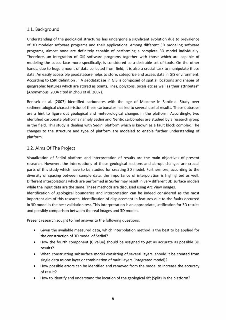
Sardinia is the second largest island in Mediterranean Sea after Sicily (Figure 1). The area is around

24090 km2 consisting of subtropical carbonates which are kinds of fault-block platforms (Benisek et

al. 2007). This area offers an amazing geology in a relatively small area (Spinosa n.d). The area under

study constitutes of carbonates with the age of Miocene (A subdivision of geological era, Tertiary,

with age of 5-24 million years). In more detail, a 19 km2 area named Sedini is a carbonate platform

which is the area where this study is concentrated on. Observation of several unconformities in

Sedini platform implies existence of fault in this structure. Consequently there are not only temporal

changes in carbonate’s attributes, but also changes in the depositional geometry. From geological

point of view, there is a NW-SE rift in the carbonates that affected the structure of the carbonates

and consequently addresses two types of the preliminary structure related to warm water and cool

water carbonates in Sardinia (Benisek et al. in press).

Figure 1. Geographical location of Sardinia in Italy (http://www.e-rcps.com)

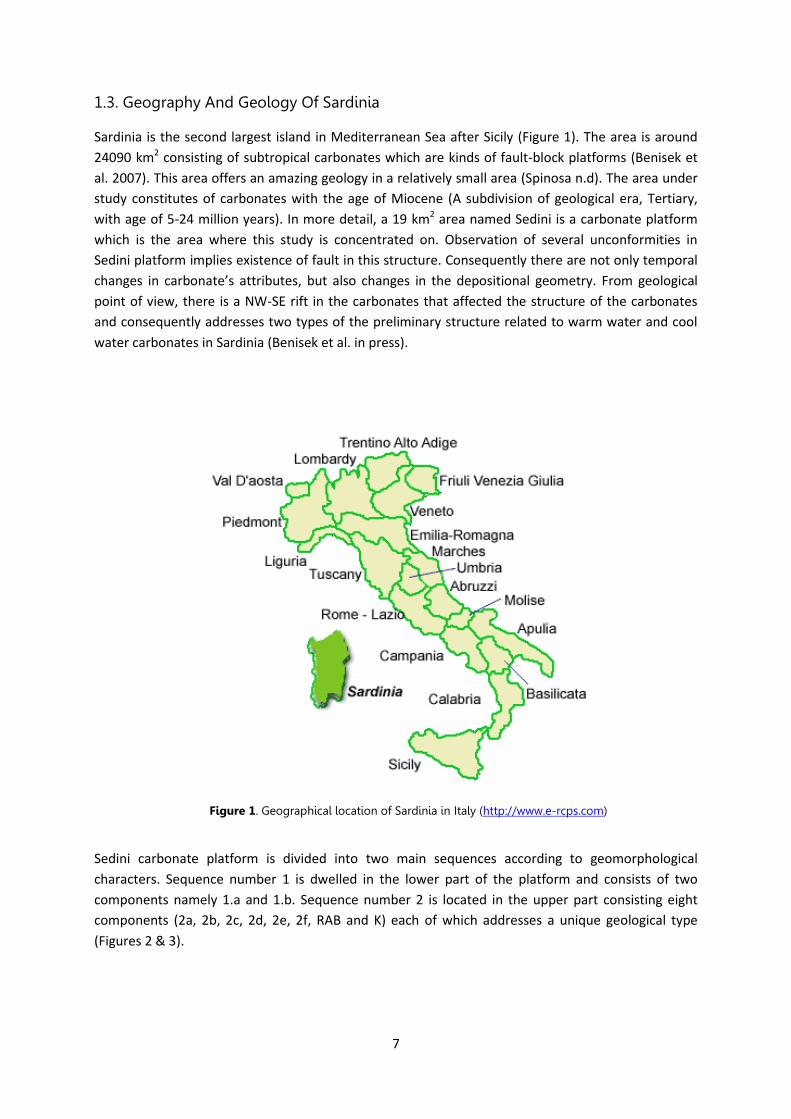
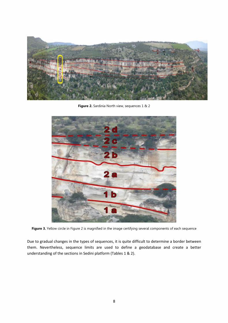
Sedini carbonate platform is divided into two main sequences according to geomorphological

characters. Sequence number 1 is dwelled in the lower part of the platform and consists of two

components namely 1.a and 1.b. Sequence number 2 is located in the upper part consisting eight

components (2a, 2b, 2c, 2d, 2e, 2f, RAB and K) each of which addresses a unique geological type

(Figures 2 & 3).

8

Figure 2. Sardinia North view, sequences 1 & 2

Figure 3. Yellow circle in Figure 2 is magnified in the image certifying several components of each sequence

Due to gradual changes in the types of sequences, it is quite difficult to determine a border between

them. Nevertheless, sequence limits are used to define a geodatabase and create a better

understanding of the sections in Sedini platform (Tables 1 & 2).

9

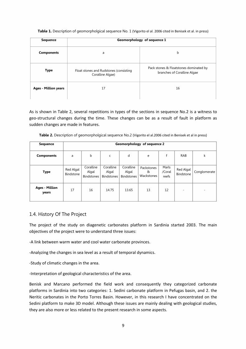
Table 1. Description of geomorpholgical sequence No. 1 (Vigorito el al. 2006 cited in Benisek et al. in press)

As is shown in Table 2, several repetitions in types of the sections in sequence No.2 is a witness to

geo-structural changes during the time. These changes can be as a result of fault in platform as

sudden changes are made in features.

Table 2. Description of geomorpholgical sequence No.2 (Vigorito el al.2006 cited in Benisek et al in press)

1.4. History Of The Project

The project of the study on diagenetic carbonates platform in Sardinia started 2003. The main

objectives of the project were to understand three issues:

-A link between warm water and cool water carbonate provinces.

-Analyzing the changes in sea level as a result of temporal dynamics.

-Study of climatic changes in the area.

-Interpretation of geological characteristics of the area.

Benisk and Marcano performed the field work and consequently they categorized carbonate

platforms in Sardinia into two categories: 1. Sedini carbonate platform in Pefugas basin, and 2. the

Neritic carbonates in the Porto Torres Basin. However, in this research I have concentrated on the

Sedini platform to make 3D model. Although these issues are mainly dealing with geological studies,

they are also more or less related to the present research in some aspects.

Sequence Geomorphology of sequence 1

Components a b

Type Float stones and Rudstones (consisting Coralline Algae)

Pack stones & Floatstones dominated by branches of Coralline Algae

Ages - Million years 17 16

Sequence Geomorphology of sequence 2

Components a b c d e f RAB k

Type Red Algal Bindstone

Coralline Algal

Bindstones

Coralline Algal

Bindstones

Coralline Algal

Bindstones

Packstones &

Wackstones

Marls /Coral reefs

Red Algal Bindstone

Conglomerate

Ages - Million years 17 16 14.75 13.65 13 12 - -

10

2. Previous Scientific Studies

Zhou et al. (2007) have done a research to create a comprehensive geodatabase for a geological

purpose consisting of two parts: The integrated geodatabase which is normally used to store data,

points, images etc and a regularized 2.5D geodatabase. The regularized geodatabase is a suitable tool

for 3D analysis extension works for solid models. So if regularized geodatabase is designed, the

implementation of 3D analysis is applicable in the geodatabase. In other words, Zhou et al. (2007)

developed this idea to consider 2.5D geodatabase to store boundaries of ore body and volume

related works as well as estimation of ore body at any location. But 3D analysis tools cannot be used

for this study since it is unable to construct the solid 3D model. Morover, Voxler is unable to export

files from Voxler format to ESRI to be used for 3D analysis works.

For the cases where geodatabase is used for geological data, Gustavsson et al. (2007) outlined a

geomorphologic transformation from conventional paper maps into a geodatabase. In their research,

it is discussed how DEM and satellite images can jointly provide possibility of interpretation of the

results. The study also emphasized the importance of storing original data as separated from those

which has undergone changes during the work process. The procedure consists of five main steps to

define five datasets according to available set of data. The result of study indicates that not all of the

transformations into GIS database are equally easy, but several feature transformations still need to

be more studied. The methodology enables facilitation of further analysis using basemap to visualize

uncertain borders.

As interpolation methodology, Lu and Wong (2007) in their research tried to develop a way to

increase the accuracy of the result when doing IDW interpolation. The idea was based on the

adaptive distance decay parameter rather than a constant parameter. Methodology assumes that

the weights which are being assigned to the points are dependent upon spatial patterns of neighbors

as well. The result of their study increased the accuracy compared to traditional IDW. Their

methodology, AIDW (Adaptive inverse distance weighted) is especially helpful in the cases where an

intensive change in a small area happens. The method was well discussed as a helpful hint for future

interpolation studies.

In addition, Tacher et al. (2006) worked on uncertainties of 3D subsurface model. They studied the

geological constraints which can be useful providing details of uncertainties. They elaborated how

the result of 3D model projects may differ from the reality and geological interfaces. Their

methodology is therefore a hint to identify uncertainties of 3D result when interpretation is being

done.

With regards to the importance of implementation of reliable data collected from field, Kaufmann

and Thierry (2007) have conducted a research in 3D modeling of subsurface geological features. They

also have focused on the significance of interpretation of the result. The result of interpretation

according to their research is dependent on the observer’s understanding as well as geological

knowledge of interpreter. In their research, they noted that in some studies it is needed to omit

certain types of errors from available data in order to get reliable results. Also, the interaction

between geodatabase and GIS tools with Gocad is discussed. There exist conditions that according to

the related study can lead to increase in the accuracy of results. Among them are: Complete and

enough number of field data, quality and desperation of these data over the area of study.

11

Moreover, the complicated and important task of interpretation of result is taken into account when

data are sparse over the area.

The similar research to present study was done as 3D reconstruction of geological bodies with

complex structure by Zanchi et al. (2007). The integration of GIS and Gocad helps to export and

import features of interest between software. The study was focused on three Italian alp units and

structural geological sections are evaluated after 3D construction. 3D visualization of models led to

accurate result to interpretation of structural geology studies. The result of study also emphasized

the importance of 3D modeling to avoid unrealistic interpretation of in depth studies. This is in fact

one of the most important advantages of 3D modeling for geological studies.

3. Material And Method

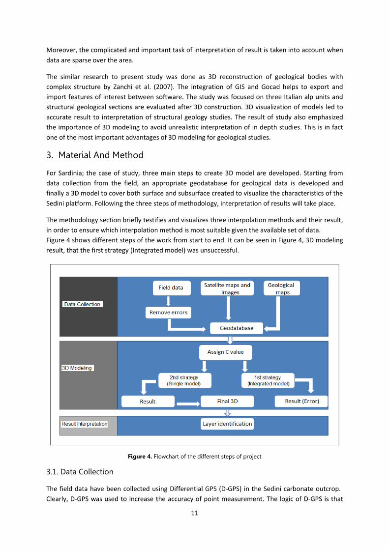
For Sardinia; the case of study, three main steps to create 3D model are developed. Starting from

data collection from the field, an appropriate geodatabase for geological data is developed and

finally a 3D model to cover both surface and subsurface created to visualize the characteristics of the

Sedini platform. Following the three steps of methodology, interpretation of results will take place.

The methodology section briefly testifies and visualizes three interpolation methods and their result,

in order to ensure which interpolation method is most suitable given the available set of data.

Figure 4 shows different steps of the work from start to end. It can be seen in Figure 4, 3D modeling

result, that the first strategy (Integrated model) was unsuccessful.

Figure 4. Flowchart of the different steps of project

3.1. Data Collection

The field data have been collected using Differential GPS (D-GPS) in the Sedini carbonate outcrop.

Clearly, D-GPS was used to increase the accuracy of point measurement. The logic of D-GPS is that

12

first ground based stations receive signals then these stations will be read based on a known point.

The differential is the difference between known locations and GPS reading which can therefore

increase accuracy of the reading results. Given the special patterns of the geological sections and

discontinuous parts, which are interrupted suddenly by faults, GPS data are stored with various

spacing intervals; nevertheless, since the geography is complex, the results will suffer more

compared with simple geography if the same data points are used. In Sedini, geological boundaries

were observed from three geographical views of the platform; North, South, West. However,

sometimes combination of these views is more appropriate to address these boundaries. The point

coordinates including x, y and z values from different views of the field were stored to create

geodatabase and perform interpolation. However, collection of data was based on the needs of

project. In other words, since the main objective of project is the study of geological characteristics

of the area, only main geological layers considered to be measured using D-GPS. Although part of

these features of interest, marked with red lines in Figure 2, are considered as appropriate set of

data to achieve the result, they do not necessarily suffice.

The boundaries listed in Table 3 are all features which contain available sample data of the field.

According to Table 3, some features are presented in more than one view of the platform. This can

later be used to check presence of the features in the model. The geological boundaries have got

their name according to Table 1 and Table 2 i.e. L represent line boundary between two layers and

next two codes each represent the number of sequences and types of components. For instance

L_1b_Rab means the boundary line which occurs between layer b in sequence 1 and layer Rab

(Which is in sequence 2).

Table 3. Geological boundaries and their corresponding existing views

Geological Boundary View of Occurrence in Sedini

L_1a_1b North/South

L_1b_2a North

L_1b_Rab North/South

L_2a_Rab North/South

L_2a_2b North/South

L_2b_2c North/South

L_2c_2d North/South

L_2d_2e North/South/ West

L_2e_2f West

L_1a_K North

However, it is important to include all of the boundary layers in the final 3D model unless they may

lead to some errors. The study of the coordinates between features and distance between them in

the images prove that there is an extremely long distance in some cases which has to be validated in

a model. Furthermore, the sample data are collected based on the needs only from several lines in

13

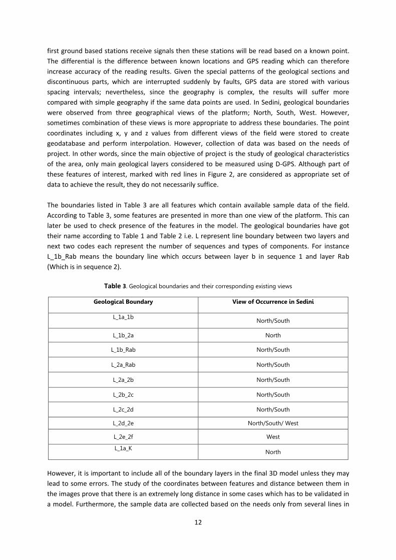
the surface. Obviously presence of data from different depth and locations would result in a more

accurate model. In cases where a gap is occurred or the data do not suffice for any reason, different

attributes of the points such as point numbers or date act as a trace to find out area of interest.

However the said attributes are occasionally mixed up or disrupted. Below, Figure 5 is a 3D scatter

plot of Sedini platform indicating how points are distributed in x, y and z directions.

Figure 5. 3D XYZ Line/Scatter plot of Sedini platform

3.2. Development Of Geodatabase

According to Dangermond (2006), preparation a geodatabase can be regarded as an unavoidable

step in geological studies. The varieties of functionalities beside its simplicity led to prevalence of

geodatabase in recent years in most of the fields of sciences including geomatics and geology. A

geodatabase, as a tool in geological study, can contain data of spatial locations and shapes of

geological or geographical structures which are saved as three main categories of point (Shape), line

and polygon (Zhou et al. 2007). In ArcGIS package, ArcCatalogue is capable to create a personal

geodatabase. Normally, features with the same types of attributes should be located in a certain

dataset. Two main datasets in this study are considered according to the available geographical data;

Sardinia North and Sardinia South. In ArcCatalogue, after defining a personal geodatabse, the two

mentioned geodatasets address the correct coordinate positions. Since the study field is located in

UTM 32 N, it is necessary to deal with two datasets in the corresponding coordinate system. The

14

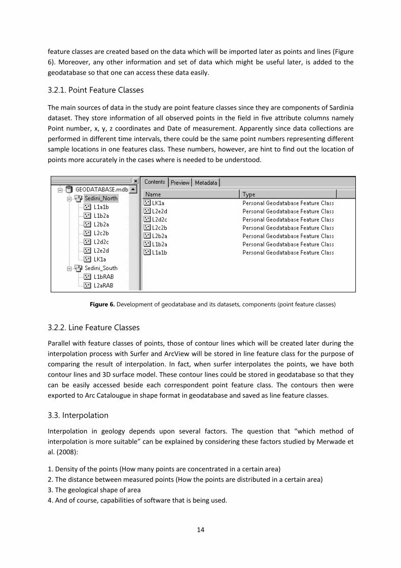
feature classes are created based on the data which will be imported later as points and lines (Figure

6). Moreover, any other information and set of data which might be useful later, is added to the

geodatabase so that one can access these data easily.

3.2.1. Point Feature Classes

The main sources of data in the study are point feature classes since they are components of Sardinia

dataset. They store information of all observed points in the field in five attribute columns namely

Point number, x, y, z coordinates and Date of measurement. Apparently since data collections are

performed in different time intervals, there could be the same point numbers representing different

sample locations in one features class. These numbers, however, are hint to find out the location of

points more accurately in the cases where is needed to be understood.

Figure 6. Development of geodatabase and its datasets, components (point feature classes)

3.2.2. Line Feature Classes

Parallel with feature classes of points, those of contour lines which will be created later during the

interpolation process with Surfer and ArcView will be stored in line feature class for the purpose of

comparing the result of interpolation. In fact, when surfer interpolates the points, we have both

contour lines and 3D surface model. These contour lines could be stored in geodatabase so that they

can be easily accessed beside each correspondent point feature class. The contours then were

exported to Arc Catalougue in shape format in geodatabase and saved as line feature classes.

3.3. Interpolation

Interpolation in geology depends upon several factors. The question that “which method of

interpolation is more suitable” can be explained by considering these factors studied by Merwade et

al. (2008):

1. Density of the points (How many points are concentrated in a certain area)

2. The distance between measured points (How the points are distributed in a certain area)

3. The geological shape of area

4. And of course, capabilities of software that is being used.

15

These factors however, are only part of criterias which Merwade et al. (2008) have taken into

account in their study. Given the above mentioned conditions in terms of importance of

interpolation, it is quite important to first review these conditions and then proceed to initiate the

intepolation process. Accordingly, three main interpolation methods are evaluated to compare the

result and differences between them. Kriging, IDW and Spline are examined since they are the most

common interpolation methods used in geological studies.

3.3.1. Interpolation Of Sardinia Sample Data

As noted in the data collection section, the field data were measured in Sardinia according to the

needs of the project. The spacing of the measured points is not equal. The platform in Sedini

measured an area of around 19 km2 .

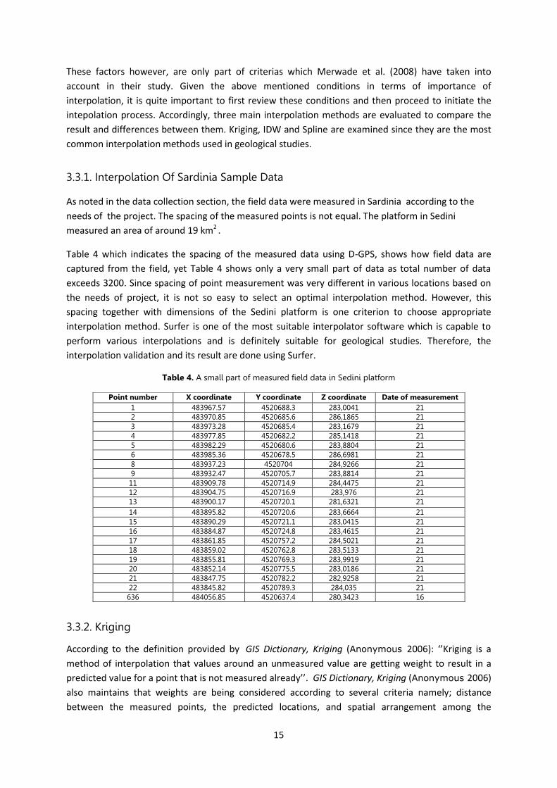
Table 4 which indicates the spacing of the measured data using D-GPS, shows how field data are

captured from the field, yet Table 4 shows only a very small part of data as total number of data

exceeds 3200. Since spacing of point measurement was very different in various locations based on

the needs of project, it is not so easy to select an optimal interpolation method. However, this

spacing together with dimensions of the Sedini platform is one criterion to choose appropriate

interpolation method. Surfer is one of the most suitable interpolator software which is capable to

perform various interpolations and is definitely suitable for geological studies. Therefore, the

interpolation validation and its result are done using Surfer.

Table 4. A small part of measured field data in Sedini platform

3.3.2. Kriging

According to the definition provided by GIS Dictionary, Kriging (Anonymous 2006): ‘’Kriging is a

method of interpolation that values around an unmeasured value are getting weight to result in a

predicted value for a point that is not measured already’’. GIS Dictionary, Kriging (Anonymous 2006)

also maintains that weights are being considered according to several criteria namely; distance

between the measured points, the predicted locations, and spatial arrangement among the

Point number X coordinate Y coordinate Z coordinate Date of measurement 1 483967.57 4520688.3 283,0041 21 2 483970.85 4520685.6 286,1865 21 3 483973.28 4520685.4 283,1679 21 4 483977.85 4520682.2 285,1418 21 5 483982.29 4520680.6 283,8804 21 6 483985.36 4520678.5 286,6981 21 8 483937.23 4520704 284,9266 21 9 483932.47 4520705.7 283,8814 21 11 483909.78 4520714.9 284,4475 21 12 483904.75 4520716.9 283,976 21 13 483900.17 4520720.1 281,6321 21 14 483895.82 4520720.6 283,6664 21 15 483890.29 4520721.1 283,0415 21 16 483884.87 4520724.8 283,4615 21 17 483861.85 4520757.2 284,5021 21 18 483859.02 4520762.8 283,5133 21 19 483855.81 4520769.3 283,9919 21 20 483852.14 4520775.5 283,0186 21 21 483847.75 4520782.2 282,9258 21 22 483845.82 4520789.3 284,035 21 636 484056.85 4520637.4 280,3423 16

16

measured points. In Kriging it acts also as if there are homogenous patterns and characteristics all

over the area (GIS dictionary, Kriging, Anonymous 2006). In the Sedini platform however, there are

relatively harsh discrepancies that make it difficult to use Kriging for interpolation. Nevertheless, this

issue could be resolvable if interpolation is done for the area divided to several homogenous parts.

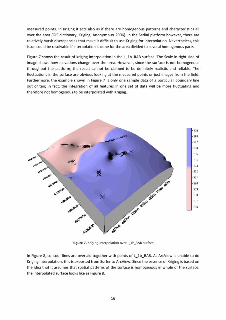
Figure 7 shows the result of kriging interpolation in the L_1b_RAB surface. The Scale in right side of

image shows how elevations change over the area. However, since the surface is not homogenous

throughout the platform, the result cannot be claimed to be definitely realistic and reliable. The

fluctuations in the surface are obvious looking at the measured points or just images from the field.

Furthermore, the example shown in Figure 7 is only one sample data of a particular boundary line

out of ten; in fact, the integration of all features in one set of data will be more fluctuating and

therefore not homogenous to be interpolated with Kriging.

Figure 7. Kriging interpolation over L_1b_RAB surface

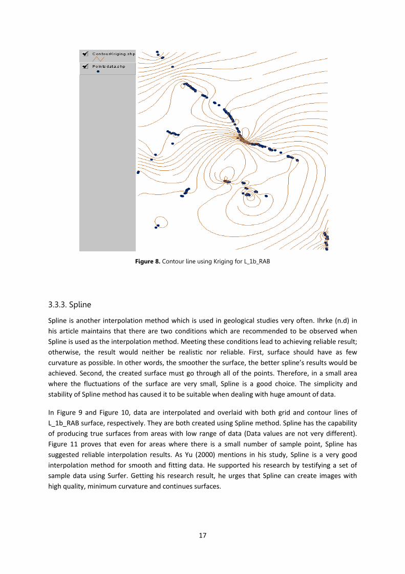
In Figure 8, contour lines are overlaid together with points of L_1b_RAB. As ArcView is unable to do

Kriging interpolation; this is exported from Surfer to ArcView. Since the essence of Kriging is based on

the idea that it assumes that spatial patterns of the surface is homogenous in whole of the surface,

the interpolated surface looks like as Figure 8.

17

Figure 8. Contour line using Kriging for L_1b_RAB

3.3.3. Spline

Spline is another interpolation method which is used in geological studies very often. Ihrke (n.d) in

his article maintains that there are two conditions which are recommended to be observed when

Spline is used as the interpolation method. Meeting these conditions lead to achieving reliable result;

otherwise, the result would neither be realistic nor reliable. First, surface should have as few

curvature as possible. In other words, the smoother the surface, the better spline’s results would be

achieved. Second, the created surface must go through all of the points. Therefore, in a small area

where the fluctuations of the surface are very small, Spline is a good choice. The simplicity and

stability of Spline method has caused it to be suitable when dealing with huge amount of data.

In Figure 9 and Figure 10, data are interpolated and overlaid with both grid and contour lines of

L_1b_RAB surface, respectively. They are both created using Spline method. Spline has the capability

of producing true surfaces from areas with low range of data (Data values are not very different).

Figure 11 proves that even for areas where there is a small number of sample point, Spline has

suggested reliable interpolation results. As Yu (2000) mentions in his study, Spline is a very good

interpolation method for smooth and fitting data. He supported his research by testifying a set of

sample data using Surfer. Getting his research result, he urges that Spline can create images with

high quality, minimum curvature and continues surfaces.

18

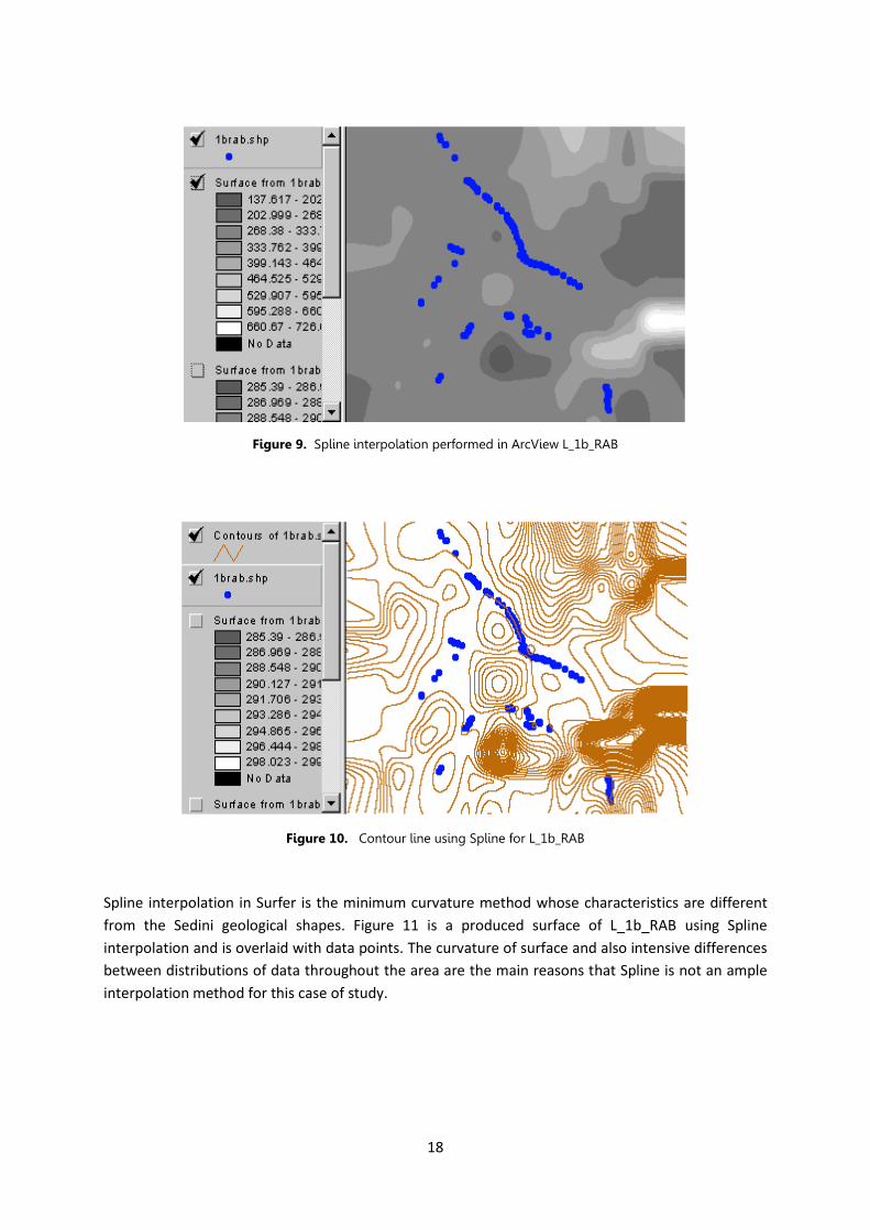
Figure 9. Spline interpolation performed in ArcView L_1b_RAB

Figure 10. Contour line using Spline for L_1b_RAB

Spline interpolation in Surfer is the minimum curvature method whose characteristics are different

from the Sedini geological shapes. Figure 11 is a produced surface of L_1b_RAB using Spline

interpolation and is overlaid with data points. The curvature of surface and also intensive differences

between distributions of data throughout the area are the main reasons that Spline is not an ample

interpolation method for this case of study.

19

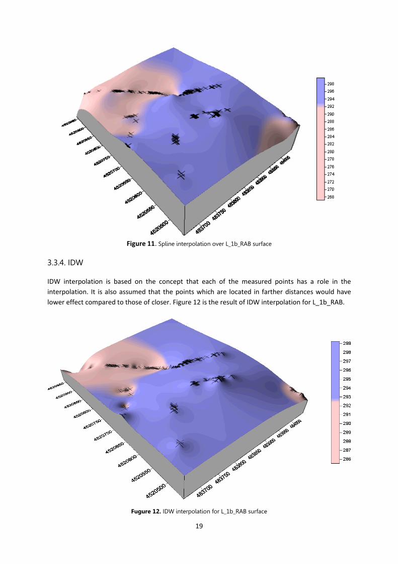
Figure 11. Spline interpolation over L_1b_RAB surface

3.3.4. IDW IDW interpolation is based on the concept that each of the measured points has a role in the

interpolation. It is also assumed that the points which are located in farther distances would have

lower effect compared to those of closer. Figure 12 is the result of IDW interpolation for L_1b_RAB.

Fugure 12. IDW interpolation for L_1b_RAB surface

20

Indeed, IDW interpolation can be accomplished when the data points are spaced dense enough, so

that the fluctuation in the surface can interfere in the surface’s shape (Childes 2004). Since the

method is based on the distance of points from the location of predicted output cell (the assigned

weight), the distance between points are definitely important. However, according to Lu and Wong

(2007), the method besides possessing advantages such as appropriate speed in operation and

simplicity, has its own shortages. They maintain that not only the same weight should be assigned for

all of the study area irrespective to distribution of data, but a weight according to patterns of the

neighbors around un-sampled points should be kept in mind. In other words, this weight should be

based on characteristics of neighbors around un-sampled points instead of only distance to the

closest sample points (Lu and Wong 2007).

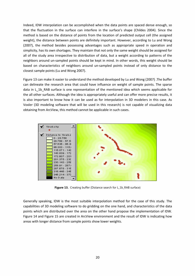
Figure 13 can make it easier to understand the method developed by Lu and Wong (2007) .The buffer

can delineate the research area that could have influence on weight of sample points. The sparse

data in L_1b_RAB surface is one representation of the mentioned idea which seems applicable for

the all other surfaces. Although the idea is appropriately useful and can offer more precise results, it

is also important to know how it can be used as for interpolation in 3D modelers in this case. As

Voxler (3D modeling software that will be used in this research) is not capable of visualizing data

obtaining from ArcView, this method cannot be applicable in such cases.

Figure 13. Creating buffer (Distance search for L_1b_RAB surface)

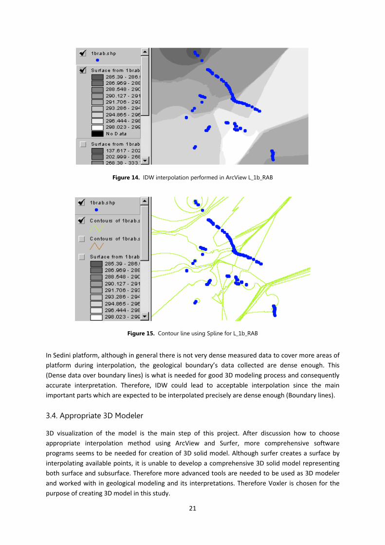
Generally speaking, IDW is the most suitable interpolation method for the case of this study. The

capabilities of 3D modeling software to do gridding on the one hand, and characteristics of the data

points which are distributed over the area on the other hand propose the implementation of IDW.

Figure 14 and Figure 15 are created in ArcView environment and the result of IDW is indicating how

areas with longer distance from sample points show lower weights.

21

Figure 14. IDW interpolation performed in ArcView L_1b_RAB

Figure 15. Contour line using Spline for L_1b_RAB

In Sedini platform, although in general there is not very dense measured data to cover more areas of

platform during interpolation, the geological boundary’s data collected are dense enough. This

(Dense data over boundary lines) is what is needed for good 3D modeling process and consequently

accurate interpretation. Therefore, IDW could lead to acceptable interpolation since the main

important parts which are expected to be interpolated precisely are dense enough (Boundary lines).

3.4. Appropriate 3D Modeler

3D visualization of the model is the main step of this project. After discussion how to choose

appropriate interpolation method using ArcView and Surfer, more comprehensive software

programs seems to be needed for creation of 3D solid model. Although surfer creates a surface by

interpolating available points, it is unable to develop a comprehensive 3D solid model representing

both surface and subsurface. Therefore more advanced tools are needed to be used as 3D modeler

and worked with in geological modeling and its interpretations. Therefore Voxler is chosen for the

purpose of creating 3D model in this study.

22

3.4.1. Voxler Interpolation

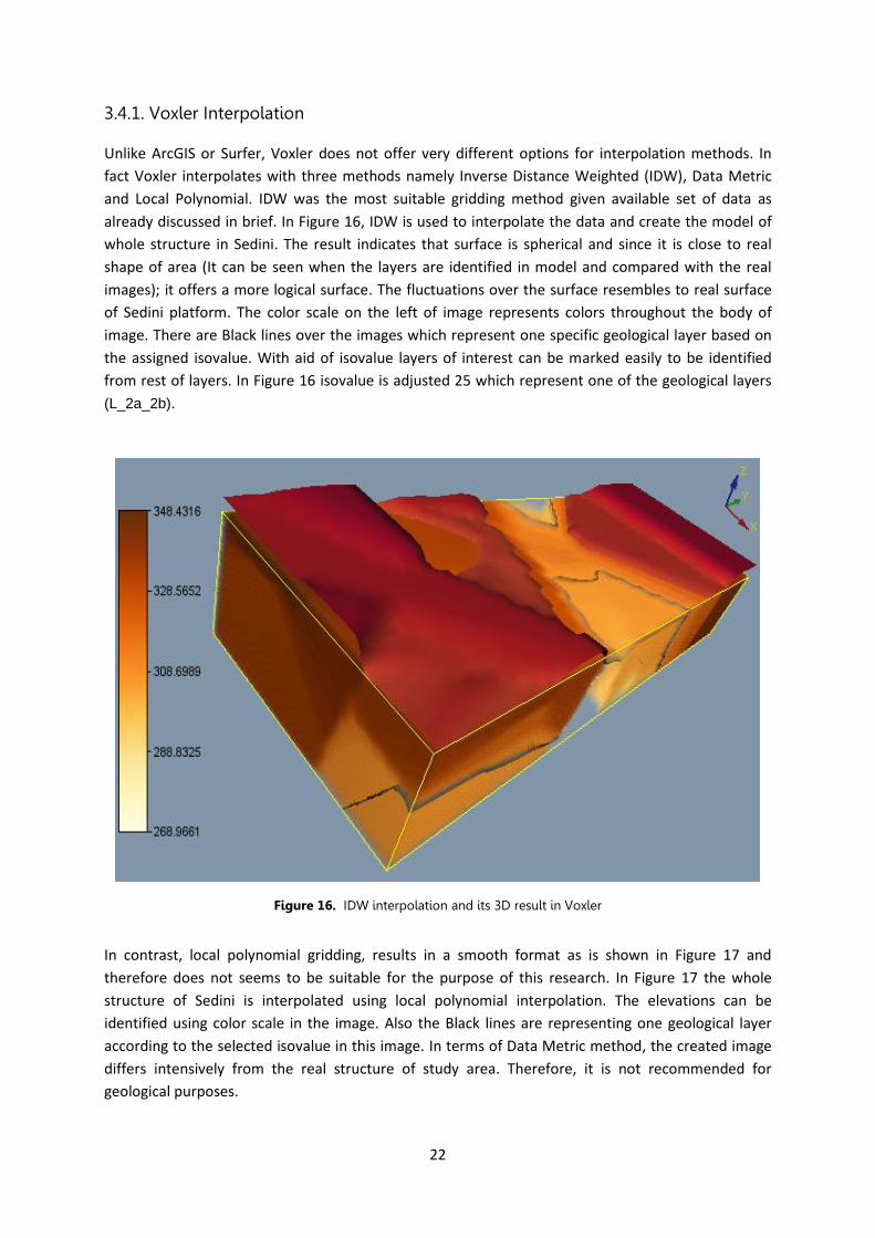
Unlike ArcGIS or Surfer, Voxler does not offer very different options for interpolation methods. In

fact Voxler interpolates with three methods namely Inverse Distance Weighted (IDW), Data Metric

and Local Polynomial. IDW was the most suitable gridding method given available set of data as

already discussed in brief. In Figure 16, IDW is used to interpolate the data and create the model of

whole structure in Sedini. The result indicates that surface is spherical and since it is close to real

shape of area (It can be seen when the layers are identified in model and compared with the real

images); it offers a more logical surface. The fluctuations over the surface resembles to real surface

of Sedini platform. The color scale on the left of image represents colors throughout the body of

image. There are Black lines over the images which represent one specific geological layer based on

the assigned isovalue. With aid of isovalue layers of interest can be marked easily to be identified

from rest of layers. In Figure 16 isovalue is adjusted 25 which represent one of the geological layers

(L_2a_2b).

Figure 16. IDW interpolation and its 3D result in Voxler

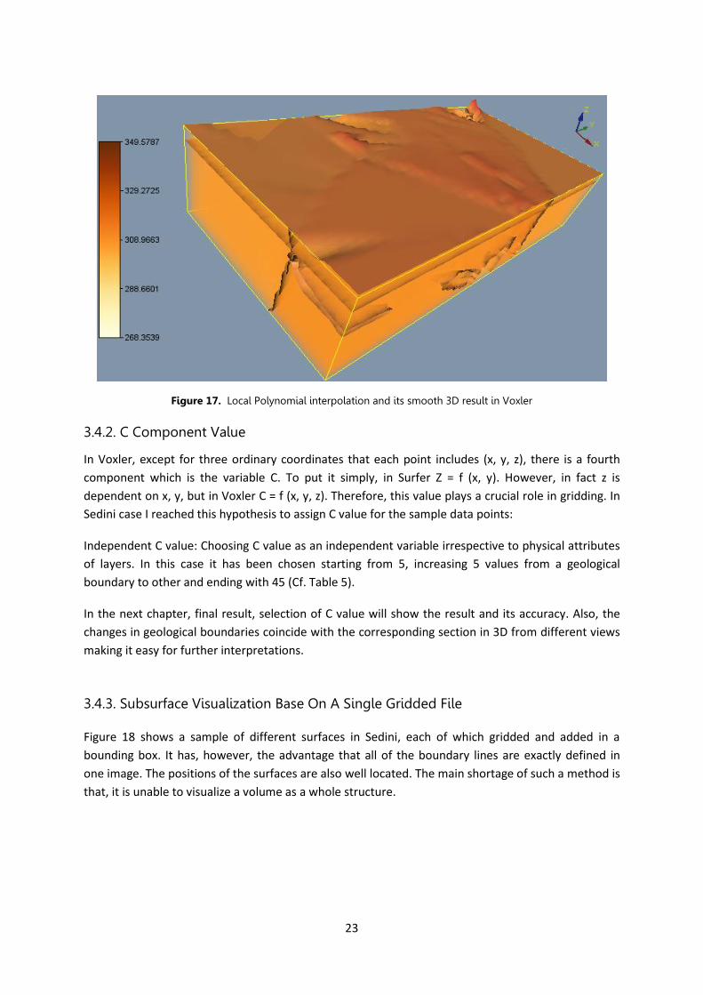
In contrast, local polynomial gridding, results in a smooth format as is shown in Figure 17 and

therefore does not seems to be suitable for the purpose of this research. In Figure 17 the whole

structure of Sedini is interpolated using local polynomial interpolation. The elevations can be

identified using color scale in the image. Also the Black lines are representing one geological layer

according to the selected isovalue in this image. In terms of Data Metric method, the created image

differs intensively from the real structure of study area. Therefore, it is not recommended for

geological purposes.

23

Figure 17. Local Polynomial interpolation and its smooth 3D result in Voxler

3.4.2. C Component Value

In Voxler, except for three ordinary coordinates that each point includes (x, y, z), there is a fourth

component which is the variable C. To put it simply, in Surfer Z = f (x, y). However, in fact z is

dependent on x, y, but in Voxler C = f (x, y, z). Therefore, this value plays a crucial role in gridding. In

Sedini case I reached this hypothesis to assign C value for the sample data points:

Independent C value: Choosing C value as an independent variable irrespective to physical attributes

of layers. In this case it has been chosen starting from 5, increasing 5 values from a geological

boundary to other and ending with 45 (Cf. Table 5).

In the next chapter, final result, selection of C value will show the result and its accuracy. Also, the

changes in geological boundaries coincide with the corresponding section in 3D from different views

making it easy for further interpretations.

3.4.3. Subsurface Visualization Base On A Single Gridded File Figure 18 shows a sample of different surfaces in Sedini, each of which gridded and added in a

bounding box. It has, however, the advantage that all of the boundary lines are exactly defined in

one image. The positions of the surfaces are also well located. The main shortage of such a method is

that, it is unable to visualize a volume as a whole structure.

24

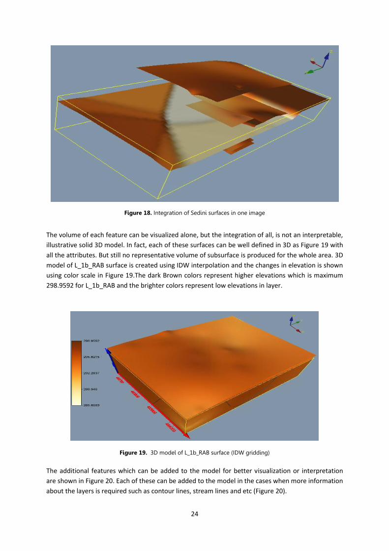
Figure 18. Integration of Sedini surfaces in one image The volume of each feature can be visualized alone, but the integration of all, is not an interpretable,

illustrative solid 3D model. In fact, each of these surfaces can be well defined in 3D as Figure 19 with

all the attributes. But still no representative volume of subsurface is produced for the whole area. 3D

model of L_1b_RAB surface is created using IDW interpolation and the changes in elevation is shown

using color scale in Figure 19.The dark Brown colors represent higher elevations which is maximum

298.9592 for L_1b_RAB and the brighter colors represent low elevations in layer.

Figure 19. 3D model of L_1b_RAB surface (IDW gridding)

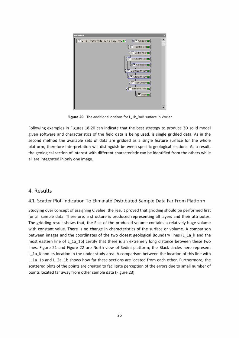
The additional features which can be added to the model for better visualization or interpretation

are shown in Figure 20. Each of these can be added to the model in the cases when more information

about the layers is required such as contour lines, stream lines and etc (Figure 20).

25

Figure 20. The additional options for L_1b_RAB surface in Voxler

Following examples in Figures 18-20 can indicate that the best strategy to produce 3D solid model

given software and characteristics of the field data is being used, is single gridded data. As in the

second method the available sets of data are gridded as a single feature surface for the whole

platform, therefore interpretation will distinguish between specific geological sections. As a result,

the geological section of interest with different characteristic can be identified from the others while

all are integrated in only one image.

4. Results

4.1. Scatter Plot-Indication To Eliminate Distributed Sample Data Far From Platform

Studying over concept of assigning C value, the result proved that gridding should be performed first

for all sample data. Therefore, a structure is produced representing all layers and their attributes.

The gridding result shows that, the East of the produced volume contains a relatively huge volume

with constant value. There is no change in characteristics of the surface or volume. A comparison

between images and the coordinates of the two closest geological Boundary lines (L_1a_k and the

most eastern line of L_1a_1b) certify that there is an extremely long distance between these two

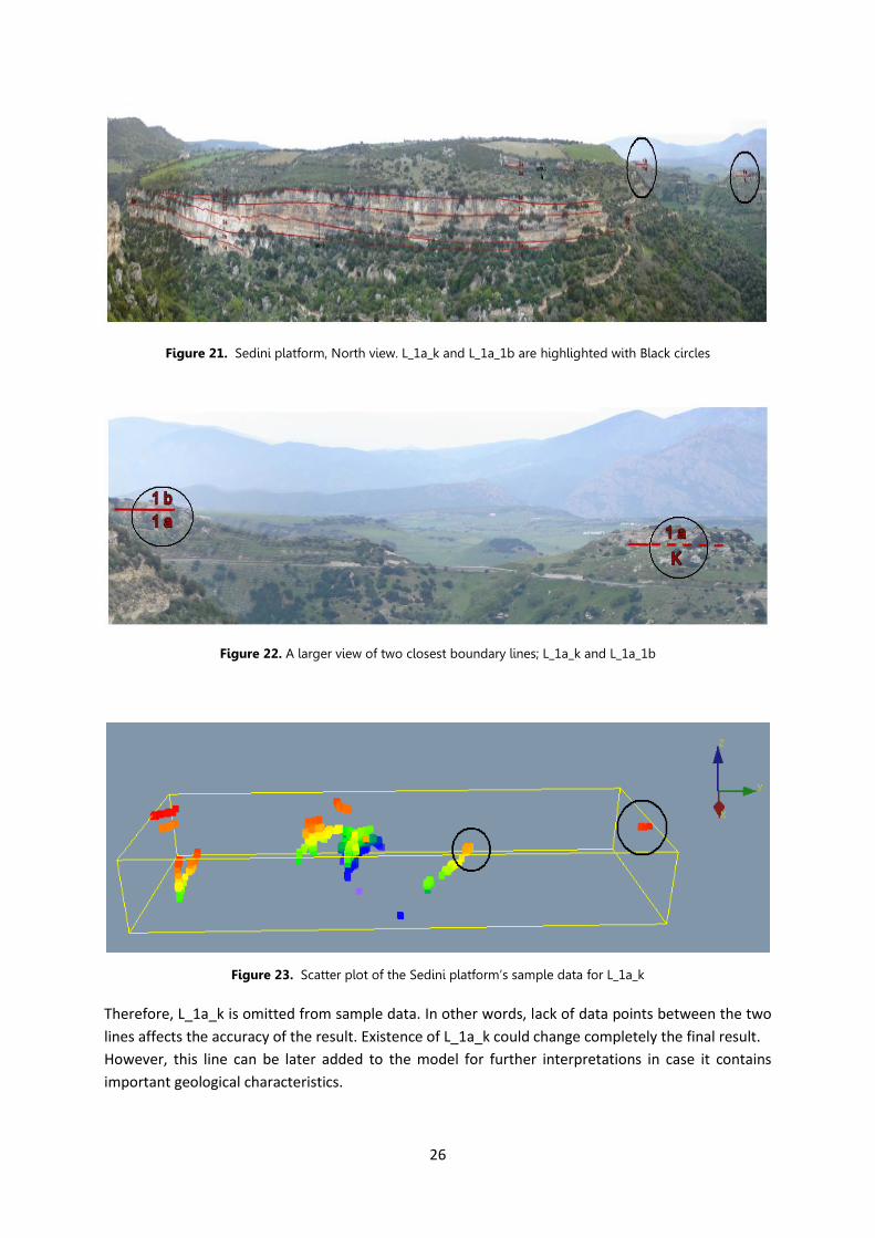
lines. Figure 21 and Figure 22 are North view of Sedini platform; the Black circles here represent

L_1a_K and its location in the under-study area. A comparison between the location of this line with

L_1a_1b and L_2a_1b shows how far these sections are located from each other. Furthermore, the

scattered plots of the points are created to facilitate perception of the errors due to small number of

points located far away from other sample data (Figure 23).

26

Figure 21. Sedini platform, North view. L_1a_k and L_1a_1b are highlighted with Black circles

Figure 22. A larger view of two closest boundary lines; L_1a_k and L_1a_1b

Figure 23. Scatter plot of the Sedini platform’s sample data for L_1a_k

Therefore, L_1a_k is omitted from sample data. In other words, lack of data points between the two

lines affects the accuracy of the result. Existence of L_1a_k could change completely the final result.

However, this line can be later added to the model for further interpretations in case it contains

important geological characteristics.

27

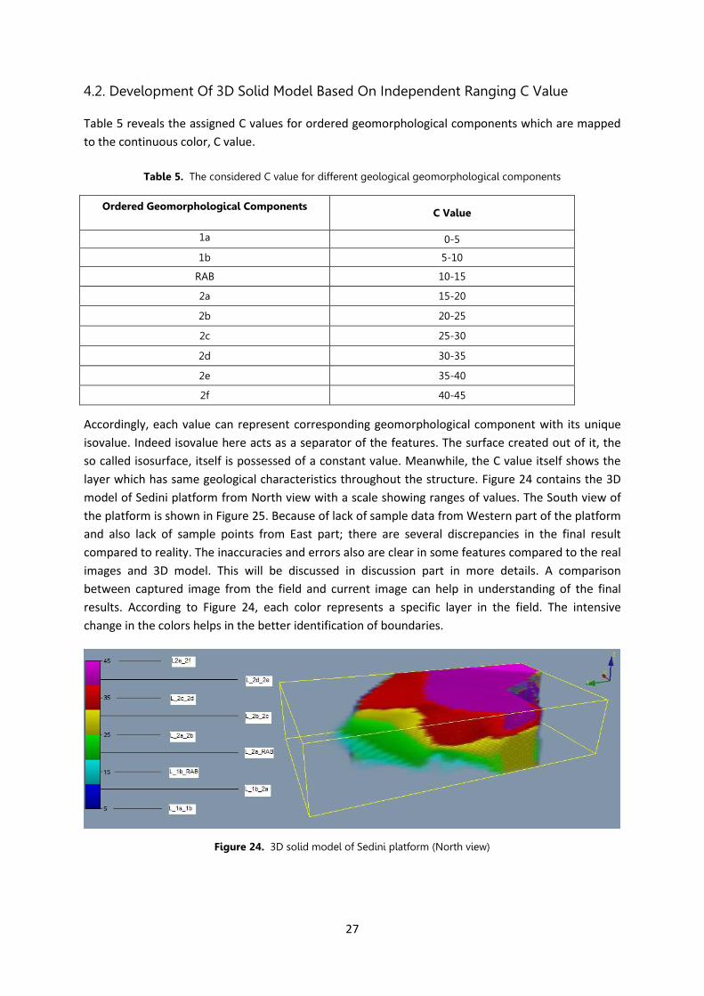
4.2. Development Of 3D Solid Model Based On Independent Ranging C Value Table 5 reveals the assigned C values for ordered geomorphological components which are mapped

to the continuous color, C value.

Table 5. The considered C value for different geological geomorphological components

Ordered Geomorphological Components C Value

1a 0-5

1b 5-10

RAB 10-15

2a 15-20

2b 20-25

2c 25-30

2d 30-35

2e 35-40

2f 40-45

Accordingly, each value can represent corresponding geomorphological component with its unique

isovalue. Indeed isovalue here acts as a separator of the features. The surface created out of it, the

so called isosurface, itself is possessed of a constant value. Meanwhile, the C value itself shows the

layer which has same geological characteristics throughout the structure. Figure 24 contains the 3D

model of Sedini platform from North view with a scale showing ranges of values. The South view of

the platform is shown in Figure 25. Because of lack of sample data from Western part of the platform

and also lack of sample points from East part; there are several discrepancies in the final result

compared to reality. The inaccuracies and errors also are clear in some features compared to the real

images and 3D model. This will be discussed in discussion part in more details. A comparison

between captured image from the field and current image can help in understanding of the final

results. According to Figure 24, each color represents a specific layer in the field. The intensive

change in the colors helps in the better identification of boundaries.

Figure 24. 3D solid model of Sedini platform (North view)

28

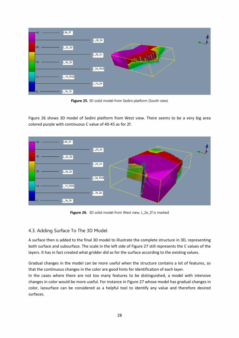
Figure 25. 3D solid model from Sedini platform (South view)

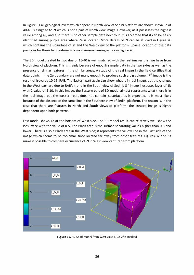
Figure 26 shows 3D model of Sedini platform from West view. There seems to be a very big area

colored purple with continuous C value of 40-45 as for 2f.

Figure 26. 3D solid model from West view, L_2e_2f is marked

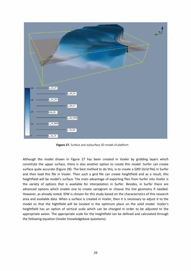
4.3. Adding Surface To The 3D Model

A surface then is added to the final 3D model to illustrate the complete structure in 3D, representing

both surface and subsurface. The scale in the left side of Figure 27 still represents the C values of the

layers. It has in fact created what gridder did as for the surface according to the existing values.

Gradual changes in the model can be more useful when the structure contains a lot of features, so

that the continuous changes in the color are good hints for identification of each layer.

In the cases where there are not too many features to be distinguished, a model with intensive

changes in color would be more useful. For instance in Figure 27 whose model has gradual changes in

color, isosurface can be considered as a helpful tool to identify any value and therefore desired

surfaces.

29

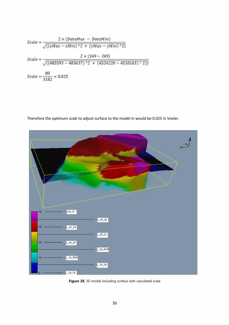
Figure 27. Surface and subsurface 3D model of platform Although the model shown in Figure 27 has been created in Voxler by gridding layers which

constitute the upper surface, there is also another option to create this model. Surfer can create

surface quite accurate (Figure 28). The best method to do this, is to create a GRD (Grid file) in Surfer

and then load this file in Voxler. Then such a gird file can create heightfield and as a result, this

heightfield will be model’s surface. The main advantage of exporting files from Surfer into Voxler is

the variety of options that is available for interpolation in Surfer. Besides, in Surfer there are

advanced options which enable one to create variogram or choose the line geometry if needed.

However, as already noted, IDW is chosen for this study based on the characteristics of this research

area and available data. When a surface is created in Voxler, then it is necessary to adjust it to the

model so that the hightfield will be located in the optimum place on the solid model. Voxler’s

heightfield has an option of vertical scale which can be changed in order to be adjusted to the

appropriate axises. The appropriate scale for the heightfield can be defined and calculated through

the following equation (Voxler knowledgebase questions):

30

Therefore the optimum scale to adjust surface to the model in would be 0.025 in Voxler.

Figure 28. 3D model including surface with calculated scale

31

5. Discussion According to the result, the main questions in this research can be answered and discussed with a short description of method of approach:

In terms of interpolation method, given characteristic of the study area, IDW interpolation method

has been chosen to construct the 3D model. When an interpolation is to be chosen, there are several

conditions which are very important to be considered such as density of data points, capability of

software, smoothness and curvature of area and etc. The idea of Lu and Wong (2007) can increase

the accuracy in final result of IDW, which has been selected. Their methodology (AIDW) is especially

good when 3D model is created using ArcGIS and similar software which are more capable to use

Adaptive Inverse Distance Weighted method within them. This is therefore a deficiency of Voxler

which is not flexible enough to be adapted to newer methodologies. Kriging could be chosen for

interpolation of surface if Voxler was able to create 3D model of each part and then add all of them

as a final model. However, Voxler is unable to interpolate surface with the Kriging method. Spline

was not chosen for interpolation since characteristic of study area does not match with the

requirements of Spline interpolation. The surface is not flat and has large variation in curvature in

many areas of Sedini platform.

C component in this thesis is chosen as an independent value irrespective to attribute of the layers. A

need to define the fourth component (C value), makes it necessary to assign appropriate values for

this component (C value). However, this value can be selected based on the attributes of the

collected data. In this research the best value for this component was examined. The independent C

value was used for gridding in Voxler since it can represent accurately coordinate of data.

Regarding The best strategy of how to create one 3D model consisting of several different layers, it is

proved that if all coordinates are collected as one file, then Voxler is able to grid it and produce the

model. However, Voxler is not capable to create a 3D model for each geological layer and then add

all of them in one 3D model. Such a combined model in Voxler (Integration of separate volumes)

could extremely differ from the real structure. Nevertheless, different software modelers have

different capabilities; one should choose the most suitable according to the needs and availabilities

of the project. Voxler is also unable to export its result to many of the leading 3D softwares. It could

be good if the final result in Voxler could be exported as ESRI files, CAD files and etc so that using

different softwares with different capabilities could improve accuracy of the final result and quality

of work.

In terms of how to deal with those of data points which could were source of errors in this study,

several issues are taken into account. The errors identified when an unusual flat area between two

set of data in the Eastern part of platform produced. With the aid of different images from field, it

revealed that this error is due to absence of data points within that large part of platform. Moreover,

the scatter plots approved the idea of producing huge flat area in the model as it can show more

accurate the distance between group of points rather than images of the field. Accordingly, since

those data points are located outside of platform, it is decided to remove those parts in order to get

more accurate result for the important areas of the model. Since some errors always will occur in

studies, one should try to eliminate them as much as possible to produce the reliable results. In this

research the main source of errors is the collected data from field. Those data do not cover the layers

32

of interest (Geological layers) as needed. Again the fourth component can be source of errors if it is

not chosen appropriately. This value is at the same time one of the best hints to eliminate errors by

helping to identify each geological layer.

Interpretation of the result is a very crucial step as two researchers can interpret a single case

differently. Based on the study of Kaufmann and Thierry (2007), interpretation of the result and the

importance of it, is considered in this study as well. They noticed some points which can affect

interpretation of the result. It has been tried to take account of those points in this study Such as

removing the source of errors as long as the final goal of project is not changed during this process.

However, several important hints are discussed in present research which are worthy to be

considered in similar studies. In this study and similar works, there are always some points which are

more accurate for checking the validity of result. The rift in the platform due to geological

phenomena in long term, differences in the C value in different layers and getting help from the

maps, images and data as much as possible will lead to more accurate results.

In terms of interpretation, not only the limited number of colors in the color scale can make it

difficult to identify features of interest in the model, but also it is impossible to have the geological

layers of interest in the exact borders between colors. This occurrence of boundary lines within one

color can be a source of error.

In case of geological studies for subsurface, the Italian Alp, case of study by Zanchi et al. (2007) was a

good hint to highlight importance of 3D modeling. It was discussed that how accurate 3D model can

improve understanding of subsurface and therefore helps to avoid inaccurate interpretations. In the

both studies of Zanchi et al. (2007) and Kaufmann and Thierry (2007) they employed both GoCad and

GIS tools together which indicates these two softwares can work good for 3D construction of

geological features. This is therefore a good idea to develop further research within these two

softwares if are accessible.

5.1. Model Interpretation With The Aid Of Isosurface

The methodology was adopted and used according to the available set of data. Compared to

previous similar studies this work offers a relatively acceptable methodology to create a 3D model.

Its simplicity also is a merit. Interpretation of the result with the aid of isosurface enables one to

examine the accuracy of the result in a more objective way. This is quite helpful to ensure

achievement of reliable results produced.

Data collection is performed based on the needs of the project. It makes it difficult in some areas to

have an accurate result. It could be more helpful to interpret the result if the sample data were

collected in an adaptive way. The geological phenomena then could be identified for instance from

East to West or inversely. This shortage was obviously a source of errors in the results since it affects

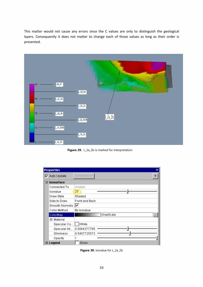
the interpretation of sections. As for a variable component (C value), C value is chosen as an

independent value. This value changes continuously as for different geomorphological components.

As it is shown in Figure 29 the isovalue can directly refer to the layer which is of interest. The yellow

circle in Figure 29 shows the opted value for L_2a_2b. However, the geological boundaries are

nominal or ranked order while the assigned C values are continuous over the whole geological body.

33

This matter would not cause any errors since the C values are only to distinguish the geological

layers. Consequently it does not matter to change each of those values as long as their order is

presented.

Figure 29. L_2a_2b is marked for interpretation

Figure 30. Isovalue for L_2a_2b

34

However, in this case, there are too many sections to visualize; it would not be possible to identify

each accurately. In fact the color scale contains a maximum of six different levels while here nine

geomorphological layers were defined to visualize. The scales with gradual changes also seem not to

be suitable since no boundary of layers is easily identifiable. Therefore, the more precise definition

for C value scale, the better the results would be.

Also, the matter of locating ground surface over the 3D model is a substantial task. If the heightfield’s

scale is not calculated according to the other data, it will show a result different from the real

structure and this can, in itself, be a source of errors.

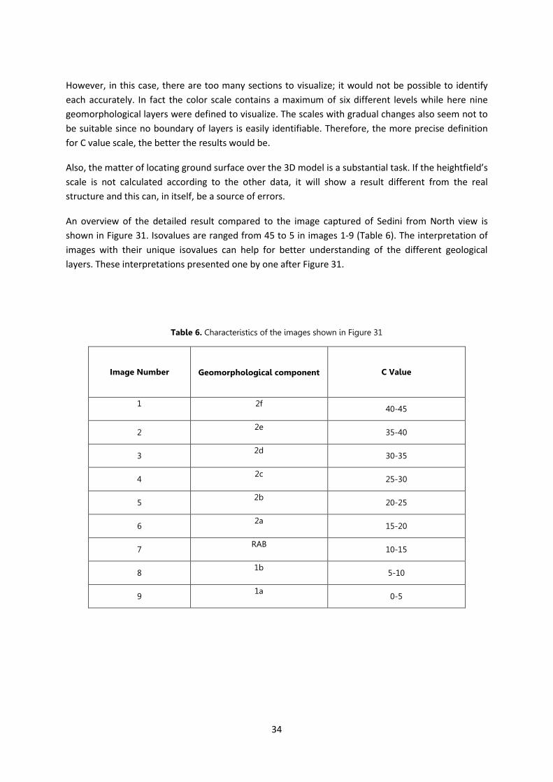
An overview of the detailed result compared to the image captured of Sedini from North view is

shown in Figure 31. Isovalues are ranged from 45 to 5 in images 1-9 (Table 6). The interpretation of

images with their unique isovalues can help for better understanding of the different geological

layers. These interpretations presented one by one after Figure 31.

Table 6. Characteristics of the images shown in Figure 31

Image Number

Geomorphological component C Value

1 2f 40-45

2 2e

35-40

3 2d

30-35

4 2c

25-30

5 2b

20-25

6 2a

15-20

7 RAB

10-15

8 1b

5-10

9 1a

0-5

35

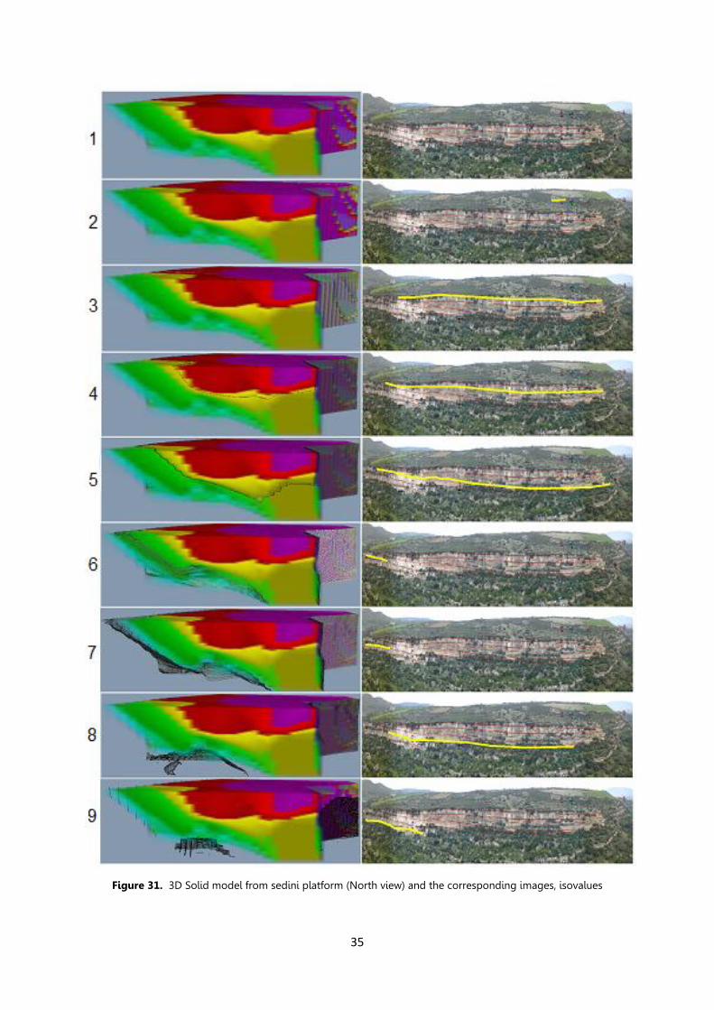
Figure 31. 3D Solid model from sedini platform (North view) and the corresponding images, isovalues

36

In Figure 31 all geological layers which appear in North view of Sedini platform are shown. Isovalue of

40-45 is assigned to 2f which is not a part of North view image. However, as it possesses the highest

value among all, and also there is no other sample data next to it, it is accepted that it can be easily

identified among purple area where 2e is located. More details of 2f can be studied in Figure 26

which contains the isosurface of 2f and the West view of the platform. Sparse location of the data

points as for these two features is a main reason causing errors in Figure 26.

The 3D model created by isovalue of 15-40 is well matched with the real images that we have from

North view of platform. This is mainly because of enough sample data in the two sides as well as the

presence of similar features in the similar areas. A study of the real image in the field certifies that

data points in the 2e boundary are not many enough to produce such a big volume. 7th image is the

result of isovalue 10-15, RAB. The Eastern part again can show what is in real image, but the changes

in the West part are due to RAB’s trend in the South view of Sedini. 8th image illustrates layer of 1b

with C value of 5-10. In this image, the Eastern part of 3D model almost represents what there is in

the real image but the western part does not contain isosurface as is expected. It is most likely

because of the absence of the same line in the Southern view of Sedini platform. The reason is, in the

case that there are features in North and South views of platform, the created image is highly

dependent upon both patterns.

Last model shows 1a at the bottom of West side. The 3D model result can relatively well show the

isosurface with the value of 0-5. The Black area is the surface separating values higher than 0-5 and

lower. There is also a Black area in the West side; it represents the yellow line in the East side of the

image which seems to be too small since located far away from other features. Figures 32 and 33

make it possible to compare occurrence of 2f in West view captured from platform.

Figure 32. 3D Solid model from West view, L_2e_2f is marked

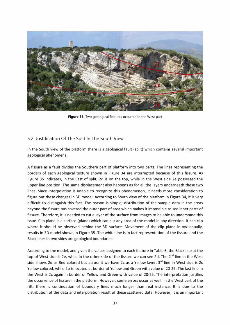
37

Figure 33. Two geological features occurred in the West part

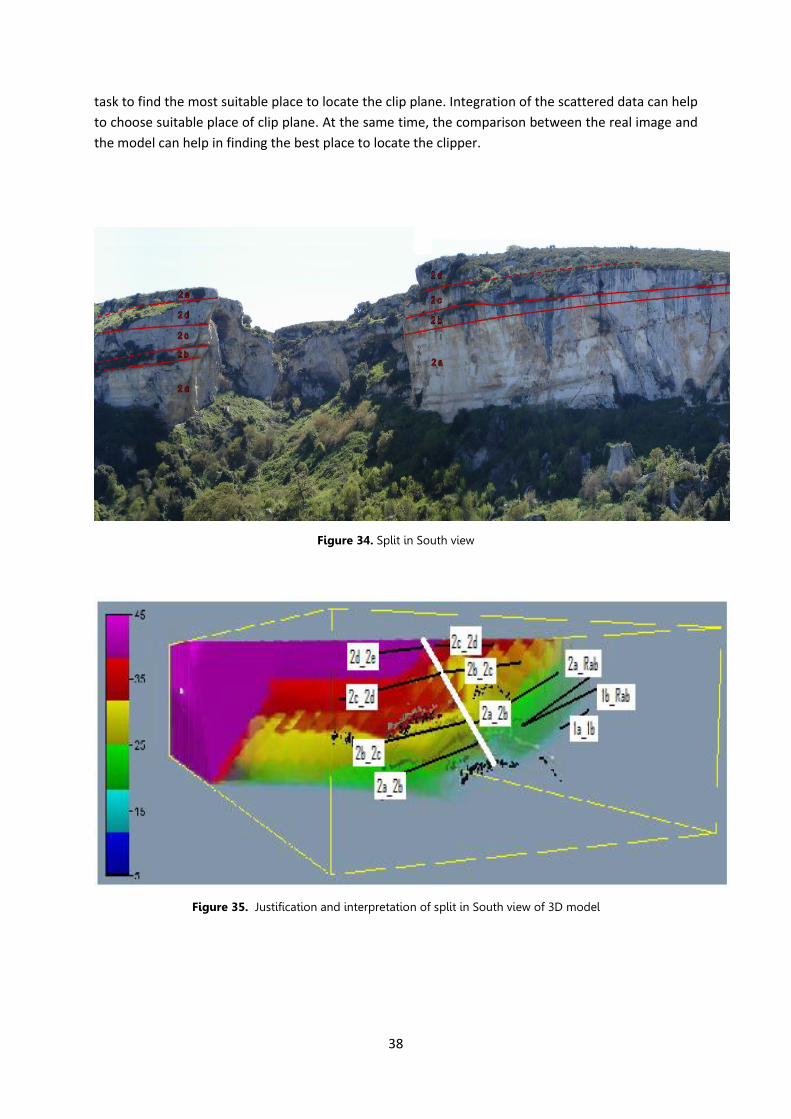
5.2. Justification Of The Split In The South View In the South view of the platform there is a geological fault (split) which contains several important

geological phenomena.

A fissure as a fault divides the Southern part of platform into two parts. The lines representing the

borders of each geological texture shown in Figure 34 are interrupted because of this fissure. As

Figure 35 indicates, in the East of split, 2d is on the top, while in the West side 2e possessed the

upper line position. The same displacement also happens as for all the layers underneath these two

lines. Since interpolation is unable to recognize this phenomenon, it needs more consideration to

figure out these changes in 3D model. According to South view of the platform in Figure 34, it is very

difficult to distinguish this fact. The reason is simple; distribution of the sample data in the areas

beyond the fissure has covered the outer part of area which makes it impossible to see inner parts of

fissure. Therefore, it is needed to cut a layer of the surface from images to be able to understand this

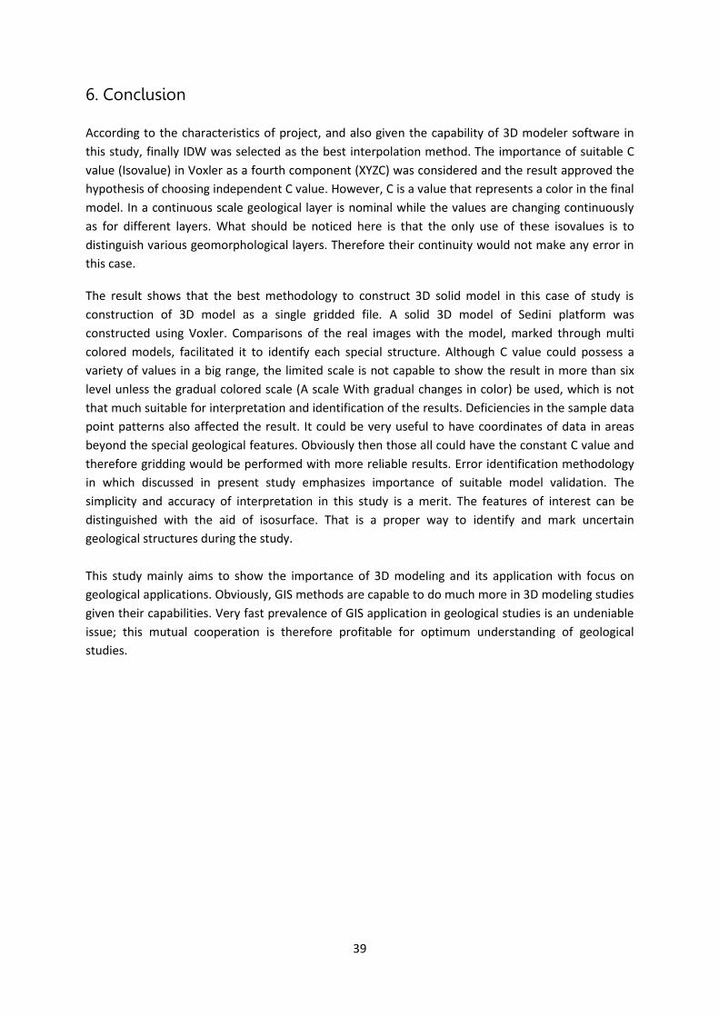
issue. Clip plane is a surface (plane) which can cut any area of the model in any direction. It can clip

where it should be observed behind the 3D surface. Movement of the clip plane in xyz equally,

results in 3D model shown in Figure 35 .The white line is in fact representation of the fissure and the

Black lines in two sides are geological boundaries.

According to the model, and given the values assigned to each feature in Table 6, the Black line at the

top of West side is 2e, while in the other side of the fissure we can see 2d. The 2nd line in the West

side shows 2d as Red colored but across it we have 2c as a Yellow layer. 3rd line in West side is 2c

Yellow colored, while 2b is located at border of Yellow and Green with value of 20-25. The last line in

the West is 2c again in border of Yellow and Green with value of 20-25. The interpretation justifies

the occurrence of fissure in the platform. However, some errors occur as well. In the West part of the

rift, there is continuation of boundary lines much longer than real instance. It is due to the

distribution of the data and interpolation result of these scattered data. However, it is an important

38

task to find the most suitable place to locate the clip plane. Integration of the scattered data can help

to choose suitable place of clip plane. At the same time, the comparison between the real image and

the model can help in finding the best place to locate the clipper.

Figure 34. Split in South view

Figure 35. Justification and interpretation of split in South view of 3D model

39

6. Conclusion According to the characteristics of project, and also given the capability of 3D modeler software in

this study, finally IDW was selected as the best interpolation method. The importance of suitable C

value (Isovalue) in Voxler as a fourth component (XYZC) was considered and the result approved the

hypothesis of choosing independent C value. However, C is a value that represents a color in the final

model. In a continuous scale geological layer is nominal while the values are changing continuously

as for different layers. What should be noticed here is that the only use of these isovalues is to

distinguish various geomorphological layers. Therefore their continuity would not make any error in

this case.

The result shows that the best methodology to construct 3D solid model in this case of study is

construction of 3D model as a single gridded file. A solid 3D model of Sedini platform was

constructed using Voxler. Comparisons of the real images with the model, marked through multi

colored models, facilitated it to identify each special structure. Although C value could possess a

variety of values in a big range, the limited scale is not capable to show the result in more than six

level unless the gradual colored scale (A scale With gradual changes in color) be used, which is not

that much suitable for interpretation and identification of the results. Deficiencies in the sample data

point patterns also affected the result. It could be very useful to have coordinates of data in areas

beyond the special geological features. Obviously then those all could have the constant C value and

therefore gridding would be performed with more reliable results. Error identification methodology

in which discussed in present study emphasizes importance of suitable model validation. The

simplicity and accuracy of interpretation in this study is a merit. The features of interest can be

distinguished with the aid of isosurface. That is a proper way to identify and mark uncertain

geological structures during the study.

This study mainly aims to show the importance of 3D modeling and its application with focus on

geological applications. Obviously, GIS methods are capable to do much more in 3D modeling studies

given their capabilities. Very fast prevalence of GIS application in geological studies is an undeniable

issue; this mutual cooperation is therefore profitable for optimum understanding of geological

studies.

40

References: Anonymous, 2006. GIS Dictionary, Kriging. [Online] Available at: http://support.esri.com/index.cfm?fa=knowledgebase.gisDictionary.search&searchTerm=kriging [Accessed July 2008]. Anonymous, Voxler knowledgebase questions. [Online]: http://www.goldensoftware.com/activekb/questions/383 [Accessed October 2008].

Benisek, M., Marcano, G., Mutti, M., Betzler, C., 2007. Coralline algal assemblages of a Burdigalian platform slope: implications for carbonate platform reconstruction (Northern Sardinia, Western Mediterranean sea). To be submitted for sedimentology and FACIES. Childs, C., 2004. Interpolating surfaces in ArcGIS spatial analyst, ESRI education services. Available at: http://www.esri.com/news/arcuser/0704/files/interpolating.pdf [Accessed June 2008]. Dangermond, J., 2006. An overview of GIS concepts, the Geodatabase, and the ArcGIS family of products .ESRI Electronic Book: http://www.esri.com/library/books/what-is-arcgis92.pdf [Accessed June 2008]. Geographical location of Sardinia. [Online] Available at: http://www.ercps.com/pasta/inf/reg/i/molise.gif [Accessed June 2008]. Gustavsson M., Seijmonsbergen A. and Kolstrup E., 2007. Structure and contents of a new geomorphologic GIS database linked to a geomorphologic map — with an example from Liden, central Sweden. Geomorphology, vol. 95. pp. 335–349. doi:10.1016/j.geomorph.2007.06.014. Ihrke, C., (n.d), Database Management and Spatial Interpolation of Geologic Boring Logs Using GIS at the Kalmar Landfill Rochester, MN. [Online] Available at: http://www.gis.smumn.edu/GradProjects/IhrkeC.pdf [Accessed June 2008]. Kaufmann, O., Thierry, M., 2007. 3D geological modeling from boreholes, cross-sections and geological maps, application over former natural gas storages in coal mines. Computers & Geosciences, Vol. 34. pp. 278–290. doi:10.1016/j.cageo.2007.09.005. Lu, G., Wong, D., 2007. An adaptive inverse-distance weighting spatial interpolation technique. Computers & Geosciences, Vol. 34. pp. 1044– 1055. doi:10.1016/j.cageo.2007.07.010. Merwade, V., Cook, A., Coonrod, J., 2008. GIS techniques for creating river terrain models for hydrodynamic modeling and flood inundation mapping. Environmental Modeling & Software, Vol. 23. Pp. 1300–1311. doi:10.1016/j.envsoft.2008.03.005. Spinosa, C., (n.d), Sardinia Geology [Online]. Boise State University, Department of Geosciences, Available at: http://earth.boisestate.edu/summercamp/geology.htm [Accessed 10 June 2008]. Tacher, L., Pomian-Srzednicki, I., Parriaux, A., 2006. Geological uncertainties associated with 3-D subsurface models. Computers & Geosciences. Vol. 32. pp212–221. doi:10.1016/j.cageo.2005.06.010. Yu, Z.W., 2000. Surface interpolation from irregularly distributed points using surface splines, with Fortran program. Computers & Geosciences.Vol. 27. pp 877–882. doi:10.1016/S0098-3004(01)00005-X. Zanchi, A., Francesca, S., Stefano, Z., Simone, S., Graziano, G., 2007. 3D reconstruction of complex geological bodies: Examples from the Alps. Computers & Geosciences.Vol. 35. pp 49-69. doi:10.1016/j.cageo.2007.09.003.

41

Zhou, W., Chen, G., Li, H., Luo, H., Huang, S., 2007. GIS application in mineral resource analysis—a case study of offshore marine placer gold at Nome. Computers & Geosciences, Vol. 33. pp 773–788. doi:10.1016/j.cageo.2006.11.001.