GRETHA UMR CNRS 5113 Université Montesquieu Bordeaux IV

Avenue Léon Duguit - 33608 PESSAC - FRANCE Tel : +33 (0)5.56.84.25.75 - Fax : +33 (0)5.56.84.86.47 - www.gretha.fr

Construction of linkage indicators of greenhouse gas emissions for

Aquitaine region

Jean-Christophe MARTIN

Patrick POINT

GREThA, CNRS, UMR 5113

Université de Bordeaux

Cahiers du GREThA

n° 2011-05

Cahiers du GREThA 2011 – 05

- 2 -

Construction d’indicateurs d’effets d’entrainement pour les émissions de gaz à effet de serre de la région Aquitaine

Résumé

Ce papier propose de construire des indicateurs d’effets d’entrainement sur les émissions de gaz à effet de serre (GES) dans la région Aquitaine en recourant à la notion d’intégration verticale avec une présentation du résultat sous forme de bloc. Du fait que la comptabilité régionale en France est peu développée, nous avons dû construire un tableau entrées-sorties (TES) pour la région Aquitaine avec un inventaire associé des émissions de GES. La méthode de construction du TES va influencer à la fois la fiabilité et la richesse des résultats.

Mots-clés : tableaux entrées-sorties régionalisés, quotients de localisation, émissions de gaz à effet de serre, indicateurs d’effets d’entrainement

Construction of linkage indicators of greenhouse gas emissions for Aquitaine region

Abstract

This paper proposes to construct linkage indicators of greenhouse gas (GHG) emissions for the Aquitaine region of France by using the notion of vertical integration with a presentation of results in the form of block. Because of poor regional accounting in France, we had to construct an input-output table for the Aquitaine region with a GHG emissions inventory associated. Method of construction of input-output table will affect both reliability and richness of results.

Keywords: regionalized input-output table, quotients of localization, greenhouse gas emissions, linkage indicators

JEL : C67, R15, E2, Q4, Q54

Reference to this paper: MARTIN Jean-Christophe, POINT Patrick, 2011, “Construction of linkage indicators of greenhouse gas emissions for Aquitaine region”, Cahiers du GREThA, n°2011-05, http://ideas.repec.org/p/grt/wpegrt/2011-05.html.

1 IntroductionIn order to fight against climate change, France has been committed to reduce its greenhousegas (GHG) emissions by four for 2050. The government is aware of some difficulties to reachits GHG emissions reduction target without an active participation of territorial collectivitiesand, particularly, of regions. The region of Aquitaine has implemented a climate plan in orderto avoid 2 883 ktCO2eq per year for 2007-2013, that is 13% of its GHG emissions of 2008. But,French regions need environmental studies in order to guide efficiently in the implementation oftheir climate plans.A policy against climate change needs to select main sectors having important linkages on re-gional GHG emissions. Input-output (IO) model is relevant for this issue because it incorporatesthe complexity of interindustrial trade with a detailed sectoral study (Leontief, 1986). Moreover,this model has been extended to environment (Leontief, 1970) and particularly to GHG emis-sions (Proops et al., 1993). Different research works show the interest of the IO modelling forenvironmental issues (Hawdon and Pearson, 1995 ; Zhang and Folmer, 1998 ; Munksgaard et al.,2005 ; Berck and Hoffman, 2002). Leontief model is a demand-driven model. So, emissions areentirely attributable to final demand (consumption-based accounting). This accounting methodenables to evaluate GHG emissions along the chains of production (Widermann, 2009). Themodel determines necessary direct and indirect GHG emissions to satisfy the final demand. Therediscovery of this analysis for regional studies in relation to the environment could be explainedfor different reasons. First, countries to respect their commitment taken in the Kyoto Protocolhave to implement climate plans at different geographical levels (international, national, regionaland local). Then, IO model is a good trade-off between the relevance of results and the specificregional constraints on data (West, 1995). We could cite for instance the work of Mc Gregor etal. (2008) concerning their studies on GHG emissions at regional level. Finally, the increasingpopularly of this model is explained by a more powerful capacity of computer to handle matrixinversion with large datasets (Loveridge, 2004). This model has some limitations because oflinearity assumption and no supply-side constraints (See Lenzen 2003, West 1995). However, thelinearity assumption enables to the model be tractable (Hawdon and Pearson, 1995).Three types of studies are possible thanks to IO analysis: to make descriptive studies, to con-tribute to impacts assessments and to construct some simulations. In this paper, we restrict toa descriptive study. We will evaluate both backward and forward GHG emissions of each sectorfor the Aquitaine region. We use the methodology of vertical integration presented by Pasinetti(1977) and developed by Duarte et al. (2002) and Sanchez-Choliz and Duarte (2003a, 2003b,2005). It is a relevant method for the studies on sectors interdependence. It overcomes the weak-nesses of Hirschman-Rasmussen indices (1958), highly used in literature (see Sanchez-Choliz andDuarte, 2003a). It has the interest to discriminate intersectoral demand with final demand bybreaking down GHG emissions of sectors on four components: net backward component, netforward component, internal component and mixed component. Although the authors used thismethodology for water study, this analysis could also be applied to GHG emissions study. Fur-thermore, Sanchez-Choliz and Duarte (2005) show the results in a sectors block enabling both asynthetic presentation of results and avoiding aggregation bias.But the carrying out of this study requires having an input-output table (IOT) with a GHGemissions inventory associated. However, as the national institute for statistics and economicstudies (INSEE) does not construct an IOT at regional level, we had to estimate one. In parallel,we construct a GHG emissions inventory consistent with the regional IOT nomenclature.We first explain the methodology of construction of IOT for the Aquitaine region with GHGemissions inventory associated. The construction of regional data will lead then to study the roleof sectors interdependence for regional GHG emissions.

1

2 presentation of technique of regionalizing national input-output table

Because of poor regional accounting in France, INSEE is not able to product an IOT at regionallevel. We had so to estimate one. We will explain the main steps to construct a regional IOT.

2.1 Adoption of top-down approachThe construction of IOT for the Aquitaine region must fulfil a double requirement: costlessin time and in human resources, and errors from the hypotheses of construction will influencemoderately the results of the model though it is difficult to quantify them. Therefore, themethodologies that we will adopt must fulfil these different requirements because the construc-tion of this regional IOT is only a step for environmental studies.Two traditional methods exist to construct regional IOT: "bottom-up method" and "top-down"method. The first method uses directly regional data thanks to surveys and interviews whereasthe second method consists of regionalizing national IOT using statistical indicators.From the theoretical point of view, the first method is preferable because it enables to incorpo-rate well regional specificities. The techniques of production are differentiated between regions.A specific nomenclature is elaborated in order to take account regional productive structure. InUSA, one of the most famous examples is the construction of IOT for the State of Washingtonfor the following years 1963, 1969, 1972, 1982 and 1987 by Chase, Bourque and Conway (1993).Although the Anglo-Saxon literature is scarce, it does not exclude interesting experiences onforeign countries, rarely writing in English language (Boomsma and Oosterhaven, 1992). Forinstance, in Spain, the regional institutes for statistics have constructed IOT based on surveys.Cortinas and Vicente (2009) show the method of construction of IOT for Castilla la mancha,one of Spanish provinces. The construction of regional IOT in France by bottom-up method wasintroduced by Bauchet for the Lorraine region in 1955. After, each French region was concernedby this work between 1955 and 1970. Concerning the Aquitaine region, we could cite the works ofprofessor Jouandet-Bernadat (1965) thanks to the help of members of the institute of the regionaleconomics of South-West (IERSO). But, the constitution of regional IOT was often incompletebecause these IOT were more devoted to study the regional productive structure than to makeforecasting and simulation studies by using input-output analysis (Ousset J, 1975).The relatively low use of this method comparatively to top-down method is explained by itsdifferent limitations. Richardson (1972) explains them. First, survey requires obtaining complexinformation. Then, the response rates are very low. Finally, there are the dangers to obtainincorrect information. Because of these different difficulties, adjustments processes are so nec-essary to implement in order to verify supply-use equilibrium of products. This work is costlybecause it needs considerable financial and human resources. It is a research project carriedout by a research institute or a research team. Mattas et al. (1984) estimate that cost for theconstruction of the IOT by "bottom-up" method are twenty higher than "top-down" method."Top-down" method is more relevant for this issue. It aims to regionalize at lower cost the differ-ent national input-output components by using available statistical indicators. It avoids inherentdifficulties of surveys. This method is largely explained in Miller and Blair (1985).This modelassumes that production techniques are relatively stable within a nation. Importations enablingto calculate regional technical coefficients are estimated by location quotients, which a lot ofresearch in regional economics are focus on. Miller and Blair (1985) indicated the main locationquotients1 . Recently, some improvements could be made for "weighted" location quotients (Flegg

1simple location quotient, purchases-only location quotients, cross-industry quotients, supply-demand poolapproaches, fabrication effects and regional purchase coefficients

2

and webber, 1997). Literature about the construction of regional IOT with top-down methoddeveloped by Isard (1951) is more abundant because it enables to construct rapidly and at leastcost. Since 1970, the Bureau of Economic Analysis (BEA) has developed a methodology to es-timate regional multipliers, named RIMS (Regional Input-output Modelling System). RegionalIOT are estimated from national IOT, which are then adjusted thanks to regional data enablingto integrate some regional specificities. The RIMES model is currently used in USA to assessimpacts of a project at regional level. In France, one of the most famous works comes from Cour-bis and Pommier (1979) thanks to the team of researchers at the laboratory of GAMA. Francewas divided into five big regions where an IOT for each region was constructed thanks to manydifferent statistical data of INSEE. These regional IOT were consistent with the national IOT:the sum of these regional IOT constitutes the national IOT. They built a very developed andrigorous methodology in order to regionalize national IOT. This work was involving an importantmobilization of members of the laboratory of GAMA during four years (from 1972 to 1976). Theconstruction of regional IOT constituted the basis of REGINA model, with an objective to studynational-regional interactions. Concerning the Aquitaine region, Delfaud (1982) built an IOT bytop-down method in order to make some forecasting studies by using input-output analysis.This method has also some limitations because of weak theoretical base (Brand, 1997) and noincorporation of regional specificities. The production function is considered to be homogeneouswithin a nation (Jouandet-Bernadat, 1967). But this construction method has the interest tobe rapid, coherent and operational to an input-output analysis. In order to incorporate betterregional specificity, we used some surveys made by the national institute for statistics.However, the regionalization of a national IOT requires that the national IOT is symmetric andexpressed entirely at basic price in order to be compatible with an input-output analysis. Thisstep will enable then to regionalize national IOT for the Aquitaine region.

2.2 The construction of a symmetric national input-output tableThe starting point is the national IOT for 2001 in 114 sectors. It is highly recommended to re-gionalize the most disaggregated national IOT in order avoid the famous problem of aggregationbias (Malinvaud, 1954).The national IOT as presented by INSEE is not operational to input-output analysis becauseIOT in 114 sectors is a commodity-by-industry input-output account. INSEE does not estimatea symmetric IOT at this level of aggregation. Furthermore, INSEE doest not discriminate the(domestic and imported) origin of products for the demand of the product and they are entirelyexpressed in purchasers’ prices. We indicate the three steps necessary to construct a symmetricnational IOT.The first step consists of evaluating intermediate and final demand at basic price. The databaseNOUBA indicates for each component of intermediate and final demand trade margins, trans-portation margins and taxes for 2002, but not for 2001. We assumed that the share of marginsin intermediate and final demand is identical for 2001 and 2002. As soon as we estimated thesemargins, we reallocated them into the concerned products according to recommendations ofMiller and Blair (1985). Transport margins will so be allocated to transport products and trademargins to trade products. We must then subtract taxes. INSEE indicates also for each compo-nents of intermediate and final demand the amount of taxes by assuming the share of taxes onintermediate demand is identical. We obtain so an interindustrial transactions table expressed atbasic price. But the interindustrial transactions table is still a "commodity-by-industry" matrix.The second step consists of transforming "commodity-by-industry" transactions table into "commodity-by-commodity" transactions table. Input-output analysis requires to construct a "commodity-by-commodity" transactions table (Miller and Blair, 1985). To make this matrix, two assumptions

3

are possible: the commodity technology assumption or industry technology assumption (TenRaa and Rueda-Cantuche, 2007). The commodity technology assumption argues that industrieshave the same input structure. On contrary, industry technology assumption argues that com-modities have the same input structure. The commodity technology assumption is preferablefrom an axiomatic point of view (Jansen and Ten Raa,1990) but it implies negative technicalcoefficients. Some methods have been developed to solve this problem (Almon, 2000). Thisassumption is the most used (Eurostat 2008, Bohlin and Widell, 2006). On contrary, the indus-try technology assumption has the interest to avoid negative technical coefficients (De Mesnard,2004a) ant it is more coherent with a circuit approach (De Mesnard, 2004b). This assumptionhas been selected for the construction of French symmetric IOT (Braibant, 2006) and for someother IOT (Fritz et al., 2003). We followed the recommendations of De Mesnard (2004b) andBraibant (2006) with a construction of a commodity-by-commodity national IOT by using theindustry technology assumption. A supply matrix is essential to make this transformation. Toobtain a commodity-by-commodity transaction table, it is sufficient to multiply the commodity-by-industry transaction table by the transpose of the supply matrix expressed in percentage.The value added is also calculated by using the supply matrix. We obtain so a symmetric input-output table, expressed entirely to basic price.The third step consists of discriminating domestic and imported origins for intermediate and finaldemand. This step is crucial to compute national technical coefficients. This result will use afterto compute regional technical coefficients. INSEE accounts the importations of products when itcomes into the national territory by the customs services without worrying about the destinationof products. INSEE makes some estimation about the destination of imported products but theyare not willing to communicate it because of too many uncertainties in their results. Because ofnot sufficient statistical data, importation will be allocated to intermediate and final demandson the basis of output coefficients. This assumption implies that the share of imported productsof each components of intermediate and final demand is identical for each sector.After making these different calculations, we could obtain a national symmetric commodity-by-commodity transaction table, operational to an input-output analysis. We must now regionalizedifferent components of the national IOT.

2.3 Estimation of regional added valueINSEE estimates the added values at regional level with a high level of aggregation (14 sectors).It is essential to estimate these added values in more disaggregated level, that is in 114 sectors.The estimated values from INSEE will be served to quantify errors estimations.A Traditional way to estimate the added value is to use top-down method by assuming thatthe labour productivity of each sector is similar whatever the geographical level within a nation(Schaffer and Chu, 1969 ; Kronenberg, 2009). The regional added value is calculated by makingthe ratio of national added value to national employed people in sectors i that we multiply thenby regional employed people in this sector. However, this calculation requires data on employedpeople by sector at regional level. In France, there are two available datasets indicating thenumber of employed people by sector: the population census and data from UNEDIC2 (L’UnionNationale interprofessionnelle pour l’Emploi Dans l’Industrie et le Commerce).The first dataset is the most exhaustive because it is a result of compulsory survey for nationalpopulation. But it is taken every 7 years. The population census closest to 2001 is 1999. Thesecond dataset is taken every year. It accounts the number of salary with a detailed geographicalarea. But are excluded salaried employee of State and territorial collectivities, employee ofembassy, foreign consulate and international organization, salaried employee of farm sectors,

2the institution that manages the funds of the "Assurance ch?mage" and that pays unemployment benefits

4

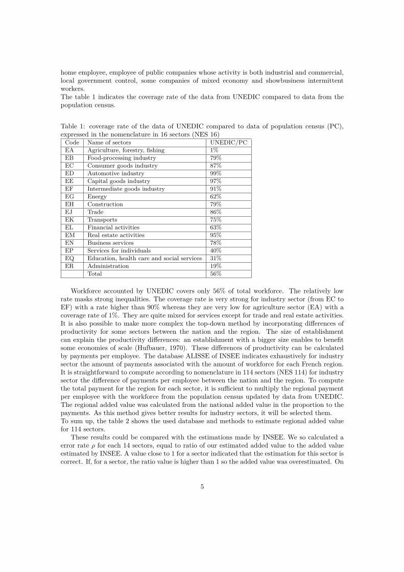
home employee, employee of public companies whose activity is both industrial and commercial,local government control, some companies of mixed economy and showbusiness intermittentworkers.The table 1 indicates the coverage rate of the data from UNEDIC compared to data from thepopulation census.

Table 1: coverage rate of the data of UNEDIC compared to data of population census (PC),expressed in the nomenclature in 16 sectors (NES 16)Code Name of sectors UNEDIC/PCEA Agriculture, forestry, fishing 1%EB Food-processing industry 79%EC Consumer goods industry 87%ED Automotive industry 99%EE Capital goods industry 97%EF Intermediate goods industry 91%EG Energy 62%EH Construction 79%EJ Trade 86%EK Transports 75%EL Financial activities 63%EM Real estate activities 95%EN Business services 78%EP Services for individuals 40%EQ Education, health care and social services 31%ER Administration 19%

Total 56%

Workforce accounted by UNEDIC covers only 56% of total workforce. The relatively lowrate masks strong inequalities. The coverage rate is very strong for industry sector (from EC toEF) with a rate higher than 90% whereas they are very low for agriculture sector (EA) with acoverage rate of 1%. They are quite mixed for services except for trade and real estate activities.It is also possible to make more complex the top-down method by incorporating differences ofproductivity for some sectors between the nation and the region. The size of establishmentcan explain the productivity differences: an establishment with a bigger size enables to benefitsome economies of scale (Hufbauer, 1970). These differences of productivity can be calculatedby payments per employee. The database ALISSE of INSEE indicates exhaustively for industrysector the amount of payments associated with the amount of workforce for each French region.It is straightforward to compute according to nomenclature in 114 sectors (NES 114) for industrysector the difference of payments per employee between the nation and the region. To computethe total payment for the region for each sector, it is sufficient to multiply the regional paymentper employee with the workforce from the population census updated by data from UNEDIC.The regional added value was calculated from the national added value in the proportion to thepayments. As this method gives better results for industry sectors, it will be selected them.To sum up, the table 2 shows the used database and methods to estimate regional added valuefor 114 sectors.

These results could be compared with the estimations made by INSEE. We so calculated aerror rate ρ for each 14 sectors, equal to ratio of our estimated added value to the added valueestimated by INSEE. A value close to 1 for a sector indicated that the estimation for this sector iscorrect. If, for a sector, the ratio value is higher than 1 so the added value was overestimated. On

5

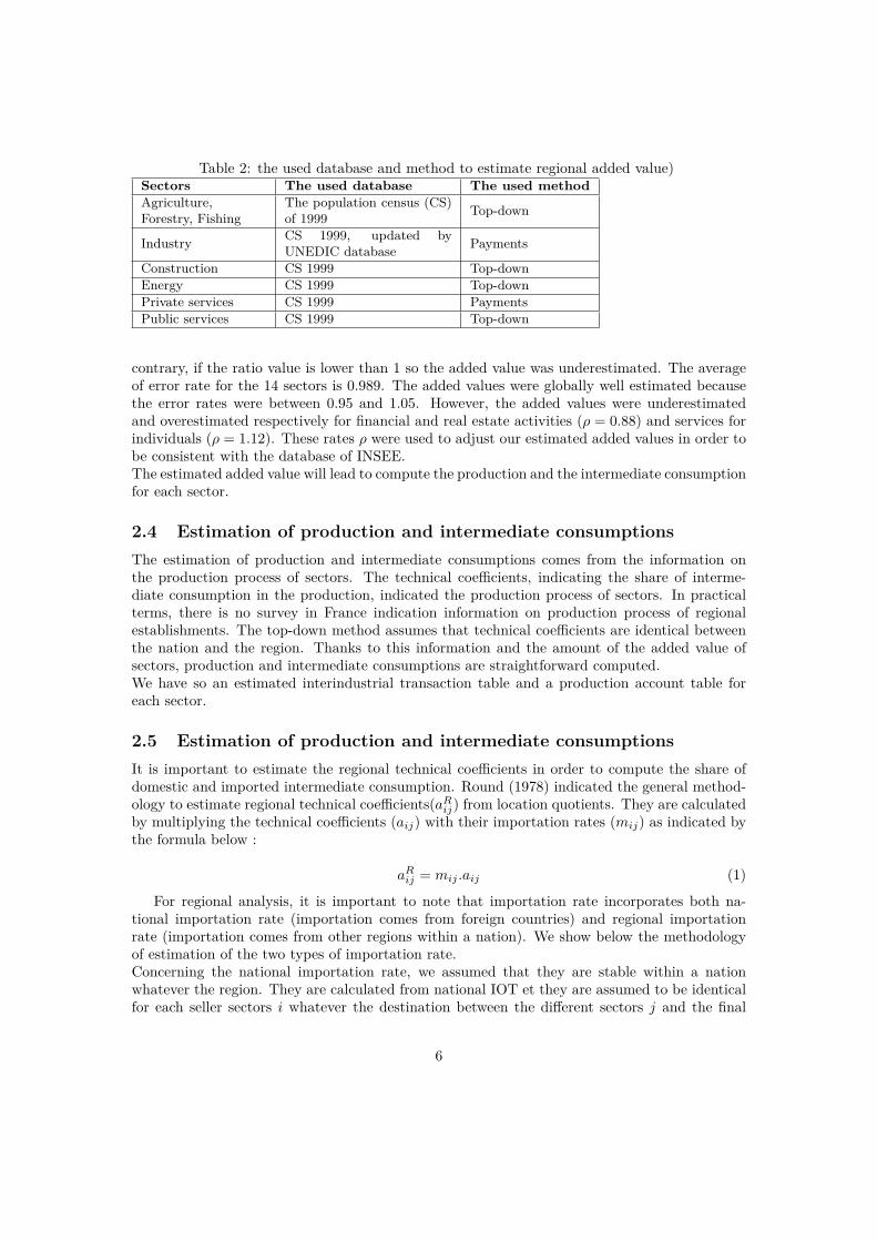
Table 2: the used database and method to estimate regional added value)Sectors The used database The used methodAgriculture,Forestry, Fishing

The population census (CS)of 1999 Top-down

Industry CS 1999, updated byUNEDIC database Payments

Construction CS 1999 Top-downEnergy CS 1999 Top-downPrivate services CS 1999 PaymentsPublic services CS 1999 Top-down

contrary, if the ratio value is lower than 1 so the added value was underestimated. The averageof error rate for the 14 sectors is 0.989. The added values were globally well estimated becausethe error rates were between 0.95 and 1.05. However, the added values were underestimatedand overestimated respectively for financial and real estate activities (ρ = 0.88) and services forindividuals (ρ = 1.12). These rates ρ were used to adjust our estimated added values in order tobe consistent with the database of INSEE.The estimated added value will lead to compute the production and the intermediate consumptionfor each sector.

2.4 Estimation of production and intermediate consumptionsThe estimation of production and intermediate consumptions comes from the information onthe production process of sectors. The technical coefficients, indicating the share of interme-diate consumption in the production, indicated the production process of sectors. In practicalterms, there is no survey in France indication information on production process of regionalestablishments. The top-down method assumes that technical coefficients are identical betweenthe nation and the region. Thanks to this information and the amount of the added value ofsectors, production and intermediate consumptions are straightforward computed.We have so an estimated interindustrial transaction table and a production account table foreach sector.

2.5 Estimation of production and intermediate consumptionsIt is important to estimate the regional technical coefficients in order to compute the share ofdomestic and imported intermediate consumption. Round (1978) indicated the general method-ology to estimate regional technical coefficients(aRij) from location quotients. They are calculatedby multiplying the technical coefficients (aij) with their importation rates (mij) as indicated bythe formula below :

aRij = mij .aij (1)

For regional analysis, it is important to note that importation rate incorporates both na-tional importation rate (importation comes from foreign countries) and regional importationrate (importation comes from other regions within a nation). We show below the methodologyof estimation of the two types of importation rate.Concerning the national importation rate, we assumed that they are stable within a nationwhatever the region. They are calculated from national IOT et they are assumed to be identicalfor each seller sectors i whatever the destination between the different sectors j and the final

6

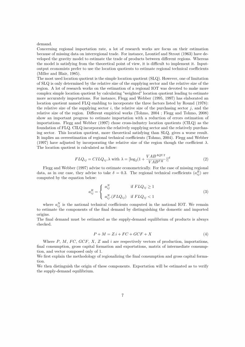
demand.Concerning regional importation rate, a lot of research works are focus on their estimationbecause of missing data on interregional trade. For instance, Leontief and Strout (1963) have de-veloped the gravity model to estimate the trade of products between different regions. Whereasthe model is satisfying from the theoretical point of view, it is difficult to implement it. Input-output economists prefer to use the location quotients to estimate regional technical coefficients(Miller and Blair, 1985).The most used location quotient is the simple location quotient (SLQ). However, one of limitationof SLQ is only determined by the relative size of the supplying sector and the relative size of theregion. A lot of research works on the estimation of a regional IOT was devoted to make morecomplex simple location quotient by calculating "weighted" location quotient leading to estimatemore accurately importations. For instance, Flegg and Webber (1995, 1997) has elaborated anlocation quotient named FLQ enabling to incorporate the three factors listed by Round (1978):the relative size of the supplying sector i, the relative size of the purchasing sector j, and therelative size of the region. Different empirical works (Tohmo, 2004 ; Flegg and Tohmo, 2008)show an important progress to estimate importation with a reduction of errors estimation ofimportations. Flegg and Webber (1997) chose cross-industry location quotients (CILQ) as thefoundation of FLQ. CILQ incorporates the relatively supplying sector and the relatively purchas-ing sector. This location quotient, more theoretical satisfying than SLQ, gives a worse result.It implies an overestimation of regional technical coefficients (Tohmo, 2004). Flegg and Webber(1997) have adjusted by incorporating the relative size of the region though the coefficient λ.The location quotient is calculated as follow:

FLQij = CILQij .λ with λ = [log2(1 + V ABAQUI

V ABFR)]δ (2)

Flegg and Webber (1997) advise to estimate econometrically. For the case of missing regionaldata, as in our case, they advise to take δ = 0.3. The regional technical coefficients (aRij) arecomputed by the equation below:

aRij =

aNij if FLQij ≥ 1

aNij .(FLQij) if FLQij < 1(3)

where aNij is the national technical coefficients computed in the national IOT. We remainto estimate the components of the final demand by distinguishing the domestic and importedorigins.The final demand must be estimated as the supply-demand equilibrium of products is alwayschecked.

P +M = Z.i+ FC +GCF +X (4)

Where P , M , FC, GCF , X, Z and i are respectively vectors of production, importations,final consumption, gross capital formation and exportations, matrix of intermediate consump-tion, and vector composed only of 1.We first explain the methodology of regionalizing the final consumption and gross capital forma-tion.We then distinguish the origin of these components. Exportation will be estimated as to verifythe supply-demand equilibrium.

7

2.6 The final consumptionIt is important to distinguish the final consumption of households, government and non-profitinstitutions serving households.Concerning the final consumption of households, we first assume that consumption per headis identical within a nation for each product. The consumption per head is calculated by theratio of final consumption of products indicated in the national IOT to the French population.The final consumption of products of regional IOT is found by multiplying these ratios with theregional population. We then integrate some regional specificity concerning the consumption perhead by taken again the methodology of Courbis (1979). The consumption per head could beregionalized thanks to the survey of family budget indicating the consumption of 195 products for8 geographical areas. We have to adjust the nomenclature of this survey with the nomenclaturefor 114 sectors used by the national IOT.Concerning the final consumption of government, we must distinguish the individual and collec-tive consumptions. Concerning the individual consumption, it was possible to incorporate someregional specificity by using some regional databases indicated in the table below

Table 3: Databases used to regionalize the individual final consumption of governmentSectors Database Source of databasePharmaceuticalproducts Number of pharmacists Directory of research, studies, eval-

uation and statistics (DREES)Education Number of pupils and students Ministry of Education

Health care Number of professional in thehealth care DREES

Social services Available number of places to re-ceive disable people DREES

Concerning the collective final consumption of government, we assumed that services of States(Justice, Defence,. . . ) are equitably distributed to the population without geographical discrim-ination.Concerning the final consumption of non-profit institutions serving households, we regionalizedthe consumption in proportion to the population by assuming that the consumption per head isidentical between the regions within the nation.

2.7 The gross capital formationWe have now to estimate the gross capital formation. The different surveys concerning theinvestments of firms (SESSI database) indicate only the buying of investment goods, but not theselling of investment goods. As we could not obtain the capital matrix indicating the investmentgoods flow, it was not possible to regionalize it and so to incorporate some regional specificities.Because of statistical constraints, we had to assume that the share of investment goods productsby the sector is identical between the nation and the region . We have so an estimation of regionaldemand for investment goods.

2.8 Estimation of domestic and imported components of final demand(except exportation)

It is important for the construction of our model to distinguish the domestic and import sharesof final demand components. The supply-demand equilibrium of regional products is describedby the equation below:

8

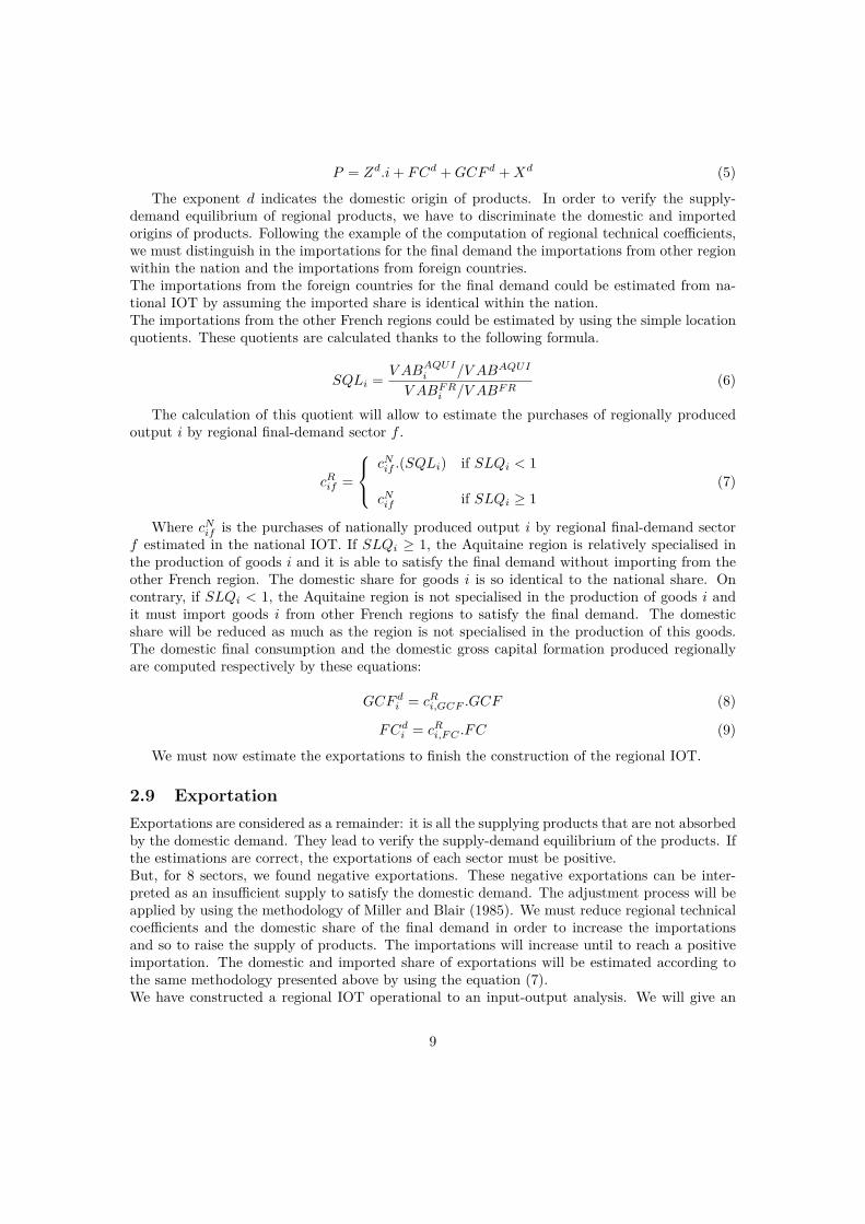
P = Zd.i+ FCd +GCF d +Xd (5)

The exponent d indicates the domestic origin of products. In order to verify the supply-demand equilibrium of regional products, we have to discriminate the domestic and importedorigins of products. Following the example of the computation of regional technical coefficients,we must distinguish in the importations for the final demand the importations from other regionwithin the nation and the importations from foreign countries.The importations from the foreign countries for the final demand could be estimated from na-tional IOT by assuming the imported share is identical within the nation.The importations from the other French regions could be estimated by using the simple locationquotients. These quotients are calculated thanks to the following formula.

SQLi = V ABAQUIi /V ABAQUI

V ABFRi /V ABFR(6)

The calculation of this quotient will allow to estimate the purchases of regionally producedoutput i by regional final-demand sector f .

cRif =

cNif .(SQLi) if SLQi < 1

cNif if SLQi ≥ 1(7)

Where cNif is the purchases of nationally produced output i by regional final-demand sectorf estimated in the national IOT. If SLQi ≥ 1, the Aquitaine region is relatively specialised inthe production of goods i and it is able to satisfy the final demand without importing from theother French region. The domestic share for goods i is so identical to the national share. Oncontrary, if SLQi < 1, the Aquitaine region is not specialised in the production of goods i andit must import goods i from other French regions to satisfy the final demand. The domesticshare will be reduced as much as the region is not specialised in the production of this goods.The domestic final consumption and the domestic gross capital formation produced regionallyare computed respectively by these equations:

GCF di = cRi,GCF .GCF (8)

FCdi = cRi,FC .FC (9)

We must now estimate the exportations to finish the construction of the regional IOT.

2.9 ExportationExportations are considered as a remainder: it is all the supplying products that are not absorbedby the domestic demand. They lead to verify the supply-demand equilibrium of the products. Ifthe estimations are correct, the exportations of each sector must be positive.But, for 8 sectors, we found negative exportations. These negative exportations can be inter-preted as an insufficient supply to satisfy the domestic demand. The adjustment process will beapplied by using the methodology of Miller and Blair (1985). We must reduce regional technicalcoefficients and the domestic share of the final demand in order to increase the importationsand so to raise the supply of products. The importations will increase until to reach a positiveimportation. The domestic and imported share of exportations will be estimated according tothe same methodology presented above by using the equation (7).We have constructed a regional IOT operational to an input-output analysis. We will give an

9

example of the using of this IOT by estimating linkage indicators of GHG emissions of differentblocks for the Aquitaine region for 2001.

3 Linkage indicators of greenhouse gas emissionsWe must first present the GHG emissions function by indicating rapidly the methodology of theconstruction of GHG emissions inventory associated with the regional IOT. The work will enableus to compute the linkage indicators to estimate the buying and the selling of GHG emissionsincorporating in the regional products of each block.

3.1 Construction of the GHG emissions functionThe construction of GHG emissions function implies to make before a GHG emissions inventory.For this study, we consider three GHG: carbon dioxide (CO2), methane (CH4) and nitrousoxide (N2O). The Kyoto protocol accounts also three other GHG but they are not incorporatedin this study because of difficulties to estimate them and a low contribution to total GHGemissions (3%). GHG emissions come from as well as the production process than the householdconsumption for the fossil fuels. We considered in this paper only GHG emissions from theproduction process because the aim of this study is to explain GHG emissions of sectors dependingon the structure of the regional interindustrial trade.For this case, GHG emissions come from two sources (Proops et al. 1993)

• Combustion of fossil fuels: the carbon integrated in the fossil fuel is released back in theatmosphere as carbon dioxide during its combustion. The burning of fossil fuels can alsoemit methane and nitrous oxide.

• Specific to production process: It is all GHG emissions that could not be explained by theburning of fossil fuels but they are generated by a specific production process (carbonaceousclays, fermentation, outflows of gas fuel transport, waste deterioration, . . . ).

The construction of GHG emissions inventory was carried out in accordance with the method-ology of the CITEPA (Centre Interprofessionnel Techniques des Etudes de la Pollution Atmo-sphérique) and the recommendation of intergovernmental panel on climate change (IPCC). Thedocument OMINEA (methods for the construction of national inventories for atmospheric pol-lutions for France) indicates the GHG emissions coefficients for each fossil fuel. We aggregatedthen these fossil fuels into four categories: solid fuels (from coal), liquid fuels (from crude oil),gas fuels (from natural gas) and wood. A special feature was made to account GHG emissionsfrom wood. We assumed that CO2 emissions from the cutting of trees are offset by the car-bon sequestration from reforestation. Each trees cut is automatically replanted. So, the carbonfootprint is assumed to be zero. However, CH4 and N2O emissions from wood combustion areaccounted because it is a result of incomplete combustion. Our GHG emissions inventory wasconstructed in concordance with the GHG emissions inventory for the Aquitaine region madeby the CITEPA for the French Environment and Energy Management Agency (ADEME). GHGemissions can be related to production according to the formula below:

E = (e′c+m′)P (10)

WhereP is the n-vector of productionm is the n-vector of GHG emissions coefficients indicating necessary GHG emissions from specific

10

production processes (in tCO2eq) to produce one euro.c is the n-vector of energy intensity indicating necessary energy consumption (in tonne of oilequivalent or toe) to produce one euro.e is the n-vector of GHG emissions coefficients indicating GHG emissions resulting of a burningof one toe of fossil fuels.The apostrophe and the circumflex accent mean respectively the matrix transpose and the di-agonal matrix. The letter n indicates the number of sectors. To simplify the notation, we putk′ = (e′c+m′) where the vector k means total GHG emissions to produce one euroThis formula requires to link economic data with environmental data. However, these differentdata are expressed in different nomenclatures: NES for economic data, nomenclature of energyconsumption (NCE) for energy data and common report format (CRF) for GHG emissions data.A specific nomenclature was created to link these different nomenclatures. This work leads to anomenclature with 47 sectors that it is able to see in annex. GHG emissions function has beenconstructed enabling to compute linkage indicators.

3.2 The linkage indicatorsThe linkage indicators rely on the Leontief model enabling to incorporate the complexity of in-terindustrial trade for a region. The supply-demand equilibrium of domestic products indicatesthat the regional production is equal to the sum of the intermediate demand (used for interme-diate consumption of sectors) and the final demand of domestic products.The Leontief model, thanks to the assumption of the stability of the technical coefficients, calcu-lates direct and indirect production (for backward sectors) to satisfy the final demand. Technicalcoefficients are defined as necessary inputs to produce one euro. For regional studies, it is bet-ter to use regional technical coefficients (Miller and Blair, 1985) because it indicated necessaryregional inputs to produce one euro of regional product. The production function for a regionaleconomy is written as below:

P = AR.P + Y d (11)

WhereP is the n-vector of productionAR is the (n× n) matrix of regional technical coefficients.Y d is the n-vector of final demand for regional products.Equation (11), after rearrangement, can also be written as below:

P = (I −AR)−1.Y d (12)

Where (I−AR)−1 is the inverse matrix of Leontief. It indicates necessary direct and indirectregional production to satisfy one euro of final demand of a regional product. It is possible toextend this model to GHG emissions by integrating (10) into (12):

E = k′.(I −AR)−1.Y d (13)

Where k′.(I − AR)−1 is direct and indirect regional GHG emissions to satisfy one euro offinal demand for a regional product.As we have a large number of sectors (47 sectors), it is difficult to show the results with a solarge number of sectors. We use the blocks notion presented by Sanchez and Duarte (2005). Theblocks have the interest to show the results in an aggregated way by avoiding the aggregationbias.Considering Bs a block of sectors of the economy and B−S the remaining sectors. Thanks to

11

the blocks system and by using the equation (11), the production function can also be writtenas follow: (

PSP−S

)=(ARS,S ARS,−SAR−S,S AR−S,−S

)(PSP−S

)+(Y dSY d−S

)(14)

Equation (14), after rearrangement, can also be written as:(PSP−S

)=(

∆RS,S ∆R

S,−S∆R−S,S ∆R

−S,−S

)(Y dSY d−S

)(15)

Where (I −AR)−1 =(

∆RS,S ∆R

S,−S∆R−S,S ∆R

−S,−S

)with ∆R

S,S ≥ (I −AS,S)−1 and

∆R−S,−S ≥ (I −A−S,−S)−1

It is also possible to extend equation (15) to GHG emissions.(ESE−S

)=(kS 00 k−S

)(∆RS,S ∆R

S,−S∆R−S,S ∆R

−S,−S

)(Y dSY d−S

)(16)

Thanks to equations (12) and (16), it is possible to discriminate GHG emissions depending onfour effects for each block:

• internal effect: k′S(I −ARS,S)−1Y dS

• mixed effect: k′S [∆RS,S − (I −ARS,S)−1]Y dS

• net backward effect: k′−S∆R−S,S .Y

dS

• net forward effect: k′S∆RS,−S .Y

d−S

The internal effect indicates emissions produced by the block BS that are never integratedinto the production of goods of the block B−S . The mixed effect is the emissions from theproduction of goods BS that are incorporated into the production process as input for the blockB−S and come back to BS to satisfy the final demand. The net backward effect represents thenet buying of GHG emissions: it is all GHG emissions from the production of block B−S usedas input for the production of BS in order to satisfy the final demand without coming back tothe initial block. The net forward effect represents the net selling GHG emissions: it is all GHGemissions from the production of BS and used as input for the production of B−S in order tosatisfy the final demand without coming back to the initial block.These different effects will able to calculate both direct and embodied GHG emissions. DirectGHG emissions are composed of all emissions from the production of BS whatever it satisfiesthe final demand of BS than B−S . They are calculating by summing the internal, mixed andnet forward effects. They indicate the sector contribution for regional GHG emissions. Oncontrary, embodied GHG emissions of BS represents all GHG emissions from direct and indirectproduction to satisfy the final demand of BS . They are calculating by summing the internal,mixed and backward effects. The indicated the responsibility of final demand of block BS forregional GHG emissions.Block BS is a net seller of GHG emissions if its direct GHG emissions are higher than theirembodied GHG emissions. On contrary, block BS is a net buyer of GHG emissions if theirembodied GHG emissions are higher than their direct GHG emissions.

12

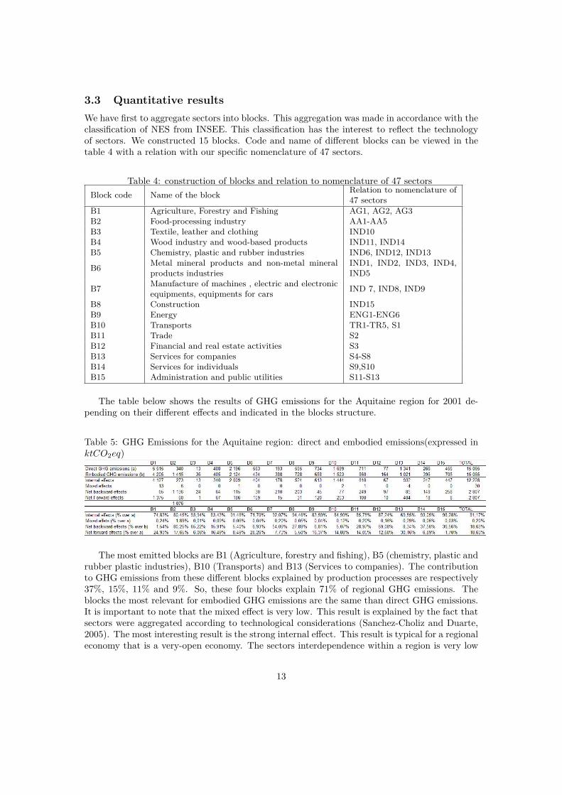
3.3 Quantitative resultsWe have first to aggregate sectors into blocks. This aggregation was made in accordance with theclassification of NES from INSEE. This classification has the interest to reflect the technologyof sectors. We constructed 15 blocks. Code and name of different blocks can be viewed in thetable 4 with a relation with our specific nomenclature of 47 sectors.

Table 4: construction of blocks and relation to nomenclature of 47 sectorsBlock code Name of the block Relation to nomenclature of

47 sectorsB1 Agriculture, Forestry and Fishing AG1, AG2, AG3B2 Food-processing industry AA1-AA5B3 Textile, leather and clothing IND10B4 Wood industry and wood-based products IND11, IND14B5 Chemistry, plastic and rubber industries IND6, IND12, IND13

B6 Metal mineral products and non-metal mineralproducts industries

IND1, IND2, IND3, IND4,IND5

B7 Manufacture of machines , electric and electronicequipments, equipments for cars IND 7, IND8, IND9

B8 Construction IND15B9 Energy ENG1-ENG6B10 Transports TR1-TR5, S1B11 Trade S2B12 Financial and real estate activities S3B13 Services for companies S4-S8B14 Services for individuals S9,S10B15 Administration and public utilities S11-S13

The table below shows the results of GHG emissions for the Aquitaine region for 2001 de-pending on their different effects and indicated in the blocks structure.

Table 5: GHG Emissions for the Aquitaine region: direct and embodied emissions(expressed inktCO2eq)

The most emitted blocks are B1 (Agriculture, forestry and fishing), B5 (chemistry, plastic andrubber plastic industries), B10 (Transports) and B13 (Services to companies). The contributionto GHG emissions from these different blocks explained by production processes are respectively37%, 15%, 11% and 9%. So, these four blocks explain 71% of regional GHG emissions. Theblocks the most relevant for embodied GHG emissions are the same than direct GHG emissions.It is important to note that the mixed effect is very low. This result is explained by the fact thatsectors were aggregated according to technological considerations (Sanchez-Choliz and Duarte,2005). The most interesting result is the strong internal effect. This result is typical for a regionaleconomy that is a very-open economy. The sectors interdependence within a region is very low

13

because of strong importation and exportation.The advantage to distinguish the net backward effect and the net forward effect is to select themost net buyer and net seller blocks of GHG emissions. A net buyer block of GHG emissionsis selected by greater net backward effect than net forward effect, implying that direct GHGemissions are lower than integrated GHG emissions. The biggest buyers of GHG emissions areB2, B15 and B7. The net buying 3 of GHG emissions of these respectively blocks are 1,076ktCO2eq, 250 ktCO2eq and 195 ktCO2eq. The share of net backward effect is respectively 50%,37% and 54%. It is interesting to note that blocks B3 and B12 have important net backwardeffect with respectively rates of 65% and 59%.The net seller blocks of GHG emissions are B1 and B13. The net selling 4 of GHG emissions forthese blocks is respectively 1310 ktCO2eq and 319 ktCO2eq. The share of net forward effect isrespectively to 25% and 30%. It is interesting to note that block B6 has an important forwardeffect with a rate of 28%.It is possible to detail information from table 5 by breaking down GHG emissions from netbackward and net forward effects between different blocks that you could see on table 6.

Table 6: Breakdown of regional GHG emissions by block (in ktCO2eq)

The emissions in column indicate the selling of emissions for the final demand of each block.For instance, the block B1 sold 4,140 ktCO2eq to its final demand, 1,040 ktCO2eq to B2, 6ktCO2eq to B3, and so on. The selling of emissions at the block itself corresponds to mixed andinternal effects. So, the sum of GHG emissions in column corresponds to direct emissions. Oncontrary, the emissions in rows indicate the buying of emissions by a block from different blocksto satisfy its final demand. The final demand of block B1 implied emissions of 4,140 ktCO2eqto B1, 24 ktCO2eq to B2, 0 ktCO2eq to B3, and so on. The buying of emissions from the finaldemand to the same block corresponds to the sum of mixed and internal effects whereas the sumof emissions of final demand to other blocks corresponds to net backward effect. So, the sum ofemissions in row indicates embodied emissions.The table allows us to select the most important trade of regional GHG emissions between blocks.It is interesting to note that the most important trade of GHG emissions comes from the sellingfrom B1 to B2 (1,040 ktCO2eq), B11 (82 ktCO2eq), B14 (69 ktCO2eq). Moreover, the block B8buys GHG emissions with B6 (72 ktCO2eq), as well as B15 with B13 (78 ktCO2eq) and B13with B11 (60 ktCO2eq).Vertical reading indicates the breakdown of GHG emissions of each block depending on the contri-

3A net buying of GHG emissions is calculated by the difference between net backward effect and net forwardeffect.

4A net selling of GHG emissions is calculated by the difference between net forward effect and net backwardeffects.

14

bution of the final demand of each block. This analysis allow us to understand the responsibilityof final demand from a block on emissions of an other block though regional interindustrial trade.We find again the same results that we mentioned: As the Aquitaine region is a small and openeconomy, a large part of block emissions is explained by its final demand (from 70% for the blockB13 to 98% for the block B15). We learn that 19% of regional GHG emissions of block B1 areexplained by the final demand of block B2, and 13% of emissions of block B6 by the final demandof block B2, and 13% of the emissions of block B6 by the final demand of block B8. Informationon the vertical reading can be used to implement some scenarios to reduce emissions of a blockto act on the final demand. For instance, we notice that the contribution of the final demandfor food-processing products on regional GHG emissions of Agriculture. Horizontal reading in-dicates the responsibility of the final demand from a block to emissions of all blocks within aregion. We find again the influence of the final demand of food-processing industry on emissionsof Agriculture because 73% of GHG emissions from the final demand of food-processing industrycome from agriculture. Furthermore, 17% and 16% of GHG emissions from respectively finaldemand of blocks B13 and B3 emanate also from B1. 31% of GHG emissions from the finaldemand of block B12 emanate of block B13. Thanks to these results, we can list three possibleways to reduce regional GHG emissions:

• to act on the production process for sectors that have important internal and forwardeffects. A decrease of emissions for these sectors allows respectively a less important con-tribution to regional emissions and a reduction of embodied emissions for a net buyer sectorof GHG emissions. The concerned sectors are essentially agriculture, transports, chemistry,plastic and rubber industries.

• to act on the buying of inputs for the sectors that having a strong net backward effectby substituting inputs less emitting in GHG emissions. The concerned sectors are food-processing industry, public administration, trade, manufacture of machines, electric andelectronic equipments and equipment for cars. These sectors though their productive struc-ture have a relatively great impacts on regional GHG emissions.

• to modify the final demand structure in order to substitute the buying of products in favourof products less emitting in GHG emissions. We find again the same sectors than indicatedto reduce emissions though a modification of production process.

These three ways can be complementary though it is difficult, in short term, to modify theproduction process of sectors because of technological costs and the potentiality of existingtechnology.

4 conclusionThis article shows the relevance at a regional level the input-output analysis for environmentalissue that is devoted, here, on GHG emissions. The linkage indicators by using vertical integra-tion allow us to study properly the regional interdependence of sectors for GHG emissions bydistinguishing four components. It is a first type of information that can help to implement aregional climate plan.However, this modelling is based on IOT. Because of poor regional accounting in France, Wepresented a possible methodology of constructing a regional IOT. This method, with a littleuse of surveys, enables to construct at a reasonable cost an IOT by incorporating some regionalspecificities. The recent works on estimation of importation rate of intermediate consumption

15

enables us to have a better estimation of regional technical coefficients, and so, to a better es-timation of products trade between sectors within a region. We are however aware about theweakness of the method which is not be very developed. However, construction of a more robustregional IOT must imply a reflection about the development of regional accounting in Francethat exceeds the aim of this article.The computation of linkage indicators can be used for the construction of simulations in orderto find the least cost strategies to reduce emissions. For instance, it is possible to use linear opti-mization model in order to quantify the necessary economic restructurings to conciliate economicand environmental targets (Proops et al., 1993). Moveover, new tools were developed leading tomore attractive input-output analysis. For instance, the structural decomposition analysis en-ables to overcome static characteristics of input-output analysis for forecasting studies for shortand medium terms (Rose and Casler, 1996).

16

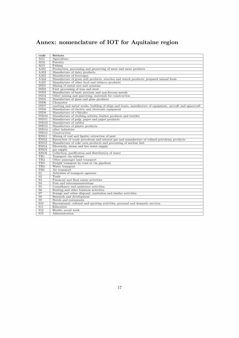
Annex: nomenclature of IOT for Aquitaine region

code SectorsAG1 AgricultureAG2 ForestryAG3 FishingAAI1 Production, processing and preserving of meat and meat productsAAI2 Manufacture of dairy productsAAI3 Manufacture of beveragesAAI4 Manufacture of grain mill products, starches and starch products, prepared animal feedsAAI5 Manufacture of other food and tobacco productsIND1 Mining of metal ores and uraniumIND2 First processing of iron and steelIND3 Manufacture of basic precious and non-ferrous metalsIND4 Other mining and quarrying, materials for constructionIND5 Manufacture of glass and glass productsIND6 ChemestryIND7 smelting and metal works, building of ships and boats, manufacture of equipment, aircraft and spacecraftIND8 Manufacture of electric and electronic equipmentIND9 Manufacture of v?hiculesIND10 Manufacture of clothing articles, leather products and textilesIND11 Manufacture of pulp, paper and paper productsIND12 Manufacture of rubberIND13 Manufacture of plastic productsIND14 other industriesIND15 ConstructionENG1 Mining of coal and lignite; extraction of peatENG2 Extraction of crude petroleum and natural gas and manufacture of refined petroleum productsENG3 Manufacture of coke oven products and processing of nuclear fuelENG4 Electricity, steam and hot water supplyENG5 gas supplyENG6 Collection, purification and distribution of waterTR1 Transport via railwaysTR2 Other passenger land transportTR3 Freight transport by road or via pipelinesTR4 Water transportTR5 Air transportS1 Activities of transport agenciesS2 TradeS3 Financial and Real estate activitiesS4 Post and telecommunicationsS5 Consultancy and assistance activitiesS6 Renting and other business activitiesS7 Sewage and refuse disposal, sanitation and similar activitiesS8 Research and developmentS9 Hotels and restaurantsS10 Recreational, cultural and sporting activities, personal and domestic servicesS11 EducationS12 Health, social workS13 Administration

17

ReferencesALMON C.(2000) Product-to-Product Tables via Product-Technology with No Negative Flows,Economic Systems Research, 12(1), pp. 27-43

AVONDS L. (2008) Evaluation d’un cadre entrées-sorties régional pour la Belgique, Workingpaper 18-08, Bureau fédéral du Plan

BERCK P. et HOFFMANN S. (2002) Assessing the Employment Impacts of Environmentaland Natural Resource Policy, Environmental and Resource Economics, 22 (1), pp.133-156

BOHLIN L., WIDELL L. (2006) Estimation of Commodity-by-Commodity Input-Output Ma-trices, Economic Systems Research, 18(2), pp. 205-215

BOOMSMA P., OOSTERHAVEN J. (1992) A double entry method for the construction ofbi-regional input-output tables, Journal of regional science, 32 (3), pp. 269-284.

BRAIBANT M (2006) Elaboration du tableau des entrées intermédiaires pour les années de base2000, INSEE, Paris

BRAND S. (1997) On the appropriate use of location quotients in generating regional input-output tables: a comment, Regional Studies, 31 (8), pp. 791-794

CHASE R.A., BOURQUE P.J., CONWAY R.S. (1993) The 1987 Washington state input-outputstudy, University of Washington

CORTINAS VAZQUEZ P., VICENTE VIRSEDA J.A. (2009) Tablas Input-Output de Castilla -La Mancha, III spanish input-output conference

COURBIS R. et POMMIER C.(1979) Construction d’un tableau d’échanges inter-industrielset inter-régionaux de l’économie française, Travaux du GAMA N◦4, Economica

DELFAUD P. (1982) Construction d’un modèle économique de prévision pour la région aquitaine,Research report for EPR Aquitaine, Laboratory of IERSO, University of Bordeaux I

DE MESNARD L. (2004a) On the Impossibility of Calculating the Product Technology in theSupply-Use Model, working paper, University of Bourgogne

DE MESNARD L. (2004b) Understanding the shortcomings of commodity-based technologyin input-output models: an economic-circuit approach, Journal of Regional Science, 44(1), pp.125-41.

DUARTE R., SANCHEZ-CHOLIZ J., BIELSA J. (2002) Water use in the Spanish economy:an input-output approach, Ecological Economics, 43(1), pp 71-85

EUROSTAT (2008) Eurostat Manual of Supply, Use and Input-Output Tables, Eurostat method-ologies and working papers

FLEGG A.T, WEBBER C.D., ELLIOTT M.V. (1995) On the appropriate use of location quo-

18

tients in generating regional input-output tables, regional studies, 31 (8), pp. 58-86

FLEGG A.T., WEBBER C.D. (1997) On the appropriate Use of Location Quotients in Gener-ating Regional Input-Output Tables: Reply, Regional Studies, 31 (8), pp. 795-805

FLEGG T., TOHMO T. (2008) Regional Input Output Models and the FLQ Formula: A CaseStudy of Finland, Economics Discussion Paper Series N◦08/08, School of Economics, Universityof the West of England

FRITZ O., KURZMANN R., ZAKARIAS G., STREICHER G. (2003) Constructing RegionalInput-Output Tables for Austria. Austrian Economic Quarterly, 8 (1), pp. 23-29.

HAWDON D., PEARSON P. (1995). Input-output simulations of energy, environment, economyinteractions in the UK, Energy Economics, 17 (1), pp. 73-86.

HUFBAUER G., (1970) The impact of national characteristics and technology on the com-modity composition of trade in Manufactured goods. In : R.Vernon, The technology factor ininternational trade, NBER Columbia press, pp.145-232.

ISARD W. (1951) Interregional and regional input-output analysis: A model of a space economy,The review of economics and statistics, 33(4), pp. 318-328

JANSEN K.P., RAA T.T. (1990) The choice of model in the construction of input-output coef-ficients matrices, International Economic Review, 31(1), pp. 213-227

JOUANDET-BERNADAT R. (1965) Le tableau interindustriel aquitain, Laboratory of IERSO,University of Bordeaux I

JOUANDET-BERNADAT R. (1967) Le tableau interindustriel régional, Revue économique, 18(3), pp. 447-479

KRONENBERG T. (2009) Construction of regional input-output tables using nonsurvey meth-ods: The role of cross-hauling, International Regional Science Review, 32 (1), pp. 40-64

LEONTIEF W., STROUT A. (1963) Multiregional input-output analysis. In : Barna T. ,structural independence and economic development, London: Macmillan, pp. 119-149. Reprintin Leontief W. (1986) Input-output economics, Oxford University Press, USA

LEONTIEF W. (1970) Environmental repercussions and the economic structure : An Input-Output Approach, Review of Economics and Statistics, 52 (3), pp.262-271

LEONTIEF W. (1986) Input-output economics, Oxford University Press, USA

LENZEN M. (2003) Environmentally important paths; linkages and key sectors in the Aus-tralian economy, structural change and economic dynamics, 14 (1), pp. 1-34.

LOVERIDGE S. (2004) A typology and assessment of multisector regional economic impactmodels, Regional studies, 38 (3), pp. 305-317.

19

MALINVAUD E. (1984) Aggregations problems in Input-output models. In : Barna T. : TheStructural Interdependence of the Economy, John Wiley, New York 1954, pp. 188-202

MATTAS K., PAGOULATOS A., DEBERTIN D. (1984) Builing IO models using non-surveytechniques, SRDC series 72, Southern rural development center, University of Kentuckey, De-partment of Agricultural economics, Mississippi State University, Mississippi.

MC GREGOR P.G.; SWALES J.K., TURNER K. (2008) The CO2 ’trade balance’ betweenScotland and the rest of the UK: Performing a multi-region environmental input-output analysiswith limited data, Ecological Economics, 66 (4), pp. 662-673

MILLER R.E., BLAIR P.D. (1985) Input-Output Analysis: Foundations and Extensions, Prenctice-Hall, Englewood Cliffs, NJ

MUNKSGAARD J., WIER M., LENZEN M, DAY C. (2005) Using input-output analysis tomeasure the environmental pressure of consumption at different spatial levels, Journal of indus-trial ecology, 9 (1-2), pp. 169-185.

OUSSET J. (1991) La comptabilité économique régionale en 1990, Les Cahiers de l’EconomieMéridionale, 14

PASINETTI L. (1977) Contributi alla teoria della produzione congiunta, Societá Editrice IlMulino, Bologna.

PROOPS J.L.R., FABER M., WAGENGHALS G., (1993) Reducing CO2 Emissions: A compar-ative Input-Output Study for Germany and the UK, Springer-Verlag, Heidelberg

RICHARDSON H.W. (1972) Input-output and regional economics, weidenfeld and Nicolson.

ROSE A., CASLER S. (1996) Input-Output structural decomposition analysis: a critical ap-praisal, Economic Systems Research, 8(1), pp. 33-62

ROUND J.I. (1978) An interregional input-output approach to the evaluation of nonsurvey meth-ods, Journal of Regional Science, 18(1), pp. 179-194.

SANCHEZ-CHOLIZ J., DUARTE. R. (2003a) Analysing pollution by way of vertically inte-grated coefficients with an application to the water sector in Aragon, Cambridge Journal ofEconomics, 27 (3), pp. 433-448.

SANCHEZ-CHOLIZ J., DUARTE R. (2003b) Production chains and linkage indicators, Eco-nomic Systems Research, 15 (4), pp. 481-494.

SANCHEZ-CHOLIZ J., DUARTE R. (2005) Water pollution in the Spanish economy : anal-ysis of sensitivity to production and environmental constraints, Ecological Economics, 53(3), pp.325-338

SCHAFFER W.A., CHU K. (1969) Nonsurvey techniques for construction regional interindustrymodels, papers in regional science, 23 (1), pp. 83-101

20

SHAFFER W.A., CHU K.(1969) Nonsurvey techniques for constructing regional interindustrytables, Papers and Proceedings of the Regional Science Association, 23 (83), pp. 105.

TEN RAA T., RUEDA-CANTUCHE J. (2007) A Generalized Expression for the Commod-ity and the Industry Technology Models in Input-Output Analysis, Economic Systems Research,19(1), pp. 99-104

TOHMO T. (2004) New Developments in the Use of Location Quotients to Estimate RegionalInput-Output Coefficients and Multipliers, Regional Studies, 38 (1), pp. 43-54

WEST G.R. (1995) Comparison of input-output, input-output econometric and computable gen-eral equilibrium impact, Economic Systems Research, 7(2), pp.209-228

WIEDMANN T. (2009) A review of recent multi-region input-output models used for consumption-based emission and resource accounting, Ecological economics, 69 (2), pp 211-222.

ZHANG Z.X., FOLMER H. (1998) Economic modelling approaches to cost estimates for thecontrol of carbon dioxide emissions, Energy economics, 20(1), pp.101-120.

21

Cahiers du GREThA Working papers of GREThA

GREThA UMR CNRS 5113

Université Montesquieu Bordeaux IV Avenue Léon Duguit

33608 PESSAC - FRANCE Tel : +33 (0)5.56.84.25.75 Fax : +33 (0)5.56.84.86.47

www.gretha.fr

Cahiers du GREThA (derniers numéros)

2010-11 : BROUILLAT Eric, LUNG Yannick, Spatial distribution of innovative activities and economic performances: A geographical-friendly model

2010-12 : DANTAS Monique, GASCHET Frédéric, POUYANNE Guillaume, Effets spatiaux du zonage sur les prix des logements sur le littoral : une approche hédoniste bayesienne

2010-13 : BLANCHETON Bertrand, SCARABELLO Jérôme, L'immigration italienne en France entre 1870 et 1914

2010-14 : BLANCHETON Bertrand, OPARA-OPIMBA Lambert, Foreign Direct Investment in Africa: What are the Key Factors of Attraction aside from Natural Resources?

2010-15 : ROUILLON Sébastien, Optimal decentralized management of a natural resource 2010-16 : CHANTELOT Sébastien, PERES Stéphanie, VIROL Stéphane, The geography of

French creative class: An exploratory spatial data analysis 2010-17 : FRIGANT Vincent, LAYAN Jean-Bernard, Une analyse comparée du commerce

international de composants automobiles entre la France et l’Allemagne : croiser un point de vue d’économie internationale et d’économie industrielle

2010-18 : BECUWE Stéphane, MABROUK Fatma, Migration internationale et commerce extérieur : quelles correspondances ?

2010-19 : BONIN Hubert, French investment banks and the earthquake of post-war shocks (1944-1946)

2010-20 : BONIN Hubert, Les banques savoyardes enracinées dans l’économie régionale (1860-1980s)

2011-01 : PEREAU Jean-Christophe, DOYEN Luc, LITTLE Rich, THEBAUD Olivier, The triple bottom line: Meeting ecological, economic and social goals with Individual Transferable Quotas

2011-02 : PEREAU Jean-Christophe, ROUILLON Sébastien, How to negotiate with Coase? 2011-03 : MARTIN Jean-Christophe, POINT Patrick, Economic impacts of development of road

transport for Aquitaine region for the period 2007-2013 subject to a climate plan 2011-04 : BERR Eric, Pouvoir et domination dans les politiques de développement 2011-05 : MARTIN Jean-Christophe, POINT Patrick, Construction of linkage indicators of

greenhouse gas emissions for Aquitaine region

La coordination scientifique des Cahiers du GREThA est assurée par Sylvie FERRARI et Vincent

FRIGANT. La mise en page est assurée par Dominique REBOLLO.