Construction of the proposal distribution for the particle

. . . . . .Introduction

. . .Ensemble transform Kalman filter

. . . . .Importance sampling

. . . . . .Reconstruction

. . . . . . . . . . .Experiment

.Summary

Construction of the proposal distribution for theparticle filter using the ensemble transform

Kalman filter

S. Nakano

The Institute of Statistical Mathematics

18 January 2013





. . . . . . . . . . .Experiment

.Summary

Particle filter..

The particle filter represents a probability density function (PDF) by aMonte Carlo approximation.The ensemble representing a posterior PDF is obtained by resampling aforecast ensemble.It is applicable even to the cases with non-linear or non-Gaussianobservations.However, it requires a huge number of particles to avoid the problemdue to ensemble degeneracy.

State x

State x

Forecast distribution

1: 1)( |k kp−

x y Likelihood

( | )k kp y x

Filtered distribution

1: 1: 1| ) ( | ) (( | )k k k k k kp p p−

∝x y y x x y





. . . . . . . . . . .Experiment

.Summary

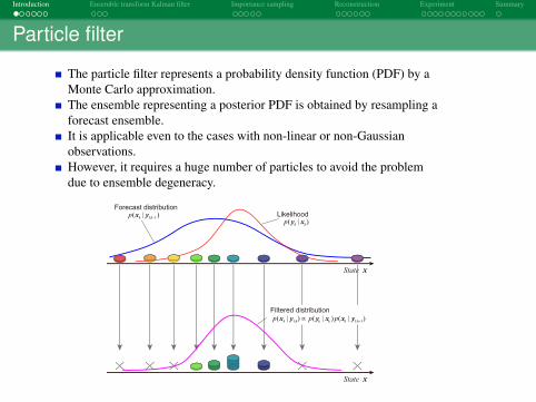
Particle filter..

The particle filter algorithm is based on the importance samplingmethod, which represents the posterior PDF by weighted sample.If we choose a good proposal distribution similar to the posterior PDF,the imbalance of weights among the particles can be reduced, andtherefore we could achieve high accuracy and high computationalefficiency.The prior (forecast) PDF is usually used as the proposal PDF. Thismakes the algorithm simple. But, a large discrepancy often existsbetween the prior PDF and the posterior PDF.

State x

State x

Proposal distribution

π(x)Weight function

( | ) ( )

( )

p y x p x

xπ

Posterior distribution

p(x|y)

State x

State x


p(x|y)


π(x)

Weight function( | ) ( )

( )

p y x p x

xπ





. . . . . . . . . . .Experiment

.Summary

Improvement of the proposal..Several studies have proposed a way to improve the proposal distribution.

Auxiliary particle filter (Pitt and Shephard, 1999).Nudge ensemble members toward the observation by considering thesystem noise (model error) (Chorin et al., 2010; van Leeuwen, 2010;2011).Weighted ensemble Kalman filter (Papadakis et al., 2010).





. . . . . . . . . . .Experiment

.Summary

Ensemble transform Kalman filter..

We use the ensemble transform Kalman filter (ETKF) (Bishop et al,2001) to obtain a proposal distribution for importance sampling, whichis similar to the weighted ensemble Kalman filter.In the ETKF, the first and second order moments of the PDF isrepresented by an ensemble.The ETKF algorithm is derived on the basis of the linear Gaussianobservation model.It therefore ignores non-Gaussian features of the PDF.The aim of using the importance sampling method is to representnon-Gaussian features of the PDF that is not considered by the ETKF.





. . . . . . . . . . .Experiment

.Summary

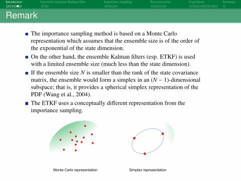
Remark..

The importance sampling method is based on a Monte Carlorepresentation which assumes that the ensemble size is of the order ofthe exponential of the state dimension.On the other hand, the ensemble Kalman filters (esp. ETKF) is usedwith a limited ensemble size (much less than the state dimension).If the ensemble size N is smaller than the rank of the state covariancematrix, the ensemble would form a simplex in an (N − 1)-dimensionalsubspace; that is, it provides a spherical simplex representation of thePDF (Wang et al., 2004).The ETKF uses a conceptually different representation from theimportance sampling.

Monte Carlo representation Simplex representation





. . . . . . . . . . .Experiment

.Summary

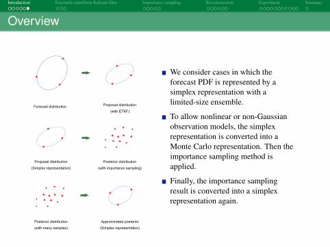
Overview


(with importance sampling)


(Simplex representation)


(with many samples)

Approximated posterior

(Simplex representation)

Forecast distribution Proposal distribution

(with ETKF)

We consider cases in which theforecast PDF is represented by asimplex representation with alimited-size ensemble.

To allow nonlinear or non-Gaussianobservation models, the simplexrepresentation is converted into aMonte Carlo representation. Then theimportance sampling method isapplied.

Finally, the importance samplingresult is converted into a simplexrepresentation again.





. . . . . . . . . . .Experiment

.Summary

Some definitions

Suppose that the forecast distribution is represented by an ensemble{x(1)

k|k−1, . . . , x(N)k|k−1}.

The mean of the forecast distribution is obtained as:

x̄k|k−1 =1N

N∑i=1

x(i)k|k−1.

We define a matrix Xk|k−1 and Yk|k−1 as

Xk|k−1 =1√

N

(δx(1)

k|k−1 · · · δx(N)k|k−1

), Yk|k−1 =

1√

N

(δy(1)

k|k−1 · · · δy(N)k|k−1

),

where δx(i)k|k−1 = x(i)

k|k−1 − xk|k−1 and δy(i)k|k−1 = Hk(x(i)

k|k−1) − Hk(xk|k−1), respectively,and we assumed the following observation model

yk = Hk(xk) + wk.

The covariance matrix of the forecast (predictive) distribution is written asVk|k−1 = Xk|k−1XT

k|k−1.





. . . . . . . . . . .Experiment

.Summary

Ensemble transform Kalman filter (ETKF) (Bishop et al.,2001)

The mean of the filtered distribution is obtained according to the Kalman filteralgorithm:

x†k|k = xk|k−1 + Kk(yk − Hkxk|k−1

)The square root of the covariance matrix is also calculated as X†k|k = Xk|k−1Tk,where the matrix Tk is designed to satisfy V†k|k = X†k|kX

†Tk|k and X†k|k1 = 0,

where 1 = (1 · · · 1)T . The latter condition is required to preserve the mean ofthe PDF (Wang et al., 2004; Livings et al., 2008).

Using the following eigen-value decomposition

Yk|k−1R−1k Yk|k−1 = UkΛkUT

k ,

the matrices Kk and Tk are obtained as follows:

Kk = Xk|k−1Uk(IN + Λk)−1UTk YT

k|k−1R−1k ,

Tk = Uk(IN + Λk)−12 UT

k ,

where Rk is the covariance matrix of the observation noise.





. . . . . . . . . . .Experiment

.Summary

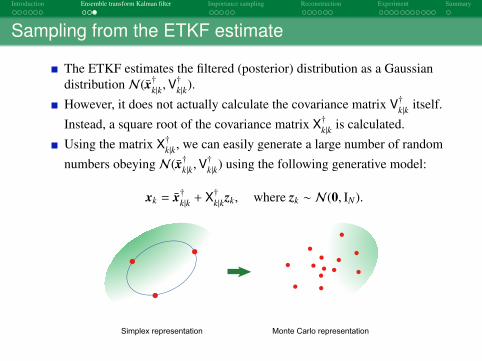
Sampling from the ETKF estimate..

The ETKF estimates the filtered (posterior) distribution as a Gaussiandistribution N(x̄†k|k,V

†k|k).

However, it does not actually calculate the covariance matrix V†k|k itself.Instead, a square root of the covariance matrix X†k|k is calculated.Using the matrix X†k|k, we can easily generate a large number of randomnumbers obeying N(x̄†k|k,V

†k|k) using the following generative model:

xk = x̄†k|k + X†k|kzk, where zk ∼ N(0, IN).

Monte Carlo representationSimplex representation





. . . . . . . . . . .Experiment

.Summary

Importance sampling

Since the posterior distribution p(xk |y1:k) is written as

p(xk |y1:k) =p(xk |y1:k)π(xk)

π(xk) =p(yk |xk)p(xk |y1:k−1)

p(yk |y1:k−1)π(xk)π(xk),

the posterior p(xk |y1:k) can be represented by the importance samplingusing the sample drawn from π(xk):

p(xk |y1:k) ≈M∑

j=1

p(yk |xπ(j)k )p(xπ(j)k |y1:k−1)

p(yk |y1:k−1)π(xπ(j)k )δ(xk − xπ(j)k ).

In the normal particle filter, the forecast p(xk |y1:k−1) is used as π(xk).On the other hand, we use the estimate of p(xk |y1:k) obtained by theETKF as the proposal π(xk).





. . . . . . . . . . .Experiment

.Summary

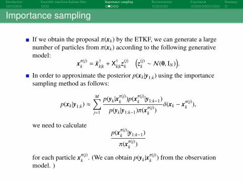
Importance sampling

If we obtain the proposal π(xk) by the ETKF, we can generate a largenumber of particles from π(xk) according to the following generativemodel:

xπ(j)k = x̄†k|k + X†k|kz(j)k

(z(j)

k ∼ N(0, IN)).

In order to approximate the posterior p(xk |y1:k) using the importancesampling method as follows:

p(xk |y1:k) ≈M∑

j=1


p(yk |y1:k−1)π(xπ(j)k )δ(xk − xπ(j)k ),

we need to calculatep(xπ(j)k |y1:k−1)

π(xπ(j)k )

for each particle xπ(j)k . (We can obtain p(yk |xπ(j)k ) from the observation

model. )





. . . . . . . . . . .Experiment

.Summary

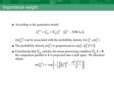
Importance weight

According to the generative model

xπ(j)k = x̄†k|k + X†k|kz(j)k

(z(j)

k ∼ N(0, IN)),

π(xπ,(j)k|k ) can be associated with the probability density for z(j)k , p(z(j)

k ).

The probability density p(z(j)k ) is proportional to exp

(−∥z(j)

k ∥2/2).

Considering that X†k|k satisfies the mean-preserving condition X†k|k1 = 0,the component parallel to 1 is projected onto a null space. We thereforeobtain

π(xπ,(j)k|k ) ∝ exp

−12

∥∥∥∥z(j)k

∥∥∥∥2 − (1Tz(j)k )2

N

.





. . . . . . . . . . .Experiment

.Summary

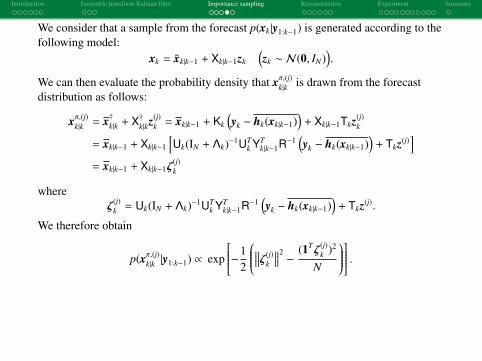
..We consider that a sample from the forecast p(xk |y1:k−1) is generated according to thefollowing model:

xk = x̄k|k−1 + Xk|k−1zk

(zk ∼ N(0, IN)

).

We can then evaluate the probability density that xπ,(j)k|k is drawn from the forecastdistribution as follows:

xπ,(j)k|k = x†k|k + X†k|kz(j)k = xk|k−1 + Kk

(yk − hk(xk|k−1)

)+ Xk|k−1Tkz(j)

k

= xk|k−1 + Xk|k−1

[Uk(IN + Λk)−1UT

k YTk|k−1R−1

(yk − hk(xk|k−1)

)+ Tkz(j)

]= xk|k−1 + Xk|k−1ζ

(j)k

whereζ(j)

k = Uk(IN + Λk)−1UTk YT

k|k−1R−1(yk − hk(xk|k−1)

)+ Tkz(j).

We therefore obtain

p(xπ,(j)k|k |y1:k−1) ∝ exp

−12

∥∥∥ζ(j)k

∥∥∥2 − (1Tζ(j)k )2

N

.





. . . . . . . . . . .Experiment

.Summary

As seen previously, the posterior distribution is approximated as

p(xk |y1:k) ≈M∑

j=1


p(yk |y1:k−1)π(xπ(j)k )δ(xk − xπ(j)k ).

If we generate the proposal sample according to the following model:

xπ,(j)k|k = x̄k|k−1 + Xk|k−1z(j)k

(z(j)

k ∼ N(0, IN)),

the weight for each particle can be given as follows:

β(j)k ∝

p(yk |xπ,(j)k|k ) exp

−12

∥∥∥ζ(j)k

∥∥∥2 − (1Tζ(j)k )2

N

exp

−12

∥∥∥z(j)k

∥∥∥2 − (1T z(j)k )2

N

.

We then obtain a new approximation of the posterior PDF:

p(xk |y1:k) ≈M∑

j=1

β(j)k δ(xk − xπ(j)k ).





. . . . . . . . . . .Experiment

.Summary

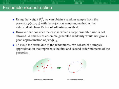
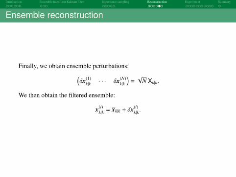
Ensemble reconstruction

Using the weight β(j)k , we can obtain a random sample from the

posterior p(xk |y1:k) with the rejection sampling method or theindependent chain Metropolis-Hastings method.However, we consider the case in which a large ensemble size is notallowed. A small-size ensemble generated randomly would not give agood approximation of p(xk |y1:k).To avoid the errors due to the randomness, we construct a simplexapproximation that represents the first and second order moments of theposterior.

Monte Carlo representation Simplex representation





. . . . . . . . . . .Experiment

.Summary

Moments on the z-space

If we calculate the mean and the covariance on the z-space:

z̄k =

M∑i=1

β(j)k z(j)

k , Vz,k|k =M∑

i=1

β(j)k (z(j)

k − z̄k)(z(j)k − z̄k)T ,

the mean and the covariance of the filtered distribution p(xk |y1:k) are given asfollows:

xk|k = x†k|k + X†k|k z̄k, Vk|k = Xk|kXTk|k = X†k|kVz,k|kX

†Tk|k

where x†k|k and X†k|k provide the estimate by the ETKF.

To avoid the bias of the ensemble mean, the new Xk|k should also satisfy

Xk|k1 = 0.





. . . . . . . . . . .Experiment

.Summary

We define the following matrix

A = IN −1N

1 · · · 1.... . .

...1 · · · 1

,which obviously satisfies

A1 = 0.

The covariance matrix Vk|k can then be written as follows:

Vk|k = X†k|kVz,k|kX†Tk|k

= X†k|kA Vz,k|kATX†Tk|k

because obviously X†k|k = X†k|kA.





. . . . . . . . . . .Experiment

.Summary

When we calculate the eigen-value decomposition of the matrix A Vz,k|kA as

A Vz,k|kA = Uz,kΓkUTz,k,

the matrix Uz,k contains an eigen-vector which is parallel to 1 andcorresponds to zero eigen-value. Therefore, if we define Xk|k as

Xk|k = X†k|kUz,kΓ12k UT

z,k,

it satisfies both of the necessary conditions:

Xk|kXTk|k = X†k|kVz,k|kX

†Tk|k,

Xk|k1 = 0.





. . . . . . . . . . .Experiment

.Summary

Ensemble reconstruction

Finally, we obtain ensemble perturbations:(δx(1)

k|k · · · δx(N)k|k

)=√

N Xk|k.

We then obtain the filtered ensemble:

x(i)k|k = xk|k + δx(i)

k|k.





. . . . . . . . . . .Experiment

.Summary

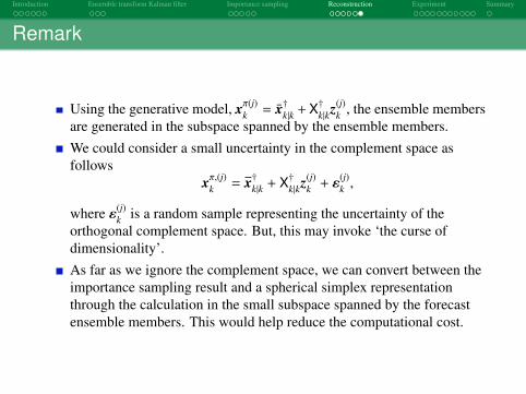
Remark

Using the generative model, xπ(j)k = x̄†k|k +X†k|kz(j)k , the ensemble members

are generated in the subspace spanned by the ensemble members.We could consider a small uncertainty in the complement space asfollows

xπ,(j)k = x†k|k + X†k|kz(j)k + ε

(j)k ,

where ε(j)k is a random sample representing the uncertainty of the

orthogonal complement space. But, this may invoke ‘the curse ofdimensionality’.As far as we ignore the complement space, we can convert between theimportance sampling result and a spherical simplex representationthrough the calculation in the small subspace spanned by the forecastensemble members. This would help reduce the computational cost.





. . . . . . . . . . .Experiment

.Summary

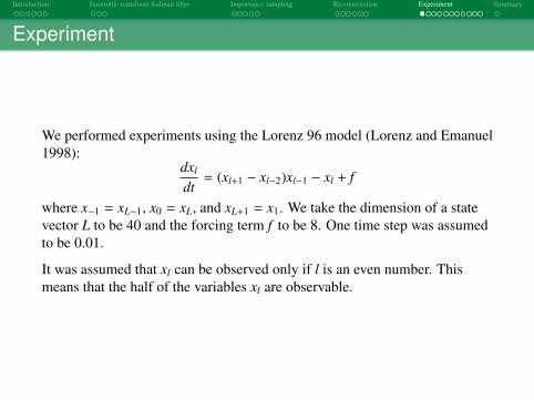
Experiment

We performed experiments using the Lorenz 96 model (Lorenz and Emanuel1998):

dxl

dt= (xl+1 − xl−2)xl−1 − xl + f

where x−1 = xL−1, x0 = xL, and xL+1 = x1. We take the dimension of a statevector L to be 40 and the forcing term f to be 8. One time step was assumedto be 0.01.

It was assumed that xl can be observed only if l is an even number. Thismeans that the half of the variables xl are observable.





. . . . . . . . . . .Experiment

.Summary

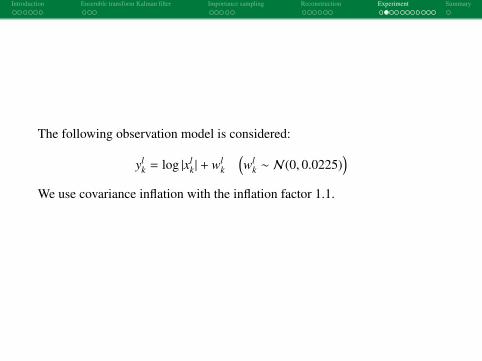
The following observation model is considered:

ylk = log |xl

k | + wlk

(wl

k ∼ N(0, 0.0225))

We use covariance inflation with the inflation factor 1.1.





. . . . . . . . . . .Experiment

.Summary

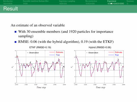
Result

An estimate of an observed variable

With 30 ensemble members (and 1920 particles for importancesampling)RMSE: 0.06 (with the hybrid algorithm), 0.19 (with the ETKF)

21000 21200 21400 21600 21800 22000

-10

-5

0

5

10

15

Time step

x2

21000 21200 21400 21600 21800 22000

-10

-5

0

5

10

15

Time step

x2

Estimate

True

Estimate

True

ETKF (RMSE=0.19) Hybrid (RMSE=0.06)

ObservationObservation





. . . . . . . . . . .Experiment

.Summary

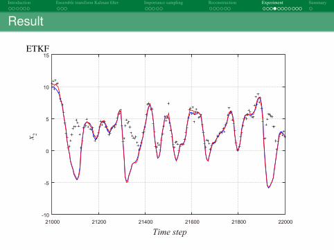
Result

ETKF

21000 21200 21400 21600 21800 22000

-10

-5

0

5

10

15

Time step

x2





. . . . . . . . . . .Experiment

.Summary

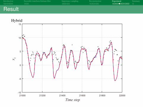
Result

Hybrid

21000 21200 21400 21600 21800 22000

-10

-5

0

5

10

15

Time step

x2





. . . . . . . . . . .Experiment

.Summary

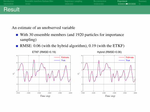
Result

An estimate of an unobserved variable


Time stepTime step


21000 21200 21400 21600 21800 22000

-10

-5

0

5

10

15

x1

21000 21200 21400 21600 21800 22000

-10

-5

0

5

10

15

x1

Estimate

True

Estimate

True





. . . . . . . . . . .Experiment

.Summary

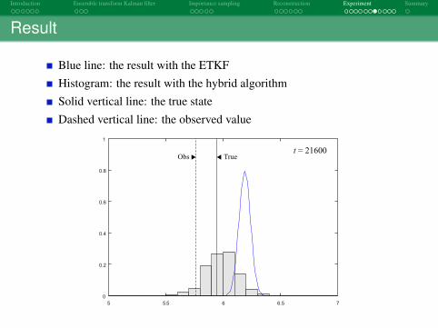
Result

Blue line: the result with the ETKFHistogram: the result with the hybrid algorithmSolid vertical line: the true stateDashed vertical line: the observed value

5 5.5 6 6.5 7

0

0.2

0.4

0.6

0.8

1

Obs Truet = 21600





. . . . . . . . . . .Experiment

.Summary

We also consider the following observation model:

ylk =∣∣∣xj

k + wjk

∣∣∣ (wjk ∼ N(0, 1)

),

The system noise is assumed as follows:

vlk ∼ N(0, 0.0625).





. . . . . . . . . . .Experiment

.Summary

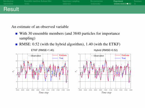
Result

An estimate of an observed variable


Time step

Estimate

True

Estimate

True


Observation

20000 20200 20400 20600 20800 21000 21200 21400 21600 21800 22000

-10

-5

0

5

10

15

x2

x2

Observation

Time step

20000 20200 20400 20600 20800 21000 21200 21400 21600 21800 22000

-10

-5

0

5

10

15





. . . . . . . . . . .Experiment

.Summary

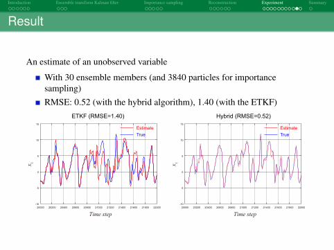
Result

An estimate of an unobserved variable


Time stepTime step


Estimate

True

Estimate

True

20000 20200 20400 20600 20800 21000 21200 21400 21600 21800 22000

-10

-5

0

5

10

15

x1

20000 20200 20400 20600 20800 21000 21200 21400 21600 21800 22000

-10

-5

0

5

10

15

x1





. . . . . . . . . . .Experiment

.Summary

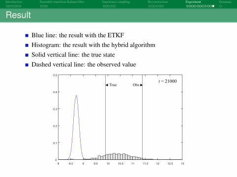
Result

Blue line: the result with the ETKFHistogram: the result with the hybrid algorithmSolid vertical line: the true stateDashed vertical line: the observed value

8 8.5 9 9.5 10 10.5 11 11.5 12 12.5 13

0

0.1

0.2

0.3

0.4

0.5

ObsTruet = 21000





. . . . . . . . . . .Experiment

.Summary

Summary

A good proposal distribution could improve the computationalefficiency of the particle filter.We propose a hybrid algorithm which use the ensemble transformKalman filter (ETKF) to obtain the proposal.While the importance sampling method used in the particle filterrequires abundant particles, the ETKF is based on a spherical simplexrepresentation which uses less particles than the state dimension. Wethen make the conversion between a simplex representation and aMonte Carlo representation.In our approach, this conversion is performed in the low-dimensionalsubspace spanned by the forecast ensemble members.Even though the uncertainty is considered only in the subspace, theproposed approach seems to well work in the cases with nonlinear,non-Gaussian observation models in which the application of ensembleKalman filters is not valid.

Documents

Construction of the proposal distribution for the particle