CE

UeT

DC

olle

ctio

n

Consumer Credit Scoring. An application using a Hungarian

dataset of consumer loans

by

Alexandru Constangioara

Submitted to

Central European University

Department of Economics

In partial fulfillment of the requirements for the degree of

Master of Arts in Economics

Supervisor: Prof. GÁBOR KÕRÖSI

Budapest, Hungary

2006

CE

UeT

DC

olle

ctio

n

i

Abstract

Following the significant development of consumer credit market after the 1980’s,

the risk management of consumer lending has become critical to protect the interests of

both lenders and consumers. Modeling default probabilities has received considerable

attention, both in theory and in practice.

After presenting the consumer credit market and introducing the main issues in

credit scoring, I use a Hungarian dataset of consumer loans to model the default

probabilities. The main research question refers to the comparative prediction accuracy of

Logit-Probit estimations, Discriminant analysis and Decisional tee. The results show that

they have similar prediction accuracy. The analysis of optimal cut-off threshold is

confined by the data available, considering only the losses from arrears. The predicted

default probabilities have been used to construct a credit score card.

CE

UeT

DC

olle

ctio

n

ii

Introduction .....................................................................................................1

Chapter 1 Consumer Credit Market..................................................................3

1.1Evolution.................................................................................................3

1.2 Activities and product offering ...............................................................4

1.3 Issues in the consumer credit market ......................................................5

1.4 Overview of the Hungarian consumer credit market ...............................6

Chapter 2 Credit scorecards .............................................................................8

2.1Types of Scorecards ................................................................................8

2.2 Statistical methods in Consumer Credit Scoring ...................................10

Chapter 3 Credit Risk Analysis using a Hungarian dataset .............................13

3.1 Variables and data ................................................................................14

3.2 Default probabilities and the efficiency of the models employed...........16

3.3 Maturity of the sample and Survival analysis........................................22

3.4 Cut-off threshold analysis.....................................................................25

3.5 Credit scores.........................................................................................27

Concluding remarks .......................................................................................29

References .....................................................................................................30

Appendices ....................................................................................................33

CE

UeT

DC

olle

ctio

n

1

Introduction

After 1980’s the Consumer credit market has known a significant increase both in

the value of outstanding amount and in the value of consumer credit relative to GDP and

households revenues (Siddiqui, 2006). Empirical studies show that the development of

market has led to over- indebtedness and consumer bankruptcy phenomena. Increasing

competition has fueled aggressive marketing techniques which have resulted in a deeper

penetration of the customers’ pool, and especially of low income customers, that usually

carry a higher debt burden, pay more interest and suffer more defaults. (Niu 2004) Under

these circumstances, the risk management of consumer lending has become critical to

protect the interest of both lenders and consumers.

There two major categories of risk in the market: systemic risk and credit risk.

Effective regulations and laws provide a safeguard for the industry from shocks that

might pose a systemic risk. Since the early work of Durant (1941) there has been

considerable interest in using statistical tools and risk management strategies to cope with

credit risk. Hand and Henley (1997) offer a summary of the statistical methods used in

the industry to predict credit risk.

The present paper offers an evaluation of the prediction accuracy of several

statistical methods used to analyze credit risk. In particular I use a Hungarian dataset to

compare the prediction accuracy of Logit and Probit Regressions to that of Discriminant

analysis and Decisional Tress.

Following the presentation of the main issue in the consumer credit market and

the introduction of credit scorecards, I will analyze a Hungarian dataset of loans for

CE

UeT

DC

olle

ctio

n

2

personal needs. The analysis will evaluate comparatively the prediction accuracy of

Logit-Probit estimations, Discriminant analysis and Decisional tree.

CE

UeT

DC

olle

ctio

n

3

Chapter 1 Consumer Credit Market

Consumer credit products cover general-purpose loans (personal loans), revolving

credit (with or without a plastic card), loans linked to specific purchase (such as point-of-

sale finance for cars and consumer durables) but not residential mortgage business

(Guardia, 2000). In general, consumer credit is not guaranteed whereas mortgage credit

uses property as collateral.

The consumer credit is difficult to measure for several reasons. Guardia (2000)

shows that in developing countries consumers arbitrage between the two, using the

cheaper mortgage credit for other purchases then property. This phenomenon has blurred

the distinction between consumer and mortgage credit. Another shortcoming is that most

countries report consumer credit outstanding (stock measure) which is different from

consumer credit flow (Guardia 2000).

1.1Evolution

Consumer credit outstandings amounted to around €900 BN at the end of 2003 in

EU 25. In comparison, the US market is larger, amounting at that time to $1.8 TN or

around $6000 per capita. In Europe data show strong concentration. The United

Kingdom, Germany and France are Europe’s three biggest consumer credit markets

(Mercer Oliver 2005 Report). The market penetration is better measured by consumer

outstanding relative to GDP or relative to household income. Over the period 1996-2000,

Weill (2004) argues that there was a quasi-general increase in both ratios for EU25

countries. Same author summarizes the factors which contribute to the differences in the

development of consumer credit across EU25. Thus he points to demand side factors

CE

UeT

DC

olle

ctio

n

4

(development of financial markets, regulatory framework and judicial systems) and to

supply side effects (cultural factors which might drive the attitude towards consumer

credit). Mercer Oliver Wyman 2005 Report (Mercer Report) also shows that regulatory

factors as responsible for the relatively low development of the market in countries like

Switzerland for example, which has similar market penetration as Hungary, Poland or

Czech Republic (~2% of GDP).

Both Mercer Report and the White Paper point to the differences between EU 15

countries and the new entrants. Although new entrants have historically little consumer

credit and les purchasing power, their consumer credit markets have high growth

potential.

1.2 Activities and product offering

There are three main activities within consumer credit financing. Vehicle

financing is one important activity within consumer credit, representing between one-fifth

and two-thirds of consumer credit outstandings. Point-of-sale financing, the second

important segment of consumer credit market offers credit facilities at a point of sale. It

covers long term goods and also services as travel, health, entertainment, accounting for

one fifth of the market by the same report. Direct financing segment has two main

characteristic: the customer establish a direct relationship with the financing entity and

the loan is not linked to a specific purchase. This segment is more developed in Germany

and Netherlands and less developed in Italy, France and Spain (Mercer Report).

CE

UeT

DC

olle

ctio

n

5

1.3 Issues in the consumer credit market

There are two main tendencies in the market, as anticipated by basic business

logic. One of them is specialization. Some players have specialized in different value-

adding services, such as risk management, call centers, IT platforms or business

prospecting. The other tendency is concentration in order to achieve economies of scale.

Going pan-European is a trend that already can be discerned by looking at the number of

players that are operating across Europe.

A major concern regarding the consumer credit market is the increasing over-

indebtedness. Household indebtedness has received much attention in recent empirical

studies The White paper on the reform of UK consumer credit market (White paper) uses

three criteria to define over-indebtedness: 25% of the household income is spent on

repaying consumer credits, 50% is spent on consumer credit and mortgages and the

household has four or more credit commitments. Either one of them defines over-

indebtedness.

Empirical studies show an increase in the households’ indebtedness. For the

debtors most relevant is the extent of the impact of over-indebtedness on households’

ability to service their debt. Rinaldi and Sanchis (2006) document the households’ ability

to service debt in spite of the development of new financial products and of deeper

penetration of the market. However Bridges and Disney (2003), using the Survey of Low

Income Families in UK have found evidence of increasing debt and arrears among the

low income families in UK.

To address the over-indebtedness phenomenon regulation is essential. Thus

regulation ensures a fair, safe and competitive market environment serving al the

CE

UeT

DC

olle

ctio

n

6

stakeholders. Its regulatory environment is rapidly catching with the US both at national

at EU level. In several central and northern European countries judicial debt adjustment

lows are already in place where as the Treaty of Amsterdam has already addressed the

problem of cooperation in this field. However aspects such as consumer protection, debt

collection and debt enforcement still have to be addressed. However both Merger Report

and the White Paper agree that reform of the European Consumer Credit Market is still

needed to promote “an open and fair consumer credit market where consumers can make

fully informed decisions and businesses can compete aggressively on a fair and even

basis” (White Paper).

1.4 Overview of the Hungarian consumer credit market

At the beginning of 1990’s the newly created commercial banks had inherited

portfolios of bad loans. Strict regulation and adopting adequate risk management

strategies helped them to survive the difficulties of the transition period.

A report from National Bank of Hungary (2005) shows the main evolutions in the

Hungarian consumer credit market after 1999. Figure 1.1 shows that consumer credit

market has developed from 5% of GDP in 1999 to 20% in 2005.

CE

UeT

DC

olle

ctio

n

7

Figure 1.1 Hungarian Consumer Credit Market

0

5

10

15

20

25

Jun.

99

Dec

. 99

Jun.

00

Dec

. 00

Jun.

01

Dec

. 01

Jun.

02

Dec

. 02

Jun.

03

Dec

. 03

Jun.

04

Dec

. 04

Jun.

05

%

44

50

56

62

68

74%

Housing loans / GDP (left hand scale) Consumer loans / GDP (left hand scale)Share of consumer loans (right hand scale)

Source: Report on Financial Stability, National Bank of Hungary, 2005

The same report of National Bank of Hungary shows that consumers’

indebtedness has declined after 2000. The main reason is the unemployment. However,

the prospects for the next period are encouraging as, according to the same report, the

wages are expected to grow.

CE

UeT

DC

olle

ctio

n

8

Chapter 2 Credit scorecards

Credit scorecards are the main tool used in assessing the credit risk in consumer

credit market.

2.1Types of Scorecards

There are three types of credit scorecards Subjective scoring is based mainly on

intuition. However Schreiner (2003) shows that it uses qualitative judgment and even

quantitative guidelines to evaluate the creditworthiness of applicants. The main advantage

of subjective scoring is convenience; in their case there is no need to build a credit history

database. Of course this comes at the expense of inadequate predictive accuracy and

subjective judgment.

Expert systems provide the second category of scorecards. They are derived from

the experience of managers and loan officers. While subjective scorecards use mainly

implicit judgment, expert systems are based on explicit rules, statistics or mathematics.

The simplest expert system is a Decisional Tree those splits come from experience and

not from statistical analysis of the data. However statistical analysis can be used to

control the growth of the Tree.

The third type of scoring uses statistical analysis to predict the credit risk

explicitly as a probability. Once the risk is determined, the credit committee selects

applicants using existing policies1. Most used is the four-class scoring policy. It consists

1 The process starts when an application is submitted. The application is first screened against

basic policy rules, such as the minimum one year tenure. If this criterion is met, the loan officer will

CE

UeT

DC

olle

ctio

n

9

in identifying four classes of risks: ”super-good” class, “normal” risk class, “border-line”,

and “super-bad” risk class (Schreiner, 2003).

Credit scores indicate the trade-off between the risks and the penetration of the

market, measured by depth, breadth and length2. By making the process automatic (i.e.

rejecting automatically super-bad applicants), scoring can save time which can be used to

increase the market penetration.. The credit officer will have more time to dedicate to low

risk applications which will result in reaching more customers and more segments. Since

the risk is better evaluated the scoring will the companies’ efficiency. Schreiner (2003),

analyzing the benefits of scoring concludes that it improves the efficiency of lenders. But

he also identifies fives type of costs associated with scoring: data accumulation, setup,

operational, policy-induced3 and process costs. They are related to building and

maintaining a credit history database needed to assess the credit risk. Most micro lenders

simply do not have the data needed for this purpose4. Then scoring takes time to build

analyze the file. After that the data will be introduced into the informational system and a credit score will

be computed. The credit committee will use the credit score to screen the applicants (Schreiner, 2003).

2 Depth shows the targeted segments; Breadth shows the penetration of each segment; Length

measured the profits obtained.

3 Policy induced costs refers to rewards to super-good applicants and to the fact that some of the

rejected applications would have been good.

4 Building own databases with credit history of the applicants is essential in Behavioral Scoring.

However, Credit Bureaus play the most important role in assessing the underwriting risk. In US and a few

European countries, credit bureaus or credit risk management agencies offer comprehensive credit history

information synthesized in a credit score, used afterwards together with other information regarding the

applicant to assess the applicants’ credit worthiness.

CE

UeT

DC

olle

ctio

n

10

scorecards, to implement them and not ultimately to accommodate the personnel with

them, due to the novelty of statistical scorecards (Schreiner, 2003).

One important aspect underlined by existing literature is the fact that different

types of scoring should complement each other. Although the net benefits of statistical

scoring might be considerable, not all the characteristics can be quantifies. All the

literature on credit risk management shows that qualitative characteristics of the

borrower, especially its willingness to pay of prime importance in assessing his credit

risk. This might be one of the reasons why existing studies, although point out to the

increasing indebtedness of consumers and its potential impact on their ability to service

their loans (Rinaldi and Sanchis, 2006), find similarities between low and high income

borrowers in terms of the partial effect of the variable associated with the quality of the

credit on the dependent variable (Sexton, 1977)5.

2.2 Statistical methods in Consumer Credit Scoring

A summary of the statistical methods for assessing credit risk is offered by Hand

and Henley (1997). Statistical scoring uses predictor variables to yields probabilities of

default or to predict the repayment behavior of borrowers. Schreiner (2003) argues that

Regression estimations, Discriminant analysis and Decisional trees are the most prevalent

statistical methods that are used in assessing credit risk. However more sophisticated

methods such as nonparametric smoothening, mathematical programming, Markov

chains, recursive partitioning, genetic algorithms or neural networks are also available.

5 The author fails to find statistically significant coefficient differences between low income and

high income families;

CE

UeT

DC

olle

ctio

n

11

2.2.1 Binary Logit and Probit models

Logistic regression considers the existence of an unobserved response variable Y*

which can be thought of as the "propensity towards" the event of interest, i.e. default on a

loan.

The variable is defined by Y*= b’Xi +Ui; what can be observed is a dummy variable, a

realization of a binomial process defined by Y=

From these relations we can derive the probability of the event of interest.

iprob( 1) prob(b' 0) 1 ( ' )i i iY X U F b X (2.1)

The Logit model assumes a logistic distribution of the error term while the Probit model

assumes standard normal distribution of ui. Thereby the probability of interest is:

For Logit model: exp( ' )Pr( 1| )1 exp( ' )

ii i

i

b XY Xb X

(2.2)

For Probit model:2'

Pr( 1 | ) 2 exp( )2

b iX ii i

zY X dz (2.3)

The parameters are estimated by Maximum Likelihood which maximizes the Probit

likelihood function for Probit model and Logit likelihood function for Logit model.

Logit and Probit estimation of credit risk have received a lot of attention in the

credit risk literature. On theoretical grounds they are considered a more appropriate

statistical tool for estimating probabilities than linear probability model. As Schreiner

(2003) shows, empirical results tend to agree with theoretical predictions. Nevertheless,

Hand and Henley (1997) argue that if a large proportion of the applicants have estimated

default probabilities between 0.2 and 0.8 the logistic and normal curve are well

approximated by a straight line and Linear Probability Model can give similar results.

1 if Y*i >0

0 if Y*i<0

CE

UeT

DC

olle

ctio

n

12

2.2.2 Discriminant Analysis

Discriminant analysis generates a Discriminant function that is used to predict

group membership based on observed characteristics of observations. The Discriminant

function is thereby:

Di b0 b1 xi1b2 xi2 bpxi p

(2.4)

The reason for this is not necessary its prediction accuracy but its strong

assumptions, and above all the assumption that exogenous variables are normally

distributed. Hand and Henley (1997) present an analytical overview of the main criticism

and advantages of Discriminant Analysis in economics.

2.2.3 Decisional Trees

The Decisional Tree classifies cases into groups or predicts values of a dependent

(target) variable based on values of independent variables. Statistical packages provide

possibility to control the growth of the tree i.e. the number of levels beneath the root node

by setting a minimum number of cases for each node for example. Also different methods

provide automatically a maximum tree depth. As in the case of other methods, several

statistics are available to validate the model i.e. to determine how well the model fits the

data. Decisional Tree it is the simplest statistical method to model credit risk, as

considered the existing credit risk literature. However it can be efficient, as subsequent

analysis will show.

CE

UeT

DC

olle

ctio

n

13

Chapter 3 Credit Risk Analysis using a Hungarian dataset

To model default probabilities one must define default. In the credit risk industry

default is defined using either the “ever bad” definition or the “current bad” definition

(Siddiqi, 2006). For the present analysis I have considered as defaulted an account that

ever accumulated arrears, regardless of their size and tenure. Basel 2 accord recommends

a 90 days delinquent definition (Siddiqi, 2006). However I have chosen the “ever

delinquent” definition regardless of the size of arrears because of the characteristics of the

dataset (small number of delinquent cases, short observation period).

There are several issues that might bias the analysis of credit risk. A first issue is

that the monitoring period of arrears is short, which raises the question regarding the

maturity of the accounts. Immature accounts are considered those which do not have time

to “go bad”6. In practice behavioral scorecards need to rely on at least a two years

observation period (Siddiqui, 2006). On the other hand, using data on existing accounts to

predict default probabilities is problematic because of selection bias issue - the default

accounts are not selected randomly from the sample of applicants. Siddiqui (2006)

stresses that the developing sample must include an equal number of defaults, non-default

and rejected cases. An adequate solution for this problem would be to estimate a system

of equations, one for default probability and the other for the probability that one receives

a loan. Another issue that might compromise the results is the population drift. This refers

to changes in time in the distribution of population. This issue is particularly relevant for

6 Definition of “bad” will be addressed later in the analysis.

CE

UeT

DC

olle

ctio

n

14

transition economies, as Natasa Sarlija ET all (2007) have found in a study using

Croatian data.

3.1 Variables and data

I have used an anonymous Hungarian dataset of 5060 observation of existing

accounts of loans for personal needs. The list of the variables used in the analysis is

presented in Appendix A, Figure A1.

There are three groups of variables. A first group consists of demographic

characteristics. A second group of variable refers to the financial situation of the

borrower and the third refers to the loan and re-payment history. The old scoring date

variable has been used to determine the tenure of the accounts. In the analysis I have

constructed several banded variables. To determine the optimum segmentation I have

used a tree analysis, with default variable as a dependent variable. An example is given in

Figure 3.1.

CE

UeT

DC

olle

ctio

n

15

Figure 3.1 Aggregation for AGE using Tree analysis

Node 0

Category % n

95.4 48280.0004.6 2311.000

Total 100 .0 5059

age[years]Adj. P-value=0.000, Chi-square=23.

556, df=2

arrears ever

Node 1

Category % n

94.4 28140.0005.6 1681.000

Total 58.9 2982

<= 39

Node 2

Category % n

96.4 15400.0003.6 571.000

Total 31.6 1597

(39, 54]

Node 3

Category % n

98.8 4740.0001.2 61.000

Total 9.5 480

> 54

0.0001.000

We see that for AGE variable we can distinguish three groups: less than 39 years,

between 39-54 years and above 54 years. The default probability for each branch is given

in the Tree Graph (Figure 3.1). The statistical significance of the splitting nodes is under

5%. The Figure 3.1 also reveals that younger people have higher default probabilities.

The data description is presented in Table A2, Appendix A. The examination of

variables, corroborated with the Test of equality of group means (Table 3.1) offers

interesting information. Most interesting is the fact that default accounts have higher net

income (INCOME) than non-default cases (although we cannot reject the hypothesis of

equal income means for the two groups). Moreover, most default cases come from

Budapest residents. We also cannot reject the hypothesis of equal means for HUNG

variable. The other variables offer no surprises: default cases are associates with less

educated, single, younger persons, with less tenure with current employer.

CE

UeT

DC

olle

ctio

n

16

Table 3.1 Tests of Equality of Group Means

Variables Sig.

INCOME .19MEMBERS .00MARITAL .00EDU .00INV_P .01LIFE_I .00C_ACC .00HUNG .79REGION .00TENURE .00AGE .00INC_BAND .00AGE_BAND .00tenure_band .00

Unfortunately the dataset does not offer information that would be useful for

analyzing the borrower’s portfolio of accounts. There is no information about the granted

amount, monthly installments, early redemptions or costs associated with accounts (other

than those from arrears). Such information would be necessary to adequately estimate the

costs from defaults and the optimum threshold level of risk.

3.2 Default probabilities and the efficiency of the models employed

To model default probabilities I have used Logistic regression, Discriminant

analysis and Decisional Trees. For each statistical method I have used two models

(A and B).

3.2.1 Logit and Probit estimations

The estimated coefficients and their significance levels for Regression estimations

are presented in the Table 3.2.

CE

UeT

DC

olle

ctio

n

17

Table 3.2 Regressions’ estimates

Logit ProbitB A B AVariables

p-value p-value p-value p-valueMARITAL -0.35 0.03 -0.40 0.01 -0.17 0.02 -0.17 0.02

MEMBERS -0.29 0.00 -0.30 0.00 -0.15 0.00 -0.16 0.00EDU -0.47 0.00 -0.44 0.00 -0.24 0.00 -0.23 0.00

C_ACC -0.57 0.00 -0.60 0.00 -0.29 0.00 -0.30 0.00INV_P -0.28 0.07 -0.25 0.13 -0.14 0.07 -0.12 0.11LIFE_I -0.24 0.14 -0.27 0.09 -0.09 0.11 -0.12 0.10

REGION 0.46 0.01 0.61 0.00 0.24 0.01 0.29 0.00AGE -0.02 0.00 -0.01 0.00

AGE_BAND -0.31 0.01 -0.16 0.01TENURE_BAND -0.50 0.00 -0.26 0.00

INC_BAND 0.72 0.00 0.31 0.00INC 0.00 0.08 0.00 0.13

* Huber/White standard errors & covariance have been used

LIFE_I is not significant at 10% level and INC variable is not significant at low

levels (below 5%). Variables that were found to be significant are broadly the same as

those reported in previous empirical literature7. The coefficients can’t be interpreted

directly in Logit and Probit estimations. However we can infer valuable information from

the sign of the coefficients. For both Logit and Probit models, Income variables (INC,

INC_BAND) have a positive estimated coefficient. For INC the coefficient is close to

zero but for INC_BAND is the largest for all coefficients in absolute value. Thereby the

probability of default increases with the income of the borrower. This is quite counter –

intuitive. However it accords with previous empirical findings. Jacobson and Roszbach

7 Natasa Sarlija et all (2007) argues that for consumer credit scoring the variable found to be

significant in empirical studies are: time at present address, marital status, postcode, telephone, applicant's

annual income, owing a credit card, type of bank account, age, type of occupation, purpose of loan, time

with bank, time with employer, credit bureau rating, monthly debt as a proportion of monthly income, time

at current job and number of dependents.

CE

UeT

DC

olle

ctio

n

18

(1998) consider that the positive partial effect of income on default probability might be

attributable to other personal characteristics associated with higher income. Mark

Schreiner (2003) uses the same argument to emphasize the role of credit officer in

judging the credit worthiness of the applicant. The results also show a positive

coefficient on REGION. Observations from Budapest residents have a higher default

probability. Same explanation can be applied here, considering that wages tend to be

higher in Budapest. The other coefficients have the expected sign.

A first clue about the models’ ability to fit the data is offered by Hosmer and

Lemeshow (H-L) test, reported in Table 3.3. H-L Test’ results show that all the models

fit the data adequately. Based on a 5% cut-off probability both Probit and Logit models

predict correctly ~95% of the observations. The models do very well in predicting non-

default cases but fail for default cases. This is not surprising considering the sample

proportion of the default cases (~4%). Additional information about the models’

prediction accuracy is given by the gains from the comparison of models’ predictions

with the restricted models, presented in Table 3.3.

Table 3.3 Prediction accuracy of regression estimations

Logistic Regressions Probit RegressionB A B APrediction accuracy

Correct%

Gain%

Correct%

Gain%

Correct%

Gain%

Correct%

Gain%

0 95.51 3.14 95.48 2.30 95.48 0.70 95.31 -0.171 9.96 4.54 8.52 2.86 7.98 4.84 7.26 3.23

Total 91.55 3.84 93.20 2.58 91.45 2.77 91.38 1.53H-L test 0.40 0.82 0.28 0.30

The gain resulted from comparison with the restricted model shows that Logit

models do better than Probit models. Also the prediction accuracy improves when the

constructed (banded) variables are used.

CE

UeT

DC

olle

ctio

n

19

3.2.2 Discriminant analysis

Given a set of independent variables, Discriminant analysis attempts to find linear

combinations of those variables that best separate the groups. These combinations are

called Discriminant functions. As I have shown previously, the weakness of Discriminant

analysis relies in its strong assumption, particularly the one about the normal distribution

of the predictors.

For model specification I have used forward stepwise selection, available in

SPSS. The coefficients of the classification function are given in the table below.

Table 3.4 Coefficients of the Discriminant Function

Discriminant model B Discriminant model AVariables

default=0 default=1 default=0 default=1MEMBERS 2.98 2.79 2.82 2.63MARITAL -0.95 -1.40 0.07 -0.46INV_P 3.00 2.66 4.19 3.83C_ACC 2.71 1.88 3.48 2.67INC-BAND 5.39 6.08TENURE_BAND 3.03 2.56TENURE 0.05 0.01REGION 1.21 1.97GENDER 2.99 3.35C -14.76 -16.16 -8.42 -10.07

The coefficients are used to obtain statistically different scores for the two classes

of accounts. There are several statistics reported by SPSS which assess the contribution

of each variable to the model. For both models, the variables in the analysis have high

tolerance (~0.98). Tolerance is the proportion of a variable’s variance not accounted for

by other independent variables. High Tolerance shows a strong contribution of the

selected variable to the model. SPSS also reports the statistical significance of the

CE

UeT

DC

olle

ctio

n

20

variables that are left in the model at each step of the forward stepwise procedure. All the

variables in the two models are highly significant (p<5%).

In addition for checking the contribution of individual predictors to the

Discriminant model, the Discriminant Analysis provides the Eigen values and Wilks'

lambda tables for seeing how well the Discriminant model as a whole fits the data. Wilks'

lambda is a measure of how well each function separates cases into groups. It is equal to

the proportion of the total variance in the Discriminant scores not explained by

differences among the groups. A high Wilks’ Lambda (~0.97 in both cases) is evidence

that the Discriminant function is not efficient in discriminating between groups.

However, the associated Chi-square which tests the hypothesis that the means of the

function are equal across groups is highly significant for both models (p=0.00).

My analysis shows that the prediction accuracy of the Discriminant analysis is

comparable to that of previous regressions. Discriminant models have been constructed

using all the observations in the dataset. A cross validation procedure has been used to

validate the results. For both models, the classification results show 95.4 % prediction

accuracy, based on a 0.5 cut-off value. Once again, the models do very well in predicting

non-default cases but fail for default-cases.

3.2.3 Tree analysis

The Tree depth is three by default for CHAID method. The tree growth is

controlled by different requirements such as minimum number of cases in parent node

(100), minimum number of cases in child node (50). By model construction, a split is

generated only if its statistical significance is under 5%. The Tree diagrams are presented

in APPENDIX B, Figure B1 and B2. The overall prediction accuracy of the models is

CE

UeT

DC

olle

ctio

n

21

~95%. Once again, both models fail to correctly identify the default cases. Cross-

validation procedure has been used to validate the models. Thus I have found evidence

that Tree analysis, although simply can be as accurate as Regressions or Discriminant

analysis. In addition Tree analysis offers other valuable information for credit risk

assessment. Siddiqui (2006) argues that Tree analysis identify whether it is necessary to

use different scorecards for different groups of the population. For example, based on the

Tree model A (Figure B2), the policy makers might decide to use separate score cards for

married and unmarried applicants. If this is the case, each scorecard might use different

variables to asses the default risk. Nevertheless, the statistical arguments -although

necessary- are not enough for segmentation decisions because of the costs implied.

3.2.4 Efficiency of the models

The efficiency of the models is considered from the perspective of their predictive

accuracy. The classification results show similar results. Further analysis will use the

ROC curve, a visual index of the accuracy of the models. Two ROC curves are presented

in ANNEX C, Figures C1-C4.

CE

UeT

DC

olle

ctio

n

22

Table 3.5 Main results of ROC analysis

Area under the Curve Area p-values

Logit analysis B 0.748 0.00

Probit analysis B 0.747 0.00

Discriminant analysis B 0.732 0.00

Tree analysis A 0.728 0.00

Tree analysis B 0.727 0.00

Logit analysis A 0.698 0.00

Probit analysis A 0.697 0.00

Discriminant analysis A 0.692 0.00

Null hypothesis: true area = 0.5* 3 decimal points are presented to allow differentiating between the models’ accuracy

Table 3.5 shows the prediction accuracy of the models according to ROC

analysis. Once again the analysis shows similar results. There are however a few

interesting findings. First of all, the ROC analysis reveals that B-Models tend to do better

than A-models. A second finding is that tree analysis has unexpectedly good prediction

accuracy. For Regression estimations the results of the ROC curve are mixed, depending

on the specification. While B-models have the best accuracy among all models, A-models

are outperformed by B-specification of both Discriminant analysis and Decisional Trees.

3.3 Maturity of the sample and Survival analysis

The reliability of the predicted probabilities depends, among other considerations,

on the maturity of the accounts. The accounts were opened from May to August 2005.

Arrears are registered only in three observation periods: November 2005, January 2006

CE

UeT

DC

olle

ctio

n

23

and February 2006. The short observation period of the arrears raises the question about

their maturity.

Most accounts in the dataset have accumulated arrears after four, five or six

months - 66% of all the accounts who ever accumulate arrears are in this situation. After

eight months, the number of accounts who accumulate debt drops significantly (there is

only one account in this situation). However the issue of the maturity of the accounts is

still unanswered because there are only 314 accounts older than 8 months in the sample

(6.2% of all the accounts). Moreover, within a given tenure period, the proportion of

accounts with arrears increases with tenure; for accounts with 9 months tenure the ratio is

0.10%, more than twice the overall sample’s ratio (0.04%). This indicates the possibility

that the sample is immature. However further investigation is needed to in this issue.

I have conducted a Cox Regression analysis of the survival of accounts, using a

forward stepwise method for model specification. Hazard rate is the probability of

instantaneous occurrence of an event conditional on the fact that the event has not

occurred until that moment. Thus hazard rate is defined by the relations

( | )lim pr t T t h T t

h o

(3.1)

( | ) exp( ' ) ( )t x x b t (3.2)

( )t is the baseline hazard. The coefficients of the regression are statistically significant

(p<5%). Also the change in -2 Log Likelihood for each step of the stepwise forward

selection used to construct the model is also statistically significant (p=0.00).

CE

UeT

DC

olle

ctio

n

24

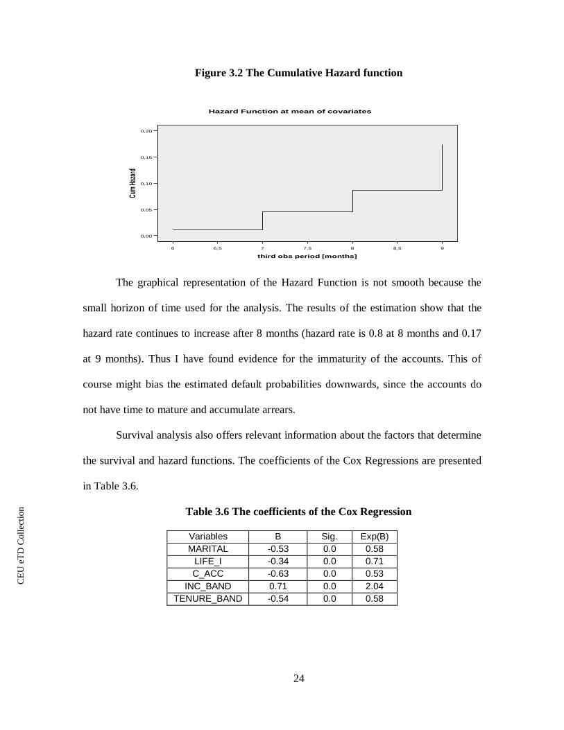
Figure 3.2 The Cumulative Hazard function

98,587,576,56

third obs period [months]

0,20

0,15

0,10

0,05

0,00

Cum

Hazar

d

Hazard Function at mean of covariates

The graphical representation of the Hazard Function is not smooth because the

small horizon of time used for the analysis. The results of the estimation show that the

hazard rate continues to increase after 8 months (hazard rate is 0.8 at 8 months and 0.17

at 9 months). Thus I have found evidence for the immaturity of the accounts. This of

course might bias the estimated default probabilities downwards, since the accounts do

not have time to mature and accumulate arrears.

Survival analysis also offers relevant information about the factors that determine

the survival and hazard functions. The coefficients of the Cox Regressions are presented

in Table 3.6.

Table 3.6 The coefficients of the Cox Regression

Variables B Sig. Exp(B)MARITAL -0.53 0.0 0.58

LIFE_I -0.34 0.0 0.71C_ACC -0.63 0.0 0.53

INC_BAND 0.71 0.0 2.04TENURE_BAND -0.54 0.0 0.58

CE

UeT

DC

olle

ctio

n

25

All the coefficients are statistically significant (p=0.00). As in Logit and Probit

estimations, For INC_BAND the hazard increases with the income. This is once again

counter-intuitive but in accordance with previous empirical findings (Jacobson and

Roszbach, 1998). Same explanation is plausible – there might be personal characteristics

of the borrower related with higher income that affect the probability to accumulate

arrears. The B-coefficients are not directly interpretable. SPSS also reports the Exp (B)

values. They represent the predicted change in the hazard for one unit increase in the

predictor.

3.4 Cut-off threshold analysis

The models used to estimate the default probabilities have failed to correctly

identify the default cases at a 0.5% cut-off value. Additional research is needed to

determine the most appropriate threshold. One possibility is to choose the threshold in

order to minimize the costs incurred. Unfortunately the dataset don’t offer information

about the granted amount, monthly installments, early redemptions or other costs

associated with accounts (other than those from arrears). Such information would be

necessary to adequately estimate the costs from defaults and the optimum threshold level

of risk. Thereby in the subsequent analysis I will consider only the costs associated with

arrears.

Figure 3.3 shows that most bad accounts have a default risk under 0.10. However

their proportion within a certain band increases with their predicted default probability, as

one would expect (from 0.1 in the first 10 bands to 0.5 in the last 3 bands8).

8 Band 26 corresponds to a predicted default probability greater than 0.26.

CE

UeT

DC

olle

ctio

n

26

Figure 3.3

Default accounts relative to total sample(%)

00,0010,0020,0030,0040,0050,0060,007

1 2 3 4 5 6 7 8 9 10 11 12 13 14 15 16 17 18 19 20 21 22 23 24 25

risk band

%

In order to minimize the costs from arrears, the lender must thereby choose a low

band as a threshold. Considering the trade-off between costs from arrears and the

opportunity costs from rejecting applicants that could have been “good” if setting a too

low threshold, the Band 3 is the best solution. Further analysis takes into consideration

the size of the arrears.

Figure 3.4

Costs due to arrears

0

10000000

20000000

30000000

40000000

50000000

1 2 3 4 5 6 7 8 9 10 11 12 13 14 15 16 17 18 19 20 21 22 23 24 25

risk band

%

Figure AAA supports the previous findings that band 3 is the optimum solution.

CE

UeT

DC

olle

ctio

n

27

3.5 Credit scores

In practice it is not convenient to work directly with the predicted default

probabilities to evaluate the creditworthiness an applicants. Siddiqui (2006) presents a

linear transformation used to obtain the credit scores:

SCORE = OFFSET + FACTOR* ln (ODDS) (3.3)

ODDS represent the ratio between the default and non-default probability. OFFSET and

FACTOR are determined once we define the scale9. Same author also presents the

method to compute a partial score for grouped attributes. This is particularly important

when the lender has a legal obligation to explain its refusal of an application. She argues

that since i -estimates are in fact logs of odds ratios, one can weight them using the odds

ratio, the so called weight of evidence (woe) for each attribute. Thus the score is given

by:

,( * )*

, 1

k nscore woe i FACTOR OFFSET

j i(3.4)

WOE = log (Distribution Good/Distribution Bad) (3.5)

WOE is the weight of evidence for each attribute. Using the equation 3.4 and the

assumptions needed to define the scale, I have computed the points for the grouped

attributes that are used in the Regression estimations. They are presented in Table 3.7.

9 The manager may decide on the desired scale. I have assumed that the ODDS of 50:1 correspond

to 600 points. Also I have assumed that ODDS doubles at every 20 points. Using these assumptions ant

equation 3.4, one can compute FACTOR=28.85 and OFFSET=487.12.

CE

UeT

DC

olle

ctio

n

28

Table 3.7 Points corresponding to attributes

Variables Attributes Distributiongood

Distributionbad Ln(odds ratio) Points

1 0.05 0.11 -0.78 42.122 0.27 0.31 -0.13 47.573 0.34 0.35 -0.02 48.484 0.25 0.15 0.51 52.995 0.06 0.04 0.40 52.116 0.01 0.02 -0.69 42.927 0 0 - 48.72

MEMBERS

8 0 0 - 48.720 0.36 0.56 -0.44 44.26

MARITAL 1 0.64 0.44 0.37 52.501 0.34 0.46 -0.30 44.622 0.44 0.42 0.04 49.35EDU3 0.22 0.12 0.60 56.940 0.23 0.33 -0.36 45.80

INV_P 1 0.77 0.67 0.13 49.840 0.54 0.68 -0.23 47.12

LIFE_I1 0.46 0.32 0.36 51.230 0.28 0.46 -0.49 40.56

C_ACC 1 0.72 0.54 0.28 53.450 0.87 0.79 0.09 50.31

REGION1 0.13 0.21 -0.47 55.091 0.51 0.36 0.34 41.49

INC_BAND 2 0.48 0.64 -0.28 54.701 0.61 0.64 -0.04 48.292 0.29 0.28 0.03 49.03AGE_BAND3 0.1 0.09 0.10 49.661 0.06 0.05 0.18 51.352 0.33 0.37 -0.11 47.073 0.3 0.27 0.10 50.244 0.28 0.27 0.03 49.25

TENURE_BAND

missing 0.03 0.04 -0.28 44.57* I have used the estimated coefficients from Logistic Model B

To obtain the overall score of an account (application) one has to sum the points

for the attributes. Of curse the alternative way is to use formula 3.4 to calculate directly

the total score.

CE

UeT

DC

olle

ctio

n

29

Concluding remarks

Present paper analysis the problematic of consumer credit scoring. After

presenting the main issues in consumer credit market and introducing the problematic of

credit scorecards, I have used a Hungarian Dataset to analyze the comparative prediction

accuracy of Regression Estimations, Discriminant Analysis and Decisional Trees.

Notwithstanding the limitations of the available dataset, I have found evidence that

Discriminant Analysis, Decisional Trees and Regression Estimations have similar

predictive accuracies. Interestingly, ROC curve analysis has found that the prediction

efficiency of Logit and Probit models depends on the specifications that are used.

CE

UeT

DC

olle

ctio

n

30

References

Andreeva G., Ansell J., Crook J., 2007. “Credit Scoring in the Context of the

European Integration: Assessing the Performance of the Generic

Models”, Credit Scoring & Credit Control 10th Conference, The

University of Edinburgh Management School;

Avery Robert, Calem Paul, Canner Glenn, 2004. “Consumer credit scoring: do

situational circumstances matter?” BIS Working paper no. 146;

Benson George, 1967. “Risk on Consumer Finance Company Personal Loans”,

The Journal Of Finance;

Bridges Sarah, 2002. “Credit Scoring”, Experian Centre for Economic Modeling

(ExCEM), University of Nottingham, available at:

Bridges Sarah, Disney Richard, 2003. “Use of credit and arrears on debt among

low income families in the United Kingdom”, Draft Paper;

Bridges Sarah, Disney Richard, 2001. “Modeling Consumer Credit and Default:

The Research Agenda”, Experian Centre for Economic Modeling

(ExCEM), University of Nottingham;

Burns Peter, Stanley Anne, 2001. “Managing Consumer Credit Risk”, Federal

Reserve Bank of Philadelphia;

Carling K., Jacobson T., Roszbach K., 1998. “Duration of consumer loans and

bank lending policy: Dormancy versus default risk”, Working Paper

Series for Economics and Finance No. 280;

Collard Sharon, 2006. “Consumer Financial Capability: Empowering European

Consumers”, European Credit Research Institute, Brussels;

Conference Summary, 2005. “Recent Developments in Consumer Credit and

payments”, Federal Reserve Bank of Philadelphia”;

Cyert R., Thompson M., 1968. “Selecting a portfolio of credit risks by Markov

Chains”, The Journal of Business;

Diez Guardia Nuria, 2000. “Consumer Credit in the European Union”, ECRI

Research Report;

Eisenbeis, 1978. “Problems in applying Discriminant Analysis in Credit Scoring

Models”; Working paper No. 18;

CE

UeT

DC

olle

ctio

n

31

Green, W., 2000. “Econometric Analysis”, 4th edition, MacMillan, New York;

Hand D., Henley W., 1997. “Statistical Classification Methods in Consumer

Credit Scoring: A Review”, Journal of the Royal Statistical Society;

Hsia, D., 1978. “Credit scoring and the equal credit opportunity act”, Hast. Law

Journal, 30, pp371-448;

http://www.nottingham.ac.uk/economics/ExCEM/

Hunt Robert, 2002. “The development and regulation of consumer credit

reporting in America”, Federal Reserve Bank of Philadelphia;

Johnson R., 1963. “The pricing process in consumer credit. Discussion”, The

Journal of Finance;

Katics Michelle, Vyom Upadhyay, 2005. “Retail Credit Risk Management in

Asia/Pacific”, A fair ISAAC White paper;

Long Michael, 1976. “Credit screening system selection”, The Journal of

Financial and Quantitative analysis;

Mercer Oliver Wyaman Consulting, 2005. “Consumer credit in Europe: Riding

the wave”, European Credit Research Institute;

Niu Jack, 2004. “Managing Risks in Consumer Credit Industry”, Policy

Conference on Chinese Consumer Credit;

Reifner Udo, Kiesilainen Johanna, Huls Nik, Springeneer Helga, 2003.

“Consumer Over indebtedness and Consumer Law in the European

Union”, Final Report to the Commission to the European communities;

Report on Financial Stability, National Bank of Hungary, 2005;

Report to the UK Parliament, 2003. “Consumer Credit Market in the 21st

century”;

Riestra Amparo, 2002. “Credit bureaus in today’s credit markets”, ECRI Report

no. 4;

Rinaldi Laura, Sanchis-Arellano Alicia, 2006. “Household Non-Performing

Loans? An Empirical Analysis”, Working Paper Series;

Sabato Gabriele, 2006. “Managing default risks for retail low-default portfolios”,

ABN-AMRO;

CE

UeT

DC

olle

ctio

n

32

Sarlija Natasa, Bensic Mirta, Bohacek Zoran, 2007. “Customer revolving credit –

how the economic conditions make a difference”, Credit Scoring &

Credit Control 10th Conference, The University of Edinburgh

Management School;

Schreiner Mark, 2003. “Scoring: The next breakthrough in micro credit?”

Occasional Paper No 7;

Sexton Donald, 1977. “Determining good and bad credit risks among high and

low income families”, The Journal of Business;

Siddiqui Naeem, 2006. “Credit Scorecards”, John Wiley&Sons, Inc.;

Weill Laurent, 2004. “Efficiency of Consumer Credit Companies in the European

Union”, ECRI Research Report;

Wiginton John, 1980. “A Note on the Comparison of Logit and Discriminant

Models of Consumer Credit Behavior”, The Journal of Financial and

Quantitative analysis;

Other sources used

Eviews 5.0 Help Function

SPSS 2005 Tutorials

http://www.mnb.hu

CE

UeT

DC

olle

ctio

n

33

Appendices

APPENDIX A

Table A1Variables in the analysis

Variable Label Observations

age age [years]

age_band age (Banded) 1=”<=40”2=”41-54”3=”55+”

members # household’smembers

discrete

marital marital status 1=married0=other

edu education 1=”vocational”2=”primary”; “high school”3=”bachelor”; ”master”

inv_p <none> 1=yes0=no

life_i life insurance 1=yes0=no

c_acc current account 1=yes0=no

hung Hungariannationality

1=Hungarian nationality0=other

region region 1=Budapest0=Other

tenure tenure [years]

period_3 last period ofobservation

[months]

survival survival period Survival period of theaccounts with default=1[months]

inc net income [FT]

inc_band net income(banded)

1=”<=110,000”2=”110001+”

arrears_ever default 1=yes0=no

CE

UeT

DC

olle

ctio

n

34

Table A2 Data Description

ARREARS Variables Mean Std. Deviation NINCOME 129014.80 74379.080MEMBERS 3.03 1.04MARITAL .64 .48EDU 1.88 .74INV_P .76 .42LIFE_I .46 .49C_ACC .73 .44HUNG .99 .07REGION .13 .33TENURE 6.52 7.23AGE 38.13 10.76INC_BAND 1.49 .50AGE_BAND 1.46 .64

0

tenure_band 2.85 .92

4828

INCOME 135522.55 55397.14

MEMBERS 2.76 1.12MARITAL .44 .49EDU 1.66 .67INV_P .66 .47LIFE_I .31 .46

C_ACC .54 .49HUNG 1.00 .06REGION .22 .41TENURE 2.99 3.71AGE 35.29 9.46

INC_BAND 1.64 .48AGE_BAND 1.28 .50

1

tenure_band 2.37 .65

231

INCOME 129314.58 73620.47MEMBERS 3.02 1.05

MARITAL .63 .48EDU 1.87 .73INV_P .76 .43LIFE_I .45 .49C_ACC .72 .45HUNG .99 .07REGION .13 .33TENURE 6.36 7.15AGE 38.00 10.72INC_BAND 1.50 .50AGE_BAND 1.46 .63

Total

tenure_band 2.83 .92

5059

CE

UeT

DC

olle

ctio

n

35

APPENDIX B. Figure B1 Tree Model B

CE

UeT

DC

olle

ctio

n

36

CE

UeT

DC

olle

ctio

n

37

APPENDIX C

CE

UeT

DC

olle

ctio

n

38

1,00,80,60,40,20,0

1 - Specificity

1,0

0,8

0,6

0,4

0,2

0,0

Sens

itivi

ty

Reference LineTree analysys ATree analysis B

Discriminantanalysys B

Discriminantanalysys A

Legend

Figure C4 ROC Curve for Tree and Discriminant models

Diagonal segments are produced by ties.