Embed Size (px)
Citation preview

Consumption and Portfolio Choice with
Option-Implied State Prices�
Yacine Aït-SahaliaDepartment of Economics
and Bendheim Center for FinancePrinceton University and NBERy
Michael W. BrandtFuqua School of BusinessDuke University and NBERz
This version: November 2007
Abstract
We propose an empirical implementation of the consumption-investment problemusing the martingale representation alternative to dynamic programming. Ourmethod is based on the direct observation of state prices from options data. Thisgreatly simpli�es the investor�s task of specifying the investment opportunity setand inherits the computational convenience of the martingale representation. Ourmethod also makes explicit the economic trade-o¤ between exploiting di¤erencesin state prices and probabilities, which generate variation in consumption, and theconsumption smoothing induced by risk aversion. Using options-implied informa-tion, we �nd quantitatively di¤erent optimal consumption and portfolio policiesthan those implied by standard return dynamics.
�We thank seminar participants at the CIRANO Conference on Portfolio Choice for their comments andsuggestions. Financial support from the NSF under grant SBR-0350772, the Bendheim Center for Finance atPrinceton University is gratefully acknowledged.
yPrinceton, NJ 08544. Phone: (609) 258-4015. E-mail: [email protected], NC 27708. Phone: (919) 660-1948. E-mail: [email protected].

1. Introduction
Intertemporal consumption and portfolio choice is a daunting problem, requiring as input
a complete characterization of the joint distribution of returns across all states of the world
from the current date until the end of the investment horizon. Furthermore, professional
investment advice is often of limited help because it delivers mostly predictions about mean
returns at di¤erent horizons. For example, an analyst may give a stock a �near-term hold"
or a �long-term buy" recommendation. How can an investor make portfolio and consumption
decisions based on such a terse description of the investment opportunity set?
We propose a new empirical approach to address this question. We decompose the portfolio
and consumption choice into two separate problems and use di¤erent sources of information to
get a handle on each. Consider an economy in which the uncertainty is driven by the stochastic
movements of a stock and bond index that, in addition to a riskless money market asset, jointly
determine the investment opportunity set. At the most abstract level, the investor�s problem
consists of choosing how to allocate scarce resources to the di¤erent states of the world at all
future dates. We use the martingale representation theory of Cox and Huang (1989), Cox and
Huang (1991), Karatzas, Lehoczky, and Shreve (1987) and Pliska (1986) to turn this inherently
dynamic optimization problem into a static one. This static solution to the portfolio and
consumption problem requires two pieces of information. First, the investor has to �gure out
how expensive one unit of consumption will be in each future state of the world. Second, the
investor needs to determine how likely each state is to be realized.
To obtain the �rst piece of information, the price of a unit of consumption in each future
state, we use the market prices of traded options to infer the joint state price density q of stocks
and bonds.1 The resulting option-implied prices of state-contingent consumption bundles
allows the investor to determine in which states consumption is relatively cheap or expensive.
The investor then allocates consumption to each state in order to maximize expected utility
under the budget constraint.
The solution to the static optimization over state-contingent consumption bundles depends
1Our approach of evaluating the cost of prospective consumption bundle using option-implied informationdi¤ers from that of Cox and Huang (1989), Cox and Huang (1991) and related theory papers that link theoptimal portfolio and consumption choices to the growth-optimal policies under log utility.
1
on the second piece of information �the likelihood of each state occurring. While everyone
in the market is assumed to be a price-taker and hence faces the same state price density q,
di¤erent investors can have di¤erent views about the physical probability distribution of the
states, which we denote as p. We therefore present solutions corresponding to a variety of
di¤erent cases. First, we solve the problem for an investor who expresses beliefs about the
Sharpe ratio of stocks and bonds but takes the shape of the physical distribution p, including
its second moment, to be the same as that of the state price density q. Second, we consider an
investor who assumes a Gaussian shape for the physical density of log returns, corresponding
to a standard Geometric Brownian motion benchmark, with volatility matching that of the
state price density (i.e., option-implied volatility) and mean calibrated to the investor�s beliefs
about the Sharpe ratio of stocks and bonds. Finally, we consider the case in which the shape
of p is estimated nonparametrically from historical data.
By construction, the investment opportunity set in our approach is time-varying, as it
re�ects the variability in the state prices and the probability distributions of the stock and
bond index returns at di¤erent horizons. The investor�s optimal demand for the risky assets
therefore departs from the myopic solution and potentially includes hedging demands. A more
original feature of our approach is that it makes explicit the trade-o¤ that is the economic
essence of optimal portfolio and consumption choice. On one hand, the investor wants to
consume more in states in which the price of consumption is cheap relative to the probability
of realizing these states. This e¤ect tends to make the investor�s optimal consumption path
respond to changes in the asset prices, because as prices change, so do the state prices and
probabilities. On the other hand, deviations across states from a constant consumption path
are penalized by the investor�s risk aversion. The higher risk aversion, the more the investor
wants to smooth consumption across states, and the less sensitive the optimal consumption
becomes to variations in state prices and probabilities, despite the cost of maintaining a
constant consumption level across those states.
Option-implied information is naturally suited for the problem at hand because, like the
martingale representation approach, it maps out the set of future states of the world into
a cross-section of states for which state-contingent consumption can be purchased today.
Option markets reveal directly the cost of consumption in each state because, after possibly
2

some interpolation, we observe market prices for Arrow Debreu securities covering a broad
range of future states and maturities.
We are not aware of previous empirical implementations of the martingale representation
approach or of the use of option-implied information in the portfolio choice context. There are,
however, important examples in the literature of the use of the martingale representation in
other theoretical portfolio choice problems. Cvitanic and Karatzas (1995) solve for the optimal
portfolio and consumption choice under proportional transaction costs. Wachter (2002) solves
for the optimal choice between stocks and cash when the stock returns are predictable by the
dividend-to-price ratio in a complete markets setting. Detemple, Garcia, and Rindisbacher
(2003) propose a simulation-based approach for dynamic portfolio optimization that is based
on the martingale representation.
The remainder of the paper is organized as follows. We start in Section 2 with a description
of the theory underlying our approach. In Section 3, we explain how we infer the joint state
price density q from the market prices of Standard and Poors (S&P) 500 index and 10-year
Treasury bond futures options. In Section 4, we describe how we construct the p density
for the di¤erent investor�s beliefs we consider. In our empirical implementation, described
in Section 5, we consider a CRRA investor choosing between consumption and investment
in stocks, long-term bonds, and an instantaneously risk-free money market account. As is
clear from our theory section though, nothing in our methodology is speci�c to this particular
speci�cation of preferences. Of course, the empirical results would vary with the utility
function adopted, often dramatically so.2 Section 6 concludes.
2. Portfolio and Consumption Choice
We start with a description of the theoretical problem, focusing on the respective roles
played by the state-price density q and the physical density p in the context of an investor�s
optimal consumption and investment decision. As discussed above, we rely on the martingale
representation approach to reduce the dynamic optimization problem to a static one: indi-
2See Aït-Sahalia and Brandt (2001) for the impact of di¤erent utility functions on optimal portfolio andconsumption choice in a di¤erent methodological context.
3

vidual investors will implement their lifetime consumption and bequest programs through the
purchase at time 0 of individual Arrow-Debreu securities. The Arrow-Debreu allocation is
identical to that derived using the dynamic optimization method, where investors can trade
continuously in frictionless markets.
2.1 Physical and State-Price Densities
Assume that there are n + 1 non-redundant assets in the economy; an instantaneously
riskless asset with potentially stochastic rate of return rt and n risky assets whose prices Pt
follow an exogenous Markov process. For example, the asset prices could follow
dPt=Pt = �tdt+ �tdZt; (2.1)
where �t and �t denote functions of a vector of state variables Yt and time t, the matrix �t
has full rank, and Zt denotes a vector of n independent Brownian motions. But this is only an
example, as nothing in the analysis that follows requires continuity of the paths of the asset
prices. Any correlation between dPit and dPjt is introduced by the o¤-diagonal terms in the
matrix �t: Assuming dynamically complete markets, changes in the state variables driving the
uncertainty in the economy can be perfectly hedged using the n assets. We take the price
vector as the state variables, so that Yt � Pt.3
Corresponding to the dynamics (2.1), let pt(PtjP0) denote the physical transition density
of the state variables (i.e., the conditional density with respect to the Lebesgue measure of the
vector Pt at date t given its value P0 at date 0). The conditional expectation of a stochastic
payo¤Xt(Pt), which depends on the future realization of Pt, is then given by:
E0 [Xt(Pt)] =
Z 1
0
Xt(Pt)pt(PtjP0)dPt; (2.2)
where the integral is n-dimensional.
To rule out arbitrage opportunities among the assets, contingent claims on the assets, and
3There may be more traded assets in the economy than the dimensionality of Zt, but redundant assets canbe perfectly replicated using the n assets and hence do not expand the investment opportunity set.
4

the money market account, Harrison and Kreps (1979) show that the pricing operator which
maps payo¤s at date t into prices at date 0 must be linear, continuous, and strictly positive.
The Riesz representation theorem characterizes this pricing operator as an expectation with
respect to some measure, which we denote as RN . The no-arbitrage cost M0 of purchasing at
date 0 a contingent claim which pays Xt(Pt) at date t is then given by the expected discounted
payo¤:
M0 = ERN0
�exp
��Z t
0
r�d�
�Xt (Pt)
�; (2.3)
where the expectation is taken with respect to the so-called risk-neutral measure RN and
the payo¤s are discounted at the riskfree rate. When the riskfree rate is time-varying but
non-stochastic, the discount factor exp(�R t0r�d�) can be pulled outside the expectations, and
when the riskfree rate is constant, the discount factor simpli�es to exp(�rt).
However, when the riskfree rate is stochastic, the discount factor inside the expectation
makes pricing with the standard risk-neutral measure cumbersome. For that reason, we change
this measure to a sequence of new ones, denoted Qt. Under Qt, the price of an asset expressed
in units of a maturity-matched zero-coupon bond price is a martingale. In contrast, under
the more standard risk-neutral measure RN , asset prices are martingales when expressed in
units of the money market account.
Let D0;t denote the price at date 0 of a zero-coupon bond with face value $1 and maturing
at date t. Using the measure Qt, the no-arbitrage cost M0 is equal to:
M0
D0;t
= EQt0
�Xt (Pt)
Dt;t
�: (2.4)
Since Dt;t = 1; it follows that:
M0 = D0;t EQt0 [Xt (Pt)] = D0;t
Z 1
0
Xt (Pt) qt (PtjP0) dPt; (2.5)
where we assume the measure Qt admits a so-called state-price density (with respect to the
Lebesgue measure) denoted as qt(PtjP0): If rt is non-stochastic, the two measures RN and
Qt are identical, with D0;t = exp(�R t0r�d�). In general, however, the discounting under RN
takes place inside the expectation operator, whereas it takes place outside the expectation
5

operator under Qt. In exchange for this simpli�cation, we have a sequence of measures Qt, a
di¤erent one for each maturity date t, instead of a single measure RN for all dates.
2.2 Assumptions
Inevitably, translating the theoretical martingale representation into an approach that can
be implemented in practice requires some simplifying assumptions, which can be viewed as
limitations of the present analysis:
� We take the state variables to be the asset prices Pt directly. This is a fairly common
assumption in an exchange economy. In our empirical implementation below, we will
have two state variables, an equity and a bond index.
� As we will see below, a particular portfolio plays a special role in the martingale rep-
resentation formulation: this portfolio, with price denoted Gt; is known as the growth
optimum portfolio. It is constructed from the assets available to the investor and is such
that it maximizes the investor�s expected return. We assume that the growth optimal
portfolio�s price is a function of the asset prices, Gt = G(Pt; t): This is the same as-
sumption as in Theorem 16.1 of Merton (1992), for instance. In general, the function
G will be determined as part of an intertemporal general equilibrium solution for the
economy, which is outside the scope of this paper. Under this assumption, the growth
optimal portfolio is not a separate state variable. Otherwise, this portfolio being an
unobservable dynamic trading strategy, any empirical implementation of the martingale
representation becomes practically infeasible.
� Traded prices of options provide us with the marginal distributions of the future asset
price distributions for the indices. But no derivatives are currently traded with payo¤s
that link equity and bond returns the way quantos link equity and currency returns, for
instance. So, to construct joint distributions for equity and bond indices, we link the
options-implied marginal distributions through a copula function. The copula function
introduces a correlation parameter between the state variables. We estimate this para-
meter under the physical distribution �i.e., using the time series of the state variables.
6

Girsanov�s Theorem implies that the correlation parameter is, instantaneously, identical
under both the physical and risk neutral distributions. Here, we carry the correlation
parameter forward in time. An alternative is to simulate the instantaneous risk neu-
tral dynamics, obtained from the instantaneous estimates, as in Aït-Sahalia, Wang, and
Yared (2001), to eliminate the resulting approximation. Comparing the two reveals that
the e¤ect of that approximation in the present context is small.
While these assumptions are restrictive, on the other hand, our approach is largely model-
free beyond these assumptions. By construction, the state variables are Markovian. But
we do not restrict their dynamics further: for instance, they can jump, have a continuous
semimartingale part in addition to a jump part, exhibit stochastic volatility, etc.
2.3 The Investor�s Problem
Cox and Huang show that in a dynamically complete market, an investor with period t
utility function ut, terminal date T bequest function bT , and initial wealth W0 chooses an
optimal consumption path fCt; 0 � t � Tg and bequests WT to maximize:
E0
�Z T
0
ut (Ct (Pt)) dt+ bT (WT (PT ))
�(2.6)
subject to the budget constraint
W0
G0�Z T
0
D0;t
GtE0 [Ct (Pt)] dt+
D0;T
GTE0 [WT (PT )] (2.7)
and the feasibility constraints that consumption and bequest amounts remain non-negative.
Under the assumption that Gt = G(Pt; t); we have that
G0pt (PtjP0) = Gtqt (PtjP0) (2.8)
7

as shown in Theorem 16.1 of Merton (1992). Therefore, the investor�s problem becomes
E0
�Z T
0
ut (Ct (Pt)) dt+ bT (WT (PT ))
�=
Z T
0
Z 1
0
ut (Ct (Pt)) pt (PtjP0) dPtdt+Z +1
0
bT (WT (PT )) pT (PT jP0) dPT ;(2.9)
subject to the budget constraint
W0 �Z T
0
D0;t EQt0 [Ct (Pt)] dt+D0;T E
QT0 [WT (PT )]
=
Z T
0
D0;t
Z 1
0
Ct (Pt) qt (PtjP0) dPtdt+D0;T
Z 1
0
WT (PT ) qT (PT jP0) dPT(2.10)
and the feasibility constraints
Ct (Pt) � 0 for all 0 � t � T and Pt > 0 (2.11)
WT (PT ) � 0 for PT > 0: (2.12)
In words, the investor chooses how much to consume in each possible state Pt at each future
date 0 � t � T and how much to bequest in each terminal state PT , subject to the no-arbitrage
cost of the state-contingent consumption path and bequests being less than or equal to the
current wealth W0. The integrals in the budget constraint re�ect the fact that, due to the
linearity of the pricing operator, the no-arbitrage cost of any portfolio of contingent claims
(including state-contingent consumption and bequest choices) is simply equal to the sum of
the costs of the individual components of the portfolio. The sum here is taken across states
(R10::: dPt) and through time (
R T0::: dt). The individual costs are evaluated using the separate
measures Qt for each date.
2.4 Optimal Policies
The main appeal of this complete markets formulation is that the optimal state-contingent
consumption and bequest policies, denoted C�t (Pt) and W�T (PT ), do not involve feedback be-
cause the dynamics of Mt and Pt are una¤ected by the investor�s choices. Nevertheless, it is
8
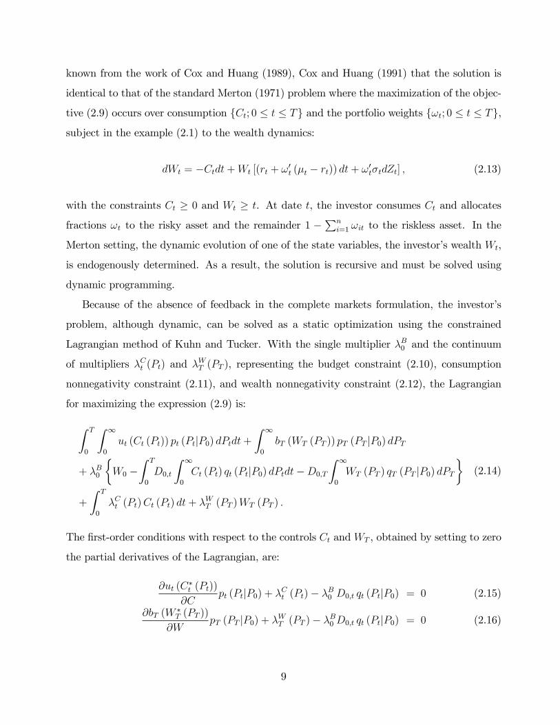
known from the work of Cox and Huang (1989), Cox and Huang (1991) that the solution is
identical to that of the standard Merton (1971) problem where the maximization of the objec-
tive (2.9) occurs over consumption fCt; 0 � t � Tg and the portfolio weights f!t; 0 � t � Tg,
subject in the example (2.1) to the wealth dynamics:
dWt = �Ctdt+Wt [(rt + !0t (�t � rt)) dt+ !0t�tdZt] ; (2.13)
with the constraints Ct � 0 and Wt � t. At date t, the investor consumes Ct and allocates
fractions !t to the risky asset and the remainder 1 �Pn
i=1 !it to the riskless asset. In the
Merton setting, the dynamic evolution of one of the state variables, the investor�s wealth Wt,
is endogenously determined. As a result, the solution is recursive and must be solved using
dynamic programming.
Because of the absence of feedback in the complete markets formulation, the investor�s
problem, although dynamic, can be solved as a static optimization using the constrained
Lagrangian method of Kuhn and Tucker. With the single multiplier �B0 and the continuum
of multipliers �Ct (Pt) and �WT (PT ), representing the budget constraint (2.10), consumption
nonnegativity constraint (2.11), and wealth nonnegativity constraint (2.12), the Lagrangian
for maximizing the expression (2.9) is:
Z T
0
Z 1
0
ut (Ct (Pt)) pt (PtjP0) dPtdt+Z 1
0
bT (WT (PT )) pT (PT jP0) dPT
+ �B0
�W0 �
Z T
0
D0;t
Z 1
0
Ct (Pt) qt (PtjP0) dPtdt�D0;T
Z 1
0
WT (PT ) qT (PT jP0) dPT�
+
Z T
0
�Ct (Pt)Ct (Pt) dt+ �WT (PT )WT (PT ) :
(2.14)
The �rst-order conditions with respect to the controls Ct and WT , obtained by setting to zero
the partial derivatives of the Lagrangian, are:
@ut (C�t (Pt))
@Cpt (PtjP0) + �Ct (Pt)� �B0 D0;t qt (PtjP0) = 0 (2.15)
@bT (W�T (PT ))
@WpT (PT jP0) + �WT (PT )� �B0 D0;t qt (PtjP0) = 0 (2.16)
9

and the �rst-order conditions with respect to the multipliers are:
�Ct (Pt)C�t (Pt) = 0
�WT (PT )W�T (PT ) = 0 (2.17)
�B0
�W0 �
Z T
0
D0;t
Z 1
0
C�t (Pt) qt (PtjP0) dPtdt�D0;T
Z 1
0
W �T (PT ) qT (PT jP0) dPT
�= 0:
Since @ut=@C > 0 and @bT=@W > 0; the investor is unsatiated for both consumption and
bequests. As a result, �B0 > 0 and the budget constraint (2.10) is binding. Solving the �rst
order conditions (2.15)-(2.16) for the multipliers �Ct and �Wt yields:
�Ct (Pt) = max
�0; �B0 D0;t qt (PtjP0)�
@ut (0)
@Cpt (PtjP0)
�(2.18)
�WT (PT ) = max
�0; �B0 D0;t qt (PtjP0)�
@bT (0)
@WpT (PT jP0)
�; (2.19)
where the max operators re�ect the fact that the multipliers are non-zero only when the
corresponding choice variables are zero.
Since @2ut=@C2 < 0 and @2bT=@W 2 < 0; the inverse functions (@ut=@C)�1(@ut=@C) =
C and (@bT=@W )�1(@bT=@W ) = W are well-de�ned for all C � 0 and W � 0 and are
strictly decreasing. Solving the �rst order conditions (2.15)-(2.16), given the budget constraint
multiplier �B0 ; yields the optimal policies:
C�t (Pt) = max
"0;
�@ut@C
��1��B0 D0;t
qt (PtjP0)pt (PtjP0)
�#(2.20)
W �T (PT ) = max
"0;
�@bT@W
��1��B0 D0;T
qT (PT jP0)pT (PT jP0)
�#; (2.21)
where here the max operators re�ect the fact that either C�t (Pt) = 0 or C�t (Pt) > 0; but in
the latter case �Ct (Pt) = 0, and similarly for W�T (PT ) and �
WT (PT ).
From equations (2.20)-(2.21), the optimal policies are fully characterized once the (scalar)
budget constraint multiplier �B0 is determined. Since non-satiation implies that the budget
10

constraint is binding, plugging the optimal policies (2.20)-(2.21) into equation (2.10) yields:
W0 =
Z T
0
D0;t
Z 1
0
max
"0;
�@ut@C
��1��B0 D0;t
qt (PtjP0)pt (PtjP0)
�#qt (PtjP0) dPtdt
+D0;T
Z 1
0
max
"0;
�@bT@W
��1��B0 D0;T
qT (PT jP0)pT (PT jP0)
�#qT (PT jP0) dPT
; (2.22)
which determines �B0 : Replacing �B0 by its value in equations (2.20)-(2.21) completes the
characterization of the investor�s optimal policies.
In the special but popular case of constant relative risk aversion (CRRA) utility with
ut(C) = �tC1� =(1� ) and bT (W ) = �TW 1� =(1� ), the inverse functions are:
�@ut@C
��1(u) =
��t
u
�1= and
�@ut@C
��1(b) =
��t
b
�1= : (2.23)
The budget constraint (2.22) therefore reduces to W0 =��B0��1=
I0 with:
I0 �Z T
0
D0;t
Z 1
0
max
"0;
�@ut@C
��1�D0;t
qt (PtjP0)pt (PtjP0)
�#qt (PtjP0) dPtdt
+D0;T
Z 1
0
max
"0;
�@bT@W
��1�D0;T
qT (PT jP0)pT (PT jP0)
�#qT (PT jP0) dPT :
(2.24)
Moreover, the optimal policies can be written in terms of the consumption to initial wealth
and terminal wealth to initial wealth ratios as:
C�t (Pt)
W0
=1
I0max
"0; �t=
�D0;t
qt (PtjP0)pt (PtjP0)
��1= #(2.25)
W �T (PT )
W0
=1
I0max
"0; �t=
�D0;T
qT (PT jP0)pT (PT jP0)
��1= #: (2.26)
2.5 Relative Price Di¤erences vs. Consumption Smoothing
Equations (2.25)-(2.26), or their more general versions (2.20)-(2.21), illustrate the trade-o¤
that is the economic essence of optimal portfolio and consumption choice. On one hand, the
investor wants to consume more in states in which the price of consumption is cheap relative
11

to the probability of realizing these states (choose a higher C�t when the ratio qt=pt is low).
This e¤ect tends to make the investor�s optimal consumption path respond to changes in the
asset prices, because as Pt changes, so does qt=pt: On the other hand, deviations across states
from a constant value C�t = C� are penalized by the investor�s risk aversion. The higher ,
the more the investor wants to smooth consumption across states and the less sensitive C�t
becomes to variations in qt=pt: In the limit as !1; the optimal policy becomes C�t = C�,
irrespectively of the price of consumption in di¤erent states.
2.6 Portfolio Implementation of the Optimal Investment Policy
Once the optimal state contingent consumption and bequest plan has been determined, this
plan can be implemented at date 0 by purchasing pure Arrow-Debreu securities. Speci�cally,
to implement the optimal consumption plan, the investor purchases for every state P at each
future date t a quantity C�t (P ) dt of Arrow-Debreu securities paying $1 if Pt = P and 0
otherwise. In addition, the investor buys quantities W �T (P ) of Arrow-Debreu securities for
states P at the terminal date T , to implement the optimal bequest plan.
Arrow-Debreu securities can be synthesized or at least approximated closely by butter�y
strategies involving plain vanilla European call options on the underlying assets. Consider the
following butter�y strategy payo¤:
Xt (Pt;K; ") =max [0; Pt �K + "] + max [0; Pt �K � "]� 2max [0; Pt �K]
"2; (2.27)
formed using European call options with strike prices K � " < K < K + ". A security with
this payo¤ converges to an Arrow-Debreu security at P = K in the limit as "! 0. It follows
immediately that the optimal consumption and bequest plan can be implemented by trading
a basket of European call options on the underlying assets.
In case the required call options are not directly available in a liquid market, they can
themselves be replicated by a dynamic trading strategy in the underlying assets. It is precisely
this replicating strategy in the underlying assets which most of the portfolio choice literature
focuses on. The economic point of the preceding discussion is that, in our complete markets
framework, the optimal portfolio choice is fully characterized by the optimal state contingent
12

consumption and bequest plan. As a result, the remainder of the paper focuses on the latter
economic decision.
3. Option-Implied State Price Density q
The previous section showed that the optimal state contingent consumption and bequest
plan as well as its trading implementation are fully determined by functions of the state-
price densities qt(PtjP0) and the physical transition densities pt(PtjP0). We now discuss how
to characterize empirically these two objects, starting with the state-price densities qt. In a
nutshell, we use data on exchange traded European put and call options to infer the state-
price densities using a parametric multivariate counterpart to the nonparametric univariate
method described in Aït-Sahalia and Lo (1998).
3.1 Marginal SPD for Each Asset Class
Consider �rst the case of a single risky asset and assume initially that the asset price Pt
is distributed log-normal under the measure Qt with a mean of EQt0 [Pt] and a volatility of
log returns ln(Pt)� ln(P0) equal to �0;tpt. We refer to this model as the Black-Scholes case,
although in the standard Black-Scholes model Pt is log-normal under the single risk-neutral
measure RN , as opposed to the sequence of measures Qt.4 De�ne the yield of a zero-coupon
bond with maturity date t to be Y0;t; so that D0;t = exp(�Y0;tt):
Let H denote the price of a European call option with maturity date t and strike price K,
given by equation (2.5) evaluated for the payo¤ function Xt(Pt) = max (Pt �K; 0). Under
the Black-Scholes assumptions, we have:
HBS(P0; K; t; �0;t) = D0;t EQt0 [max (Pt �K; 0)]
= D0;t (F0;t�(d1)�K�(d2)) ;(3.1)
4Under the Black-Scholes assumption of a constant interest rate, rt = r, which we do not adopt here, thetwo sets of measures are identical.
13

with
d1 �ln (F0;t=K)
�0;tpt
+1
2�0;tpt and d2 � d1 � �0;t
pt: (3.2)
F0;t denotes the price of a forward contract for delivery of the asset at time t, which, using
equation (2.5), equals the expected future spot price under the measure Qt. If the asset pays
income at a rate of �0;t, this forward price is F0;t = EQt0 [Pt] = P0 exp((Y0;t � �0;t)t).
The state price density qt in the Black-Scholes case is given by:
qBS;t(PtjP0) =1
Ptp2�t�0;t
exp
��ln (Pt=P0)� (Y0;t � �0;t � �20;t=2)t
�22 t �20;t
!(3.3)
and the corresponding physical transition density pt is:
pBS;t(PtjP0) =1
Ptp2�t�0;t
exp
��ln (Pt=P0)� (�0;t � �20;t=2)t
�22 t �20;t
!; (3.4)
where �0;t denotes the expected rate of return on the asset between times 0 and t. This
expected rate of return is de�ned indirectly by the equation E0 [Pt] = P0 exp(�0;t t):
Suppose now, as is the overwhelmingly common assumption in practice, that the call
pricing function is given by the Black-Scholes formula (3.1), except that the volatility para-
meter for a given option is determined by a function �0;t = �0(K=F0;t; t) of the moneyness
M0;t � K=F0;t and time-to-maturity t of the option:
H(P0; K; t) = HBS(P0; K; t; �0(K=F0;t; t)): (3.5)
Applying the basic pricing equation (2.5) to this far more general case yields:
H(P0; K; t) = D0;t EQt0 [max (Pt �K; 0)] = D0;t
Z +1
K
(Pt �K) qt (PtjP0) dPt: (3.6)
Following Banz and Miller (1978) and Breeden and Litzenberger (1978), the state price density
can then be recovered by direct di¤erentiation:
qt (KjP0) =1
D0;t
@2H
@K2(P0; K; t); (3.7)
14

where the total derivatives account for the dependence of the function �0(K=F0;t; t) on K:
@H
@K=@HBS@K
+1
F
@�0@M
@HBS@�
@2H
@K2=@2HBS@K2
+2
F
@�0@M
@2HBS@K@�
+1
F 2
�@�0@M
�2@2HBS@�2
+1
F 2@2�
@M2
@HBS@�
:
(3.8)
Aït-Sahalia and Lo (1998) exploit this equation to infer an estimate of qt from a non-parametric
estimate of the second partial derivative of the call pricing function with respect to the strike
price. We follow a similar approach, except that we parametrically model the volatility func-
tion �0(K=F0;t; t). We discuss our speci�c modelling choice in the context of the empirical
application.
3.2 Joint SPD for Two Asset Classes
We now extend this idea to two assets, say stocks and bonds, with price vector Pt =
(P1t; P2t)0: The price of a call option written on the �rst asset is, again from equation (2.5):
H1(P0; K; t) = D0;t
Z +1
0
Z +1
K
(P1t �K) qt (PtjP0) dP1tdP2t
= D0;t
Z +1
K
(P1t �K) q1t (P1tjP0) dP1t;(3.9)
where we denote by q1t (P1tjP0) the marginal state price density:
q1t (P1tjP0) =Z +1
0
qt (P1t; P2tjP0) dP2t: (3.10)
Applying the univariate procedure described in the previous section to options on the �rst
asset alone therefore allows us to estimate q1t (P1tjP0). Similarly, the marginal state price
density q2t (P2tjP0) can be estimated from options on the second asset alone.
To obtain a joint distribution from the two marginal densities, it is convenient to �rst
transform variables from prices to log returns. Let Rt denote the annualized log return implied
by the prices Pt. The two are related by the deterministic change of variable Pt = P0 exp(t Rt),
15

so that the density of returns is given by the Jacobian formula:
qt (RtjP0) = t P0 exp(Rt) qt (PtjP0) : (3.11)
Since there is no risk of confusing the densities of prices and returns, we do not distinguish
the notation between the two. The argument (Pt or Rt) indicates which is which.
We assume that the joint state price density qt (RtjP0) implied by the two marginal state
price densities is of the Plackett (1965) form.5 Speci�cally, we assume that the joint cumulative
distribution function (CDF):
Qt (RtjP0) =Z Rt
qt (RtjP0) dRt (3.12)
is given by:
Qt (RtjP0) =�At (RtjP0)2 + 4� (1� �)Q1t (R1tjP0)Q2t (R2tjP0)
1=2 � At (RtjP0)2 (1� �) ; (3.13)
where Q1t and Q2t are the CDFs corresponding to the marginal densities q1t and q2t; and:
At (RtjP0) = 1� (1� �) fQ1t (R1tjP0) +Q2t (R2tjP0)g : (3.14)
The Plackett family is parameterized by �, which controls the correlation between the two
variables R1t and R2t: In particular, � = 0 corresponds to a correlation � = �1, � = 1 to a
correlation � = 0, and lim�!+1 to a correlation � = 1: In the special case of � = 1; which
yields uncorrelated variables, equation (3.13) turns into:
Qt (RtjP0) = Q1t (R1tjP0)Q2t (R2tjP0) : (3.15)
In our empirical application, we calibrate the parameter � to the historical correlation of log
returns over horizon t.6 Finally, given the joint CDF (3.12) from the Plackett formula, we
5See Rosenberg (2003) for another use of the Plackett family of densities with given marginal densities.6By Girsanov�s Theorem, the second moments are una¤ected by the change of measure in the continuous-
time limit, and approximately so at �nite horizons. This justi�es using the empirical correlation as a proxy
16
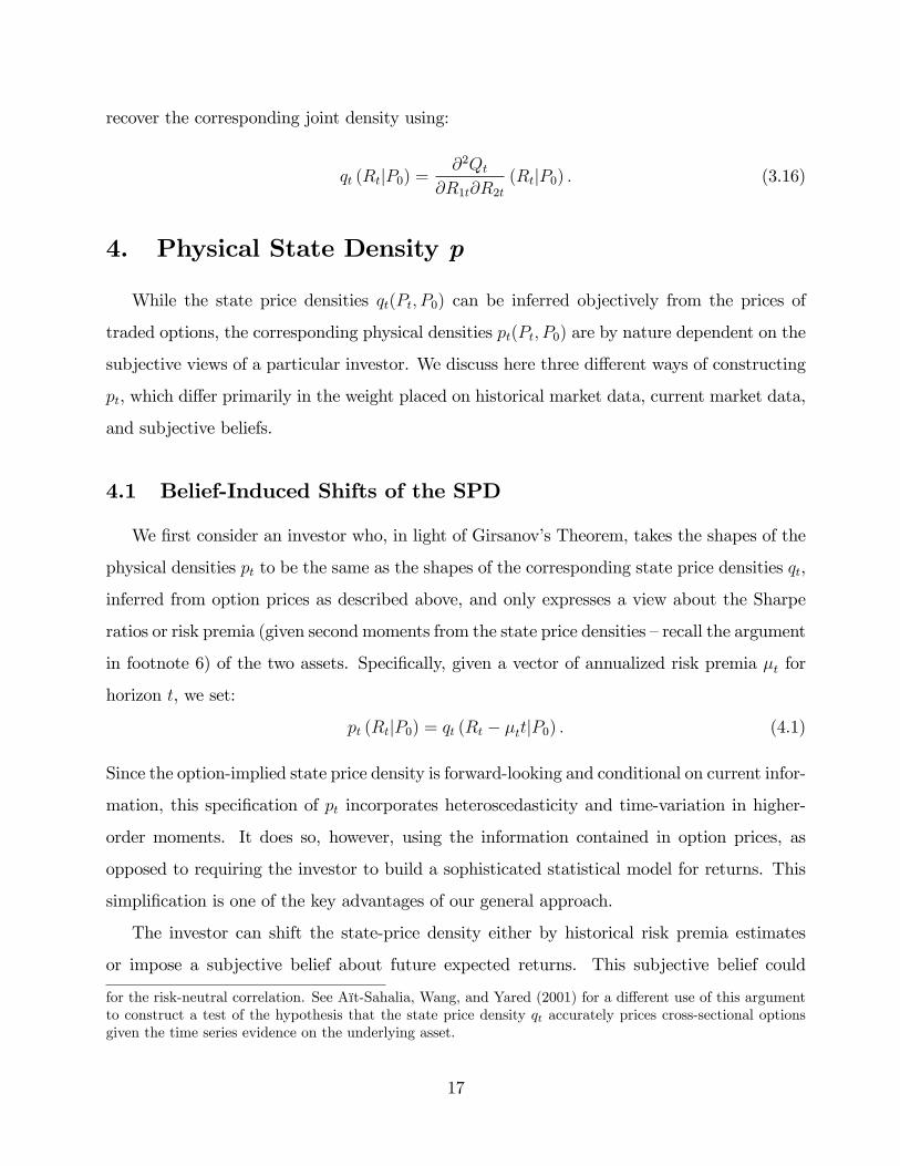
recover the corresponding joint density using:
qt (RtjP0) =@2Qt
@R1t@R2t(RtjP0) : (3.16)
4. Physical State Density p
While the state price densities qt(Pt; P0) can be inferred objectively from the prices of
traded options, the corresponding physical densities pt(Pt; P0) are by nature dependent on the
subjective views of a particular investor. We discuss here three di¤erent ways of constructing
pt, which di¤er primarily in the weight placed on historical market data, current market data,
and subjective beliefs.
4.1 Belief-Induced Shifts of the SPD
We �rst consider an investor who, in light of Girsanov�s Theorem, takes the shapes of the
physical densities pt to be the same as the shapes of the corresponding state price densities qt,
inferred from option prices as described above, and only expresses a view about the Sharpe
ratios or risk premia (given second moments from the state price densities �recall the argument
in footnote 6) of the two assets. Speci�cally, given a vector of annualized risk premia �t for
horizon t, we set:
pt (RtjP0) = qt (Rt � �ttjP0) : (4.1)
Since the option-implied state price density is forward-looking and conditional on current infor-
mation, this speci�cation of pt incorporates heteroscedasticity and time-variation in higher-
order moments. It does so, however, using the information contained in option prices, as
opposed to requiring the investor to build a sophisticated statistical model for returns. This
simpli�cation is one of the key advantages of our general approach.
The investor can shift the state-price density either by historical risk premia estimates
or impose a subjective belief about future expected returns. This subjective belief could
for the risk-neutral correlation. See Aït-Sahalia, Wang, and Yared (2001) for a di¤erent use of this argumentto construct a test of the hypothesis that the state price density qt accurately prices cross-sectional optionsgiven the time series evidence on the underlying asset.
17

be formed through a forecasting model, professional investment advice, introspection, or a
combination thereof.7 Notice that in the limiting case where the investor believes that the
risk premia are zero (so pt = qt), the optimal policies are state-independent, since equations
(2.20)-(2.21) reduce to:
C�t (Pt) = max
"0;
�@ut@C
��1 ��B0 D0;t
�#(4.2)
W �T (PT ) = max
"0;
�@bT@W
��1 ��B0 D0;T
�#: (4.3)
4.2 Gaussian Density
We also consider the case of Gaussian physical densities:
pt (RtjP0) = N [(Y0;t + �t) t;�tt] (4.4)
where the vector of annualized risk premia �t and the annualized return covariance matrix �t
for horizon t are both speci�ed by the investor, and whereN [a; b] denotes the Gaussian density
with mean a and variance b. One possible justi�cation for this relatively simple speci�cation
of pt is that a typical investor, already �nding it challenging to form views about the �rst
two moments of returns, is unlikely to be willing or able to express strong beliefs about
the skewness, kurtosis, and higher order moments of the (log) return density. The investor
therefore defaults to the intuitive and theoretically appealing Black-Scholes benchmark case
discussed above.
As in the case of belief-induced shifts of the state price density, the moments �t and
�t of the Gaussian density can be based on a forecasting model, professional investment
advice, introspection, or a combination thereof. Alternatively, the covariance matrix �t can
be calibrated, again in light of Girsanov�s Theorem, to the second moments of the state price
density, which leaves only the risk premia to be speci�ed by investor. In the tables and �gures
below, we will express views directly on the Sharpe ratios of the two assets.
7For instance, risk premia can be calibrated to the consensus forecasts by the academic �nance professionor by Chief Financial O¢ cers, as reported in Welch (2000) and Graham and Harvey (2002), respectively.
18

4.3 Empirical Density
Finally, an obvious case can be made for using historical data as the basis for constructing
the physical density pt. Given a time series of realized log returns over horizon t, R1;t;s and
R2;t;s, for s = 1; :::; S, we construct for each asset a histogram of the marginal physical distri-
bution pit (PitjPi0) or a smoothed version of it in the form of a kernel density estimator.8 We
then obtain the joint physical density pt (PtjP0) by combining the two marginal densities using
the Plackett formula described in the previous section. The parameter � is again calibrated
to the historical correlation of log returns at horizon t.
In order to focus on the shape of the physical densities, we rescale in our application the
empirical densities to have the same second moments as the state-price densities and shift
them according to views on the Sharpe ratios of the two assets. The only di¤erence between
using empirical densities and the other two cases discussed above is that the shape of the
empirical densities is by construction backward-looking and unconditional. In contrast, the
shape of the state-price densities is forward-looking and conditional on current information.
5. Empirical Implementation
We now implement our approach empirically. We use option prices to infer the state price
densities qt; and then examine the optimal consumption policies corresponding to the di¤erent
choices of the physical state densities pt described above. Besides illustrating the mechanics of
our approach, the contribution of this application is two-fold. First, we investigate empirically
the trade-o¤ between exploiting di¤erences in the prices of consumption in di¤erent states
and smoothing consumption across states, for di¤erent choices of the physical state density.
Second, we illustrate the tension between the state prices inferred from option prices and the
beliefs expressed in the risk premium surveys mentioned above. One can view this tension as
another take on the equity premium puzzle.
We consider an individual who can invest in two risky securities, a stock fund that tracks
the S&P 500 index and a bond fund with duration equal to that of a 10-year Treasury note
8See, for example, Wand and Jones (1995) for a description of kernel density estimation techniques.
19

futures, in addition to the risk-free money market account. We solve for the optimal con-
sumption policies assuming the investor has CRRA preferences with = 5 and � = 0:98. For
simplicity, we abstract from the bequest motive by assuming bT (WT ) = 0.
Although we focus on CRRA preferences in this application, it is clear from the theory
that our approach can be applied just as easily to any other choice of preferences. Given
estimates of qt and pt, the optimal consumption choice is characterized by equation (2.20),
which simpli�es to equation (2.25) in the case of CRRA preferences. The estimation of the
densities is independent of the investor�s preferences. It follows that the relative prices of
consumption in di¤erent states, which depend only on the ratio qt=pt, are also una¤ected
by the preferences. The only role played by the utility function (its inverse actually) is the
relative desire of the investor to smooth consumption across dates and states.
5.1 Data
We collect options data for the S&P 500 index (SPX) and the 10-year Treasury note futures
(TY). The SPX options are traded at the Chicago Board Options Exchange (CBOE) and the
TY options are traded at the Chicago Board of Trade (CBOT). Both are extremely liquid,
with aggregate daily volumes well in excess of 100,000 contracts each. For 10 consecutive days
(January 6�17, 2003) we obtain the bid and ask quotes of all listed SPX and TY options at
11:30 am. We then take the price of each option to be the midpoint between the bid and
ask quotes. Finally, we compute implied volatilities from these mid-point prices using the
prevailing term structure of Eurodollar interest rates. Table 1 describes the options data.
We also collect daily closing prices of the S&P 500 index and the on-the-run 10-year
Treasury note from January 2, 1962 through January 17, 2003. We use this data to compute
the historical moments and the joint empirical densities of the stock and bond returns at
di¤erent horizons. Table 2 describes the underlying asset data.
5.2 Density Estimation
We use the raw options data to infer �rst the marginal and ultimately the joint state
price densities for the S&P 500 index and 10-year Treasury bond. The SPX option contract
20

is European style, as required by our econometric approach. The TY option contract, in
contrast, is American style, allowing for early exercise prior to expiration. The underlying
asset of the TY contrast is a 10-year Treasury note futures contract; see Fama and French
(1988) for an adjustment for the early exercise premium, and the construction of an equivalent
European option.
In-the-money options are notoriously illiquid and their prices can be unreliable. We there-
fore replace the in-the-money option prices with ones implied by put-call-parity and more
liquid out-of-the-money options. Given a European call option price H(Pi0; K; t), put-call-
parity yields the European put option price L(Pi0; K; t) for the same strike price and maturity
date:
H(Pi0; K; t)� L(Pi0; K; t) = D0;t
�EQt0 [Pit]�K
�: (5.1)
We �rst evaluate put-call parity at the money (K ' Pi0), where both the call and put are
the most liquid, to obtain a common implied forward price Fi0 = EQt0 [Pit].
9 We then apply
this option-implied forward price to put-call-parity for all away-from-the-money strike prices
to replace the illiquid in-the-money option prices with liquid out-the-money ones.
We next invert each option price to an implied volatility, using the at-the-money option-
implied forward price of the underlying asset, and �t a standard parametric implied volatil-
ity surface (the so-called �practitioner Black-Scholes model") by constrained ordinary least
squares. Speci�cally, we model the implied volatilities for the S&P 500 index as:
�0(K=F10;t; t) = 0:696� 0:308 (K=F10;t)� 0:175 t+ 0:132 (K=F10;t) t if t � 2:5
= 0:259 (the �tted value for t = 2:5) if t > 2:5;(5.2)
and the implied volatilities for the 10-year Treasury note futures as:
�0(K=F20;t; t) = 0:356� 0:265 (K=F20;t)� 0:158 t+ 0:265 (K=F20;t) t if t � 1:0
= 0:197 (the �tted value for t = 1:0) if t > 1:0:(5.3)
The implied volatility surface is constrained to be �at, with continuous �rst and second deriv-
9The forward price is the value Fi0;t that solves D0;t EQt
0 [Pit � Fi0;t] = 0:
21

atives, at a horizon of 2.5 years for the S&P 500 index and one year for the 10-year Treasury
note futures. The reason for these constraints is that liquid options are not available beyond
these maturities. The constraints e¤ectively set the implied volatilities for longer horizons
equal to the implied volatilities of the longest available at-the-money options. The model
speci�cations �t the data well, with multiple R2 equal to 95.5% for the S&P 500 index and
79.5% for the 10-year Treasury note futures options.
The advantage of these simple parametric models is that the partial derivatives needed for
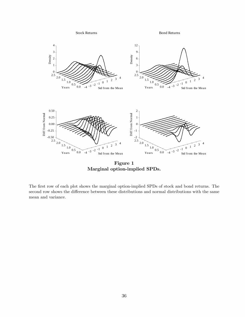
equation (3.8) can be evaluated analytically.10 Figure 1 plots the resulting marginal SPDs qt
for horizons t ranging from one to 10 quarters (2.5 years). The �gure also shows deviations of
the SPDs from Gaussian densities with the same mean and variance (i.e., their Black-Scholes
counterparts). All densities are plotted in terms of standardized (log) returns. By now it
is well understood that options data with negatively sloped implied volatility surfaces, as
in equations (5.2) and (5.3), correspond to negatively skewed and leptokurtic SPDs qt (see
Aït-Sahalia and Lo (1998)).
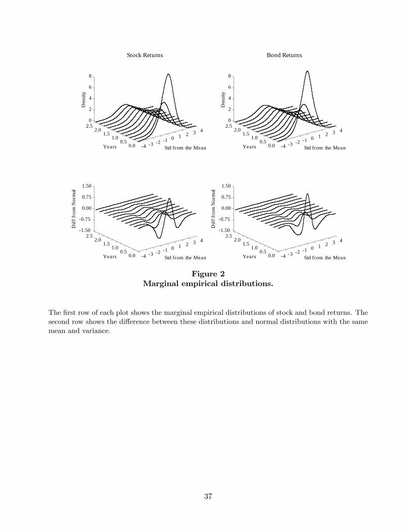
For comparison, we compute kernel estimates of the empirical marginal densities pt using
the historical returns data. Figure 2 presents the results for the same horizons as in Figure 1
above. Just as we constrained the option-implied SPDs for the log-returns to be Gaussian at
long horizons, we constrain the empirical densities to also be Gaussian at the same horizons of
2:5 and one year for stocks and bonds, respectively. Since the optimal solution for a horizon
t depends on the ratio qt=pt at that horizon, the impact of this constraint is limited to the
constant of proportionality I0, which in turn does not distort the optimal choice because it
a¤ects all states and dates equally.
There are two striking di¤erences between the two sets of densities. First, while both
exhibit pronounced di¤erences from normal distributions (see the second row of plots), the
non-normalities of the empirical densities are much more concentrated toward short horizons
than for the SPDs. This is especially the case for stocks, where the distribution of one-year
returns is roughly as non-normal as the distribution of one-month returns. Empirically, in
contrast, one-year returns are nearly Gaussian. Second, consistent with the literature, both
10Alternatively, a fully nonparametric �t is possible even with a single day�s worth of option data if theappropriate model-free no-arbitrage shape restrictions are imposed, see Aït-Sahalia and Duarte (2003).
22

SPDs are considerably more negatively skewed than the empirical densities.
The next step is to use the Plackett formula to combine the marginal densities into joint
densities. This requires that we �rst calibrate the coe¢ cient � in equation (3.13) to the
estimated correlation of the stock and bond returns at di¤erent horizons t for each set of
marginal densities. Table 3 gives details on this calibration. The second column of the table
reports the empirical correlation between stock at bond returns at horizons ranging from one
day to one year. The remaining columns provide the values of the coe¢ cient � for which
the correlation implied by the resulting Plackett density matches the empirical correlation.
Columns three, four, and �ve correspond to the option-implied SPDs q; the empirical densities
p; and Gaussian densities p, respectively.
Figure 3 illustrates the relationship between the coe¢ cient � of the Plackett copula and
the implied correlation � of stock and bond returns. The four lines in each plot correspond
to return horizons of one month (solid), one quarter (dashed), one year (dashed-dotted), 2.5
years (dotted). The left plot is for the option-implied densities and the right plot is for the
historical empirical densities. Since the marginal densities in both cases are constrained to
be Gaussian at the 2.5-year horizon, the relationship between � and � for Gaussian returns
(at any horizon) is illustrated by the dotted line in either plot. The main message of this
�gure is that the calibrated values of � are remarkably stable across di¤erent shapes of the
marginal densities. As a result, our empirical results below are relatively insensitive to this
intermediate calibration of the Plackett formula.
We can now combine these inputs to produce, at last, the objects of economic interest.
Figures 4 and 5 present contour plots at horizons of one month, one quarter, one year, and
2.5 years of the joint option-implied and historical empirical densities, respectively. The joint
densities are constructed by combining the marginal densities through the Plackett formula.
Each contour corresponds to 10 percent cumulative probability. As expected from the marginal
densities in Figure 1 and 2, the joint option-implied densities in Figure 4 exhibit substantially
more non-normality than the empirical ones in Figure 5.
23

5.3 Relative Prices of Consumption
Given estimates of the option-implied SPDs qt at di¤erent horizons, shown in Figure 4, we
can use equation (2.25) to compute the consumption and portfolio rules of a CRRA investor for
the various choices of the physical state density pt, one of them being the historical empirical
density in Figure 5. As we discussed in Section 2.4, the solution can interpreted in two
parts. First, the investor wants to consume more in states in which the price of consumption
is cheap relative to the probability of realizing these states. Second, the investor wants to
smooth consumption across states. In this section, we �rst examine the relative price e¤ect,
which is independent of the investor�s preferences and is captured by the ratio qt=pt. In Section
5.4, we then examine the smoothing e¤ect, which for CRRA preferences depends also on the
coe¢ cient of relative risk aversion .
Before exploring other possibilities, we present in Figure 6 as benchmark the ratio qt=pt
under log-normality, corresponding to the Black-Scholes economy discussed above. The four
plots show the relative prices of consumption in one month, one quarter, one year, and 2.5
years into the future. The SPD qt is log-normal with moments matching the option-implied
SPD. The physical distribution pt is equal to the log-normal SPD shifted by risk premia that
imply annualized Sharpe ratios of 0.5 for stocks and 0.05 for bonds (roughly in line with the
historical moments reported in Table 2). We use these particular risk premia beliefs here and
below not to advocate them as the best forecasts of future excess returns, but rather in order
to focus the comparison between di¤erent cases on the shapes of the densities, rather than on
their location.11 In this �gure and the following, we classify states (i.e., the joint realizations of
returns for stocks and bonds) in terms of number of standard deviations from their respective
SPD means.
The shading in the plot signi�es the relative prices of consumption, with the black area
as the most expensive states and the white area as the cheapest states. The legends next
to each plot provide a rough scale of the relative price di¤erences. For example, at the one
month horizon, consumption in the black states is approximately 1:16=0:86 = 1:34 times as
11In fact, most estimates of the current equity risk premium are well below the historical equity risk premium.Fama and French (2001) estimate the equity risk premium to lie between 2.5% and 4.3%. Ibbotson and Chen(2003) estimate it to be between 4.0% and 6.0% at long horizons.
24

expensive as consumption in the white states.
To get a more precise reading of the relative prices of consumption, we tabulate in Table
4 the ratio qt=pt for nine states (all permutations of the bond and stock returns equal to their
means and to their means plus or minus 1.5 standard deviations). For each state, the table
shows a block of four numbers. The results for the benchmark case of log-normality are shown
in the �rst row of each block.
At least three broad patterns emerge from Figure 6 and Table 4. First, consumption is
most expensive in states associated with negative bond and stock returns, and it is cheapest
in states associated with positive bond and stock returns. This pattern is consistent with the
fact that both assets demand a positive risk premium. Second, the relative price gradient is
considerably steeper across stock return states than bond return states, in line with the equity
risk premium being substantially higher than the bond risk premium. Third, the spread be-
tween the cheapest and most expensive consumption states increases with the return horizon.
This pattern is generated by the fact that both risk premiums increase approximately linearly
with the return horizon (the e¤ect is not exactly linear because of the di¤erent annualized
risk premiums across horizons shown in Table 2).
Instead of assuming log-normality, we now combine the option-implied SPD qt with each
of the three di¤erent physical state densities pt discussed in Section 4. We �rst construct pt
by shifting the option-implied SPD by risk premia that imply annualized Sharpe ratios of 0.5
for stocks and 0.05 for bonds. Figure 7 and the second row in each block of numbers in Table
4 report the ratios of the two densities, qt=pt, for this case. Notice that the results for the 2.5
year horizon are the same as for log-normality since we force the option-implied state price
density to be log-normal beyond horizons for which options data is available.
The three broad patterns we discussed for the log-normal benchmark case are also clearly
apparent with the option-implied distributions. There are, however, at least two important
di¤erences in the results. First, with the option-implied distributions the ratio qt=pt is lower
for extreme stock return states and higher for extreme bond return states. The di¤erence
in qt=pt for the option implied distribution relative to log-normality is most pronounced for
extreme positive stock return states, which means that the di¤erences between extreme states
increases considerably.
25
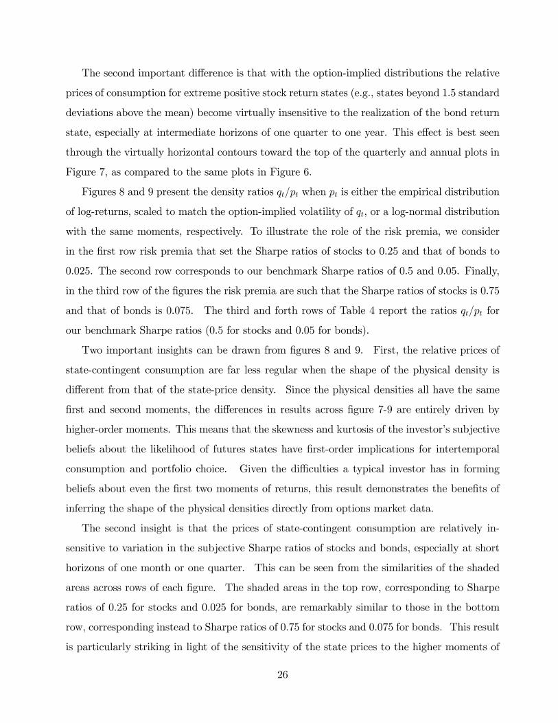
The second important di¤erence is that with the option-implied distributions the relative
prices of consumption for extreme positive stock return states (e.g., states beyond 1.5 standard
deviations above the mean) become virtually insensitive to the realization of the bond return
state, especially at intermediate horizons of one quarter to one year. This e¤ect is best seen
through the virtually horizontal contours toward the top of the quarterly and annual plots in
Figure 7, as compared to the same plots in Figure 6.
Figures 8 and 9 present the density ratios qt=pt when pt is either the empirical distribution
of log-returns, scaled to match the option-implied volatility of qt, or a log-normal distribution
with the same moments, respectively. To illustrate the role of the risk premia, we consider
in the �rst row risk premia that set the Sharpe ratios of stocks to 0.25 and that of bonds to
0.025. The second row corresponds to our benchmark Sharpe ratios of 0.5 and 0.05. Finally,
in the third row of the �gures the risk premia are such that the Sharpe ratios of stocks is 0.75
and that of bonds is 0.075. The third and forth rows of Table 4 report the ratios qt=pt for
our benchmark Sharpe ratios (0.5 for stocks and 0.05 for bonds).
Two important insights can be drawn from �gures 8 and 9. First, the relative prices of
state-contingent consumption are far less regular when the shape of the physical density is
di¤erent from that of the state-price density. Since the physical densities all have the same
�rst and second moments, the di¤erences in results across �gure 7-9 are entirely driven by
higher-order moments. This means that the skewness and kurtosis of the investor�s subjective
beliefs about the likelihood of futures states have �rst-order implications for intertemporal
consumption and portfolio choice. Given the di¢ culties a typical investor has in forming
beliefs about even the �rst two moments of returns, this result demonstrates the bene�ts of
inferring the shape of the physical densities directly from options market data.
The second insight is that the prices of state-contingent consumption are relatively in-
sensitive to variation in the subjective Sharpe ratios of stocks and bonds, especially at short
horizons of one month or one quarter. This can be seen from the similarities of the shaded
areas across rows of each �gure. The shaded areas in the top row, corresponding to Sharpe
ratios of 0.25 for stocks and 0.025 for bonds, are remarkably similar to those in the bottom
row, corresponding instead to Sharpe ratios of 0.75 for stocks and 0.075 for bonds. This result
is particularly striking in light of the sensitivity of the state prices to the higher moments of
26

the physical densities (comparing Figure 7 to the middle rows of �gures 7-9).
5.4 Optimal Consumption Policies for Di¤erent p
Given the ratio qt=pt determined above, we now compute the optimal consumption plan,
according to equation (2.25), across di¤erent realizations of the joint returns on stocks and
bonds. Once the optimal consumption plan is determined, the investor�s optimal portfolio
strategy consists of purchasing a continuum of pure Arrow-Debreu securities. At date 0, the
investor purchases for each state P and each date t a quantity C�t (P ) dt of the Arrow-Debreu
security paying $1 if Pt = P and 0 otherwise. While not directly traded on exchanges, such
Arrow-Debreu securities can be synthesized exactly using traded European call options on the
underlying assets, or simply approximated in the form of butter�y payo¤s (which converge to
the Arrow-Debreu payo¤ if the strikes used to form the butter�y converge), as described in
Section 2.6. In other words, the optimal investment strategy is fully characterized once we
have determined the optimal consumption path.
As a benchmark for comparison, Figure 10 plots the optimal consumption of a CRRA
investor under log-normal state-price and physical densities (the Black-Scholes case) with a
risk aversion coe¢ cient ranging from 2 to 10: The plot is constructed by applying equation
(2.25) to the ratio qt=pt plotted in Figure 6. Figure 11 reports the same results when qt is
option-implied and pt is mean-shifted from qt by risk premia that imply a Sharpe ratio of 0.5
for stocks and 0.05 for bonds, corresponding to the ratio qt=pt plotted in Figure 7.
Figures 10 and 11 illustrate the trade-o¤ between exploiting di¤erences, across states, in
the relative cost of state-contingent consumption and the desire to smooth consumption across
states induced by risk aversion. As our formulation of the intertemporal problem makes clear,
this trade-o¤ is the economic essence of optimal consumption and portfolio choice. Other
things equal, the investor likes to consume more in states in which the price of consumption
is cheap relative to the (subjective) probability of realizing those states. That is, the optimal
solution selects a higher C�t when the ratio qt=pt is low. Counteracting this e¤ect, however,
deviations across states from a constant value C�t = C� are penalized by the investor�s risk
aversion. The higher ; the less sensitive C�t becomes to variations in qt=pt: In the limit,
27

as ! 1; the optimal policy becomes C�t = C� irrespectively of the relative prices of
consumption across states.
The smoothing e¤ect is quite apparent as we move in either �gure from the left column
with = 2 to the right one with = 10. As the investor�s risk aversion increases, the
regions of (approximate) constancy of consumption across states, represented by the same
shade of gray, increase. At the same time, the di¤erence in shades of gray, from lightest to
darkest, decreases Combined, these patterns imply that as risk aversion increases, more
states are associated with the same level of consumption and that the di¤erences between
consumption in the most extreme states diminishes. Risk aversion induces the investor to
smooth consumption across states.
6. Conclusions
We developed an empirical approach to solving the intertemporal consumption and portfo-
lio choice problem using option-implied information to determine the cost of consuming in, or
equivalently betting against, future states of the world. Using the martingale representation
method, we reduced the dynamic problem to a static one, in which the investor simply deter-
mines the level of state-contigent consumption in each state and at each date in the future.
Our method gives a direct role to the investor�s beliefs about the likelihood of future states,
and we proposed di¤erent ways of implementing this subjective aspect of the problem.
Our results illustrate explicitly the inherent tension between, on the one hand, the in-
vestor�s desire to exploit cross-sectional di¤erences in state prices by consuming more in states
in which the price of consumption is cheap relative to the probability of realizing these states
and, one the other hand, the desire to smooth consumption across states induced by risk
aversion. We argued that, as our formulation of the intertemporal problem makes clear, this
trade-o¤ is the economic essence of optimal consumption and portfolio choice.
Our method is potentially quite general. Unlike the dynamic programming approach to
the intertemporal consumption and portfolio choice problem, our solution is always obtained
explicitly so the numerical aspects of �nding the solution are straightforward. One limita-
tion of our method, however, is the need to be able to map future states of the world into
28

today�s cross-section of option-implied state prices. This requires that we have access to the
corresponding options data, which is a de�nite limitation especially for less standard asset
classes. That said, while we have implemented the method for the typical cash/stocks/bonds
asset allocation problem, with states of the world de�ned by the stochastic variation in the
stock and bond indices, it is certainly possible to consider more complex asset allocation prob-
lems in which the investment opportunity set further varies due randomness in the interest
rate and/or stochastic volatility. Readily available data on interest rate options and variance
swaps, respectively, make it possible to do so with our method.
29

References
Aït-Sahalia, Y., and M. Brandt, 2001, �Variable Selection for Portfolio Choice,� Journal ofFinance, 56, 1297�1351.
Aït-Sahalia, Y., and A. Lo, 1998, �Nonparametric Estimation of State-Price-Densities Implicitin Financial Asset Prices,�Journal of Finance, 53, 499�547.
Aït-Sahalia, Y., Y. Wang, and F. Yared, 2001, �Do Option Markets Correctly Price theProbabilities of Movement of the Underlying Asset?,�Journal of Econometrics, 102, 67�110.
Banz, R. W., and M. H. Miller, 1978, �Prices for State-Contingent Claims: Some Estimatesand Applications,�Journal of Business, 51, 653�672.
Breeden, D. T., and R. H. Litzenberger, 1978, �Prices of State-Contingent Claims Implicit inOption Prices,�Journal of Business, 51, 621�651.
Cox, J. C., and C.-F. Huang, 1989, �Optimum Consumption and Portfolio Policies WhenAsset Prices Follow a Di¤usion Process,�Journal of Economic Theory, 49, 33�83.
, 1991, �A Variational Problem Occurring in Financial Economics,�Journal of Math-ematical Economics, 20, 465�487.
Cvitanic, J., and I. Karatzas, 1995, �Hedging and Portfolio Optimization under TransactionCosts: Martingale Approach,�Mathematical Finance, 6, 133�165.
Detemple, J., R. Garcia, and M. Rindisbacher, 2003, �A Monte Carlo Method for OptimalPortfolios,�Journal of Finance, 58, 401�446.
Fama, E. F., and K. R. French, 1988, �The Early Exercise of Options on Treasury BondFutures,�The Journal of Financial and Quantitative Analysis, 23, 437�449.
, 2001, �The Equity Premium,�working paper, University of Chicago.
Graham, J. R., and C. R. Harvey, 2002, �Expectations of Equity Risk Premia, Volatility andAsymmetry from a Corporate Finance Perspective,�working paper, Duke University.
Harrison, M. J., and D. M. Kreps, 1979, �Martingales and Arbitrage in Multiperiod SecuritiesMarkets,�Journal of Economic Theory, 2, 381�408.
Ibbotson, R. G., and P. Chen, 2003, �Long-Run Stock Returns: Participating in the RealEconomy,�Financial Analyst Journal, Jan/Feb, 88�98.
Karatzas, I., J. P. Lehoczky, and S. E. Shreve, 1987, �Optimal Portfolio and Consumption De-cisions for a Small Investor on a Finite Horizon,�SIAM Journal of Control and Optimization,25, 1557½U1586.
Merton, R. C., 1971, �Optimum Consumption and Portfolio Rules in a Continuous-TimeModel,�Journal of Economic Theory, 3, 373�413.
30
, 1992, Continuous Time Finance. Basil Blackwell, New York, N.Y.
Plackett, R. L., 1965, �A Class of Bivariate Distributions,�Journal of the American StatisticalAssociation, 60, 516�522.
Pliska, S. R., 1986, �A Stochastic Calculus Model of Continuous Trading: Optimal Portfolios,�Mathematics of Operations Research, 11, 239½U246.
Rosenberg, J. V., 2003, �Nonparametric Pricing of Multivariate Contingent Claims,�Journalof Derivatives, 10, 9�26.
Wachter, J. A., 2002, �Portfolio and Consumption Decisions under Mean-Reverting Returns:An Exact Solution for Complete Markets,�Journal of Financial and Quantitative Analysis,37, 63�91.
Wand, M. P., and M. C. Jones, 1995, Kernel Smoothing. Chapman and Hall, London, U.K.
Welch, I., 2000, �Views of Financial Economists on the Equity Premium and on ProfessionalControversies,�Journal of Business, 73, 501�538.
31

Table 1: Options data
Mean Std Dev Min 10% 50% 90% Max
Stocks:Years to Maturity 0.8934 0.6108 0.0959 0.1753 0.7014 1.9260 1.9479Moneyness 0.9506 0.1719 0.5367 0.7535 0.9481 1.1647 1.4970Implied Volatility 0.2677 0.0426 0.1683 0.2167 0.2597 0.3284 0.4110
Bonds:Years to Maturity 0.3156 0.1837 0.0959 0.1178 0.2548 0.6767 0.7014Moneyness 1.0507 0.0621 0.9080 0.9719 1.0446 1.1375 1.2249Implied Volatility 0.1056 0.0318 0.0289 0.0616 0.1074 0.1389 0.2479
The table shows sample statistics for the options data on the S&P 500 index (stocks) and 10-yearTreasury futures (bonds). The sample period is January 6, 2003 through January 17, 2003. Theoptions prices are bid-ask midpoints recorded each day at 11:30am. There are 1093 observations forthe stock options and 600 observations for the bond options.
32

Table 2: Underlying asset data
Daily Weekly Monthly Quarterly Annual
Stocks:Mean 0.0793 0.0791 0.0794 0.0813 0.0829Volatility 0.1462 0.1586 0.1494 0.1466 0.1447Skewness -1.6958 -1.6090 -0.7071 -0.6098 -0.5969Kurtosis 47.7739 27.6679 7.1456 5.3098 3.5901
Bonds:Mean 0.0055 0.0050 0.0051 0.0062 0.0097Volatility 0.1266 0.1385 0.1487 0.1531 0.1562Skewness -0.1132 -0.2310 -0.3242 -0.3297 -0.3094Kurtosis 8.0242 6.7049 4.6273 3.6884 2.7549
Correlation -0.2262 -0.2469 -0.2526 -0.2892 -0.4004
The table shows sample statistics for the excess returns on stocks and bonds over horizons rangingfrom one day to one year. Stocks and bonds represent the S&P 500 index and the on-the-run 10-year Treasury note, respectively. Returns are measured in excess of a maturity-matched risk-freezero-coupon yield. The sample period is January 2, 1962 through January 17, 2003.
33

Table 3: Calibrating the Plackett formula to historical correlations
Calibrated �
Historical Option-Implied Physical Density ptHorizon Correlation SPD qt Empirical Gaussian
Daily -0.226 0.580 0.583 0.561Weekly -0.247 0.550 0.551 0.530Monthly -0.253 0.531 0.540 0.522Quarterly -0.289 0.446 0.473 0.464Annual -0.400 0.245 0.275 0.280
This table shows the historical correlations between stock and bond returns at di¤erent horizons. Italso shows the values of the parameter � for which the correlation implied by the Plackett formulafor the option-implied SPDs and for the empirical or Gaussian physical distributions match thecorresponding historical correlations.
34

Table 4: Relative prices of state-contingent consumption
Bond Stock Return Stock ReturnReturn �1:5 StdDev Mean +1:5 StdDev �1:5 StdDev Mean +1:5 StdDev
1 Month Horizon 1 Quarter Horizon
�1:5 2.480 0.818 0.254 1.984 1.119 0.559StdDev 3.233 1.699 0.208 1.898 1.595 0.284
0.817 1.003 0.422 0.791 0.975 0.3671.202 1.035 0.650 1.094 0.923 0.478
Mean 1.343 0.414 0.166 1.581 0.745 0.4282.368 0.869 0.135 1.711 1.105 0.2230.960 1.162 0.488 0.936 1.159 0.3990.933 0.895 0.568 1.079 0.930 0.444
+1:5 0.696 0.283 0.123 1.056 0.568 0.370StdDev 1.036 0.405 0.084 1.013 0.637 0.169
0.800 0.953 0.402 0.806 0.925 0.3141.088 1.077 0.649 1.133 0.987 0.465
1 Year Horizon 2.5 Year Horizon
�1:5 1.488 1.261 0.810 1.457 1.254 0.900StdDev 1.361 1.417 0.319 � � �
1.185 1.143 0.368 � � �1.171 1.096 0.350 � � �
Mean 1.445 0.969 0.678 1.433 1.098 0.7441.326 1.097 0.277 � � �1.251 1.047 0.214 � � �1.322 1.055 0.212 � � �
+1:5 1.178 0.556 0.659 1.283 0.854 0.728StdDev 1.073 0.846 0.271 � � �
0.954 0.830 0.206 � � �1.010 0.797 0.201 � � �
This table shows the relative prices of state-contingent consumption, measured as the ratio of theSPD and physical distribution qt=pt, for a one month, one quarter, one year, and 2.5 year horizon.There are nine states comprised of stock and bond returns equal to their mean or their mean plusor minus 1.5 standard deviations (StdDev). For each state, the table shows four rows of numbers.In the �rst row, the SPD is log-normal with moments matching the option-implied SPD and thephysical distribution is the log-normal SPD shifted by the historical risk premia. In the secondrow, the SPD is inferred from option prices and the physical distribution is the option-implied SPDshifted by the historical risk premia. In the third row, the SPD is inferred from option prices and thephysical distribution is log-normal with moments matching the option-implied SPD but shifted bythe historical risk premia. In the fourth row, the SPD is inferred from option prices and the physicaldistribution is the empirical distribution scaled to have the same moments as the option-implied SPDbut shifted by the historical risk premia.
35
4 3 2 1 0 1 2 3 4
0.00.5
1.01.5
2.02.5
0
1
2
3
4
Std from the Mean
Stock Returns
Years
Den
sity
4 3 2 1 0 1 2 3 4
0.00.5
1.01.5
2.02.5
0
3
6
9
12
Std from the Mean
Bond Returns
Years
Den
sity
4 3 2 1 0 1 2 3 4
0.00.5
1.01.5
2.02.5
0.50
0.25
0.00
0.25
0.50
Std from the MeanYears
Diff
fro
m N
orm
al
4 3 2 1 0 1 2 3 4
0.00.5
1.01.5
2.02.52
1
0
1
2
Std from the MeanYears
Diff
fro
m N
orm
al
Figure 1Marginal option-implied SPDs.
The �rst row of each plot shows the marginal option-implied SPDs of stock and bond returns. Thesecond row shows the di¤erence between these distributions and normal distributions with the samemean and variance.
36
4 3 2 1 0 1 2 3 4
0.00.5
1.01.5
2.02.5
0
2
4
6
8
Std from the Mean
Stock Returns
Years
Den
sity
4 3 2 1 0 1 2 3 4
0.00.5
1.01.5
2.02.5
0
2
4
6
8
Std from the Mean
Bond Returns
Years
Den
sity
4 3 2 1 0 1 2 3 4
0.00.5
1.01.5
2.02.5
1.50
0.75
0.00
0.75
1.50
Std from the MeanYears
Diff
fro
m N
orm
al
4 3 2 1 0 1 2 3 4
0.00.5
1.01.5
2.02.5
1.50
0.75
0.00
0.75
1.50
Std from the MeanYears
Diff
fro
m N
orm
al
Figure 2Marginal empirical distributions.
The �rst row of each plot shows the marginal empirical distributions of stock and bond returns. Thesecond row shows the di¤erence between these distributions and normal distributions with the samemean and variance.
37

4 3 2 1 0 1 2 3 4
0.8
0.6
0.4
0.2
0.0
0.2
0.4
0.6
0.8
OptionImplied SPD
ρ
ln θ4 3 2 1 0 1 2 3 4
0.8
0.6
0.4
0.2
0.0
0.2
0.4
0.6
0.8
Empirical Distribution
ρ
ln θ
Figure 3Calibrating the Plackett formula to correlations.
The plots show the relationship between the parameter � of the Plackett formula and the impliedcorrelation of stock and bond returns. The left plot is for the option-implied SPDs and the rightplot is for the empirical distributions. The solid, dashed, dashed-dotted, and dotted lines correspondto a one month, one quarter, one year, and 2.5 year horizon, respectively. In the case of Gaussiandensities, the relationship between � and � is independent of the horizon and is equal to the 2.5year case for either the option-implied or empirical distribution (since the 2.5-year distributions areconstrained to be Gaussian in all cases).
38

3 2 1 0 +1 +2 +33
2
1
0
+1
+2
+3
Bond
Stoc
k
1 Month
1.0
0.8
0.6
0.4
0.2
0.0
3 2 1 0 +1 +2 +33
2
1
0
+1
+2
+3
Bond
Stoc
k
1 Quarter
1.0
0.8
0.6
0.4
0.2
0.0
3 2 1 0 +1 +2 +33
2
1
0
+1
+2
+3
Bond
Stoc
k
1 Year
1.0
0.8
0.6
0.4
0.2
0.0
3 2 1 0 +1 +2 +33
2
1
0
+1
+2
+3
Bond
Stoc
k
2.5 Years
1.0
0.8
0.6
0.4
0.2
0.0
Figure 4Joint option-implied SPDs.
The plots show the bivariate option-implied SPDs of stock and bond returns for a one month, onequarter, one year, and 2.5 year horizon. Each contour corresponds to 10% cumulative probability.
39

3 2 1 0 +1 +2 +33
2
1
0
+1
+2
+3
Bond
Stoc
k
1 Month
1.0
0.8
0.6
0.4
0.2
0.0
3 2 1 0 +1 +2 +33
2
1
0
+1
+2
+3
Bond
Stoc
k
1 Quarter
1.0
0.8
0.6
0.4
0.2
0.0
3 2 1 0 +1 +2 +33
2
1
0
+1
+2
+3
Bond
Stoc
k
1 Year
1.0
0.8
0.6
0.4
0.2
0.0
3 2 1 0 +1 +2 +33
2
1
0
+1
+2
+3
Bond
Stoc
k
2.5 Years
1.0
0.8
0.6
0.4
0.2
0.0
Figure 5Joint empirical distribution.
The plots show the bivariate option-implied SPDs of stock and bond returns for a one month, onequarter, one year, and 2.5 year horizon. Each contour corresponds to 10% cumulative probability.
40

Stoc
k
1 Month
2 1 0 +1 +22
1
0
+1
+2
1.16
1.09
1.01
0.93
0.861 Quarter
2 1 0 +1 +22
1
0
+1
+2
1.30
1.17
1.03
0.90
0.76
Bond
Stoc
k
1 Year
2 1 0 +1 +22
1
0
+1
+2
1.74
1.44
1.14
0.85
0.55
Bond
2.5 Years
2 1 0 +1 +22
1
0
+1
+2
3.05
2.35
1.65
0.96
0.26
Figure 6Relative prices of state-contingent consumption under log-normality.
The plots show the relative prices of state-contingent consumption, measured as the ratio of the SPDand physical distribution qT =pT , for a one month, one quarter, one year, and 2.5 year horizon. TheSPD is log-normal with moments matching the option-implied SPD. The physical distribution is thelog-normal SPD shifted by risk premia that imply an annualized Sharpe ratio of 0.5 for stocks and0.05 for bonds.
41

Stoc
k
1 Month
2 1 0 +1 +22
1
0
+1
+2
1.12
1.03
0.95
0.86
0.781 Quarter
2 1 0 +1 +22
1
0
+1
+2
1.19
1.01
0.82
0.63
0.45
Bond
Stoc
k
1 Year
2 1 0 +1 +22
1
0
+1
+2
1.53
1.15
0.77
0.38
0.02
Bond
2.5 Years
2 1 0 +1 +22
1
0
+1
+2
3.05
2.35
1.65
0.96
0.26
Figure 7Relative prices of state-contingent consumption with option-implied
distributions.
The plots show the relative prices of state-contingent consumption, measured as the ratio of the SPDand physical distribution qT =pT , for a one month, one quarter, one year, and 2.5 year horizon. TheSPD is inferred from option prices. The physical distribution is the option-implied SPD shifted byrisk premia that imply an annualized Sharpe ratio of 0.5 for stocks and 0.05 for bonds.
42

Stoc
k
1 Month
2
1
0
+1
+2
1.99
1.66
1.32
0.99
0.651 Quarter
2.06
1.58
1.1
0.63
0.151 Year
1.77
1.33
0.89
0.44
0
Stoc
k
2
1
0
+1
+2
1.99
1.66
1.32
0.99
0.65
2.06
1.58
1.1
0.63
0.15
1.77
1.33
0.89
0.44
0
Bond
Stoc
k
2 1 0 +1 +22
1
0
+1
+2
1.99
1.66
1.32
0.99
0.65
Bond2 1 0 +1 +2
2.06
1.58
1.1
0.63
0.15
Bond2 1 0 +1 +2
1.77
1.33
0.89
0.44
0
Figure 8Relative prices of state-contingent consumption with option-implied SPD and
empirical physical distribution.
The plots show the relative prices of state-contingent consumption, measured as the ratio of the SPDand physical distribution qT =pT , for a one month, one quarter, and one year horizon. The SPD isinferred from option prices. The physical distribution is the empirical distribution scaled to have thesame second moment as the option-implied SPD. The three rows of plots correspond to di¤erentbeliefs about the Sharpe ratio of stocks and bonds. The means of the physical distribution are setto imply Sharpe ratios of 0.25 and 0.025 in the �rst row, 0.5 and 0.05 in the second row, and 0.75and 0.075 in the third row.
43

Bond
Stoc
k
1 Month
2 1 0 +1 +22
1
0
+1
+2
1.37
1.13
0.89
0.64
0.40
Bond
Stoc
k
1 Quarter
2 1 0 +1 +22
1
0
+1
+2
1.64
1.25
0.85
0.46
0.07
Bond
Stoc
k
1 Year
2 1 0 +1 +22
1
0
+1
+2
1.90
1.42
0.95
0.47
0.01
Bond
Stoc
k
2.5 Years
2 1 0 +1 +22
1
0
+1
+2
3.05
2.35
1.65
0.96
0.26
Figure 9Relative prices of state-contingent consumption with option-implied SPD and
log-normal physical distribution.
The plots show the relative prices of state-contingent consumption, measured as the ratio of the SPDand physical distribution qT =pT , for a one month, one quarter, one year, and 2.5 year horizon. TheSPD is inferred from option prices. The physical distribution is a log-normal density scaled to havethe same second moment as the option-implied SPD. The three rows of plots correspond to di¤erentbeliefs about the Sharpe ratio of stocks and bonds. The means of the physical distribution are setto imply Sharpe ratios of 0.25 and 0.025 in the �rst row, 0.5 and 0.05 in the second row, and 0.75and 0.075 in the third row.
44

Stoc
k
γ=2
2
1
0
+1
+2
2.63
1.72
1.12
0.73γ=5
2.63
1.72
1.12
0.73γ=10
2.63
1.72
1.12
0.73
Stoc
k
2
1
0
+1
+2
1.58
1.23
0.96
0.75
1.58
1.23
0.96
0.75
1.58
1.23
0.96
0.75
Bond
Stoc
k
2 1 0 +1 +22
1
0
+1
+2
1.22
1.07
0.94
0.83
Bond2 1 0 +1 +2
1.22
1.07
0.94
0.83
Bond2 1 0 +1 +2
1.22
1.07
0.94
0.83
Figure 10Smoothing state-contingent consumption across states under log-normality.
The plots show the exponentially scaled ratio of the SPD and physical distribution (qT =pT )�1= for aone month (�rst row), one quarter (second row), and one year horizons (third row). This scaled ratiois proportional to the optimal state-contingent consumption for an investor with CRRA utility andrelative risk aversion . The SPD is log-normal with moments matching the option-implied SPD.The physical distribution is the log-normal SPD shifted by risk premia that imply an annualizedSharpe ratio of 0.5 for stocks and 0.05 for bonds.
45
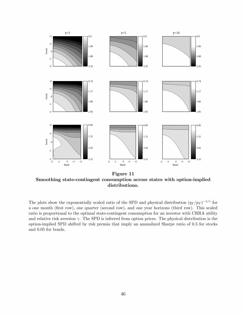
Stoc
k
γ=2
2
1
0
+1
+2
3.35
1.88
1.06
0.6γ=5
3.35
1.88
1.06
0.6γ=10
3.35
1.88
1.06
0.6
Stoc
k
2
1
0
+1
+2
2.95
1.86
1.17
0.74
2.95
1.86
1.17
0.74
2.95
1.86
1.17
0.74
Bond
Stoc
k
2 1 0 +1 +22
1
0
+1
+2
3.12
2.02
1.31
0.85
Bond2 1 0 +1 +2
3.12
2.02
1.31
0.85
Bond2 1 0 +1 +2
3.12
2.02
1.31
0.85
Figure 11Smoothing state-contingent consumption across states with option-implied
distributions.
The plots show the exponentially scaled ratio of the SPD and physical distribution (qT =pT )�1= fora one month (�rst row), one quarter (second row), and one year horizons (third row). This scaledratio is proportional to the optimal state-contingent consumption for an investor with CRRA utilityand relative risk aversion . The SPD is inferred from option prices. The physical distribution is theoption-implied SPD shifted by risk premia that imply an annualized Sharpe ratio of 0.5 for stocksand 0.05 for bonds.
46