Embed Size (px)
Citation preview

1
CONSUMPTION AND THE GREAT RECESSION:
AN ANALYSIS OF TRENDS, PERCEPTIONS, AND
DISTRIBUTIONAL EFFECTS
AN UPDATE USING REVISED NIPA DATA
Ivaylo Petev
(Stanford University and CREST)
Luigi Pistaferri
(Stanford University, NBER, CEPR, IZA and SIEPR)
and
Itay Saporta Eksten
(Stanford University)
Acknowledgments: We thank anonymous reviewers, Tullio Jappelli, Fabrizio Perri, and participants at the Recession Task Force Conference in Stanford, February 2010, for comments. This version has been updated to data available in August 2011.

2
1. Introduction
Consumption decisions are crucial determinants of business cycles and growth. As a
share of US gross domestic product (GDP) personal consumer expenditure has grown
steadily since the early 1970s to reach, by 2008, 70 percent of GDP. The particularity of
severe downturns is that consumer spending is likely not only to decline but also to
undermine the prospects for recovery. In this chapter we review the evidence on changes in
consumer spending during the so-called Great Recession which began officially in December
2007 and ended June 2009. The objective is to explore the distinctive consumption aspects of
this recession: How are the various components of household consumption affected? How is
the impact of the recession distributed across socio-demographic groups? How does the
recession compare to previous recessions? For the purposes of our analysis, we rely on the
most recent available national accounts data (August 2011) provided by the Bureau of
Economic Analysis (BEA), and micro-level data from the Consumer Expenditure Survey
(CEX) and the University of Michigan Surveys of Consumers.
There are three distinctive features of the Great Recession. First, it was deep.
Consumption per capita fell monotonically from the last quarter of 2007 (the official starting
date of the recession) throughout the first half of 2009 (a decline greater than 4 percent from
peak to trough). The decline was stronger for durables (and among them, vehicles), but
spending on nondurables and (especially) services also fell significantly compared to
previous recessions. Interestingly, consumption fell more (and it took more time to recover)
than disposable income, partly as a result of an increase in government transfers to
households (particularly, unemployment insurance claims). Second, the recession was long.
In fact, it was the longest recession to date since the Great Depression, with consumption still
trailing 2 percent below pre-recession levels after 15 quarters from the starting date and 8
quarters after the recession had officially ended. Finally, the varying impact the recession has

3
had across age, race, education and wealth groups resulted in a decline in consumption
inequality.
We single out four explanations for the observed change in consumption during the
Great Recession and for its unequal impact on socio-demographic groups. One is the “wealth
effect”, that is, the response of consumers to the destruction of wealth which followed from
the burst of the housing bubble and the stock market collapse of 2008. A second is an
increase in uncertainty, a decline in consumer confidence which may have reduced spending
through accumulation of precautionary savings (or reduction of debt) as well as deferment of
spending, most notably on durables. Third, changes in relative prices, especially gasoline,
may have reverberated on both the consumption of gasoline as well as of its complementary
goods like cars and transportation services. Finally, the credit crunch that followed the
financial crisis may have prevented some households from purchasing goods that are
typically acquired through borrowing, such as cars or other big-ticket items.
In the subsequent analysis, which is descriptive in nature, we provide suggestive
empirical evidence for each of these four factors, whose interaction and contribution to the
recession we leave for future research to disentangle with the benefit of more complete data
and a better vantage point. The paper proceeds with a discussion of the macroeconomic
picture (Section 2), followed by an analysis of trends in consumer confidence (Section 3), and
ends with a study of the redistributive effects of the recession using micro-level data on
consumer spending (Section 4); we conclude with a general summary of our results (Section
5).

4
2. The Macroeconomic Picture
In this section we review the evolution of personal consumption expenditure and
disposable income at the aggregate level. Unless noted otherwise, we use national income
and product accounts (NIPA) data provided by the BEA (as available in August 2011).
2.1. Personal Consumption and Personal Disposable Income
We start by asking whether trends in consumption spending during the Great
Recession are similar to trends in personal disposable income.2 Economic theory predicts that
the link between income shocks and consumption is strongest in the case of permanent or
unpredictable income shocks. Hence, consumption may fall as a direct consequence of a fall
in income induced by job loss, reduced hours or productivity, and negative returns from
assets, and more so if these are long-term changes to a household’s economic resources.
In Figure 1 we plot trends in per-capita personal consumption expenditure and
personal disposable income over the Great Recession period. Unless noted otherwise, all data
are expressed in per-capita terms, deflated using the CPI, and de-seasonalized.3 Both the
consumption and income series are set equal to 100 in the quarter immediately preceding the
start of the recession (2007:III). Remarkable about this graph is that while per-capita
consumption declines monotonically until the middle of 2009, disposable income first rises
and then, starting in 2008:III, falls precipitously (a 6 percentage point decline from peak to
trough). In fact, disposable income keeps falling for two quarters after the official end of the
recession.4 The breakdown of disposable income into its three components (transfers, wages,
and financial income) reveals that the fact that per-capita disposable income did not fall as
much as consumption fell during the recession is explained entirely by a strong increase in

5
government transfers to households (+18.6 percent from the last quarter of 2007 to the last
quarter of 2009), while both wages (-6.9 percent) and particularly financial income (-26.5
percent) fell as expected from the nature of the recession. The increase in government
transfers was partly attributable to an increase in the take-up rates of Unemployment
Insurance and Food Stamps,6 and partly to an increase in the generosity of means-tested
programs put forward by the Obama administration (extension of time limits for
unemployment insurance,7 tax cuts to households and businesses, and increase in food stamps
benefits and emergency TANF cash assistance, see Gary Burtless 2009).8
Figure 1: Consumption and Disposable Income
Of course, government transfers benefit primarily households on the lower end of the
income distribution under the assumption that the others can use accumulated savings to
insure themselves against income shocks. However, the sharp decline in financial income

6
during this recession has weakened the accumulated buffer-stock of wealthy households, who
in the absence of access to government transfers are likely to have lowered equally sharply
their consumption. As we shall see in the analysis of microeconomic data, this wealth effect
explains a considerable portion of the fall in consumption.
2.2. Total Consumption and Its Components
In Figure 2 we zoom out of the Great Recession period and look at the macro picture
for consumption components over the last decade. In particular, we plot the quarterly growth
of the three components of personal consumption expenditure (durables, nondurables, and
services) over the 2000-2011 period. The period includes two recessions, identified in the
graph by the shaded grey areas.
Three points are worth noting. First, the graph shows the well known fact that
spending on durables is much more volatile than spending on nondurables or services, with
wide upward and downward swings at the onset of booms and recessions, respectively.
Second, the last two recessions differ dramatically in terms of the impact on consumption.
The 2001 recession, induced by the deflating of the dot-com bubble and probably prolonged
by the 9/11 terrorist attacks, was very shallow. In fact, only durables declined in real terms
during this recession, and only by a negligible amount. Actually, in 2001 the growth in
overall consumer spending only slowed down relative to the previous years. The availability
of easy credit and the low unemployment rates are very likely to have provided the favorable
climate for the resilience during that recession of Americans’ consumer spending and for its
subsequent growth. In stark contrast to the 2001 recession, the Great Recession, which began
with the burst of the housing bubble and the global financial crisis that ensued, is

7
characterized by a decline in real terms in all consumption components. Throughout 2008,
the fall is substantial for expenditures on nondurables and precipitous for durables. While
consumption growth recovered in the second half of 2009, the recovery is likely due in no
small part to government intervention. The growth in spending on durable goods coincides
with the July-August government stimulus policy for car purchases, or “cash for clunkers”;
growth in spending on nondurables and services may be partly due to the effects of the
Obama stimulus (the American Recovery and Reinvestment Act of 2009, or ARRA), and
partly to rising consumer confidence (itself probably induced by the recovery in the stock
market).
Figure 2: Growth Rate of Consumption Components
Third, the Great Recession is substantially longer than its predecessor. In fact, it is one
of the longest on record. To put this in perspective and to appreciate the popular reference to
-8-6
-4-2
02
46
820
00q1
2001
q1
2002
q1
2003
q1
2004
q1
2005
q1
2006
q1
2007
q1
2008
q1
2009
q1
2010
q1
Nondurable goods Services
Durable goods Recession
Source: BEA, NIPA Tables 2.1, 2.3.4 and 2.3.5

8
this recession as the “Great Recession”, we plot in Figure 3 the Great Recession next to all
the US recessions that have occurred since the early 1970s. We first illustrate changes in
terms of quarterly growth rates of per-capita personal consumption expenditure (top left
graph) and repeat the comparison for the three main consumption components, durables (top
right), nondurables (bottom left), and services (bottom right). In each graph, consumption is
plotted over 15 quarters from the onset of the recession (normalized to be 100 in the quarter
immediately preceding the start of each recession). We also present the post-recession data in
a dashed pattern.9
Figure 3: Consumption During Recessions (Quarters From Start)
Since the early 1970s, the US economy has experienced six recessions: the 1973-75
recession (related to the 1973 oil shock, and remembered as the stagflation recession), the
1980 recession (induced by money supply restrictions), the 1982-83 recession (which resulted
from the combination of the energy crisis and the tight monetary policy of the Federal
951
001
051
101
15T
ota
l Con
sum
ptio
n
0 3 6 9 12 15
8010
012
01
40D
ura
ble
s
0 3 6 9 12 15
9510
01
0511
0N
ondu
rab
les
0 3 6 9 12 15
95
100
105
110
115
Ser
vice
s
0 3 6 9 12 15
Source: BEA, NIPA Tables 2.1, 2.3.4 and 2.3.5
The great recession vs. previous recessions
1973-75 1980 1982-83 1990-91
2001 Great recession

9
Reserve), the 1990-91 recession (the “Bush recession”, which resulted from the combination
of the 1990 oil price shock, the debt accumulation of the 1980s, new banking regulations and
a fall in consumer confidence), and the two most recent recession discussed above.
A number of facts emerge from looking at the top left panel of Figure 3. First, unlike
the 1980 or 1973-75 busts - when consumption fell quite dramatically right at the start of the
recession - during the Great Recession the fall in consumption has been initially more
muted.10 Second, a defining feature of the Great Recession is its much longer duration.
Moreover, consumption remains below the pre-recession levels for a longer period than any
other recessions represented in the graph. The historical comparison illustrates that an
economic bust is defined not only by the extent of the fall in the components of GDP (in this
respect, in the 1980 recession the US economy experienced a more dramatic 1-quarter fall in
consumer spending) but also by the time it takes to fully recover. For example, after 15
quarters from the onset of the Great Recession, consumption is still about 2 percent below
pre-recession levels. For comparison, the slowest-recovery recession (the 1990-91 one) was,
after 15 quarters from the onset, displaying a level of consumption almost 5 percent above the
pre-recession levels.
Trends in total consumption mask considerable heterogeneity in the behavior of its
three components. Spending on durables falls substantially, the fall in nondurable spending is
more moderate, while spending on services falls monotonically but at a substantially lower
rate. Interestingly, it is the rapid and significant recovery in services spending that helps the
recovery of total consumption in previous recessions (see the bottom right panel of Figure 3).
In the Great Recession, however, spending on services declines monotonically and fails to
recover altogether, which stands out as a further peculiar feature of this recessionary episode.

10
2.3. The Behavior of Durables, Nondurables and Services Components
A detailed look at the composite categories of durables, nondurables and services
spending reveals additional aspects of the Great Recession. For instance, breaking down
durable spending into its main components, Motor vehicles and parts, Furniture and
equipment, and Recreational goods and vehicles, we find that the bulk of the decline in per-
capita spending is attributable to purchases of cars (a 25 percent decline by the end of 2008)
and partly of furniture (a 10 percent decline), while spending on recreational goods (such as
LCD TV sets, iPhones, game consoles, and so on) is stable and even increases during the first
year of the recession (perhaps due to longer available free time resulting from job losses or
reduced working hours). All goods display some recovery in the second half of 2009, in
2010, and in the early 2011, although spending on cars remains substantially below pre-
recession levels.11 Part of the decline in durables may be explained by increased uncertainty
leading to the postponement of the purchase of goods with large adjustment costs and for
which the “cost of consumer remorse” is higher. In the case of cars, the higher price of its
main complementary good, gasoline, may underlie the decline in spending, evidence for
which we provide further below. Moreover, the financial crisis may have restricted available
credit lines for the purchase of durable and semi-durable products like cars and appliances.
Finally, there is evidence suggesting that consumer incentive programs were responsible for
the temporary increase in durable spending on vehicles in the second half of 2009. Note that
aggregate data do not allow us to make the distinction between extensive margins (how many
people buy the goods) and intensive margins (how much buyers spend on the goods that they
purchase) in order to disentangle the effect of the incentive programs from other confounding
factors; only the analysis of micro-level data permits this and such data is yet to be made
available (see the US Department of Transportation, 2009, for an analysis of the effectiveness

11
of the Consumer Assistance to Recycle and Save (CARS) program using customized
aggregate survey data).
We next break down nondurable spending into its main categories, Food at home,
Apparel, and Gasoline. The decline in spending on apparel continues well into 2009 (-8% at
the end of the recession) before going back to pre-recession levels as 2011 dawns, while food
expenditures recover slightly following a significant drop in the Summer and Fall of 200812
However, food spending for home consumption is still about 2% below pre-recession levels
15 quarters after the recession began (and food spending at restaurants etc. follows very
similar trends over this period). Gasoline consumption, on the other hand, appears to follow
closely the sharp oscillation of oil prices, which speaks to the contribution of change in
relative prices to amplifying the recession effect on nondurables spending. In particular, the
price of gasoline increased dramatically during the early stages of the recession (+50 percent
from the beginning of 2007 to the third quarter of 2008), went down very steeply in the last
few months of 2008, and then kept rising slowly for the rest of 2009, was stable for most of
2010, and it has been rising again lately. Hamilton (2009) attributes the rise in oil prices to a
bottleneck effect: a strong increase in demand at the international level not being met by a
proportional increase in supply. According to his analysis, the effect of rising oil prices
contributed to the recession by way of lowering demand for the popular but extremely fuel-
inefficient light trucks (SUVs). The claim is corroborated by the decline in the price of
vehicles for that same period, presumably reflecting a lower demand due to both lower
income and higher oil price. In conclusion, with the exception of the last quarter of 2008 and
the first quarter of 2009, spending on gasoline has fallen almost monotonically since the
recession began, and after 15 quarters it is still 12% below the pre-recession levels.
The unusual decline in food spending – a fundamental subsistence consumer category
and a solid indicator of living standards – raises concerns about the extent and depth of the

12
strain households are undergoing in the Great Recession. Note that earlier research by Aguiar
and Hurst (2005) shows that a decline in food spending is not necessarily associated with a
decline in nutritional content if consumers switch to home production or devote more time
shopping for better deals. Even though their research focused primarily on individuals who
face a sudden decrease in earnings and greater free time as they enter retirement, the logic of
the argument could be extended to individuals who expect involuntary job loss or reduced
work hours during the recession. Data from the American Time Use Survey (ATUS) allow us
to test whether in fact the decline in food spending corresponds to a parallel increase in time
spent on food preparation at home and on researching purchases.13 We find no clear evidence
in support of the hypothesis, most likely due to the fact that the increase in leisure came as a
shock to most individuals. Time spent on preparing food at home remains stable (about 30
minutes per day on average) both throughout the 2003-2008 period of available data and
particularly in 2008 when we observe food spending decline. We do record nonetheless a
minor fall in the amount spent shopping (from 24 to 22 minutes) and a very slight increase in
the amount of time spent on researching purchases (from an average of 0.06 in 2003-2007 to
0.10 minutes in 2008).
The last component of consumption that we study is services. The behavior of its sub-
aggregates (Transportation, Recreation, Housing and utilities, Finance and insurance, Food
services, and Health care) is very heterogeneous. Spending on health services increases14, is
stable for housing and utilities, but declines substantially for services related to transportation
(closely linked to swings in gasoline consumption and prices), with no recovery in sight (still
-15% after 15 quarters from the beginning of the recession) and recreation services (which
represent relative consumption luxuries), with a recovery in 2010 that comes to a halt in
2011. In regards to leisure and recreation services, our analysis of data from the ATUS shows
evidence of a recession-related substitution: we find a strong increase in time devoted to
13
home-based leisure activities (like watching TV and playing games) and a decline in social
activities requiring a money commitment (like hosting parties or going to sport or cultural
events). In sum, the overall stability of services masks declines in non-necessity spending that
are offset by spending on pre-commitments, difficult to change even during recessions, of
which rent and utilities are clear examples (see Chetty and Szeidl, 2006).
3. Great Recession: Great Uncertainty
In addition to concrete changes in the economic environment, recessions are
associated with a widening sense of uncertainty. Economic theory predicts that prudent
households will respond to increased uncertainty by delaying purchases of durable goods and
by saving for precautionary reasons (Bertola, Guiso and Pistaferri, 2004; Carroll and
Samwick, 2007).15 Recent research has also pointed to the effect that “uncertainty shocks”
may have on economic recessions (Bloom, 2009). Indeed, one possible reason for the decline
in consumption during recessions is the sense of increased insecurity about the future.
Individual perceptions about one’s prospects for employment, income, and human capital
investments acquire during recessions a societal dimension, the risk of which is to turn
perceptions into self-fulfilling prophecies and to exacerbate an economy’s downward plunge.
The uncertain prospects of the economy warrant thus a closer look at consumer confidence.
3.1. Consumer Confidence
We use consumer confidence data to explore the influence of uncertainty on consumer
behavior during the Great Recession. We measure consumer confidence with the University
of Michigan’s Index of Consumer Sentiment (ICS) (see Curtin, 2007). The ICS is a widely
used indicator, which is based on nationally representative surveys with a monthly sample of

14
at least 500 households, recruited on a rotating-panel basis. The index reflects responses to
five general questions about respondent’s perception of their current and future financial
situation, of current and future business conditions, and of favorability of conditions for
durable purchases.16 The index ranges from a minimum of 0 to a maximum of 200.17
Figure 4: Consumption Growth, Consumer Confidence, and Heterogeneity
One fundamental aspect of the consumer confidence data is that in the case of the U.S.
economy, growth in personal spending is trailed closely by consumer confidence as
illustrated by the historical trends in the top-left panel of Figure 4.18 During the “Great
Recession” the ICS declines dramatically. The depth of the decline is rivaled only by the low
levels of consumer confidence reached during the recessions of the mid-1970s and of 1980.
In other words, similar to its impact on actual consumption, the recession marks a complete

15
turnaround in consumer confidence after several decades of relative optimism, which peaked
in the late 1990s.
Noteworthy of the current dip in consumer confidence is its duration. Consumer
skepticism about the state of the economy lingered on for a year around exceptionally low
levels, between the second quarter of 2008 (ICS=60) and the first quarter of 2009 (ICS=58).
Slower than the increase in actual consumer spending, the recovery of confidence has been
compromised by another decline in the third quarter of 2010 (our last data point at the time of
writing).
Aggregate indices are likely to conceal potential differences in perceptions among
socio-demographic groups. In times of economic growth consumer confidence is predictably
lower among respondents who are poorer, older and of Hispanic or African-American origin.
But recessions tend to narrow between-group differences. The Great Recession is
unexceptional in this regard, if not but by the near-complete evaporation of between-group
differences in consumer confidence. By this measure, the Great Recession stands out along
with the recession of 1980 with its characteristic widespread feeling of uncertainty.
The gap between the reported confidence level of respondents from the bottom and of
respondents from the top income quartiles declined in almost every recession between 1978
and 2010 (the period for which data on socio-demographic variables are available in ICS).
The gap narrows due to the higher rate of decline in consumer confidence of high-income
respondents. As the top-right panel of Figure 4 shows, the decline is most abrupt for the Great
Recession, in which the confidence of respondents from the top income quartile lost fifty
points between the first quarter of 2007 and the last quarter of 2008. For comparison, the
level of consumer confidence for respondents from the bottom income quartile dropped by
approximately twenty points in the same period. The gap closed almost completely at the end

16
of 2008 when respondents from both the top and the bottom income quartiles reported
historically low confidence levels of fifty-nine and fifty-seven points respectively. Similarly,
as illustrated by the lower two panels of Figure 4, the dispersion in reported consumer
confidence across race or age groups isdeclines during the recession.
But if skepticism about economic prospects is widespread at the onset of recessions, it
develops unequally afterwards. Consider for instance the trend among respondents from the
top income quartile, whose consumer confidence decline in 2007 and 2008 is as sharp as its
relative recovery in 2009 and in the first half of 2010 (at the time of writing data are available
only until the second quarter of 2010). By contrast, the sense of uncertainty among
respondents from the bottom income quartile is more robust and the recovery of confidence
hesitant. The divergence in the trends of consumer confidence highlights differences in the
perception and, as this and the other chapters of the book amply document, in the concrete
experience of the recession by socio-demographic groups. The next subsection explores this
issue further as we look at the reasons respondents give to explain their perception and
experience of this last recession.
On a final note, it is worth noting the peculiar trend in consumer confidence among
Black respondents during the Great Recession. Their confidence level increased at a
remarkable rate compared to that of White and Hispanic respondents. The effect is robust to
differences in income, age and education. Its timing, from the second quarter of 2008
onwards, may reflect a complex mixture of economic concerns and of political hopes
associated with the last presidential election. This relative optimism resulting from the
apparent “Obama effect” overshadows, without necessarily improving, the concrete
economic consequences of the recession.

17
3.2. Perceptions of Personal Financial Perspectives
Behind the decline in consumer confidence there are concrete aspects of individuals’
financial situation deteriorating. Sixty percent of the individuals in our sample report that
their financial situation in 2009 is worse than in the previous year. For comparison, half that
number shared that opinion in 2006. In Figure 5 we stratify our sample by income (top and
bottom quartile), age (less than 30, 31 to 60, and older than 60), and race (White, Hispanics,
and African American). We plot the portion of each group that reports that their situation has
worsened (at the bottom of each panel) and, conditioning on reporting a worse financial
situation, we display statistics on the reasons respondents provide.
Figure 5: Perceptions of Worsening of Financial Situation
The answers illustrate people’s very tangible sense of the recession and its immediate
consequences: devaluation of financial assets, tight labor market, limited business
opportunities, and tough debt reimbursement. The mention of the pressure of higher prices
suggests a misunderstanding of the behavior of prices during the recession. With the
exception of the fluctuating gasoline prices noted earlier, most prices have changed only
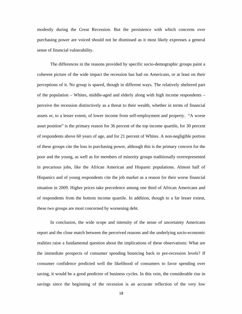
18
modestly during the Great Recession. But the persistence with which concerns over
purchasing power are voiced should not be dismissed as it most likely expresses a general
sense of financial vulnerability.
The differences in the reasons provided by specific socio-demographic groups paint a
coherent picture of the wide impact the recession has had on Americans, or at least on their
perceptions of it. No group is spared, though in different ways. The relatively sheltered part
of the population – Whites, middle-aged and elderly along with high income respondents –
perceive the recession distinctively as a threat to their wealth, whether in terms of financial
assets or, to a lesser extent, of lower income from self-employment and property. “A worse
asset position” is the primary reason for 36 percent of the top income quartile, for 30 percent
of respondents above 60 years of age, and for 21 percent of Whites. A non-negligible portion
of these groups cite the loss in purchasing power, although this is the primary concern for the
poor and the young, as well as for members of minority groups traditionally overrepresented
in precarious jobs, like the African American and Hispanic populations. Almost half of
Hispanics and of young respondents cite the job market as a reason for their worse financial
situation in 2009. Higher prices take precedence among one third of African Americans and
of respondents from the bottom income quartile. In addition, though to a far lesser extent,
these two groups are most concerned by worsening debt.
In conclusion, the wide scope and intensity of the sense of uncertainty Americans
report and the close match between the perceived reasons and the underlying socio-economic
realities raise a fundamental question about the implications of these observations: What are
the immediate prospects of consumer spending bouncing back to pre-recession levels? If
consumer confidence predicted well the likelihood of consumers to favor spending over
saving, it would be a good predictor of business cycles. In this vein, the considerable rise in
savings since the beginning of the recession is an accurate reflection of the very low

19
confidence of consumers. Their skepticism has lingered on in spite of the increase in
consumer spending in 2010. Whether this attitude expresses a long-lasting rather than a
temporary transformation of consumer behavior is open to speculation. It is worth noting that
consumer confidence is relatively inaccurate in predicting both the timing and the amplitude
of a business cycle because of the unequal effects of a recovery across socio-demographic
groups (Souleles, 2004), of which the data here provide ample evidence.
4. The Microeconomic Picture
Having shown in the preceding section evidence on differences in the perception of
the Great Recession, we now turn the attention on how actual consumer behavior varies
across socio-demographic groups. For this purpose, we use data from the Consumer
Expenditure Survey (CEX), which provides the only micro-level data available for the years
of the Great Recession (as we write, the data include monthly information up to February
2010).19 Given the complexity of the data, several technical explanations are in order before
moving to the discussion of our findings.
4.1. Consumer Expenditure Survey
The CEX, conducted by the Bureau of Labor Statistics (BLS), is used to help in the
construction of the CPI for certain items not covered by national income and product account
(NIPA). The survey contains a comprehensive measure of consumption, although research
has pointed out problems of comparability and coverage with NIPA (see Attanasio, Battistin
and Leicester, 2006). We refer the interested reader to the Appendix for more details on the
comparison between CEX and NIPA data. The subsequent analyses are based on the

20
comprehensive Interview sample of the survey, from which we extract data on households’
consumer expenditures, socio-demographic variables, and income and wealth information.20
In the analysis of the redistributive effects of the recession on consumption, we
compare annual growth rates of group-specific average consumption from 2007 to 2009.
Given that we condition on only a few demographic characteristics at a time, this analysis is
meant to be primarily descriptive. 22
The CEX reports household-level consumption. To control for differences in family
size, household expenditures are transformed into adult equivalents.23 Since our interest is in
consumption and not in spending per se, expenditures are deflated by the relevant price
deflator.24 To avoid attributing to the recession permanent differences in growth rates across
groups, we use 2003-06 (the last expansionary period) as a “control” period.
4.2. Redistributive Effects
Figure 6 summarizes the main results on the redistributive effects of the recession.
The first two panels on the top left stratify the sample by the age (30 or less, 31-64, 65 and
more) and education (high school or less, and some college or more) of the household head.
Middle-aged, high school or less and college educated individuals are the ones experiencing
the largest decline in consumption over the Great Recession (-3.9 to -4.4 percent). While this
is also the largest negative turnaround relative to the pre-recession period for the high school
or less group, for the college group the largest turnaround is for the young.. Older
individuals’ consumption is decreasing by 2.1 to 2.4 percent. Interestingly, when looking at
medians, the older group is the only group not experiencing any decrease in consumption, but
rather a slight increase.26 A simple life cycle model would predict that young, college-
educated households, who have low current income but high permanent income, finance their
consumption by borrowing against their future human capital. Since the recession was

21
characterized by an increase in the incidence of borrowing constraints, the consumption of
young, college-educated households may have declined as a consequence of the credit
restrictions they faced. Further, Wolff et al. (2010) predict that the fraction of homeowners
with negative home equity for 2009 is highest among individuals under 35 and those with
more than high-school education. Hence, consumption for young, college-educated
households may have declined also in response to this wealth shock. One reason that the
middle aged college educated group experienced a large negative growth in consumption is
that this group is holding a large share of the financial assets in the economy, making it more
vulnerable to the effect of wealth destruction which is well correlated with negative
consumption growth as we show below27.
In the top right panel of Figure 6 we stratify the sample by race. The largest decline (-
4.9 percent) as well as the largest drop in growth is associated with the Hispanic population
(The same finding holds true when looking at medians, -2.3 percent). What may explain these
differences?
We suggest two possible explanations. First, the difference observed between the
growth rates of the different groups may reflect occupation or industry composition effects.
As of 2008, for example, Hispanics accounted for 14 percent of total employment in the
economy but 24.6 percent of employment in the construction industry, which has been
severely hit by the recession. Indeed, unemployment rates grew more for the Hispanic
population between the second half of 2007 and the second half of 2008 (from 5.7 to 8.3
percent) compared to the white population (4.1 to 5.6 percent).29 Second, there may be an
association between negative home equity and negative consumption growth. As shown in
Table 1 in Wolff et al. (2010), Hispanics have a higher projected proportion of homeowners
with negative home equity (23.2 percent), compared to Whites (14.7 percent). Therefore, it is
possible that the decline in housing values induced by the burst of the housing bubble may

22
have pushed most sub-prime borrowers (who are over-represented among minorities, see
Calem, Gillen, and Wachter, 2004) into negative equity territory and hence induced a fall in
their consumption spending.
Figure 6: Means of Consumption Growth, By Groups
Next, we examine the impact of the recession on consumption by occupation,
distinguishing between private employees, public employees, and the self-employed. The
recession has an extremely negative effect (a 9.1 percent decline in total consumption) for the
self-employed, who in addition experience the largest change relative to the pre-recession
period. It is possible that reports of “self-employment” are masking effective unemployment,
and hence the decline in consumption captures the fall in income experienced by the

23
unemployed or under-employed (despite the role of the safety net). Given that the self-
employed have more volatile income than employees (public or private), it is possible that
this also reflects the effect of uncertainty, which suggests a more cautious consumer spending
attitude. Employees, private or public, have stable consumption patterns, although there is a
significant slowdown relative to the pre-recession period.
Lastly, the two bottom right graphs of Figure 6 stratify the sample by measures of
economic well-being, income (quintiles) and total assets (decile groups), respectively. The
measure of income is defined as total after-tax income from all sources including salaries,
income from business and farm, social security, unemployment benefits, workers’
compensation, welfare and food stamps, income from assets, pensions, rent, alimony and
child support. The measure of total assets represents the gross asset holdings of the household
including the household’s holdings in checking and saving accounts, bonds, securities, money
owed to the household and value of house and other real estate.30 Similarly to consumption,
we deflate and transform the assets and income variables into adult equivalent measures.
The middle bottom panel of Figure 6 shows that the fall in consumption is higher at
higher levels of income,31 even though differences across income group are not significant.
Moving on to the last panel of Figure 6, we look at consumption growth for three
groups: 1st to 5th decile of the wealth distribution, 6th to 9th decile, and those in the 10th decile.
This grouping is justified by the extremely high level of concentration of wealth; indeed,
individuals in the first five deciles have very little wealth, whereas those in the top decile own
about 50% of total wealth and 90% of financial wealth (total assets excluding housing) in our
sample.32 One remarkable finding is that respondents in the top decile of the wealth
distribution are the ones who decrease spending during the Great Recession (-7.5 percent).33
This finding holds also when looking at spending on nondurables and services, although the
negative growth rates are slightly smaller (-7.1 percent for the top wealth deciles). The fall is

24
smaller when looking at medians (-3.3 percent for total consumption and -3.9 percent for
nondurables plus services).34 The larger negative growth measured by means compared to
medians is the result of the consumption distribution becoming less skewed for the
households in the top decile of wealth.35
This finding may appear puzzling at first – indeed, wealthy individuals are expected
to have better tools to smooth their consumption during rough periods. However in the
context of the Great Recession, another effect might dominate the consumption behavior of
wealthy individuals. As shown in Wolff et al. (2010), the recession was characterized by
large wealth destruction suffered by rich individuals. This suggests that they lost a large
fraction of their “buffer” wealth, which was supposed to be used exactly for the purpose of
smoothing their consumption during the “rainy days” of the recession. To restore their
“buffer stock” these individuals may have needed to save more, which would decrease their
consumption growth.
The response of consumption to wealth shocks is known in the literature as the
“wealth effect” (see Poterba, 2000). Since shocks to wealth are presumably transitory, the
theory predicts that consumers should respond very little to them. The evidence on the actual
response of consumption to wealth shocks is mixed at best, but most papers do indeed find
small estimates. The evidence regarding the differential response to shocks to housing wealth
and shocks to corporate equity is also mixed.36 In what follows, we will not try to resolve this
debate, and instead take some representative lower and upper bound estimates of the wealth
effect from the literature.
A simple back-of-the-envelope calculation shows that the typical estimates of the
wealth effect for stocks found in the literature can explain a significant fraction of the decline
in consumption of the wealthy when one takes into account their initial high
wealth/consumption ratio. Table 1 details the calculation. For example, over the 2007-2009
25
period, households in the top decile of the wealth distribution lost on average about $209,000
of their assets (in 2007 dollars, corresponding to a 29 percent decline, see Panel A). Using the
window of estimates from the wealth effect literature (1 to 7 cents decline in consumption per
dollar of wealth destroyed), we predict that annualized consumption growth would have been
anything between -1.5 and -10.5 percent. The actual negative consumption growth
experienced by the wealthy was 7.3 percent, which shows that estimates of the wealth effect
might explain the actual decline in consumption experienced by the wealthy. Panel B repeats
the exercise for medians and confirms qualitatively these findings. We also find qualitatively
similar results if we consider a measure of wealth that excludes housing.
While individuals in the bottom part of the consumption distribution were less likely
to be affected by the wealth effect, another potential explanation for the bottom decile of the
wealth distribution showing moderate negative consumption growth during the Great
Recession is the large increase in transfer payments that took place during the recession.
Since transfer payments are more likely to be channeled to the poor, the increase in transfer
payments during this recession might have helped individuals with less wealth to smooth
consumption to a larger extent than individuals with more wealth. To address this point, we
compare inequality trends between the Great Recession and the 1990-1991 recession in
which there was a milder increase in transfer payments. We find that in the 1990-1991
recession, the top and bottom decile of the consumption distribution were moving together,
both showing large declines in consumption between the second half of 1989 and the first
half of 1991. While we cannot establish a causal relation between the increase in transfer
payments and the stability of consumption at the bottom decile of the wealth distribution in
the Great Recession, the findings from the comparison with the 1990-1991 recession appear
consistent with this idea.

26
4.3. Consumption Inequality and Consumption Mobility
As we have shown in the previous section, there is evidence that the consumption
distribution became less skewed to the right between 2007 and 2009. The direct implication
of this evidence is a decline in consumption inequality. In this section we take a closer look at
the consumption distribution and particularly at consumption inequality and consumption
mobility around the Great Recession. Heathcote, Perri and Violante (2010) document that
while disposable income inequality slightly increased in 2008 compared to 2007, inequality
in consumption of nondurable goods decreased. They show that this decline in inequality is
due to a large decline in the 90th percentile of nondurable consumption combined with a mild
decline at the 50th percentile and a slight increase at the 10th percentile. Our Figure 7 shows
the 10th, 50th and 90th percentiles as well as the variance of semiannual consumption
controlling for household size.37 The percentile series are normalized to 100 in the first half
of 2006. The figure shows that their findings hold also for our measure of total consumption
and that consumption inequality starts going back up during the second half of 2009 (right
after the end of the recession).
Two points are worth noting. First, changes in the variance of log consumption are
primarily driven by changes in the consumption of the 90th percentile, at least since 2007.
This finding is even more evident when looking at quarterly series (not reported here): the
correlation between the quarterly variance of log total consumption and the 90th percentile of
log total consumption is 0.8 while the correlation of the variance with the 10th percentile is
only -0.53. Therefore we can conclude that at least around the Great Recession, the decline in
consumption inequality is driven by decline in consumption in the upper parts of the
distribution. Second, in the period just before the recession the top and bottom deciles move
up at somewhat similar rates. However, during the recession, the top decile goes down
significantly, while the bottom decile remains relatively stable. The two trends, taken

27
together, imply a reduction in consumption inequality during the Great Recession. Once
more, this is in accordance with some of the group-specific trends in consumption growth
analyzed in section 4.2, namely the proportionally greater fall in consumption among the
wealthy (who are presumably also at the top of the consumption distribution) than among the
poor. Whether this is part of a more general trend, or an episodic event linked to the
recession, is hard to answer with our limited data, and hence we leave it to further inquiry
with better and more extended micro data.
Figure 7 : Consumption Inequality

28
Another aspect of redistribution one can look at is mobility. The distinction between
consumption inequality and consumption mobility is, effectively, a distinction between static
and dynamic features of a distribution. Inequality refers to the dispersion of consumption at a
point in time. Mobility describes movements within the consumption distribution over time.
A direct implication for welfare analysis is that stability in consumption inequality may mask
a great deal of mobility in the distribution.
The first step of our analysis is to construct an empirical transition matrix of
consumption. This requires panel data. The CEX is a quarterly rotating panel, and hence it
can be used to construct a measure of mobility. Our preferred measure is the Shorrocks’
index.38 This is an approximate measures of the fraction of individuals moving across the
distribution; a higher value of the index (which ranges from 0 to 1) is associated to a higher
degree of mobility from one year to the next. In Figure 8 we plot the monthly Shorrocks’
indexes as well as the local regression smoothed version (the solid line). Overall, there seems
to be a general declining trend in the amount of mobility in consumption. What can explain
this trend?
Jappelli and Pistaferri (2004) argue that under full consumption insurance (that is, in
an economic environment in which households can purchase insurance against all possible
shocks they face), individual consumption growth is independent of idiosyncratic shocks, and
it varies only in response to aggregate consumption growth. It follows that the cross-sectional
distribution of consumption of any group of households is constant over time. Of course
aggregate consumption can increase or decrease, so that the growth of consumption for any
household can be positive or negative, but the relative position of each household in the
cross-sectional distribution of consumption does not change over time. Hence, consumption
insurance implies absence of consumption mobility between any two time periods, regardless
of the nature of the individual income shocks and the time frame considered. While this

29
framework is clearly unrealistic in its pure formulation, the idea behind it is not. An
improvement in the amount and nature of insurance available to households (such as through
a process of financial market liberalization that makes credit more easily available and more
widespread as it happened during the 1990s and part of the 2000s) may well have contributed
to a reduction in the amount of mobility by attenuating the response of consumption to
shocks. The idea that credit market development in the US has helped households in
smoothing shocks more efficiently is also advanced by Krueger and Perri (2006).
Figure 8 : Consumption Mobility
An important question we may ask is whether the Great Recession reverts this
declining trend. The effect of the recession on consumption mobility may have worked
through the tightening of the credit markets. When credit is easily available, people can

30
smooth uninsurable shocks by borrowing and hence their consumption will not fluctuate
much from one year to the next. Hence, with well functioning credit markets there is less
scope for consumption mobility. The tightening of credit that occurred during the Great
Recession may have exposed more households to uninsurable shocks and hence increased
consumption mobility. To check whether the data support this view, we regress the Shorrocks
index on a linear time trend, a dummy for the period covered by the Great Recession
(December 2007-February 2009), and the interaction of the linear time trend with the Great
Recession dummy. We find that, as expected, there is a statistically significant general
downward trend in the data. The trend appears to have reverted or slowed down during the
Great Recession (the coefficient on the interaction is positive as the discussion above would
suggest); however, there are too few months covered by the recession to make this statement
unambiguously statistically precise.
5. Conclusions
In this chapter we have analyzed the behavior of consumption during the Great
Recession. There are three basic facts emerging from the analysis. First, the recession was
long. It set the record of being the longest recession since the Great Depression. Second, the
recession was deep. Consumption fell significantly in 2008 and in the first half of 2009,
before recovering slightly in the second half of 2009. However, the level of consumption in
the second quarter of 2011 was still about 2 percent below the pre-recession level. The fall in
consumption has been particularly strong among durables, but nondurables and service have
also fallen. Finally, we find important redistributive effects of the recession, in particular a
decline in consumption inequality and a slowing down in the decline in mobility that had
characterized the consumption distribution during the expansion years of the 2000s.

31
Our reading of the available evidence is that the Great Recession was not
consumption-driven. The fall in consumption occurred after the financial crisis and the
deflation of the housing bubble, not before. Of course, once the consumption decline was in
full swing, it contributed to prolong the recession. There is the broader and perhaps deeper
issue of whether the ultimate explanation for the financial crisis was an increase in the
demand for credit induced by an increase in consumer demand not matched by a concurrent
increase in permanent income. However, Mian and Sufi (2009) use US county data and
conclude that the subprime crisis was primarily driven by shifts in credit supply induced by
greater risk diversification (such as mortgage securitization) or simply greater assumption of
moral hazards on the part of lenders, rather than shifts in demand.
It is also interesting to notice the differences between the consumption response in the
Great Recession and the consumption response in the 2000-2001 recession. In the 2000-2001
recession consumption hardly fell – in fact, one can argue that the rapid recovery was due to
consumers keeping their spending high despite the recession. In hindsight, we know that the
high level of spending was sustained by unsustainable debt. In the Great Recession there is
instead ample evidence for household de-leveraging.
In the Introduction we mention a number of possible explanations for the behavior of
consumption during the recession. The first is the wealth effect. Given that the Great
Recession was characterized by large destruction of wealth, especially housing and equity,
this explanation is potentially important. We indeed find that the consumption of the wealthy
fell more than that of the less wealthy during the recession. Using the typical estimates of the
“wealth effect” available in the literature, we show that this factor can explain a significant
fraction of the fall in consumption experienced by the wealthy. This is not surprising. In
response to the large negative shock to their wealth, rich households may have responded by
increasing their savings in the attempt to restore their buffer stock. Nevertheless, the wealth

32
effect explanation is unlikely to make much headway in explaining the changes in
consumption of the less wealthy. It is possible, however, that the decline in housing values
may have pushed some “sub-prime borrowers” (who are over-represented among the
minorities) into negative equity territory and hence induced a decline in their consumption as
a result. A similar effect may have been at play among young, college educated households.
A second explanation for the peculiarity of the Great Recession that we advanced in
the Introduction was the increase in uncertainty. The financial breakdown of 2007 led to
historically low levels of confidence among Americans. Three years after the official start of
the recession and almost a year and a half after its official end, consumer confidence is yet to
recover to pre-recession levels. Furthermore, the steeper decline in confidence among high-
income households goes in line with our findings on the greater decline in the spending of
that group. On the other hand, the slower rate of recovery in the consumer confidence of
lower-income households reflects most likely not only their greater uncertainty but the
durable consequences that this recession has had on the stability and the future prospects of
their employment.
Third, there were significant concomitant price effects. The roller-coaster behavior of
the price of gasoline (and all complements to it) appears important enough to explain not only
the decline in the purchase of gasoline itself, but also of cars and transportation services.
These changes in relative prices may have had a large impact on poorer families’ budgets.
Finally, one of the main outcomes of the financial crisis was the credit crunch. Financial
intermediaries became extremely reluctant to lend, even to otherwise safe borrowers. This
may have prevented some consumers from purchasing big-ticket items that are traditionally
purchased on credit, such as cars and appliances.

33
Since the available data are still far from perfect, we believe it is still too early to
reach a definite consensus on the causes of the trends in consumer spending over the Great
Recession, and of its timing. We have attempted in this chapter to suggest possible
interpretations, present some suggestive evidence, and raise a number of important questions
that we leave for future explorations.

34
Appendix: CEX vs. NIPA
To justify our choice of using the CEX micro data when investigating the response of
personal consumption in the Great Recession, we first check to what extent population
estimates obtained using the CEX mirror aggregate data from the NIPA time series generated
by the BEA.39 In its officially distributed tables, the BLS provides only annual series of
aggregated CEX measures. Since we prefer to use quarterly and semiannual data to analyze
the effect of the recession, we construct these measures directly from the CEX micro data.
There are several issues which need to be addressed when mapping CEX to NIPA. First,
CEX consumer expenditures are collected by matching household expenditures to
classification codes (like food consumed at home, food consumed away from home, and so
forth). To be able to compare CEX aggregate measures to NIPA data, we need to take a stand
on how these classification codes are mapped into broader categories (such as food). We
adopt the NIPA categorization (as in Harris and Sabelhaus, 2000).40 Second, the CEX data
needs to be seasonally adjusted for comparability with NIPA series.41 Third, NIPA series are
available either in total or per-capita form. We obtain the per-capita equivalent in the CEX by
dividing average consumption across all consumer units by average family size. We find that
CEX quarterly nondurable consumption tracks the NIPA equivalent rather well – the series
have a 0.78 correlation since the year 2000. The equivalent series for total consumption
shows a lower correlation, 0.45. Both CEX series capture the decrease in consumption in the
Great Recession, though CEX total expenditure series is more volatile than the NIPA series.
The high correlation between CEX and NIPA consumption series, together with the finding
that the CEX captures the drop in consumption during the Great Recession, suggests that the
CEX is a suitable tool to use for assessing the consumption response in this recession.

35
References
Aguiar, Mark and Erik Hurst (2005), “Consumption vs. Expenditure”, Journal of Political
Economy, 113(5), 919-948.
Attanasio, Orazio, Eric Battistin and Andrew Leicester (2006), “From Micro to Macro, from
Poor to Rich: Consumption and Income in the UK and the US”, unpublished
manuscript.
Bertola, Guiso and Pistaferri (2005), “"Uncertainty and consumer durables adjustment”,
Review of Economic Studies 72(4), 973-1008.
Bloom (2009), “The impact of uncertainty shocks”, Econometrica.
Broda, Christian and Jonathan Parker (2008), “The Impact of the 2008 Tax Rebates on
Consumer Spending: Preliminary Evidence”, unpublished manuscript.
Burtless, Gary (2009), “The Social Protection for the Economic Crisis: The U.S.
Experience”, The Brookings Institution.
Calem, Paul, Kevin Gillen, and Susan Wachter (2004), “The Neighborhood Distribution of
Subprime Mortgage Lending.” Journal of Real Estate Finance and Economics, 29(4),
pp. 393-410.
Carroll, Christopher D., and Andrew A. Samwick (1997), “The Nature of Precautionary
Wealth,” Journal of Monetary Economics, 40(1), pp. 41—71,
Chetty, Raj and Adam Szeidl (2007), "Consumption Commitments and Risk Preferences”,
The Quarterly Journal of Economics, 122(2), pages 831-877.
Congressional Budget Office (2007), “Housing Wealth and Consumer Spending”.

36
Curtin, Richard (2007), “The University of Michigan’s Consumer Sentiment Index”,
Unpublished manuscript.
Hamilton, James D. (2009), “Causes and Consequences of the Oil Shock of 2007-08”,
Brookings Papers on Economic Activity, Spring 2009: 215-259.
Harris, Ed and John Sabelhaus (2000), “Consumer Expenditure Survey. Famnily level
extracts 1980:1-1998:2”, National Bureau of Economic Research, Unpublished
manuscript.
Heathcote , Jonathan, Fabrizio Perri and Gianluca Violante (2010), “Inequality in times of
crisis: Lessons from the past and a first look at the current recession”, VOX EU.
Kenworthy, Lane and Lindsay Owens (2010), “How Do Recessions Influence Public
Opinion?”, This volume.
Krueger, Dirk and Fabrizio Perri (2006), “Does Income Inequality Lead to Consumption
Inequality? Evidence and Theory” Review of Economic Studies Vol. 73(1), 163-93.
Ludvigson, Sidney (2004), “Consumer Confidence and Consumer Spending,” Journal of
Economic Perspectives, Spring 2004, 18(2): 29-50.
Mabli, James, Rhoda Cohen, Frank Potter, and Zhanyun Zhao (2010), “Hunger in Americas
2010”, Mathematica Policy Research.
Mian, Atif and Amir Sufi (2009), “The Consequences of Mortgage Credit Expansion:
Evidence from the U.S. Mortgage Default Crisis”, Quarterly Journal of Economics,
124(4), 1449-1496.
Parker, Jonathan A. & Annette Vissing-Jorgensen, 2009. "Who Bears Aggregate Fluctuations
and How?," American Economic Review, 99(2), pages 399-405, May.

37
Poterba, James M. 2000. “Stock Market Wealth and Consumption,” Journal of Economic
Perspectives 14, no. 2 (Spring), pp. 99-118.
Souleles, Nicholas (2004), “Expectations, Heterogeneous Forecast Errors, and Consumption:
Micro Evidence from the Michigan Consumer Sentiment Surveys”, Journal of Money,
Credit, and Banking, 36(1).
US Department of Transportation (2009), “Consumer Assistance to Recycle and Save Act of
2009”, Report to the House Committee on Energy and Commerce, the Senate
Committee on Commerce, Science, and Transportation and the House and Senate
Committees on Appropriations.
Wolff, Edward, Lindsay Owens, and Esra Burak (2010), “The Great Recession, Wealth
Destruction, and The Housing Market”, This volume.
Wolff Edward (2010), “Recent Trends in Household Wealth in the United States: Rising Debt
and the Middle-Class Squeeze”, Unpublished manuscript.

38
Table 1: The Wealth Effect for Top Decile of Financial Assets
Panel A: Weighted means (1) (2) (3) Estimate of the wealth effect from the literature 0.01 0.04 0.07 Average annual consumption 2009 59,528 Average annual consumption 2007 69,718 Average total wealth 2009 717,349 Average total wealth 2007 926,280 Predicted annualized consumption growth -1.50% -5.99% -10.49% Actual annualized consumption growth -7.30% Panel B: Medians (1) (2) (3) Estimate of the wealth effect from the literature 0.01 0.03 0.07 Median annual consumption 2009 48,814 Median annual consumption 2007 52,243 Median total wealth 2009 517,082 Median total wealth 2007 673,439 Predicted annualized consumption growth -1.49% -5.98% -10.48% Actual annualized consumption growth -3.30%

39
Endnotes
2 In the BEA definition, personal disposable income is the sum of “Compensation of employees, received” (wages and employers contribution to social security), “Proprietors' income with inventory valuation and capital consumption adjustments” (business income), “Rental income of persons with capital consumption adjustment” and “Personal income receipts on assets” (income from assets), “Personal current transfer receipts” (transfers from the government and businesses), net of taxes paid.
3 On average, durables account for about 10 percent of the total, nondurables for about 25 percent, and the remaining 65 percent is accounted for by services.
4 This comment is based on NIPA updated data as of August 2011. When we finished writing this paper for the “Great Recession” volume (April 2011), the NIPA data showed a much muted decline in disposable income (in fact, disposable income looked remarkably stable in these data). The updated data show a much deeper and longer recession in terms of the disposable income series. It is even possible that these new data will call into question the NBER dating of the recession.
6 The take-up rate is defined as the ratio of Beneficiary to Eligible Individuals (for Unemployment Insurance) or Households (for Food Stamps).
7 The remarkable extension of UI benefits to 99 weeks (from the conventional 26 weeks duration in most states) may have contributed to an increase in long-term unemployment rates by creating disincentives to search for active employment.
8 From the onset of the recession in 2007:IV to 2009:IV, spending on unemployment insurance soared by a staggering 303 percent. There was also a remarkable reduction in tax receipts (-29.4 percent) and an increase in veteran benefits (+21 percent) most likely associated with the impact of the Iraq and Afghanistan wars.
9 The line for the 1980 recession has a solid-dash-solid pattern because it overlaps with the 1982-83 recession.
10 The fact that consumption falls only late in the cycle suggests that it is not the engine of the economic bust. However, its late fall may also have contributed to the length of the bust itself. Note, however, that the attenuated response of consumption at the start of the recession could be explained by the effect of the 2008 tax rebate that families received in the first and second quarter of 2008. According to Broda and Parker (2008), consumption in the second and third quarter of 2008 was boosted by the receipt of the rebate, with most families spending it on food, mass-merchandise and drugs.
11 The reversal of the decline in spending on durables raises the question of whether the sharp decline in 2008 reflected tighter budgeting by consumers or simply a more cautious withdrawal from the market in the anticipation of impending lower prices. Indeed, by the first quarter of 2009, surveys were registering an upturn in consumers’ perceptions that the time was right for purchasing durable goods. Even though the richest Americans were particularly likely to find early 2009 a favorable time to make major purchases, when it comes to potential investments in a new home or vehicle, all income groups appeared more favorable toward making major purchases.
12 The usage of food stamps has also spiked up dramatically (see Mabli et al. (2010)).
13 ATUS is a time use survey conduced by the BLS, designed to measures how people allocate their available time to activities such as paid work, childcare, volunteering, and socializing.
14 Health spending has been growing almost monotonically since the early 1970s. In fact, growth rates slow down during the early 2000s and are basically flat during the Great Recession period.
15 There is indeed a strong increase in savings during the Great Recession. In fact, it was the first time in more than 25 years that savings increased on a consistent way for 2 years in a row. At the same time, there was a process of household de-leveraging. The debt-service ratio, having increased from 11 percent in 1993 to almost 14 percent at the outset of the Great Recession in 2007, fell to about 12.5 percent in just the following two years.

40
16 The five questions are : (1) "We are interested in how people are getting along financially these days. Would you say that you (and your family living there) are better off or worse off financially than you were a year ago?"; (2) "Now looking ahead--do you think that a year from now you (and your family living there) will be better off financially, or worse off, or just about the same as now?"; (3) "Now turning to business conditions in the country as a whole--do you think that during the next twelve months we'll have good times financially, or bad times, or what?"; (4) "Looking ahead, which would you say is more likely--that in the country as a whole we'll have continuous good times during the next five years or so, or that we will have periods of widespread unemployment or depression, or what?"; and (5) "About the big things people buy for their homes--such as furniture, a refrigerator, stove, television, and things like that. Generally speaking, do you think now is a good or bad time for people to buy major household items?" 17 The index’s computation involves the sum of the relative scores (X1, X2, X3, X4, X5) on each of the five question described in the previous note (i.e., percent of a favorable response minus percent of an unfavorable response, plus 100), divided by a 1966 base period total, plus a constant (which corrects for sample design changes from surveys in 1950s): ICS=2.0+(X1+X2+X3+X4+X5)/6.7558.
18 This is of course not a statement about causality. People’s lack of confidence may reflect information about the current state of the economy, rather than a predictor of future consumption behavior. Indeed, Ludvigson (2004) concludes that the forecasting power of consumer confidence indexes for consumer spending is at best very modest.
19 In the US, the only three general-purpose surveys with some information on consumption are the Health and Retirement Study (HRS), the Panel Study of Income Dynamics (PSID), and the Consumer Expenditure Survey (CEX). Unlike the CEX however, the HRS and the PSID surveys are conducted biannually and their last available waves refer to years prior to the current recession.
20 The CEX consists of two samples: a diary sample and an interview sample. The Diary is designed to obtain detailed expenditures data on small and frequently purchased items, recorded over the period of two consecutive weeks. The Interview sample surveys the whole range of expenditures of households for a maximum of five quarters. While expenditures are reported at every interview for the quarter preceding the month of the interview, income is reported only in the second and fifth interviews for a period of twelve months prior to the month of the interview. Information on assets is reported only in the fifth interview and refers to the amounts held as of the last month before the interview. In addition to stocks of wealth, households also report the change in wealth in the twelve months prior to the fifth interview, which allow researchers also to construct the initial wealth of the households at the time it enters the survey (namely, the stock of wealth just before the first interview).
22 The CEX sample for 2007 to 2009 consists of 270,487 monthly observations, corresponding to 27,876 households. We drop observations with incomplete income data, living in rural areas, observations for which consumption is reported for the month of the interview, individuals living in student housings, multiple household units, armed forces personnel and households with less than three reports per quarter (in this case we only drop the interview with the missing reports and not the entire household). The final sample consists of 188,958 monthly observations corresponding to 22,183 households. 23 The normalized measure is consumption/(# family members)0.5.
24 We deflate using the BLS all urban CPI. Since the BLS does not provide a deflator for the sum of nondurables and services, whenever this measure is used we use the services index to deflate this sum. This choice is driven by the much larger budget share of services (On average, services budget share is 70.6 percent while nondurables are 24.7 percent in the 2007-2009 sample).
26 Most of these patterns are replicated when examining other measures of consumption, such as nondurables or nondurables plus services, with the main difference being that for nondurables the most negative consumption growth (6 percent) is recorded for the young college educated group.
27 Middle aged college educated are 41.4 percent of our sample at 2007, but they are 58.4 percent of the individuals in the top financial assets decile for this year.
29 Source: Current Population Survey (CPS).

41
30 The allocation of individuals to income quintiles is done using the income data collected in the second and fifth interview. The allocation to asset deciles is done using the asset holdings data reported in the fifth interview. We therefore use only second in fifth interview, and only fifth interview observations of consumption when analyzing income and assets respectively. This implies that for income we are left with 91,091 observations for 2007 to 2009. For assets we are left with 46,055 observations for 2007 to 2009.
31 Parker and Vissing-Jorgensen (2009) report somewhat similar findings, showing that high-consumption households display larger responses to aggregate consumption shocks than households with low levels of initial consumption.
32 Wolff (2010) reports a somewhat similar number for financial wealth (81 percent) using data from the 2004 Survey of Consumer Finances, which is a much richer data set on the wealth of American households.
33 To obtain this figure, we compare average monthly consumption in 2007 for individuals who in that period were in the top 10% of the total asset distribution with average monthly consumption in 2008 for individuals who were in the top 10% of the total asset distribution in that period and repeat this exercise for 2008 and 2009. Ideally, one would like to have panel data and compare the consumption between the two periods of individuals who were in the top decile of the total asset distribution at baseline. Unfortunately, the structure of the CEX is such that this ideal comparison is not feasible. However, given that we have two observations on assets for most families, we have verified that there is very little mobility out of the top and bottom deciles of assets over a 12 months period.
34 We also calculated the growth of means and medians for financial wealth (total wealth excluding housing and real estate). When looking at means of total consumption, the 10th decile still shows the most negative consumption drop. When looking at medians, the 10th decile shows the least negative growth.
35 The ratio of consumption of the 90th percentile to the median consumption in the top wealth decile is 2.2 for 2007 and 1.96 in 2009.
36 For example, a survey by the Congressional Budget Office (2008) states that “a $1,000 increase in the price of a home this year will generate $20 to $70 of extra spending this year and in each subsequent year”, while Poterba (2000) writes that “the long-run impact of a $1 increase in stock market wealth is a consumption increase of 4.2 cents, while an increase in non-equity wealth raises consumer spending by 6.1 cents”. In contrast, Juster, Lupton, Smith, and Stafford (2005) report that their estimates “suggest that a one-dollar capital gain in corporate equities increases spending in a 5-year interval by as much as 19 cents” and that their analysis robustly shows that “the spending response to capital gains in corporate equities is larger than to capital gains in other assets, including housing”.
37 The definition of consumption is as in the previous section.
38 The index is defined as
q
i iipqq1
11 , where q is the number of quantiles in which the distribution has
been divided, and pii is the proportion of individuals who remain in quantile i between two successive periods. In our analysis, we work with deciles (q=10).
39 When comparing with NIPA, we use a less restrictive sample, dropping only observations for which consumption is reported for the month of interview. However, we also trim the top percentile of the distribution for each consumption category, to remove outlier.
40 We update the mapping to account for changes which have occurred in the CEX after 1998 – the last year for which they have constructed the mapping. 41 We perform the seasonal adjustment using the Census Bureau X-12-ARIMA software (note that for the micro data analysis the data is not seasonally adjusted).