Embed Size (px)
Citation preview

CONSUMPTION EXPENDITURE PATTERN OF'
SCHEDULED CASTE HOUSEHOLDS OF' KERALA: A STUDY OF IDUKKI DISTRICT
THESIS SUBMITTED TO THE
COCHIN UNIVERSITY OF SCIENCE AND TECHNOLOGY
FOR THE AWARD OF THE DEGREE OF
DOCTOR OF PHILOSOPHY
IN ECONOMICS
FACULTY OF SOCIAL SCIENCES
By
CELlNKUTTY MATHEW Reg.No.1552
UNDER THE SUPERVISION AND GUIDANC;:E OF
Dr. MARY JOSEPH T.
PROFESSOR
SCHOOL OF MANAGEMENT STUDIES ". "" ....
"-".
DEPARTMENT OF APPLIED ECONOMICS
COCHIN UNIVERSITY OF SCIENCE AND TECHNOLOGY
COCHIN. KERALA, INDIA
November 2003

SCHOOL OF MANAGEMENT STUDIES No: SMS ...................... .
COCHIN UNIVERSITY OF SCIENCE AND TECHNOLOGY KOCHI - 682 022
CERTIFICATE
Certified that the thesis "Consumption Expenditure Pattern of
Scheduled caste Households of Kerala : A study 0 f Idukki District 11 is the
record of bonafide research work carried out by Mrs. Celinkutty Mathew, under my
Supervision. The Thesis is worth submittingfor the degree of Doctor of Philosophy.
27-11- 2003 Cochin- 22
/f417" ;;;'$Y,">~'
Dr. Mary Joseph . Professor, School of Management Studies Cochin University of Science and Technology.
KOCHI- 682 022. KERALA. INDIA <l>: Office: 0484-575310. 575096,575946 Grams: Cusat, Kochi - 22. Telex: 885-5019. CU IN. Fax: 91-484-SnS95
e-mail: [email protected]

Vll
CONTENTS
CHAPTER I INTRODUCTION ................................................................................... 1 1.1 Consumption categories ....................................................................................... 2 1.2 Nature of Consumption ........................................................................................ 3 1.3 Factors affecting consumption options ................................................................ 3 1.4 Human Development in Kerala ........................................................................... 6 1.5 Statement of the problem ..................................................................................... 8 1.6 Significance and Relevance of the study ........................................................... 11
1.7 Objectives of the Study ...................................................................................... 12 1.8 Hypotheses ......................................................................................................... 13
1.9 Data and Sampling frame ................................................................................... 1 j
1.10 Methodology and Tools of Analysis .................................................................. 14 1.11 Relevance of selecting Idukki as sample area .................................................... 17 1.12 Profile of the study area ..................................................................................... 18 1.13 Idukki. District. .................................................................................................. 20 1.14 The Plan of the study ......................................................................................... 28
1.15 Limitations of the study ..................................................................................... 29
CHAPTER 11 REVIEW OF LITERATURE AND THEORETICAL FRAl\m WORK ...................................................... 33
2.1 Review of related studies ................................................................................... 33 2.2 General studies on consumption pattern ............................................................ 33 2.3 Studies on Consumption Pattern of Scheduled Castes ....................................... 46 2.4 Theoretical Background ..................................................................................... 52 2.5 Review of the Theory of Consumption Behaviour ............................................ 58 2.6 The Normal Income Hypothesis ........................................................................ 69 2.7 The Proportionality hypothesis .......................................................................... 70 2.8 The Rate of growth Hypothesis ......................................................................... 70
CHAPTER III CHANGING PATTERN OF CONSUMPTION EXPENDITURE IN INDIA AND KERALA ...................................... 80
3.1 Concepts and Definitions ................................................................................... 81 3.2 Distribution of persons by MPCE ....................................................................... 83 3.3 Average household size ..................................................................................... 85 3 .4 Average MPCE .................................................................................................. 86
3.5 Movement in Budget Share in Kerala ................................................................ 86 3.6 Movement in Budget share In India ................................................................... 90 3.7 Food Expenditure Pattern in Kerala ................................................................... 94 3.8 Food Expenditure Pattem in India ..................................................................... 95 3.9 Per capita consumption of individual items in India: Food items ...................... 97 3.10 Per capita consumption of individual items Kerala ......................................... 100 3.11 Per capita consumption of individual items in India ........................................ 103 3.12 Per capita consumption of individual items Kerala ......................................... 106 3.13 Consumption out of home- grown stock in India ............................................ 109

Vlll
3.14 Detailed Miscellaneous items: India ................................................................ 109 3.15 Detailed Miscellaneous item-Kerala ................................................................ 112
3.16 Educational & Medical Expenditure in India .................................................. 114
3.17 Education & Medical Expenditure Kerala ....................................................... 115
3.18 Consumption level and pattern of different fractile groups ............................. 116
3.19 Trends in average consumption expenditure and in consumption
pattern over the last two decades in India ........................................................ 120
3.20 Trends in average consumption expenditure and in
consumption pattern over the last three decades in Kerala .............................. 124
3.21 Possession of Durable goods ........................................................................... 125
3.22 Average Number of Durable goods possessed by households reporting possession ... 129
CHAPTER IV PROFII..E OF SClIEDULED CASTES ........................................... __ ......... 134
4.1 Introduction ...................................................................................................... 134
4.2 Caste system a general view ............................................................................ 134
4.3 Origin of Caste system and untouchability in India ......................................... 135
4.4 Caste system in Modem India .......................................................................... 138
4.5 The Period Since Independence ....................................................................... 141
4.6 Caste system in Kerala ..................................................................................... 145
4.7 Present Condition of Scheduled Castes in Kerala ............................................ 147
4.8 Economic Status .............................................................................................. 147 4.9 Occupational Status ofSC's ............................................................................ 150
4.10 Education ......................................................................................................... 152
4.11 Extent ofImmovable Property and Types of Houses ...................................... 154
4.12 Investment ........................................................................................................ 156
4.13 Household size ................................................................................................. 156
4.14 Food habits ....................................................................................................... 156
4.15 Use of modem garments, cosmetics and foot wear ......................................... 157
4.16 Special Programmes For Scheduled Castes in Kerala ..................................... 158
4.17 Summary .......................................................................................................... 159
CHAPTER. V CONSUMPTION PATTERN OF SCHEDULED
CASTES IN INDIA AND KERALA .•...............................•..•.•........... 163 5.1 Distribution of persons by MPCE .................................................................... l64
5.2 Average Household size of Scheduled Castes ................................................. 166
5.3 Average monthly per capita consumption expenditure .................................... 167
5.4 Proportion of Expenditure on Food ................................................................. 168
5.5 Proportion of Expenditure on Non - Food ...................................................... 169
5.6 Pattern of Consumer Expenditure of Scheduled Castes ................................... 171
5.7 Per capita expenditure ...................................................................................... 183
5.8 Percentage expenditure on food items to total food ......................................... 185 5.9 Movement in Budge share Kerala .................................................................... 187
5.11 Movement in Budget Share - All-India ........................................................... 190
5.12 Percentage Expenditure on food to total food expenditure
and items of non-food to total non-food expenditure in India ......................... 193

1X
5.13 Percentage Expenditure on food items to total food expenditure and items of non-food to total non-food expenditure in Kerala ................. : ..... 194
5.14 Expenditure on food ......................................................................................... 195 5.15 Change in Consumption pattern ....................................................................... 196
5.16 All India ........................................................................................................... 198
CHAPTER VI SOCIO ECONOMIC BACKGROUND AND CONSUMPTION PATTERN OF SAMPLE S-:HEDULED CASTE HOUSEHOLDS IN IDUKKI DISTRICT ........................... 205
6.1 Characteristics of Sample Households ............................................................. 205
6.2 Monthly per capita consumption expenditure .................................................. 217 6.3 Average Monthly Per capita Consumption Expenditure .................. ",,:, ? 1 ()
6.4 Per capita expenditure on different items of consumption: Engel ratio Analysis .................................................................. 222
6.5 Average Monthly Expenditure and Engel Ratios ............................................ 224 6.6 Percentage expenditure of each food item in total food
expenditure and percentage expenditure of each non -food item in total non-food expenditures ................................................................. 227
6.7 Engel ratio at the disaggregate level for comparable expenditure classes ....... 230 6.8 Elasticity of Consumption Expenditure ........................................................... 236 6.9 Factors that influence Consumption Pattern .................................................... 246
6.10 Monthly Per capita Consumption Expenditure among decile groups .............. 255 6.11 Sources of consumption ................................................................................... 261 6.12 Per capita Consumption of Individual Items food ......................................... :. 263
6.13 Per capita consumption of individual items: Non-food ................................... 273 6.14 Possession of Durable goods ........................................................................... 282
6.15 Goods for leisure time needs ............................................................................ 287 6.16 Average number possessed by households reporting possession .................... 291
CHAPTER VII FINDINGS AND RECOMMENDATIONS ...................................... 298 7.1 Distribution of MPCE among scheduled Castes .............................................. 298 7.2 Size distribution of Scheduled Castes .............................................................. 299 7.3 Proportion of Expenditure on food of SC's ..................................................... 299 7.4 Pattern of Consumption Expenditure of SC's .................................................. 300 7.5 Per capita Expenditure ..................................................................................... 300
7.6 Movement in budget Share .............................................................................. 30 I 7.7 Percentage expenditure ofSC's ....................................................................... 301
7.8 Per capita consumption expenditure ................................................................ 302 7.9 Rural Urban differences Kerala Consumption Pattern .................................... 302 7.10 MPCE among Occupation groups ................................................................... 302 7.11 Recommendations ............................................................................................ 306
BIBLIOGRAPHY ............................................................................................................ " 308
APPENDICES .............................................................................................................. i-xxxvii

x
LIST OF TABLES
Tabl. No. Title Page
1.1 Demographic indicators of sample area ........................................................................................ 27
1.2 Demographic indicators of Scheduled castes ................................................................................ 27
1.3 Demographic indicators of Scheduled castes in the study areas .................................................. 27 ... ~
3.1 MPCE classes ................................................................................................................................ 82
3.2 Per 1000 distributions of persons in the rural and urban sector .................................................... 84
3.3 Average household sizes in Rural and Urban areas ...................................................................... 85
3.4 Per Capita per month (30 days Expenditure (in Rs.O.OO) of broad groups of Food and non-Food items and % to total expenditure in rural areas of Kerala ....................................... 87
3.5 Per Capita per month (30 days Expenditure (in Rs.O.OO) of broad groups of Food and non-Food items and % to total expenditure in Urban areas of Kerala ................................... 88
3.6 Rural Urban differences in the value of per capita consumption of different groups of items in Kerala. based on 55th round ............................................................................ 89
3.7 Per Capita per month (30days) expenditure (in Rs. 0.00) of broad groups of Food and non-Food items and % to total expenditure in rural areas of all-lndia ................................... 91
3.8 Per Capita per month (30 days Expenditure (in Rs.O.OO) of broad groups of Food and non-Food items and % to total expenditure in Urban areas of All- India ................................. 92
3.9 Rural Urban differences in the value of pet" capita consumption of different groups of items in India ................................................................................................ 93
3.10 Percentage expenditure on different items of Food to total Food expenditure Kerala - Rural ................................................................................................... 94
3.11 Percentage expenditure on different items of Food to total Food expenditure Kerala - urban .................................................................................................. 95
3.12 Percentage expenditure on different items of Food to total Food expenditure India - Rural .............................................................................................. 96
3.13 Percentage expenditure C,il different items of Food to total Food expenditure, India - Urban ............................................................................................ 97
3.14 Per capita Quantity and value of cash purchase, consumption out of homegrown stock and total consumption of food items for a period of 30 days .......................................................... ix
3.15 Per capita quantity and value of cash purcr.ase, consumption out of homegrown stock and total consumption of food for a period of 30 days.
3.16 Edible oil (gm) consumed per person in 30 days ............................................................................ xi
3.17 Consumption of important Fruits & nuts ....................................................................................... 100
3.18 Monthly per capita quantity and value of consumption for Food items for Rural Kerala .............. 101
3.19 Quantity and value of per capita purchase and consumption over a 30-day period of important items of Food & Fuel for Kerala. Urban ................................................................... 102
3.20 Monthly Per capita quantity and value of consumption for non-food items by MPCE class for All India. Rural. ............................................................................................................... xiii
3.21 Monthly Per capita quantity and value of consumption for non-food items by MPCE class for All India. - Urban
3.22 Consumption of Pan, Bidis and Cigarettes. AlI- India ................................................................ xvi

Xl
3.23 Value (Rs.) of consumption of broad groups of non-Food items per person for a period of 30 days for each MPCE class for All India. Rural ............................... 1 05
3.24 Value (Rs.) of consumption of broad groups of non-Food items per person for a period of 30 days for each MPCCE class for All India urban ............................. 106
3.25 Monthly per capita of consumption for non-food items for Kerala rural ........................................ xix
3.26 Monthly per capita of consumption for Non-Food items for Kerala ................................................ xx
3.27 Value (Rs.) of consumption of broad groups of non-Food items per person for a period of 30 days for each MPCE class - rural Kerala ...................................... 107
3.28 Value (Rs.) of consumption of broad groups of non-Food items per person for a period of 30 days for each MPCE class - Kerala urban .................................... 1 08
3.29 Share of home produced component in tot~1 consumption selected items All-India Rural .......... 1 09
3.30 Monthly per Capita quantity and value of consumption for non-Food items by MPCE class for all India rural ........................................................................ 11 0
3.31 Monthly per Capita quantity and value of consumption for non-Food items by MPCE class for all India urban] ................................................................ 111
3.32 Monthly per capita quantity and value of consumption for non-Food items for Kerala- Rural ........................................................................................... 112
3.33 Monthly per capita quantity and value of consumption for Non-Food items for Kerala Urban ........................................................................................... 113
3.34 Monthly per Capita quantity and value.9f consumption for non-Food items by MPCE class for All India rural ....................................................................... 114
3.35 Monthly per Capita quantity and value of consumption for non-Food items by MPCE class for All India urban ..................................................................... 114
3.36 MonthYy per capita quantity and value of co~sumption for non-Food items for Kerala ...................................................................................................... 115
3.37 Monthly per capita quantity and value of consumption for Non-Food items for Kerala Urban ..... 116
3.38 Value (Rs) of consumption of broad groups of Food & non-Food items per person of 30 days for each fractile group. All-India ...................................................... 117
3.39 Value (Rs) of consumption of broad groups of Food & non-Food items per person of 30 days for each fractile group. All-India ..................................... 118
3.40 Value (Rs) of consumption of broad groups of Food & non-Food items per person of 30 days for each fractile group Kerala - Rural ............................ 119
3.41 Value (Rs) of consumption of broad groups of Food &
non-Food items per person of 30 days for each fractile group. Kerala - Urban .......................... 120
3.42 Value of consumption of broad groups of items per person for a period of 30 days by NSS rounds India Rural ...................................................................... 121
3.43 Value of consumption of broad groups of items per person for a period of 30 days by NSS rounds India ......................................................................................................................... 122
3.44 Percentage distribution of MPCE by 18 groups of consumption items in India .................. : ........ 123
3.45 Percentage distribution of MPCE over NSS rounds .................................................................... 124
3.46 Proportion of households possessing different items of Durable goods (Number per 1000) ................................................................................. 126
3.47 Average Number possessed per 1000 hou15eholds ..................................................................... 130

XlI
4.1 Percentage of SC households with income < Rs. 200 and size of households ........................... 149
4.2 Selected indicators of development for Scheduled Castes in Kerala .......................................... 152
4.3 Literacy level in Kerala and India ................................................................................................. 152
4.4 Percentage of literacy between different sub castes among SC's ............................................... 153
4.5 Percentage of persons who passed matriculation or above among SC's in Kerala .................... 154
4.6 Ownership of land and type of houses of Scheduled Castes ...................................................... 155
5.1 Percentage Population of SC below selected MPCE levels ........................................................ 164
5.2 Average household sizes of SC's ................................................................................................ 166
5.'3 Average MPCE for Scheduled Castes ......................................................................................... 167
5.4 Percentage of expenditure on food to total consumer expenditure for Scheduled Castes and General population ............................................................................ 168
5.5 Proportion of Expenditure on Non - Food Items to Total Consumer Expenditure for Rural and Urban Areas In Kerala & India .......................................... 170
5.6 Average consumer expenditure (Rs. 0.00) Per person for a period of 30 days for SC and General population and for the respective groups of households belonging to the monthly per capita expenditure class of 300 and above Rural.. ................................................................ 172
5.7 Average consumer expenditure (Rs. 0.00) Per - Person for a period of 30 days for Scheduled Castes and General population and for the respective groups of house holds belonging to monthly per capita expenditure class of Rs. 300/- and above urban ...................... 175
5.8 Per capita expenditure in (Rs) on broad groups of food and non-food items and % to total expenditure in Kerala for Scheduled Castes & General population ...................... 184
5.9 Percentage Expenditure on different items of food to total food expenditure for Scheduled Castes and C-.gneral population in Kerala .................................................................. 186
5.10 Per capita per month (30 days) expenditur~ in (Rs. 0.00) offood and non-food items and % to total expenditure for Scheduled Caste households in Kerala .............................................. 188
5.11 Per capita consumption (%) of different items in Kerala for Scheduled Castes
5.12 Per capita per months (30 days) expenditure in (Rs. 0.00) of food and ..................................... 189 non-food items and % to total expenditure for Scheduled Castes All India ................................. 191
5.13 Value (%) of per capita consumption of different groups of items in rural and urban India for Scheduled Castes ................................................................................ 192
5.14 Percentage expenditure on items of food to total expenditure and on items on non-food to total non-food expenditure in India .................................. : ..................... 193
5.15 Percentage Expenditure of Scheduled Castes on items of food to total food expenditure and items of non-food to total non-food expenditure in Kerala........... ............................................... 195
5.16 Expenditure on food in Total Consumer Expenditure [. %) .......................................................... 196
5.17 Average monthly per capita expenditure (Rs.) on broad groups of items in Kerala: Rural .......... 196
5.18 Average per capita expenditure (Rs) on selected broad groups of items urban Kerala .............. 197
5.19 Average per capita expenditure (Rs.) on st!lected items in Rural India ....................................... 198
5.20 Average per capita expenditure on selected broad groups of items in urban India ..................... 199
6.1 Sex wise Distribution of Sample Households .............................................................................. 206
6.2 Distribution of sample Se households into different sub- castes (%) ........................................... 207
6.3 Average household size in rural and urban areas ....................................................................... 207

Xlll
6.4 Size distribution of sample households ........................................................................................ 208
6.5 Age Structure of Sample Population. (%) .................................................................................... 209
6.6 Distribution of Person in the Sample Households Based on Education (%) ................................ 210
6.7 Distribution of persons based on occupation; number and percentage ....................................... 212
6.8 Distribution of sample households by monthly per capita income ............................................... 213
6.9 Income disposition between consumption and saving by income class -rural and Urban .......... 214
6.10 Type of structure of houses (%) ................................................................................................... 215 ., 6.11 General facilities available to sample households [% of households.] ......................................... 215
6.12 Outstanding Liabilities of sample hc~seholds .............................................................................. 216
6.13 -land ownership pattern of sample households ........................................................................... 216
6. i4 Distribution of sample population based on MPCE classes ......................................................... 218
6.15 Average MPCE and Average household size .............................................................................. 219
6.16 Distribution of sample households by expenditure on food and non-food items for various expenditure classes ........................................................................... 220
6.17 Average Monthly Expenditure per person on different items in the rural and urban areas ......................................................................................................... 223
6.18 Percentage Of MPCE on specific item groups: rural-urban differences Rural share>urban share ............................................................................................................. 226
6.19 Urban Share> Rural Share ......................................................................................................... 226
6.20 Results of 'F' test ...................................................... , .................................................................. 227
6.21 Percentage Expenditure on selected item& of food to total food expenditure .............................. 228
6.22 Percentage Expenditure on selected items of non-food to total non-food expenditures ......................................................................................................... 229
6.23 Average consumption (Rs.) and p~rcentage of broad groups of food and non-food items per person for a period of 30 days for each MPCE class of rural households ................... 231
6.24 Average consumption (Rs.) and percentage of broad groups of food and non-food items per person for a period of 30 Jays fOr each M?CE class of urban households ................. 232
6.25 Consumption pattern of rural households Estimated regression model: double log rural.. .......... 237
6.26 Consumption pattern of urban households Estimated regression model: double log urban ........ 238
6.27 Consumption pattern of rural households Estimated regression model: log inverse rural. .......... 242
6.28 Consumption pattern of urban households Estimatedregression model: log inverse urban ....... 244
6.29 Percentage of persons in different MPCE classes among different occupation types ................. 247
6.30 Percentage of persons in different MPCE classes among different occupation types ................. 248
6.31 Percentage Of persons in different MPCE classes among different Educational·types .............. 250
6.32 Income and expenditure on non-food items ................................................................................. 251
6.33 Education and expenditure on non-food items ............................................................................ 252
6.34 Occupation and expenditure on non-food items .......................................................................... 253
6.35 Rural urban Factor and expenditure on Non-food items .............................................................. 255
6.36 Percentage of consumption of broad groups of food and non-food items per person for a period of 30 days for each decile group - Rural... ............................................. 257

XIV
6.37 Percentage of consumption of broad groups of food and non-food items per person for a period of 30 days for each decile group - Urban ............................................... 258
6.38 Percentage Of consumption out of cash purchase, homegrown and gift loan in total consumption expenditure for rural and urban samples for different items ........................... 262
6.39 Distribution of sample households by monthly per capita consumption expenditure ................... 264
6.40 Monthly per capita expenditure on Cereals by households ......................................................... 265
6.41 Monthly per capita expenditure on Pulses by hQ~seholds ........................................................... 266
6.42 Monthly per capita expenditure on Milk & milk products by households ...................................... 267
6.43 Monthly per capita expenditure on Edible oil by households ....................................................... 267
6.44 Monthly per capita expenditure on Sugar by households ............................................................ 268
6.45 Monthly oer caoita exoenditure on Meat, fish & egg by households ............................................ 268
6.46 Monthly per capita consumption expenditure on Vegetables by households .............................. 269
6.47 Monthly per capita Consumption expenditure on Fruits & nuts by households ........................... 270
6.48 Monthly per capita expenditure on Beverages by households .................................................... 271
6.49 Monthly per capita expenditure on Spices by households .......................... " ............................... 271
6.50 Monthly per capita expenditure on Salt by households ............................................................... 272
6.51 Monthly per capita consumption expenditure on cooked food purchased ................................... 272
6.52 Monthly per capita consumption expenditure on Pan tobacco and intoxicants ........................... 274
6.53 Monthly per capita expenditure on Fuel & lights by households .................................................. 275
6.54 Monthly per capita expenditure on Clothing by households ........................................................ 275
6.55 Monthly per capita expenditure on Footwear by households ....................................................... 276
6.56 Monthly per capita expenditure on Education by households ...................................................... 277
6.57 Monthly per capita expenditure on Medical by households ......................................................... 278
6.58 Monthly per capita expenditure on Entertainment by households ............................................... 279
6.59 Monthly per capita expenditure on Goods for personal care by households ............................... 280
6.60 Monthly per capita expenditure on Travel by households ............................................................ 280
6.61 Monthly per capita consumption expenditure on Durable goods ................................................. 281 " 6.62 Percentage of households possessdlg different items of
Durable goods in rural and urban ................................................................................................ 283
6.63 Percentage of households possessing difff\rent items of Durable goods in each MPCE class - rural.. ............................................................................................. 284
6.64 Percentage of households possessing different items of Durable goods in each MPCE class- urban ............................................................................................... 285
6.65 Possession of Durable goods by MPCE classes Rural .................................... ; .......................... 291
6.66 Possession of Durable goods by MPCE classes-Urban .............................................................. 292

CHAPTER I
INTRODUCTION
The economic status of a society or community refers to its position as to
where it stands on the ladder of financial position. Most important determinants of
economic status of a society are its per capita income, the standard of living, the level
of consumption etc. Different indicators of the levels of living presents the "Macro"
as well as "Micro" level dimensions of the process of development. While per capita
income and per capita consumption expenditure are some of the macro level
indicators of development, the distribution of household expenditure is a micro level
indicator. The standard of living of a household can be understood from the
consumption pattern, and the quality of consumption budget clearly indicate the level
of welfare of the household. Food consumption pattern of household is an important
barometer of individual welfare and well-being in any country.
Human life is ultimately nourished and sustained by consumption. World
consumption has expanded at an unprecedented pace during the 20th century. The
benefit of this consumption has spread far and wide. More people are better fed and
housed than ever before. Living standards have risen. These achievements relate to
human development through consumption. Consumption clearly contributes to human
development when it enlarges the capabilities and enriches the lives of people without
adversely affecting the well-being of others)
But the iinks are often broken, and when they are, consumption patterns
and trends are inimical to human development. Today's cor(sumption is exacerbating
inequalities. And the dynamics of the consumption-poverty -inequality environment
nexus are accelerating. If the trend continues without change - not redistributing from
high income to low-income consumers, not shifting priority from consumption for
conspicuous display to meeting basic needs - today's problems of consumption and
human development will worsen.
Consumption must be (a.) shared: ensuring basic needs for all, (b)
strengthening: building human capabilities, (c) socially responsible: so the

2
consumption pf some does not compromIse the well being of others, and (d)
sustainable: without mortgaging the choices of future generations.
Abundance of consumption is no·crime. It has, in fact, been the lifeblood
of much human advance. The real issue is not consumption itself but its patterns and
effects. Consumption patterns to day must be changed to advance human
development tomorrow. Consumer choice must be turned into a reality for all.
1.1 Consumption categories
Consumption categories are formed mainly on the basis of the
commodities involved. Broadly speaking there are two categories: Food and non-food
consumption. Consumption to gratify hunger and thirst needs is food consumption2•
The consumption that is not related to the above but meant for satisfaction of health,
education, travel and recreational needs is regarded as non-food consumption.
However this categorization does not provide any idea about the essential and non
essential character of commodities in human consumption. We cannot say that non
food consumption meant for satisfying the needs such as clothing, shelter, health and
education is non-essential.
There is yet another classification purely based on the types of needs.
According to this classification we can distinguish between essential and non
essential consumption commodities. They are the categories of primary and
secon~ary consumption. Primary consumption involves the fulfillmeni of needs that
arise out of physiological bodily functions like thirst and hunger.3 These needs are
also called biogenic needs. Considering the basic nature, the needs for shelter
clothing, health and education can also be included in the category of 'primary
consumption, the secondary consumption comprises the gratification of a more
sophisticated structure of physiological needs which relate to social, cultural and
intellectual interests.4
Nevertheless, the above two categories remam inconclusive because
human needs are of varied nature and SUbjective to the individual consumer. This
inconclusive and SUbjective nature of needs creates constraints to form rigid and
3
exclusive categories of consumption. This conceptual fluctuation IS the major
limitation to studies pertaining to consumption.
1.2 Nature of Consumption
The dynamic nature of human needs gives consumption a dynamic I.
character. Human needs are always subjected to continuous change. The dynamic
character of consumption depends on the nature. of the society and ecollomy.
Variations in consumption are visible in different societies, as there exists a
difference in environmental, social, economic and cultural contexts. Human wants get
transfonned as the society grows and in turn cause substantial changes in the outlook
of the people towards consumption of commodities.
1.3 Factors affecting consumption options
Individual consumers are assumed to be in the best position to judge their
own needs and preferences and to make their own choices. It is fair to presume that
people know what they are seeking and have reasons for their preferences when they
opt for one consumption pattern over another.
Before being able to make any such decisions, however, the consumer
must at least be presented with choices. Yet millions of people face too narrow a
range of consumption options, which prevents them from enlarging their capabilities.
The existing distribution of consumption options points to serious shortfalls affecting
people in every society who rack access to a range of essential goods and services.
They may not be able to get enough food, may lack health care services or may have
little access to transport beyond their own feet. There are many factors causing these
constraints on consumption options. Income is not the only one. Other factors include
the availability and infrastructure of essential goods and services, time use,
infonnation, social barriers and the household setting.
1.3.1 Income
Income is an important means of widening the range of consumption
options, especially as economies around the world become increasingly monetized.

4
Income gives people the ability to buy diverse, nutritious foods instead of eating only
their own crops, to pay for motorized transport instead of walking, to pay for health
care and education for their families, to pay for water from a tap instead of walking
for many hours to collect it from a well.
The increasing deoendence of much consumption on private income
means that changes in income have a dominant influence on changes· in consumption.
When incomes rise steadily consumption rises for most of the population. But for the
same reason, when incomes decline, consumption also falls sharply, with devastating
consequences for human well being.
1.3.2 Availability and infrastructure of essential goods and services
Consumption options depend on the range of goods and services available -
from the market and state provisioning, from home production and common resources.
Many of the most basic essential goods and services-water, sanitation, education, health
care, transport and electricity-cannot be provided without an infrastructure.
Traditionally, these services have been provided first by the community
and then by the state. As markets develop and the technology improves, the services
increasingly are being provided by the private sector in areas where profit can be
made. Yet it is still the state that must ensure that, by whatever means, access is
available to all -rural as well as urban, poor as well as rich.
Even as markets increasingly take over services previously supplied by
the state, there is complementarity between public and private goods. Yet in many
countries and regions there is now a large and unhealthy imbalance, leading to great
social inequality. This was the forceful thesis presented by John Kenneth Galbraith in
his seminal work. The Affiuent Society' about 40 years ago.
1.3.3 Time use
Opportunities to consume can be severely limited by lack of time.
Women, spend many hours a day meeting the household's needs and have no time
left for education, better health care or community activities. Similarly, overworked
5
labourers may receive an adequate wage. but they often work long hours and are
denied the opportunity of regular leave.
1.3.4 Information
Information is the key to raising awareness of the range of consumption
options available and enabling the consumer to decide which choices are best.
Without information. there is no way of knowing what goods and services are
available in the market. and what services are being provided by the state and are. by
right, available to all. Advertising and public information campaigns play an
important role in this respect.
1.3.5 Social barriers
Income Cantot always remove barriers to access to opportunities. This is
particularly so when considerations of gender. class, caste or ethnicity limit people's
freedom to consume the goods and services they want. For example, people belonging
to certain ethnic groups might be denied equal access to education, employment and
other basic social services by the state, regardless of how much they earn.
1.3.6 The household- decision-making and upbringing
Much analysis of consumer decision-making assumes that the person
making the decision is the one who will directly benefit from the consumption. This is
far from the truth in many cases. A great deal of household consumption decision
making is in the hands of one person-often the mother or the father of the family.
Although this may lead to good outcomes, it can also be a source of inequity within the
family- Household values have a wider effect on the consumption options of individual
members. The education and upbringing given to children early in life play a critical
part in establishing their ability to make good use of the options available for living a
full and fulfilling life. The remarkable expansion and diversification in consumption
options have made it more difficult for consumers to make informed choices.
1.3.7 Globalisation and Consumption
As a result of increased purchasing pow~r and opportunity to purchase, a
change was manifest in the activity of consumption. The definition of what

6
constitutes a 'necessity' is changing, and the distinctions between luxuries and
necessities are blurring.5
Globalisation IS integrating not just trade, investment and financial
markets; it is also integrating consumer markets around the world and opening
opportunities. This has two effects --economic and social. Economic integration has
accelerated the opening of consumer markets with a constant flow of new products.
There is fierce competition to sell to consumers worldwide, with increasingly
aggressive advertising. On the social side local and national boundaries are breaking
down in the setting of social standards and aspirations in consumption.
As a consequence, a host of consumption options have been opened for
many consumers -but many are left out through lack of income. And pressures for
competitive spending mount. 'Keeping up with the Joneses' has shifted from striving to
match the consumption of a next door neighbor, to pursuing the life styles of the rich.
Some disturbing trends are observed. Pressures of competitive spending
and conspicuous consumption turn the affluence of some into the social exclusion of
many. When there is heavy social pressure to maintain high consumption standards
and society encourages competitive spending for conspicuous displays of wealth,
inequalities in consumption deepen poverty and social exclusion.
1.4 duman Development in Kerala
The development experience of Kerala has been umque and reflects
among several other things in its consumption patterns as well. It has received
worldwide acclaim for its unique features often hailed as the " Kerala model of
development". Admittedly, Kerala's development experience is unique in the sense
that a high level of quality of life co-exists with a relatively low per capita income.
This small state with a per capita income of about 160th of the per capita income of
the United States and an unemployment rate of about five times of that of the V.S has
achieved a level of development almost comparable to that the V.S in tenns of
achievements in health and education. Kerala, the southern most state in India, is . widely acclaimed for its unique pattern of social development. Significant progress

7
accomplished by the state in many spheres of social life, serves as a model to many
other societies. Education, health and demographic indicators are but a few examples
of the nature of social development in Kerala.6 No similar development has been
witnessed in any other Indian States so far. The state has several distinctive socio,
economic and demographic features. Very often Kerala is equated with other
developed countries.
The quality of life of people in Kerala is much above the average for the
country. Kerala is at the top in the country in human development. The Human
Development Index in Kerala [0.638] is much higher than the same for India [O.472f
Human Poverty has been estimated to reflect the level of deprivation. Kerala is far
ahead in the Human Poverty Index [19.9] of even the economically better off States.
The HPI for all India was 39.4.8 The prevalence of poverty in Kerala and India shows
that Kerala stood only next to Punjab and Haryana with 12.7% below poverty line
while for All -India 26.10 % were below poverty line.
Notwithstanding the enviable progress and unique features, Kerala
remains to be one of the poorer regions among the states in the Indian Union. With
regard to per capita income and its growth rate Kerala's position is below the national
level and that of many other Indian States. In terms of economic growth and
industrial production the state is still backward. Contrary to the lack of economic
growth, the living standards of the people of Kerala is comparatively high. What we
see in Kerala is a paradox, poor economic growth and high standard of living.
Consumption standard of its people is marked by a significant increase in the level of
consumption, of both food and non-food commodities. Compared to all India and
most of other states, people in Kerala allocate a considerable part of their income to
the consumption of non-food and non-essential items. But in developed economies,
such a trend was an outcome of industrialization. In those countries consequent upon
industrial growth, the purchasing power of the people increased tremendously. This in
turn improved both the level of consumption and the standard of living. Contrary to
this experience of developed economies, Kerala society manifests, the same kind of
consumption standards without any substantial produ~tion base.

8
1.5 Statement of the problem
The 20th centurie's growth in consumption, unprecedented in its scale and
diversity has been badly distributed, leaving a backlog of shortfall and gaping
inequalities. Consumption percapita has increased steadily in industrial countries
(about 2.3% annually) over the past 25 years,. spectacularly in East Asia (6.1 %) and at
a rising rate in South Asia (2.0%) Yet these developing regions are far from catching
up to levels of industrial countries, and consumption growth has Deen slow or
stagnant in others. The average African.households today consumes 20% less than it
did 25 years ago.
The poorest 20% of the world's people have been left out of the
consumption explosion. Well over a billion people are deprived of basic consumption
needs Inequality in consumption is stark. Globally, 20% of the world's people in the
highest -income countries account for 86% of total private consumption expenditure
the poorest 20% a minuscule 1.3%. More specifically the richest fifth Consume: 45%
of all meat and fish, and the poorest fifth 5, the richest 5th consume 58% of total
energy and poorest fifth less than 4%, the richest 5th have 74% of all telephone lines,
and the poorest fifth 1.5%, the richest 5th consume 84% of all paper, the poorest fifth
of 1.1%, The richest 5th own 87% of the world's vehicle fleet, the poorest fifth less
than 1 percent.
In India also the existence of large disparities in living standards between
regions and between classes of people is found. Wide economic disparities have been
observed between the rich and poor especially due to the low rate of economic change
among the poor section of the popUlation who generally fail to make use of the
development programme. The inequalities that persist between poor people and rich
women and men, rural and urban and among different ethnic groups are seldom
isolate, instead they are inter related and over lapping. Now economic growth and
industrial production has given rise to many serious problems. Widespread disparities
are being observed in the levels of living of different sections of the society. The
fruits of development have not been distributed equally among them.

9
All poor have not benefited equally from anti-poverty programmes.
Certain sections of society especially the scheduled Castes9 still suffer from
vulnerability. They are victims of illiteracy and rampant poverty. The policy of
protective discrimination was followed to reduce vast inequalities between the
Scheduled Caste and other strata of society. The out come of social and economic , "
refonns is uneven and far from satisfactory as far as achievement of the stated goals
is concerned
""
In spite of the various Constitutional safeguards and all the different
schemes for their upliftment the Socio economic condition of Scheduled Castes are
found to be much lower than that of the rest of the society. According to the 1991
census, 64% of Scheduled castes are agricultural labourers, who, without having land
possession, have to work as agriCUltural labourers for subsistence without any
security.iO And according to the Ninth Plan Draft Paper, the majority of Dalits (77%)
are absolute landless in India11 The Scheduled castes and Scheduled tribes constitute
near about one fourth of the population in India but control only 17.9% of the
agricultural land Around 87% of the Scheduled caste landholders belong to the
category of small and marginal farmers. 12 Less proportion of land ownership keeps
them in abject poverty, making them socially vulnerable
The condition of scheduled castes in Kerala has remained more or less
similar to that in other States in spite of the Kerala model of development. Special
provisions have been made for the socio-economic uplift of the Scheduled castes
communities in Kerala from time to time since the promulgation of the Constitution
of India. While the phase of progress of certain sections amongst Scheduled Castes is
encouraging, that of certain other sections among them is very poor
The commission on the socio-economic conditions of the scheduled castes
and scheduled Tribes in Kerala found that there are inter community and regional
imbalances even among the Scheduled Castes in the state.13 The findings of the survey
had brought to light the deplorable conditions of scheduled castes in Kerala. It showed
that the literacy among Scheduled castes was very much below the general level of
literacy. It was found that there are many hurdles for their children to peruse their
studies; the most important being the financial handicap. No appreciable change in their

10
occupation pattern was observed from that of the early times. They were found
associated with only humiliating, inferior, unclean work. A large percent of them were
either agricultural labourers or unskilled· workers except in the case of certain castes
which follow traditional occupation like cloth washing, basket making, and earthen
ware making on the whole it is seen that very few are able to separate their bond with
their age-old occupations and enter in to new areas of employment. The economic
status of the Scheduled castes were found to be very poor. As per the survey most of
the scheduled caste had no land of their own. Even in the case of those who owned their
own land, the extent in most cases is 10 cents or so.
Regarding the nature and type of houses occupied by scheduled castes it
was seen that less than 10% live in pucca houses. The schemes for giving grants and
loans for the construction of the houses for them have not found made any
appreciable impact on their environmental and living conditions.
The level of income of the Scheduled castes was found very poor. These
households were engaged in low paying occupations and most of them do not get
sufficient income for their subsistence. The socio economic survey showed that a large
% of the households are getting Rs. 200 or less per month. The condition of th~
majority of the households is deplorable as revealed by the survey. A monthly income
of Rs.200 or less means a per capita income of Rs. 40 or less as the average household
size was more than five. Households below poverty line were found to be 50% in most
of the Scheduled castes as per the report. Regarding investment the survey also found
that no household or less than 5% have bank deposits. Majority of them being below
the poverty line cannot naturally think of nothing but mere survival.
The survey also ascertained the items consumed by each household
during one month. The items used by all the households are Cereals, Spices and Salt.
Nutritious items like Egg, Milk, Ghee and other luxurious item are not found popular
with these households. Even if they are having cattle or poultry the products were to
be exchanged for other cheap varieties of food like Tapioca or other Tubers.14 Their
low-income levels compels them to remain in the low level of living.

11
In Kerala Scheduled Castes constitute 9.6 % of the total population while
the % of agricultural land 15 they owned is 2.80%. Their average landholding was only
0.07 percent, which was significantly worse than the National average, with only the
Punjabi Scheduled castes being behind in share of land holding. The national average
of 0.49 hectares for Scheduled castes was significantly lower than that of the general
population. 16
Overall, monthly expenditure of Scheduled castes in Kerala was found
about three-fourth of that of general population and this had fallen to 68.2 per cent for
urban Scheduled castes in '87-88. Statistics on employment and unemployment
showed that Kerala Scheduled Castes still suffer disproportionately.
Selected indicators of development for Scheduled castes show that the
percentage of population below poverty line among them is much larger (36.43%) as
compared to the general category of households (25.76) in Kerala. 17 Among them a
large section of population continues to be out side the reach of development
programs in spite of all the different schemes introduced for their upliftment. A
successful implementation of the strategies of development for Scheduled castes in
the last five decades would have by now reduced the socio, economic differentiates to
a nearly zero level, but the reality is different. The trickle down theory has failed to
raise the living standard ofthe poor and vulnerable section.
The economic disability imposed by poor asset possession and a host of
socio-cultural features have rendered their participation in the development process
less than average. The low-income level of Scheduled Castes compels them to remain
in the low level ofliving. The findings of the report showed that the living conditions
of the Scheduled caste s were very deplorable in the state as compared to that of the
General population and 'Kerala model of development' had not made any appreciable
impact on their lives.
1.6 Significance and Relevance of the study
Today Scheduled Castes are somewhat an enlightened lot but social . inequalities still exist. A slow pace of reforms is taking place for improving their
12
condition though much work remains to be done to put them back into the
mainstream society, and make them politically, socially and economically equal.
There is a scarcity of good publication on the state of the Scheduled castes. Truly they
have been marginalized as objects of our country rather than being treated as its
subjects. Inspite of forming a large proportion of the population they have just been
receiving minor reference in earlier studies.
There are not many studies of the consumption levels of Scheduled Castes
at the macro level. This is because the National sample Survey organization, which is
the only official agency that collects such data for the whole country, does not
generally publish date separately for Scheduled castes.18
The Scheduled castes have been studied as Socio-economic group by
several researchers such as Singh (1982) Joshi (1981), Subramanian and Deaton
(1991).19 They were mainly concerned with sociological and political aSpects. Micro
level studies with a focus on economic aspects have been under taken by Sundari
(1981), Saradamoni, Nayak (1984),20 Bhattacharya (1986) and Sagar (1994).21 Most
of these studies are based on secondary data, like the Census, Reports of the
Commission for SC/ST (1982).22 Most of the few economic studies on the Scheduled
caste concentrate on their educational and occupational structure and deal with its
effects on their welfare.
While studies abound on the consumption expenditure among rural and
urban households for various expenditure classes, little effort has been made to study
the consumption expenditure pattern for Scheduled Castes in rural and urban sectors.
The present study on the consumption pattern of these households in Kerala is an
effort to collect research and evidence on their present conditions.
1.7 Objectives of the Study
a) To examine consumption pattern among the SC population.
b) To examine the differences in the average consumption expenditure of
different decile groups of sample SC population.

13
c) To examine the consumption expenditure elasticity of items m the
consumption basket of se households.
d) To analyze the variations in expenditure of se households on food, non-food
and total expenditure.
e) To examine the association b~tween consumption expenditure and variables
such as income, education, occupation and area of residence.
1.8 Hypotheses
4) TI,Ci"C i~ ~i&,ifiCciiiL Jifference in the consumption elasticity of different items
among se households.
b) There is a significant difference in the average consumption expenditure of
different decile groups.
c) There is significant association between consumption expenditure and income,
education, occupation and area of residence.
1.9 Data and Sampling frame
A multi stage sampling procedure was adopted for selecting the sample
units. Scheduled castes constitute 9.92 percent of the popUlation of kerala While
10.98 percent of the rural population are se's only 6. 96 percent in urban areas are
SC's. In 6 districts of kerala viz., Idukki, Kollam, Palaghat, Pathanamthitta, Trichur
and Trivandrum the percentage of se population is higher than that of the state
average From these districts Idukki district was selected at random asing lottery
method to study the consumption pattern of se households. The district was divided
into rural and urban areas with Panchayats constituting the rural areas and
Municipalities constituting the urban areas. Panchayats with se popUlation greater
than 10% were identified. From among them one Panchayat was selected at random.
There being only one municipality in the district, that was selected for the study. In
the selected panchayat and municipality, 5 wards each with the highest percentage of
SC popUlation were selected at random. Sample of 100 households were selected at
random from the selected wards in both the Panchayat and Municipality, in
proportion to the se popUlation in each ward. Thus pnmary data were collected from
a total of two hundred households.

14
1.10 Methodology and Tools of Analysis
The present study of consumption expenditure pattern of scheduled castes
in Kerala investigates the following aspects. (1) The consumption pattern among the
Sc population (2) The average consumption expenditure of different decile groups of
sample Sc population (3) The consumption expenditure elasticity of items in the
consumption basket of Scheduled castes (4) The differences in the expenditure of
Sc's between food, non-food and total expenditure (5) The association between
consumption expenditure and variables such as income. education. occupation and
area of residence.
1.10.1 To examine the consumption pattern among Sc population
Exanlination of consumption pattern among Scheduled caste population is
done by analysing distribution of population by Monthly Percapita Consumption
Expenditure, the movement in budget shares on each item of expenditure, distribution
of total MPCE for food and non-food, rural urban differences in MPCE, consumption
out of different sources namely purchases, home grown stock and gift or loan,
changes in value of consumption, possession of durable goods among different
MPCE classes, trends in average consumption expenditure and consumption pattern
based on NSSO data for the period 1983-1993-94. Using primary data collected from
200 sample households. This was done separately for rural and urban samples.
1.10.2To examine the average consumption expenditure of different decile
groups of sample population.
Differences in consumption pattern of poorer and richer segments of
popUlation ranked by MPCE has been attempted by using appropriate deciles of the
MPCE distribution of class limits. Separate sets of consumption estimates for
different decile groups of sample popUlation are presented. Thus differences in the
consumption pattern of poorer and richer segments of the sample popUlation (ranked
by MPCE) is studied by examining the differences in their average MPCE on each
item of expenditure namely food and non-food. This includes the average MPCE for . 10 decile groups or classes ofMPCE starting from bottom 10 percent and ending with

15
the top 10%. Graphical representation of consumption pattern of lowest and highest
spending brackets is provided. Consumption pattern of the different decile- groups are
further studied by estimating proportion of expenditure on food and non-food items
and comparing the results. This is done separately for rural and urban sectors.
1.10.3 To examine the consumption expenditure ehsticity of items in the
consumption basket of Sc households.
Consumption expenditure elasticity of each food and non-food items in
the consumption basket of Sc Households is examined by using the Engel elasticity
expenditure separately for the rural and urban sample. A detailed explanation of the
Engel theory and the theoretical background of the present study are presented in the
section 2.4 of chapter ll. For the estimation of expenditure elasticity, four functional
forms have been selected namely, linear, double log, log inverse, and log-log inverse ~
functions.
a.
b.
c.
d.
Double log: logEij = a + ~logEj + U j
Log Inverse: logEij = a + p{If Ej)+ U j
1 Log-log Inverse: log E ij = a + P log E j + r - + U j
Ej
Where Eij is the MPCE of the ith item by /h household Ej is the total
monthly per capita expenditure of jth household. «, ~ and y shows parameters to be
estimated and u is the random disturbance term.
1.10.4To analyse the vari&tions in expenditure of Sc households on food, non
food and total expenditure.
Examination of the relative shares of expenditures on each food and each
non-food items among Schedule Caste households has been done by estimating Engel
ratios based on primary data for rural and urban sample in general and also separately
for different MPCE classes. First Engel ratios for each item of expenditure to total
expenditure has beWated for each item of food and non- food for rural and

16
urban sample separately. Then sample households have been grouped into 5
comparable expenditure classes. Engel ratio for each item of food, and non-food is
estimated for each expenditure class. Further an 'F' test was carried out for finding
out rural urban variation in the distribution of MPCE for food, non-food and total
expenditure separately for the sample households.
1.10.5 To examine the association between consumption expenditure and
variables such as income, education, occupation and area of residence.
Examination of the differences in the expenditure on non-food items
among SC households belonging to different income levels, education levels,
occupation categories and geographical regions has been done by finding out the
association between Monthly Percapita Consumption Expenditure and each of those
variables using 'i' test. As per the results of the 'F test rural-urban differences were
~~~~b~~~~~b~~~~~b
total expenditure. Hence association of MPCE to various detenninants has been
estimated by taking expenditure only on non-food items
For estimating association of income and expenditure on non-food items
Scheduled caste households are classified in to three per capita income classes: lower
class (Rs.1-400), Middle class (Rs.400-600), and upper class (Rs.>600). Besides
sample households have been grouped into two per capita expenditure classes on the
basis of expenditure on non-food items. The classes are Rs.1-200 and > Rs 200. X2 test
was carried out to find association
For finding out the association between educational standard of the head
of the household and expenditure on non-food, SC households are classified in to 3
groups on the basis of education of the head of the household namely, below. Std V,
Std V - Std X, and >Std X. Similarly per capita expenditure on non-food was
classified in to four categories, Rs.I-IOO, Rs.100-200, Rs.200-300 and >Rs.300. X2
test was applied to find association
For finding out association between non-~ood expenditure and occupation
sample households are grouped into seven occupation classes in rural and urban
17
sectors. The % of households in each occupation category showed that a larger % of
se households fall in certain categories such as 'other labourers' and 'agricultural
labourers' s in both rural and urban areas and the % in the other categories such as
'fanners', 'self-employed' and 'employed' were found comparatively much lesser.
Hence for the purpose of finding the association between occupation level and
expenditure on non-food items households of certain occupation categories with
lower % of households in the sample are being clubbed together with the adjacent
class. Thus the sample Scheduled caste households are classified in to 3 occupation
categories on the basis of occupation of the head of the household: agricultural labour
households, other labour households and salaried class households. Also the 200
sample households have been grouped into 4 per capita expenditure classes on the
basis of expenditure on non-food items. The classes are Rs.l-100, Rs 100-200,
Rs200-300 and >Rs 300. X2 test was applied to find association between occupation
and expenditure on non-food items.
To find the association between place of residence factor and per capita
expenditure on non-food t he Sample scheduled caste households have been classified
in to two categories based on their place of residence namely, rural and urban. The
200 sample households have been grouped into 4 per capita expenditure classes on
the basis of expenditure on non-food items. The classes are Rs.I-I00, Rs 100-200,
Rs200-300 and >Rs 300. X2test was applied to find association between place of
residence and expenditure on non-food items.
Per capita Expenditure on each food and non-food item has been studied
for identifying necessary and luxury items in their consumption baskets. Possession
of durable goods by scheduled caste households has been analysed to study the
tendency of luxuries consumption among Scheduled castes.
1.11 Relevance of selecting Idukki as sample area.
As per census of India 2001 Scheduled castes constitute 9.91 % of total
popUlation of Kerala. The Rural Urban distribution of Scheduled castes in Kerala
shows that in all the districts the great majority of. Scheduled castes live in rural

18
areas.23 Of the total Scheduled caste population in the State 81.48% live in rural areas
and only 18.52% live in urban areas.
Idukki district was chosen, as the area of study. Among the districts in
Kerala Idukki district has the highest % of scheduled castes living in rural areas
[namely 98%]. The distribution of Scheduled castes in the district is the most typical
in comparison to that in the State. In Kerala while 11 % of rural population are ..
Scheduled castes; only 6.90% of popUlation in urban areas is Scheduled castes. The
proportion of Scheduled castes in total rural population is 14.98% and in urban areas
6.02 % in the district. Idukki is one among six districts in Kerala where the % of
Scheduled castes is above the State average.
As per 2001 census the literacy rate of the District is 88.58 % with a male
literacy of 92% and f~e literacy of 85%. Female ~~y of Idukki District is very
backward as compared to other districts. The literacy rate for Scheduled castes in the
districts is only 74%. While the same for Scheduled castes in the State as a whole is 82.4%.
In the State among Scheduled castes 41.21% are workers and 58.79 non
workers. The % distribution of Scheduled caste popUlation into main workers, marginal
workers and non - workers in the different districts show that Idukki has the highest
percentage [47.55%] of workers among Scheduled castes which is greater than the
corresponding State average [41.21%]. In the district among Scheduled castes majority
of workers belong to plantation works namely cardamom and tea plantations works.
While the % of males in total workers in Idukki district is 53.51, that of females 41.57.
For the State as a whole the corresponding figures are 50.96 and 31.73 respectively.
The male and female work participation is the highest in the district among Scheduled
castes in the State.24 Hence Idukki district was selected to study the socio-economics
status of Scheduled caste communities and their consumption pattern.
1.12 Profile of the study area
The forgoing analysis of secondary data in chapter IV, V has revealed that
the Scheduled castes in India have a much lower income and hence lower
consumption standards than the rest of the society.

19
The economic development of a region is conditioned by the economic
and non-economic .factors; the importance of latter has considerably increased in
recent years. The attitude, motivations and composition of the community pay a . predominant role in shaping the economic development of a region. Naturally,
households with in a region differ in many respects, in location, in size, in
occlopational structure, in the average income, savings and livi~g standards. All these
characteristics economic, social and demographic in the aggregate, explain the
differences among the various households. An extensive an~lySis to identify the
relative impOrL81iCe uf the f~tul:' UCtC;l111il~l1l:. L11C lcv~l!; of income and consumption
pattern has to deal with factors such as family composition, Education, age structure,
occupational structure of the households etc. In other words the relation between
income and consumption changes significantly from one household to another due to
the interaction of these factors
The consumption pattern of general households in India and Kerala has
been discussed using the available secondary data from different sources in chapter
ill for rural and urban areas. Chapter V has given analysis of consumption pattern of
Scheduled caste households in India and Kerala based on data from NSSO for the
period 1983 to 1999-2000. To examine the different objectives of our present study,
primary data have been collected through a sample survey. The primary data so
collected has been used in analyzing the following aspects in this chapter.
a. Socio Economic background of sample households.
b. Consumption pattern of Scheduled castes in the sample area.
Household is the unit of the study. The data were collected from the
member of the family who made all the major expenses for the respective family. In
most cases the member was the Head of the household. The concepts and definitions
used in this study are the same as those followed by the National Sample Survey.
Before discussing the results of this sample survey, this chapter gives a brief analysis
of the salient features of demographic and socio-economic characteristics of sample
areas and sample households.

20
1.13 Idukki. District.
1.l3.l General
"Idukku" means constriction. Periyar which is one of the largest rivers of
Kerala, flowing through Idukki gorge fonned between the two high massive rocks , .
called "Kuravan" and "kurathi" the site of the gigantic Idukki arch dam. Idukki
District named after the mighty Idukki Mala and also after the hydroel~tric project,
has been fonned by carving out portions from the erstwhile Ernakulam ~d Kottayam
Districts. The double curvaiurt: Arch Dam is uu:~ high~s[ of its kind in Asia and in
regard to heights it comes the second in the country. The district came into existence
on 26th of January 1972. The District is Bounded on the north by Thrissur district and
Coimbatore district of TamilNadu State, on the east by Madurai, Ramanad and
Thirunelveli districts of Tamil Nadu State, on the south by Pathanamthitta district and
on the west by Kottayam and Ernakulam districts. The district lies between 9 degree
15 minutes and 10 degree 21 minutes of north Latitudes and 76 degree 37 minutes
and 77 degree 25minutes ofLongitudes.
The district consists of Devikulam, Udumbanchola and Peennedu taluks
of the erstwhile Kottayam district, and Thodupuzha taluk (excluding two villages
Manjallore and Kalloorkadu) of the erstwhile Ernakulam district. Idukki the second
largest district of the State has an area of 4517.9 Sq. Km which constitute 11.6% of
the total area of the State
It extends by 115km.from south to north and 67km.from east to west.25
This is a district of great natural beauty with large number of streams, Ereen wooded
hills and forests, fertile valleys and luxuriant vegetation. The district headquarters at
Painavu is fonned in the Idukki project area. At the time of fonnation, the district
headquarters started functioning at Kottayam and from there it was shifted to Painavu
in Thodupuzha taluk in June 1976.
The district is highly heterogeneous in the matter of its people, in their
culture, climate, cropping pattern, Physiographic features etc. Nearly 96% of the total
area of the district comes under the high land area covered by rugged mountain
ranges, hills and deep valleys. The district generates more than 50 % of hydroelectric

21
power of the State. Both rain-shadow and rain sodden areas exist in the district. A
lowland area is totally absent in the district. There is only a small strip (4 %) of
midland area towards the western part of Thodupuzha Taluk. As per official figures
forests cover more than 50 % of the area of the district. But the actual area under
forest may be around 30 % due to illegal deforestation. Perennial crops like ,
cardamom, tea, rubber, ",oconut, pepper etc dominate the agricultural sector. Area
under paddy is very limited in the district.
District wise distribution of per capita income shows that among' the
districts of Kerala Idukki has the third largest per capita income, the first being
Emakulam and second Waynad. During 2001-02, however the lowest growth rate in
per capita income was recorded in Idukki district. [8.6%]?6 Even though Idukki is
having high per capita income, still it is the most backward of all the districts in
Kerala in respect of the communication, Medical and Education facilities,
developmental activities, power distribution, housing, and industrial development, the
main reason being its isolation from the main stream of activity in the state.
1.13.2 History
We have very little authentic knowledge, which throws light into the
ancient history of Idukki district. Even though there is no clear evidence whether men
of the Paleolithic age lived here there is evidence ofStonage civilization.
Karikkode near Thodupuzha was the head quarters of Vadakkumkoor
Raja. There is the remains of a fort at Karikkode. Near this fort there is a Devi temple
said to have constructed by the Vadakkumkoor Raja. There is also another Temple by
name Annamala Temple constructed in Chola style. The Church at Muthalakodam,
near Thodupuzha is believed to have been constructed before 13th Century. The
Ninnar Mosque near Karikkode is said to have been constructed by the
Vadakkumkoor Raja for his Muslim soldiers. Thodupuzha was also a nerve center of
business. There is historical evidence to prove that from ancient time onwards ivory,
teak, rosewood, sandalwood, peacock etc., were exported to foreign countries.

22
Historians believe that Kuzhumoor, the capital of Chera Kings of the
Sangam Age, is the Kumily in Peerumade taluk. It is assumed that portions of
Meenachil taluk and the whole of High Range were included in the Thanthuzhynad
under the Kulasekhara Empire (A.D.800-1102). For some time these regions were
under the reign of the Thekkumkoor Kingdom. It was proved that Vennimala, one of
the capitals of the Thekkumkoor Rajas, was in Idukki district. Manavikrama
Kulasekhara Perumal established Poonjar Kingdom. Manavikraman brought Poonjar
in Meenachil taluk and the High Range from the Thekkumkoor Raja. Thus major
portions ofIdukki district came under the rule of the Poonjor Raja.
Marayoor, Kanthalloor, Kizhanthaluva, Vattavada and Karayoor 'gramas'
were believed to be part of ancient Anchanad on the north of High ranges. Kannan
Thevar was the 19th Century tribal headman of Anchanad. It is said that travelers
from Madhurai to the west coast passed through these villages and named these hills
after him.
The modem history of the district starts with the advent of European
planters to this region. In 1877 Kerala Varma, the Raja of Po on jar, sold 227 sq. Miles
of Kannan Devan Hills to John Danial Munroe, a British planter. The tract was
largely unexplored and covered with thick forests. There were no means of
communications. In 1878 the Maharaja of Travancore confirmed the sale. J.D Munroe
formed the North Travancoi'e Land Planting and Agricultural Society.
The members of the society developed their own estates in various parts
of the High Ranges. A. W Turnor at Devikulam area undertook the first cultivation in
1877. The pioneers tried many cropes such as Coffee, Cinchona, Sisal and
Cardamom, before discovering tea as the crop best suited for this area. Tea was first
planted by A.H Sharp at Parvathi, now in Seven Mallay Estate by clearing 50 acres
on a dense forest. In 1895 Finlay Muir & Company now known as James Finlay and
Company Ltd. purchased that area. The Kannan Devan Hills Produce Company
Limited and the Anglo-American Direct Tea Trading Company Ltd. owned 28 estates
in these areas.

23
With the entry of large business houses possessing capital and technical
skill, the pace of development was accelerated. Experienced tea planters were brought
from Ceylon and large areas were planted with tea. Roads were opened, transport
organized, houses and factories built and production rose rapidly in the succeeding
years. The Tea Companies for their industrial use initially constructed the Pallivassal
Hydro-electric Project, the first Hydro-electric Project of the State. Later Messrs. Tata
Finlay Ltd., companies incorporated in India, purchased the Tea Estates from them
and are running them now, 'under the name Messrs. Tata Finlay Ltd. Their operations
.... .; "i~ily confined to 1v1unnar - Devikulam area. After the implementation of the
Land Reforms Act, about 70,000 acres of Kannan Devan Hills Village were resumed
from the Company as excess land with out any compensation. It is also a bare fact
which should not be forgotten that the deforestation process started in the High
Ranges with the advent of Plantation industry by the end of 19th century. The ever
green forests were totally destroyed and substituted with the present greenish carpet
of tea leaves.
1.13.3 Administrative units
Under the revenue administrative system the district is divided in to two
revenue divisions namely Devikulam and Idukki. The Devikulam revenue division
consists of three Taluks namely. Devikulam, Udumbanchola and Peerumade and
ldukki revenue division consist of Thodupuzha taluk only. Tht;ce are 8 Development
Blocks and 51 Panchayats in the district. There is only one Municipal town in the
district that is Thodupuzha. Thodupuzha is the only Municipality.
1.13.4 Topography and Geographical features
Idukki, the hilly district of the State, has many unique topographical and
geographical characteristics. There are 14 peaks in the district, which exceed a height
of 2000 metres above M.S.L. Anamudi (Anamala) the highest peak south of
Himalayas is in the District. The estimated height of the peak is 2817 metres. As the
district lies mostly in the highland, it is covered with dense forest, steep hills, and
deep valleys. Because of the undulating topography Jarge area of the district is not
suitable for scientific cultivation.
24
Periyar, Thaliar and Thodupuzhayar are the three important rivers of this
district. Periyar that is 227 KM long is the second largest river of Kerala. It originates
from Sivagiri in the southeast part of the district touching all the taluks of the district.
The Periyar is harnessed at various points in its course for generating electricity and
for irrigation purpose. There are a few natural lakes in the district. They are
Eravikulam and Devikulam lakes in Devikulam taluk and Elavizhapunchira, in
Thodupuzha taluk. Because of the peculiar topography, transportation and
communication facilities are poorly developed in the district. Two types of the soil
are found in the uismcl. The higiliClUU Clr~Cl is covered by forest soil (Alluvial soil) and
the other parts by laterite soil
The climate in the district undergoes a sudden variation as we go from
west to east. The western parts of the district comprising midland area experiences
moderate climate, temperature with minimum seasonal variation. The eastern parts of
the district located in the highland have a comparatively cold climate with
temperature varying between minus 1 degree C to 15 degree C in November! January
and 5degree C to 15 degree C during March/April. As common to other parts of the
State, Idukki district also experiences both the southwest monsoon (Edavappathy) and
North -East Monsoon (Thualavarsham)
1.13. 5 Area and Population.
A major portion of the area of the district (97 %) lies in the highland
region. 87 % of the population of the district is in the high land region and 13 % in
the midland region. This district has no low land and only Thodupuzha taluk has 184
sq.kms. of midland.
According to 2001 Census the population of Idukki district is 11,28,605
of which 566405 are males and 562200 are females. The sex ratio is 993 females per
1000 males. The sex ratio of the state as per the census report of 2001 is 1058. The
sex ratio of the district is lowest among the districts except Waynad. Idukki is one of
the two districts where sex ratio is in favour of males. Idukki district has the lowest
density of population in the State. According to 2001 census the density of population
in Idukki district is 252 as against 819 for the State as a whole.

25
This district aCCQunts fQr 3.8 % Qf the State's PQPulatiQn. In Qther wQrds
3.8 % of total PQPulatiQn Qfthe State live in 11.6 % Qfthe tQtal area Qfthe State. The
density of populatiQn in the rural area Qf the district is 207 persQns per sq.kms. The
density of urban PQPulatiQn Qf the district is 755 per sq. kmS.27 Idukki is Qne Qf the
least populated districts. During the last decade PQPulatiQn Qf the district has
increased by 1l.22 as' against 14.32% fQr the State.28
While the'%,QftQtal wQrkers in the state as per Census 2001 was 32.3 that
in the district was '43.'329 The distributiQn Qf main wQrkers in the district is different
from that in the State as a whQle. AmQng the main wQrkers fQr the State as a whQle
25.55% are agricultural labQurers. CultivatQrs cQnstitute 12.24%, Other services
15.18%, Trade and CQmmerce 12.64% and manufacturing 12% But fQr the district,
Live stock, FQrestry Fishing, and plantatiQn wQrks acCQunt fQr 35.24%, Agricultural
labourers 22.16%, and CultivatQrs 19.43%. There is no. Qther categQry Qf wQrkers in
the district cQnstituting mQre than 10% Qf main wQrkers.3o The wQrk participatiQn rate
for the district is 38.75, fQr males 55.8 and fQr females 21.75. This is much higher
than the wQrk participatiQn rate fQr the state Qf 32 and 50.54 males and 14.7 fQr
females.
AbQut 4 decades ago. almQst all the present grQwth centers in the highland
region were thick fQrests. The migratiQn to. the highland regiQn started before the
formation Qf Kerala as a CQnsequence to. the 'Grow MQrt. FQQd Campaign' in the
State, due to. the pressure Qf land in the neighbQring districts and due to the
sponsorship Qf Qther agencies. Since mQst part Qf the district is cQvered with dense
forests and plantatiQns there is lesser area fQr habitatiQn. There is also. large- scale
conversion of forest areas into. arable lands fQr past two. decades. The establishment Qf
the gigantic Idukki Hydro-Electric PrQject in ThQdupuzha taluk also. has influenced
the growth of PQPulatiQn in the district. The inability Qf the industrial sectQr in the
district and neighbQring areas to. absQrb the labQur fQrce also. acted as a catalyst fQr
the large- scale encroachment Qf forest areas

26
1.13.6 Demography
Scheduled Caste population assumes some important position in the
district. Idukki is one among the 6 districts of the State where the % of Scheduled
Caste population is higher than that of the State average. As per 2001 Census 9.92%
of the total population of the state belong to Scheduled Castes. While 15% of rural
population of the district is Scheduled Castes only 6.02 % of population in urban
areas are Scheduled Castes.31 Of the total Scheduled caste population in the State
81.48% live in rural areas and only 18.52% live in urban areas.
Idukki is one of the districts in Kerala where linguistic minority exists.
The linguistic minority of the district is mainly the Tamilian population, whose
number will be more than two lakhs. They are mainly workers in the tea and
cardamom plantations there has always been a harmonious atmosphere in all the areas
where there are larger % of linguistic minorities, as is the tradition of Kerala from
time immemorial.
Vazhathoppe Panchayat is one among the 6 Panchayats under the Idukki
Block in Idukki district. There were 21 Panchayats with Scheduled caste population
greater than 10% in Idukki district. As explained in Data and Methodology section
one Panchayat was selected for the presented study. Similarly all the urban areas of
the district were identified. There being only one Municipality in the district that was
selected for the study. In the selected Panchayat and Municipality, 5 wards from each
with the highest % of Scheduled caste population were selected. From the list of
scheduled castes from the wards, Sample of 100 households each were selected at
random from the Panchayat and Municipality, in proportion to the Scheduled caste
households in each ward. The basic demographic indicators of the sample area is
given in Table 1.1

I
27
Table 1.1 Demographic indicators of sample area
Population Literacy rate Work participation rate
"'ea lWain Density Sex sq.km of ratio P M F P M F P M F
population
Idukki 5019 252* 993* 1128605* 566405* 562200* 88.58* 92:11* 85.04* 38.75 55.8 21.75 District
Kerala 38863 819 1058* 31838619* 15468664* 16369955* 92 ·94 88 32.1 50.5 14.7 State
Source: Census of India 2001. !,aDer 3. Kerala.
Table 1.2 Demographic indicators of Scheduled castes
Sex ratio for Se's Se population in 2001 Literacy Work participation rate IWa P
P P M F P M F M F
Idukki 1014 16407764 81460 82630 73.98 82 65.85 47.55 54.2 41.57 Oisbict
Kerala State 1050 3158143 1539979 1618051 82.4 85.59 75.88 41.31 53.82 30.77
Source: Census of India 2001, paper 3, Kerala.
Table 1.3 Demographic indicators of Scheduled castes in the study areas
Sex ratio Se population Literacy Work for Se's in 2001 participation rate
Area
I P P M F P M F P M F I I I ,
Vazhathoppe ! Panchayat 978 1802 882 920 74.32 76.8 71.89 40.22 54.62 23.87 I
Thodupuzha 1028 1869 Municipality
Source: Census of India 2001, paper 3, Kerala. ('Indicates Provisional Results)
903 966 74.23 75.87 72.69 36.26 52.64 19.38
This Panchayat comes under Idukki Block, which is in Thodupuzha
Taluk. The Panchayat is bounded by Kanjikuzhy Panchayat in North, Arakkulam,
Velliamattom and Udumpannoor Panchayats in South, Mariyapuram Panchayat in
East and Udumpannoor and Kanjikkuzhi Panchayats in West.
28% of the total geographical area of the Panchayat is forest area.
Agriculture is the main occupation of the people in the Panchayat. The crops are
Cardamom. Pepper, rubber coconut, cocoa, paddy,· coffee, ginger tapioca, banana,
Vegetables etc.

28
The Panchayat has a total area of 199,84 Sq.Hector. The total Scheduled
Caste population of the Panchayat is 1723, whi~h constitute 10% of the total
population of the Panchayat. The no. of males are 851 and that of females 872. In
Vazhathoppe Panchayat there are 2 Scheduled castes colonies with a total of 50
Scheduled caste households.32
The sex ratio of the district is 993 and that of the State is 1058. The sex
ratio of the Panchayat is 978. The density of the Panchayat is 87 per sq.km. The
literacy rate in the Panchayat is 92.65, male literacy is 94 and female literacy is 88.33
The work participation rates in the Panchayat is 40, the rate for males is
57 and for females 22. The % of main workers in total workers is 88.71. The % of
marginal workers is 11.29.34
Thodupuzha Municipality has an area of 35.43 sq.kms. The Municipality
has a density of 1148 per sq.kmS.35 The total Scheduled Caste population of the
Municipality is 1869, which constitute 5% of the total population ofthe Municipality.
The number of Scheduled caste males is 903 and the number of Scheduled castes
females 966.36 The sex rati037 of the Municipality is 1003. Kerala is gender sensitiye.
Kerala is the only State where sex ratio is above the equality rate -breaking records of
100 years with 105838
The literacy rate of the Municipality is 94% with 96% for males and 91 %
for females. 39 The literacy rate is much higher than that of the district. The work
participation rate is 31 for total popUlation and 51 for males and 11 for females:1O The
0'0 of main workers is 97.27%. The % of marginal workers is 2.73. It is a second
grade Municipality. There are 2 Scheduled castes colonies with 76 Scheduled caste
households. The Municipality comes under Idukki block, in which there are 15
Scheduled caste colonies with 311 Scheduled caste households.
1.14 The Plan of the study
The broad arrangement of the study is as follows:
a. The first chapter introduces the topic of the study emphasizing the relevance of
the study and also profile of the study area

29
b. The second chapter contains the review of various related studies and the
theoretical framework.
c. The third chapter is devoted to the consumption pattern of General households in
India and Kerala other than Scheduled Castes
d. The fourth chapter gives a brief profile of the scheduled caste community in
Kerala.
e. The fifth chapter is devoted to the consumption expenditure pattern of Scheduled
Castes in Kerala using the secondary data.
f. The sixth chapter is devoted to the analysis of primary data regarding the
consumption pattern of Scheduled Castes in Idukki district u:sing statistical tools.
g. The last chapter deals with the summary of the findings and conclusions of this study.
1.15 Limitations of the study
The major limitations of the study on Consumption Pattern of Scheduled
Caste households is that the quality of the estimates depends on the reliability of the
data collected on each item of expenditure may have errors due to memory lapses of
the respondents since no attempt was done to collect data by providing prior
infonnation for respondents regarding the survey Besides errors arising out of lack of
co-operation of the respondents, deliberate understatement, overstatement or evasion
of infonnation etc might have affected the results.
In the analysis of consumption expenditure pattern no provision was made
for differences in household size and, age structure of sample households.
Expenditure patterns have been compared ignoring these household characteristics
There may be wide differences between consumption pattern of the
different sub groups within the scheduled castes which has not been attempted.
NSS data on consumer expenditure is likely to have non-sampling errors
and biases in various degrees. It is very difficult to assess the quality of NSS data
especially in the absence of comparable other sources of data. Any discussion of the
accuracy ofNSS estimates will require a great deal of further research.
30
NOTES AND REFERENCES
1. UNDP, (1998), ''Human Development Report", Oxford University Press, New York.
2. Sooryamoorthy, R, (1991), "The Emergence of Consumerism in Kerala",
Doctoral Dissertation, University of Kerala, Trivandrum.
3. Roger, S, Mason, (1981), "Conspicuous Consumption", Gowt:r Publishing
Company Limited, England, P .18.
4. Ibid.
S. Opcit UNDP, P.6.
6. Kannan, K.P, (1990), "Kerala Economy At the Cross Roads", Economic and
Political Weekly, September, P.1951.
7. NHDR,( 2001), "National Human Development Report", Rank at national level.
8. NHDR, (2001), Planning Commission, Rank at national level.
9. Note: A non-homogenous, spatially dispersed minority.
10. Government of India, (1991), "Census of India".
11. Government of India, 9th Five-Year Plan Draft 1997-2002: Vol.ll, P.34 7.
12. Government of India, Agricultural Census, (1990-91), Ministry of Agriculture.
13. Government of Kerala, (1982), "Report of Commission on the Socio-Economic
Conditions of Scheduled Castes and Scheduled Tribes", YoU, Part.!,
Trivandrum, PP.8-15.
14. Ibid, P.15.
IS. NCAS, (2001), "Land for Life: Promise and Performance of Land Reforms in
Madhya Pradesh", www.ncasindia.org.
16. Indian Express Front Page, (1999), "Kerala model a non-starter for Dalits",
August 17, Express News Service, Trivandrum, August 16, www.indian
express.comlie/daily/1999 0817/front.html.
17. Government of Kerala, (2002), "Economic Review", State Planning Board,
Trivandrum.
18. Note: Data on consumer expenditures in detail of Scheduled Castes- their size, as
well as composition separately and in complete exclusion of the households

31
belonging to other social groups was provided by the NSS 38th round, enquiry
(January-December 1983) which provides a firm basis for assessing the levels of
living of the Scheduled Castes, for all India and various states. Besides NSSO
over its 43rd and 50th rounds i.e., (July 1987- June 1988) and (July 1993-June
1994) has provided data on consumer expenditures of Scheduled Castes.
Unfortunately NSS did not publish data on the consumer expenditures of
Scheduled Castes for its latest rounds viz.55th round that is 1999-2000.
19. Subramanian and Deaton,(1991), "Gender effects in Indian Consumption
Patterns", Sarvekshana, Issue No. 47, PP.I-9.
20. Nayak Vijay and Prasad Shailaja, (1984), "On Levels of Living of Scheduled Castes
and Scheduled Tribes", Economic and Political Weekly, July, PP.l205-1213.
21. Saggar Mridul, (1994), "Scheduled Castes and Scheduled Tribes in Eastern
India'\ Economic and Political weekly, March, PP.567-574.
22. Opcit Government of Kerala, (1982), P. 20.
23. Census of India, (1991), "Primary Census Abstract, Scheduled Castes and
Scheduled Tribes", Series-12, Part ll-B(ii), Kerala, PP.ll-12.
24. Government of India, (1991), "Census of India".
25. Census of India, (1991), .. District Census Handbook", Idukky, Series-12, Part
Xll-Aand B.
26. Opcit'Government of Kerala, (2002), P.23.
27. Census of India, (2001), Government of India, Provisional.
28. Government of Kerala,(2001), "Panchayat Level Statistics, Idukki District",
Department of Economics and Statistics, Trivandrum.
29. Opcit Census of India, (2001).
30. Opcit Government ofIndia,(1991)
31. Ibid.
32. Government of Kerala, (2002-2007), "Development Report, Vazhathoppe Village
Panchayat, 10th Five year Plan 2002-2007", Kerala Development Plan, P.20.
33. Opcit. Government of Kerala,(2001).
34. Opcit. Census of India, (1991), P. xiii

32
35. Government of Kerala, (2002-2007), "Development Report, Thodupuzha
Municipality, 10th Five year Plan 2002-2007", Kerala Development Plan, P.1.
36. Opcit. Census of India, (2001).
37. Opcit. Government of India, (1991).
38. Opcit. Census of India, (2001).
39. Opcit. Census of India, (2001).
40. Opcit. Government of India,( 1991}.

CHAPTER 11
REVIEW OF LITERATURE AND
THEORETICAL FRAME WORK
This chapter contains the review of the various related studies and the ,
theoretical framework.
2.1 Review of related studies
Consumption is the predominant component of aggregate demand in an
economy. For this reason consumption behaviour occupies a central position in
modem macro theory. Consequently the subject has been widely discussed in the
literature. This. section reviews briefly the various developments in consumption ."
theories. Thefeview is done under two heads for better understanding.
(a) General studies on consumption pattern
(b) Studies on consumption pattern of scheduled castes.
2.2 General studies on consumption pattern
Report (2002) based on Household Budget Survey Data analysed
expenditure pattern in Mauritius. Consumption options were found to have widened.
The study showed that: average household monthly expenditure registered a !ise of
about 31%, from Rs 8,172 in i996/97 to Rs. 10,725 in 2001102; A lower % of budget
was found devoted to food consumption and changing consurription patterns reflected
changing life styles and improved living conditions. Prepared meals, frozen sea
products, milk preparations and canned vegetables ere found assuming greater
importance within the food category;· Increased importance in the household budget
of items such as electricity cooking gas, refrigerator, washing machine and washing
materials were observed, while rent and water charges decreased significantly;
personal transport expenditures increased by 50% percentage points while the weight
of bus fare showed a slight decrease. l
Pendakur (2001) estimate the poverty rate-as the proportion of individuals
who have consumption - rather than income - lower than the absolute poverty line

34
based on survey data. Here, consumption was adjusted for differences in the prices
faced by, and demographic c-haracteristics of, different households. As with income
poverty measures, the consumption poverty rate was found declined over the 1970s
and 1980s however, the 1990s, the consumption poverty rate increased by more than
half between 1992 and 1998.2
Murthy (2001) re-examined the usefulness of the linear expenditure
system vis-a-vis two other flexible models viz. Nasse expenditure system, a
generalization, of the linear expenditure system itself, and almost ideal demand
system in the context for India. The above three models were extended by
incorporating dummy variables representing three income groups, rural urban sectors
and their interactions; one demographic variable namely household size and time
trend variable representing consumer taste & preference in to the appropriate demand
model parameters. National Sample Survey data on consumer expenditure for five
quinquennial rounds are used for estimating the above models. Seven broad
commodity groups are used in the analysis. The empirical result show wide variation
in marginal budget shares and demand elasticity across income groups, rural urban
sectors and alternative models. The household size and consumer taste & preferences
are found to be statistically significant. The results have confirmed the earlier
findings that there are significant changes in consumer tastes away from cereals and
pulses in favour of other food. 3
Deaton (2000) examined poverty and inequality in India considering
related evidence from C.S.O, National Accounts Statistics and N.S.S.O. It was found
that per capita expenditure grow more rapidly across already better of states than the
poorer states. Rural urban disparities of per capita expenditure were found to have
increased, also inequality with in urban areas. Examination of other indicators of
living standards such as literacy rate, nutritional levels, health achievements, it was
found that social progress has been uneven across the different fields. Significant
increase in economic inequality is found.4
Andrew (2000) using annual time series data for Indian state examined
the relation ship between average household living standard and inequality. Causality
tests are applied to investigate the relationship between household consumption and

35
subsequent inequality on the one hand and initial inequality and subsequent
consumption on the other. Lower inequality has generally been associated with higher
future consumption levels, but urban sectors of some state's consumption is positively
correlated with subsequent inequality.s
The household expenditure survey (1999) on the expenditure pattern of
households in Malaysia to detennine the goods and services to be included in the·
basket of the Consumer Price Index. The findings showed an increasing trend on ..
consumption expenditure by households in Malaysia between the periods 1973 ... 1989.
Results show that about 80% of the household's expenditure is spend on four main
groups namely food, rent, fuel and power transport & communication, and
miscellaneous goods and services which includes food and beverages away fonn
home. On an average households living in urban areas spent 1.5 times higher then
households living in rural areas.6
Young (1998) identified household consumption expenditure patterns in
the US to detennine if these patterns were different from those of Korean households
using household survey data. Data were cluster analysed, and the results revealed four
different consumption expenditure patterns for US and Korean households. Logit
analysis showed that consumption expenditure patterns of households in both
countries were likely to vary depending on socio-economic factors. Similarities and
differences in consumption expenditure patterns between cultures were discussed, and
implications were pr~vided.7
Maifi (1993) used NSS data for the period 1953-54 to 1989-90 to study
the incidence of urban poverty. The inter temporal change in inequality in urban
consumption expenditure had been analysed on the basis of Lorenz ratios of size
distribution of per capita expenditure. It is found that the average per capita
expenditure in nominal tenns both for the poorest and richest 20% of urban
popUlation has registered a substantial increase in the late 1980's compared to the
early 1950's. The poverty measure head count ratio and Sen index showed that the
percentage of people below poverty line increased up to the mid 1960's and then
declined very sharply till latest NSS round. 8

36
Sooryamoorthy (1993) identified the significance of certain SOCIO
economic and geographical variables that have an enhancing role in the new trend of
consumerism in Kera.1a. Developing an operational definition of the concept of
consumerism he empirically tested the relevance of the chosen variables at the micro
level. The study pertained to lower and middle-income classes and was based on data
collected from households.9 The per capita expenditure classification showed that 80-10
of the population fall under the broad per capita monthly expenditure class of Rs.l 0 1-
600 and the rest above Rs.601. consumption items like beverages, refreshments and
processed food, clothing and footwear are chosen for the analysis and expenditure
incurred on these items were analysed to find the influence of independent variables
namely income, occupation, educational standard and geographical factors. It was
found that the role of the independent variables on influencing the expenditure pattern
of the respondents varied from item to item. The variables income, occupation and
education were found to enhance the expenditure on all the chosen items. Except in the
purchases of beverages, refreshments and processed food, the level of consumption in
both rural and urban areas of Kerala remains similar. The study identifies the middle
income class, the employed in regular salaried jobs and the well educated as the
category of consumers who spend conspicuously on the items under study.
Burney (1992) examined household consumption patterns in Pakistan by
estimating three different functional forms of the Engel curve, namely linear, double
logarithmic, and Working-Leser, for six different income groups. Using household
level data for the year 1984-85, the study focused on the impact of household-size
and household composition on expenditure patterns. Estimates indicated that the
coefficients corresponding to total household expenditure follow a cyclical pattern
across different income groups. This was explained in terms of quantitative as well as
qualitative changes in the consumption basket. It also pointed to the existence of
economies of scale in the consumption of some of the commodities. The economies
of scale were not only different across commodities but also vary widely across
income groups. The evidence further highlighted that, in general, the composition of
the households did not had a significant impact on the consumption patterns in
Pakistan. 10

37
Sen (1990) analysed the trends in consumption expenditure for the period
1950-51 to 1982-83 in the Indian economy using NSS data for total consumption
expenditure. The long-term tendency at constant prices for all expenditure classes is
almost constant though the amplitude and frequency fluctuations increase as we move
to higher expenditure groups. 1 1
Ravallion (1990) measured the effects of shifts in budget constraints or
househol~ parameters on under nutrition using household level data collected by
National Socio-Economic survey, the Central Bureau of Statistics on calorie
consumption, incomes, price, and other household characteristics. The study
estimated the calories intake functions and used them to stimulate the effect of
income changes on various measurers of calorie under nutrition.12 From the results it
follows that inter household variation in reference to calorie consumption was due
solely to differences in the price and income parameters of household budget
constraints. Even though rural-urban inequality tended to be pronounced; the urban,
rural sectors have similar levels of calorie under nutrition.
Minhas' (1990) study for the period 1970-71and 1987-88 used NSS data
and adjusted price relatives of consumer price index series for agricultural labourers
of rural areas and the combined price relatives data of consumer price index for
industrial workers and for non-manual employees for urban areas. For rural and urban
India taken together the incidence of poverty declined from 56 .. 3% in 1970-71 to
48.1% in 1983 and further to 45.9% in 87.88. 13
Birchenhall (1989) concentrates on the seasonal structure of quarterly
non-durable consumers expenditure. The study was concerned with empirically
investigating the seasonal nature of aggregate non-durable consumer's expenditure in
the United Kingdom for the period of 1963-84. 14 The seasonal consumption model
was based on a short-run process of adjustment to a long-run or desired level of
consumption. Evidence had been presented that the long run income elasticity of
consumption and its rate of adjustment to equilibrium both vary seasonally.
Dissanayake et.al (1988) estimated systc;ms of Engel curves for the
SriLankan economy considering expenditure on all non-durable goods and with

38
special importance to the important category of food expenditure. The study analysed
cross section per capita household expenditure using the data of 1981-82 survey
reported by Central Bank of Ceylon. The study has estimated complete Engel systems
for non-durable expenditure categories and also individual food sub categories. I S
Behnnan et,al (1987) explored the case of malnutrition and compared
directly reduced· form elasticity estimates for major food expenditure with those for
major nutrients. The study has made use of data from International Crop Research
Institute. Theflndings showed that increase in income will result in substantial
improvements in nutrients intakes.16
Mukhopadyay (1987) examined the nature of inter-state differences in the
expenditure patterns of rural households. The analysis covers three item groups viz
cereals substitutes, all food and all non-food. 17 To examine the nature of inter state
differences in expenditure patterns pair-wise analysis of covariance test has been
applied to item-specific Engel curves for each pair of States. The state-wise average
elasticities for different items have also been examined. On obtaining significant
inter-state difference in item specific expenditure patterns investigation had been
made to examine how far the observed differences in expenditure patterns could be
explained by the variations in the item-wise cash expenditure patterns across states.
The study reveals that the expenditure patterns of rural households in India for cereals
and cereals substitutes and all food items as reflected· by Engel elasticities and ratios
are considerably different across states.
Gupta (1986) examined the aggregate consumption behaviour and trends in
consumer expenditure using C.S.O. estimates of private final consumption expenditure
for the time periods 1950-51 through 1978-80. The study applied the Ordinary Least
Square to estimate various parameters of different consumption functions. 18 M.P .C. had
been found to vary between 0.84 and 0.90 for the reference period of 30 years. The
MPC's are found to be very high for food items relative to those of non-food items. The
computed elasticities indicate that food items were necessities while most non-food
items behave as luxuries and semi-luxuries. The estimated equations show the
unexpected positive effect of prices on consumer expenditure on non-food items. The

39
food items had negative price elasticities. Sectoral distribution show that MPC declines
with sectoral shifts in favour of agriculture.
Savant (1982) has made an assessment of relative position of the extent of
poverty by analysing the state of nutrition in different states of India. The assessment
of extent of under-nutrition and malnutrition was based on the state wise information th
relating to the intake of calories and proteins giyen in the NSS report 26 round. In
defining poverty-level-income separately for different states the study noticed
absence of uniform pattern of consumption' behaviour over different levels of prices
of the specified commodities faced by consumers in different income groups with in
the same region. Besides the composition of commodities varied over the states and
even over the income classes with in a state. The results showed that most of the
states had about 20 to 40% of their popUlation severely under nourished.
Sharma (1982) assesses the extent of rural poverty by applying the
nonnative approach to the National sample survey consumer expenditure data of
1972-73 and 73-74. By deflating/inflating the poverty line expenditure he worked out
the value of poverty index per capita per month to be Rs.46.50 and Rs.55.86. The
extent of rural poverty on the basis of the value of poverty index for 1972-73 and 73-
74 has been calculated equal to 31.53% and 47.01 % for the two years respectively. 19
Mukherjee and Kishore (1982) by using the NSS data of consumer
expenditure for the year 1973-74 cakulated the value of minimum calorie requirement
that is 2400 calorie per person per day to be Rs.37.54 per capita per month and the
percentage of rural poor falling below this minimum was worked to be 45.65%.20
Joher et.al(1982) analysed consumption pattern to estimate expenditure
elasticities of demand for different commodity groups. Using the data from NSS
reports pertaining to 21 st and 28th rounds the study examined the inter-regional and
inter-temporal variations in consumption pattem.21 The study has experimented with
three forms of Engel functions namely linear, semi log and double log for all
commodity groups. Covariance analysis has been applied to study inter regional and
inter temporal variations in the consumption patt~m. The study showed that the
expenditure elasticities of demand for non-food items to be almost double than those

40
of food items. With in the food group relatively high elasticities were observed for
quality food items viz meat, fish etc. With in the non-food group the expenditure
elasticities for clothing, durables etc. are more elastic than for fuel and light in both
areas. Both rural and urban households exhibited changes in their consumption
behaviour between two periods. Also tastes and preferences have been found to
change significantly Juring the two periods.22
Adam (1980) examined poverty based on house budget survey data
budget shares for four groups of commodities and household demographic. attributes.
Expenditure on consumption per equivalent adult is considered as individual welfare
measure. Household equivalence scales were estimated using quasi-exact scales trans
logarithmic model. Poverty indices were calculated to examine poverty gap, social
ability to eliminate poverty by income transfers and inequality among poor. The study
used head - count ratio defined as proportion of households with equivalent
expenditure below poverty as poverty measures.23 Poverty indices have been
calculated for selected socio - demographic groups. A significant change in poverty
were noticed with persistent poverty resulting for pensioners, farmer's and low
educated persons.
Saha (1980) presented estimates of Engel elasticities for 101 items of
consumption separately for rural and urban India using NSS budget data. Iyengar's
(1960-64) method of estimation based on the use of generalized concentration curves
had been used along with method of weighted least squares for finding Engel
elasticity of items. The estimate seems to vary, though slightly, from one method to
the other. However the ordering of commodities on the elasticity scale is found to be
approximately the same by all methods.24 An inter temporal comparison of elasticities
over three different NSS rounds found the Engel elasticity to be more or less stable
across NSS rounds.
Many studies have examined the time trends in inequality in the
distribution of per capita consumption expenditure in both Urban and rural sectors in
India. In a detailed study Radhakrishna et.al (1976) found inequality in nominal
consumer expenditure to have declined in the urbaIi sector during 1952-53 to 1968-

41
69. In addition the percentage shares of various fractile groups in the distribution of
population by nominal PCE also showed a clear decline in disparities overtime.25
An attempt at relative behaviour of consumption levels and their
distribution have been made by Chattetjee and Bhattacharya (1974), which traced the
relative movements in the per capita nominal consumption levels in rural and urban
sectors for the period 1951 to 1967-68. Chatterjee and Bhattacharya (1974) examined
disparities in rural level of living. The concentration curves of the NSS round-wise size
distributions of populations by per capita total consumer expenditure were studied for
rural and Urban India and their shifts over time. Analysis of disparities in the average
per capita household consumption between rural and urban India overtime revealed
reduction in disparities in the size distribution of per capita consumption expenditure.
Between state differences in per capita household consumption had been analysed
using Kumet's index and Lorenz ratio~ The study showed that no clear trend prevails in
rural urban disparities in nominal consumption levels.26
Vaidyanathan (1974) computing state-wise Lorenz ratios of consumption on
the basis of NSS data for 4 rounds found that the extent of inequality had no strong
consistent relation to per capita consumption nor were the relative levels of inequality
stable overtime. The point about the differences in estimates of inequality between those
based on real consumption was made fIrst in the rural Indian context by Vaidyanathan
(1974). Which was then proved valid in both rural and urban contexts by Radhakrishna
et.al(l976). These two studies cover the period from 1952-53 to 1968-69.
Bhattia (1974) using data of Labour Bureau studied consumption pattern
of industrial workers. The average monthly income per family of industrial worker
for the state and average monthly expenditure were estimated. The average monthly
income was found marginally higher than average monthly expenditure. Consumption
expenditure for food items consolidated 60% of total consumption expenditure.27
Chatterjee (1974) constructed indices of consumer price differentials
between rural areas of different states in India using household budget data from
NSS. The household budget data were used for estiml}ting weights as well as average
prices of 56 items of the household budget Laspayers, Pasche's and Fisher's indices
42
were computed for comparing the price level in each state with that in every other
state and all India.28
Vaidyanathan (1974) has studied the pattern of inequalities in per capita
consumption levels at the national level by principal occupational and land holding
categories and by household size. The changes in the degree of consumption
inequality by states and all India over the period 1958-59 to 1967-68 have been
examined. Using Lorenz ratio the study has measured the extent of inequality in rural
living standards.29 A comparison of the estimates of consumption inequality in rural
areas as from the Rural Saving Survey of NCAER and those from the NSS data have
been carried out. The over all inequality coefficients for land holding found to be
much higher than for consumption, that is the disparities in living standard were
appreciably less than the disparities in land holding. Multiple regression analysis used
to examine the relative influence of land holdings and family size on per capita
consumption found a positive correlation between land holdings size and per capita
consumption and also a negative correlation between family size and per capita
consumption. Study of inter state disparities in consumption expenditure shows that
average per capita consumption is below the national average in seven states in India.
The inequalities in aggregate income and consumption were influenced by the
distribution of income from animal husbandry and also non-agricultural activities.
Panikar (1972) has worked out a series of models for deriving minimum
cost diets taking into account the local availability and use of food items. To him a
nutritionally adequate diet suggested by the National Advisory committee for the
whole India is not likely to be very useful basis for formulation of economic policy
relating to the eradication of poverty or malnutrition. Panikar (1979) conducted study
of agricultural labour households in Kerala to examine the level of employment and
food in take among them. The study found that the incidence of under nutrition and
malnutrition is a reflection of a very low level of income, which in turn is due to
inadequate employment opportunities.30
B.M. Mahajan (1971) examined the validity of the assumption of inter -
regional homogeneity of consumer behavior with in the compass of regional
household consumption data by analyzing the structure and pattern of consumption

43
for 6 population zones in India using NSS data. per capita formulation of log linear
Engel curve has been fitted to data pertaining to rural and urban communities and the
method of weighted regression analysis with the number of persons in each class as
weight has been used. The results revealed considerable inter - regional variations in
the structure and pattern of consumption.31
Murthy (1971) analysed consumption pattern utilizing NSS data on
consumption. Temporal stability of Engel curves were noticed for almost all the
cominodity groups in rural sector with an exception of 'other non- food'. In the urban
sector the instability of parameters of Engel curve is noticed for almost all the
commodity groups with an exception of milk and milk products, food total and
clothing.32
Mehta (1971) by using the NSS data analysed the differences in the
elasticity of consumption expenditure of different commodities with respect to
income groups in rural and urban. India The expenditure elasticity except for fuel and
light was found more in rural areas than in urban areas. The expenditure elasticity of
food grains decreases with increasing total expenditure in urban areas. Elasticities for
different items showed interesting contrast in rural and urban areas.33
NCAER estimated elasticities of demand for selected agricultural
commodities after conducting an all India survey on consumer behavior in the late
fifties. They used the estimated elasticities of demand for demand projections.34
V.M.Dandekar and N.Rath (1971) used NSS consumption expenditure
data in their study of poverty in India and defined poverty line as the expenditure at
which average calorie intake was 2,250 calories. As per the study the highest
incidence of poverty was seen in Kerala. 90.75% of rural popUlation was found under
poverty in Kerala. Kerala also found to have topped in urban poverty with 88.89%.35
Chakravarthy et.al(1970) by using data of village surveys examined
whether the absolute income level of the household or its income trend is more
significant in determining its consumption and investment pattern. They concluded
that investment has stronger relation with the income trend than with the income

44
level. The expenditure on durable consumer goods has stronger affinity with both the
income level and income trend. Borrowing and sale of asset also have a stronger
relation with trend than with the income level, perhaps to bridge the gap between
rising consumption standard and stagnant income.36
Bardhan (1970) attempted to assess the change in incidence of poverty
between 1960-61 and 1967-68 and concluded that proportion of population falling
below a specified minimum consumpti~~ standard has increased sharply. 37
Minnas ll~ IU) portrayed an opposite conclusion and found that the
proportion of population below a specified minimum has consistently declined over
1960's. The divergent conclusion appeared to be partly a reflection of differences in
the methods of adjusting for price changes, but primarily due to divergent estimates
of changes in real consumption.38
The incidence of rural poverty in different parts of India over time had
been a matter of great interest. Minhas (1970) and Vaidyanathan 1974 have tried to
reconstruct the distribution of the entire popUlation by levels of real consumption and
then estimate the population falling below the poverty line, also defined in prices of
the same base year. Vaidyanathan's study showed that in explaining inter-state
variations in consumption inequalities, distribution of land holdings is an important
variable and proportion of rural income from animal husbandry is not a
significant variable. Proportion of irrigated area is inversely related to consumption
inequalities. On the other hand in an attempt to identify the rural poor, Minhas (1970)
found that out of the 164 million people below poverty line in 1960-61, around 60
million belonged to rural labour household and of the rest a major chunk belonged to
cultivator households with small operational holdings.
Ojhas's study on poverty (1970) looks at both rural and urban poverty for
1960-61 and at rural poverty only for 1967-68. Adopting a calorie norm of 2250 per
capita per day for an average Indian, he assumed that 66 percent of this must be
obtained from food grains, cereals and pulses in Urban areas, 80 percent was the
corresponding figure for the rural sector. These perc~ntages worked out to 518 g.m
and 432 g.m per person per day in rural and urban areas respectively Ojha adopted

45
these standards for studying the incidence of poverty and found that nearly 51.8
percent of all persons in rural areas and 7.6 percent in urban areas fell below the
poverty line. For the year 1967-68 he concluded that 70 percent of the rural
population were below the minimum level of food grains consumption.39
Changes in the distribution of income and consumption over the period
1950-65 have been explored by Mukherjee and Chatterjee (1967)~40 It sought to ..
assess trends in inequality on basis of NSS data as well as the behaViour of inter
sectoral disparities as revealed by national income estimate. MUkherjee and
Cbatle1jee concluded that " .......... reckoned at current price, there appears to be some
reduction in the disparities of the distribution consumption expenditure during the
period covered both with in urban and rural areas and for the country as a whole".
However in rural areas they found a tendency for disparities to increase.
A study by the distinguished study group appointed by the government of
India (1962) recommended that a per capita consumption of Rs.20 per month (Rs.240
per year) at 1960-61 prices (excluding expenditure on health and education) should be
deemed as the nationally desirable level of consumer expenditure.41
Iyengar (1960) computed Engel elasticities from concentration curves
using NSS data.42 Iyengar (1964) extended the method for estimating Engel
elasticities based on grouped data from NSS reports.
H.S Houthakker (1957) compared elasticities of food, clothing, housing
and miscellaneous items with respect to total expenditure and family size using data
from surveys conducted in 30 different countries. Regression analysis was used.
Money expenditure was used as the dependant variable rather than quantities used by
households. Households were cross-classified by income or total expenditure and
family size. It was found that the elasticities of four main items of expenditure with
respect to total expenditure as similar (but not equal). And that the elasticities with
respect to family size were rather similar (but also unequal) for food and
miscellaneous items and irregular for clothing and housing.43 The results were in
confonnity with Engel's Law.

46
A study on consumption pattern in India was made by Roy et.al (1954).
Using National Sample Survey data on consumer expenditure, they estimated the
demand elasticities with respect to per capita household expenditure.44
Stone analysed the pattern of demand for consumer's goods relating to
United Kingdom over the years 192()~38 on the basis of annual data. Investigation on
different group's of consumers expenditure, quantities bought and prices paid were ..
conducted. To analyse demand the., s~dy has applied Linear Expenditure System,
which is compatible with three conditions imposed on demand systems. ie. additivity,
homogeneity and symmetry. The analysis of a system of size commodity group,
among which the total of consumer's expenditure per equivalent adult has been
divided, is provided.4s
2J Studies on Consumption Pattern of Scheduled Castes
This section gives a brief review of the few available related studies on
different social groups, communities or castes.
Akbay (2001) analysed food consumption patterns of socio-economic
groups in the State of Ankara. The difference~ in price and income elasticities of
major food demand among high-, middle- and low-income households and also the
effects of education, employment, household size, and other demographic variables
on food demand pattern were analyse~l. This study analysed food consumption pattern
ofhousehol9& by using two st~ps estimation procedures for system of equation. In the
first stage, Inverse Mill Ratio was estimated by using Probit regression model. Then,
these variables, which represent the unobservable influences on the participation
decision, are included into log-linear demand system to estimate household food
demand elasticities. Data for this study came from the 1994 Household Consumption
Expenditure Survey, which was conducted by the State Institution of Statistics,
Ankara.46
Lanjouw et.a1 (2001), estimated determinants of per capita consumption
for Scheduled caste households in U.P and All India, using regression model for
N.S.S.O data from 50th round. Results indicate that while about half the difference in

47
welfare between Scheduled castes and others could be attributed to differences in
asset holdings, a roughly equal share was due to differences in returns to asset stocks.
Not only did Scheduled caste households own less land, they also experienced lower
returns to higher education as compared to other households.47
Rajuladevi (2001) using primary data analysed caste differences in food
intake between backward castes and Scheduled castes in four different agricultural
regions in Tamil Nadu. The study identified variations in quality of life between
Scheduled castes and Backward Castes households. The composition of diet was
found related to cropping pattern. Lack of sources and purchasing power, forces
Scheduled castes to use nutritionally poor substitutes for others. The results
highlighted the linkage between poverty, deprivation and ill health.48
Wankhede (2001» examined the phenomenon of dominance of particular
castes in the State of Maharastra which is considered to be one of the most advanced
state regarding educational progress of the Scheduled castes, using Census data. The
study analysed the existing educational variations among the Scheduled Castes of
Maharashtra. It was found that Scheduled Castes continue to be backward in terms of
the quantity and quality of education they receive. Their overall educational
backwardness is attributed to poverty, lack of easy access to schools, discrimination
in schools, practice ofuntouchability etc.49
Kozel (1999) studied poverty profile of Bihar employing field study
results. Links that exist between social identity and poverty were identified. Poor
households were identified as those at the low end of the caste hierarchy especially
belonging to Schedule Castes. It was found that the major factors that explain the gap
in living standards between Scheduled caste and majority households are the fewer
private assets as well as lower levels of human capital Social identity places a
disadvantage to Scheduled castes in interactions with higher castes. It was found that
this stigma cancel the advantage conferred by higher education in the competition for
high paying jobs in rural areas. In urban sectors it was found that the ba.mers linked
to social identity began to break down as poor households move out of the traditional
economy. Further returns for highly educated Scheduled Caste workers were found to
be clearly lower than those for well-educated workers from majority households. 50

48
Saggar (1994) analysed consumption expenditure pattern to examine
inequality and poverty differences among SC's and STS and other households, rural
urban disparities and inter-state variations using data from NSS. Consumption
inequalities in the four States were captured in the study by employing alternative
methods such as Gini co-efficient, Atkinson's index etc. The monthly per capita
consumption expenditure of SC's and ST's were found considerably less than that of
other households for all states in both rural and urban areas. The MPCE was found
marginally higher for the SC's compared to ST's except in case of rural Bihar. As per
the results of the study the rural urban difference in consumption standards exist. The
MPCE of non-SC/ST households in all four eastern states were below the all India
levels with an exception case of urban West Bengal. As per the results concentration
ratios for expenditure on non-food items was much higher than on food expenditure.
Comparison of concentration ratio for SC and ST population with those for other
household showed that in most cases inequality was higher in General population.s1
Mustafa (1993) employed input output analysis to examine saving
consumption and investment behaviour by various social classes. Household
consumption differences across social groups were relatively less pronounced for
basic items like food and clothing, but the contrast become sharper for industrial
goods, energy, pharmaceuticals and service sectors like education and health housing
etc. The items of consumption like health and education that had implications for
enhancing the physical quality of life or augmenting human development index were
heavily biased against rural community in general, and poorer sections of the society
in particular. Over all there were considerable variation in average household
'd' . I I 52 consumption expen lture across SOCla c asses.
Subramanian and Deaton (1991) examined effects of gender
discrimination on household consumption pattern, using the household expenditure
data from the N S S. Engel curves had been estimated including detailed demographic
variables and tested for the effects of gender in the pattern of demand. Substantial
gender related effects in the consumption pattern of households for food and non-food
groups were examined. The relevant household. characteristics considered were
occupational pattern of the head of the household, which included (1) those with the

49
head self employed in non-agricultural activities, (2) agricultural labourers, (3) non
agricultural labourers and (4) self employed in agriculture. Religion of the household
including (1) Hindu (2) Muslim and dummy indicating that household head belongs
to scheduled caste or tribe also included. The results indicated that scheduled castes
and tribes consume less wheat and more coarse cereals. In facts the same was true for
both agricultural and non-agricultural labourer households of the same size and same
budget. Househo~ds: with more adult women than men, consume more of these basic
foodstuffs. The~oIi.sumption of meat was found much higher among Muslim
:Iuu.-;cholds and those from Scheduled castes and tribes. At the same total--budget,
larger households substitute towards sugar, fruits and vegetables and away from milk.
Medical expenses, like educational expenses was a luxury good.53 For analysis of data
weighted scores, transformation matrix, poverty line, Engel rations etc. were
employed. Poor levels of living of the popUlation were revealed from low per capita
consumption expenditure, high proportion of persons below poverty line and high
food share. The findings revealed that addiction to liquor and intoxicants was the
primary cause for their economic backwardness, social, degeneration, land alienation
and even sexual exploitation of the women.
Kunhaman (1989) analysed the reasons for the inter-regional variations in
the levels of socio-economic development among the hill-tribes of Kerala using
secondary data The study showed significant inter-district variations in the major
sources of household income and a positive correlation between per capita income
and the average cultivable area per household. Household consumption expenditure
was found lower among the tribes of southern districts. Inter-tribe variations in the
matter of consumption expenditure show that the tribes with higher household
incomes had a smaller proportion of household expenditure on food. There was near
uniformity observed in the proportions of household expenditure incurred on clothing
and foot wear among various tribes which suggested that the physical appearances of
the members of various tribal communities conceals the inter tribe variations in
economic well being. The rather high proportions of the household expenditure on
intoxicants indicated that addiction to liquor is wide spread among all the tribes under
consideration. 54

50
NSSO (1987-88) using data from 43rd round analysed the consumer
expenditure and employment, unemployment situation of different social groups,
including Schedule Castes .. It was observed that in rural India 72% and in urban 46%
of the scheduled caste households could spend only a minimum ofRs. 160 per month.
For the Non-scheduled category of households the corresponding figures were only
54% for rural and 28% for urban. It was seen that literacy rate had increased over the
five year. period among all the Scheduled Caste males of urban India.. Lit~racy rate
was much low among the listed categories of households compared to 'others'
category.' Scheduled castes had the last position in this respect in urban India.
Unemployed in principal status was observed to be relatively lower among males of
all social groups of rural areas as compared to urban areas. Considering the female
population, the proportion of unemployed in the principal status was found to be
relatively higher for the scheduled caste households of rural India as compared to
others Category of households. 55
NSSO (1987) analysed the employment -unemployment situation of
Scheduled Caste population using data from 43rd round. The study observed that in
rura1 areas the proportion of households in the lowest expenditure class among
Scheduled Castes were 72% and among general households only 57%. In urban India
for Scheduled caste the corresponding percentage was 54% and for general
households 35%. Examination of the education levels found that in urban India the
literacy levels of Scheduled Caste males remained almost stationary. Scheduled
castes had the last position regarding literacy as well as the proportion of employed
persons in urban India among different social groups. 56
Selvanathan (1986) analysed impact of economic growth on the members
of scheduled castes along with the socio-economic status of Harijans. By using the
Census data of 1961, to 1981 and also using some primary data the study attempted to
measure the differential impact of structural change and occupational mobility among
Scheduled Castes. More than 70% of scheduled caste male workers were found to be
employed in cultivation and agricultural labour. Analysis of land status revealed that
land operated by Scheduled Caste households were smaller in area than that of
General households. 57
51
Nayak, et.al( 1984) examined the level of living of the SC/ST vis-a-vis the
non-SC/ST in Kamataka and inequality in the levels of living of the SC/ST and non
SClST during 1973-74, 1977-78 by employing the ungrouped NSS data. Also
examination of disparities in the levels of education and occupational structure of
households in the different groups was done. Comparison of the size distribution of
consumer expenditure of the SC/ST with that of the non-SC/ST was carried out. As
per the results in both rural and urban sectors the mean consumption of the SC/Sty's
were found well below the poverty line and also wide gap was observed in the
consumption levels of SC/ST and non - Se/ST )9.UUV:;. TIu;; % vI' :;C/:;T ill lilt: lower
expenditure classes was more than those in the higher expenditure classes. The study
observed a general decline in the standards of living of SC/ST though there was a rise
in the nominal mean consumption ,of the groups. The analysis showed that inequality
in real consumption was relatively less with in the SC/ST as compared to the non
SC/ST in all cases. 58
NSSO (1983) with data from its 38th round analysed the consumption
pattern of different socio-economic groups especially of Scheduled castes and
Scheduled tribes in India. The results presented provided a firm basis for assessing
their levels of living. In the distribution of households by MPCE larger percentage of
Scheduled caste households fell in lowest MPCE classes. Their percentage of
expenditure on food items were found much higher than households belonging to
other social groups and regarding non-food items the reverse was found true.
Analysis ofMPCE of upper MPCE classes showed that scheduled castes belonging to
upper MPCE classes show close similarity in their consumption pattern to that of the
general households. 59
Report (1982) of the study on the socio-economic conditions of
Scheduled castes Scheduled Tribes conducted by the Commission (1982) appointed
by Government of Kerala to evaluate the progress achieved by the various castes and
tribes in the State found inter-community and regional imbalances even among
Scheduled castes. The overall living standards of the Scheduled castes in the State
were found to be much below that of general popUlation. Education, income and -
occupation standards were found very low for them. Besides health and nutritional

52
standards were found to be very low for Scheduled castes in Kerala. Their housing
conditions -and level of savings were found very poor. Most of the se households
were found living on cereals, tubers and other cheap food. The study showed that the
low-mcome levels of the households compel them to remain in the low level of
living. Inter district and inter communal variations were also observed in the socio
economic conditions of Scheduled castes.6O
Saradamoni (1981) analysed intra-caste 'and inter-caste differences in
educational employment and land owing status of a viliage population in Kerala. With . .
the objective to find out what caused deprivation, whether caste or economic ability
especially among the Pulayas, among the scheduled castes. Households were classified
on the basis of caste as well as QCcupational' categories.61 Taking all Scheduled castes
together 68% were found to follow traditional occupations. Dliteracy was found to be
low among women and lower socio-economic categories. Analysing of consumption
pattern showed that Pulaya agriCUltural labours spend less on food or other items of
consumption than Pulaya other occupations categories. The labour households have not
succeeded in securing regular employment. The poor Scheduled caste households had
not benefited from the reservation policy and a section of the Pulayas remain deprived,
weak and backward predominantly because of economic and not social factors.
Distribution of land, and other assets were not favourable to the poor including
agricultural labours, who for generations had tilled and cared for land owned by others.
The land reforms with their series of amendments and beneficiary clauses have not
helped them become economically stronger.62
2.4 Theoretical Background
Consumption being the most fundamental aspect of economic activity; it
is not surprising that the study of consumption behaviour has occupied a pre-eminent
position in economic science. The study of what, how much and when individuals
consume had been the concern of economists. This is not surprising forthe consumer
occupies the centre stage in economics.

53
2.4.1 Consumption Hypotheses
. Thorstein Veblen (1899) initiated the study of conswnption as a social
phenomenon and of the way individual tastes are influenced by others. Veblen
clarified the two major means by which the relatively small leisure class extended its
influence over society through its tastes. First, refined or cultivated taste became
associated with distance from the world of work; objects suggesting practical
necessity could be dismissed as cheap. Second, the process of emulation, by which
each group seeks to copy those above itself, extended conspicuous conswnption and
upper-class standards throughout society.
Max Weber (1920) introduced the notion of a "status group" sharing a
common life style. This provided a I wider framework for analysing· class and social
differentiation, incorporating criteria based on conswnption patterns rather than just
property ownership and incomes.
Marcel Mause (1925) saw reciprocity in exchange and conswnption of
goods as the social glue binding individuals and communities to one another.
John Maynard Keynes (1936) mainly looked at conswnption from a macro
economic perspective. He saw aggregate conswnption expenditures as important
components of national income. Keynes argued that with rises in income, conswnption
would also increase, but not as fast. When income rises the marginal propensity to
consume would go down as conswner needs are satisfied. Keynes regarded effective
demand by the consumer as the principal vehicle of economic growth.
The impossibility of observing and measuring the utility of consumption
was an awkward feature of neoclassical theory from the start. Economists sought to
escape this embarrassment by showing that the theory could still be derived without
actually measuring utility. Paul Samuelson's revealed preference hypothesis (1938)
was a classic example of this thinking. Samuelson believed that no utility, function,
cardinal or ordinal, was required; it was enough for conswners to reveal their
preferences through their purchases in the market place.

54
The issue of copying the neighbours in consumption behaviour-keeping
up with the Joneses-was taken up by James Duesenberry in the late 1940s. The notion
was that individuals' preferences were influenced by the consumption preferences of
admired neighbours, so they try to keep up. The relative income hypothesis of
Duesenberry (1949) provides the analytical framework for this view. Duesenberry
considered the major detenninant of consumptiun to be relative income-not absolute
income, as proposed by Keynes.
Tibor Scitovsky (1976) distinguished between comfort and stimulation
and emphasized in particular the role of culture in generating the durable pleasure
from stimulation. He emphasized the need for acquiring ''the consumption skill that
will give access to society's accumulated stock of. past novelty and so enable to
supplement at will and almost without limit, the currently available flow of novelty as
a source of stimulation."
Mary Douglas (1979) describes consumption of goods as a medium of
communication particularly central to the establishment of people's personal identity
and social standing.
Amartya Sen (1985) focuses not on the ownership of commodities but on
the uses to which they can be put in extending people's capabilities. Commodities
were important for enriching human lives, but their effectiveness depends on personal
characteristics and social circumstances, variations in which contribute to inequalities
in a society.63
Consumption habits are detennined by a complex set of socio-economic,
cultural, religious and ecological factors. There have been various attempts at both
conceptual and empirical levels to explain the differences in consumption pattern and
to measure the nature of changes attributed to casual variables.
In the history of demand analysis two threads, related but separable, were
discerned. These were first, the work of economists interested in the discovery of
general laws governing the operation of markets, particularly agricultural markets;
and second the work of those, originally statisticians: interested in the psychological

55
laws governing what came to be called consumer preference. Brown and Deaton
(1972) held the view that this dichotomy continued to characterize the subject.
Empirical research had produced more sophisticated demand equations
while, at the same time; theoretical economists and mathematicians enormously
increased the knowledge of the pure mathematics of preference relations. While these
two activities were not always in balance, the great strength of empirical demand
analysis was the existence of strong foundations, which were drawn upon or modified
as practice demanded. This inter play between the theory and reality was perhaps
more fruitful in this than in any other branch of Economics.
Of the two strands, the empirical may claim historical precedence in the
work of Davenant64 who published in 1699 a numerical schedule of the demand for
wheat derived three years earlier by Gregory King.65 In the eighteenth century,
Lioyd66 gradually sorted out the independent influences of demand and supply on
market prices,
Meanwhile it claimed that in 1730 Daniel Bernoulli67 laid the foundation
of preference theory, by writing that "any increase in utility, which is inversely
proportional to the quantity of goods already, possessed. Later in the nineteenth
century, the specific elements of preference theory in economics were constructed by
various writers whose aim was to provide a secure automatic foundations for the
model of market equilibrium suggested by Smith. An essential part of this was the
proposition that demand curves slope downwards, and it seemed acceptable to
Mathematical economists such as Gossen, Jevons, Walras and Edgeworth, to rest this
proposition on a generalization of Bemoulli's concept of utility. Thus Edgeworth
defined a cardinal utility function in which the purchased quantities of each good
were arguments and the marginal utility of each good was a decreasing function of
the quantity. Edgeworth, however, also originated the concept of indifference curves
and Fisher and Pareto were able to establish the essence of the modem theory on the
assumption of ordinal rather than cardinal utility, and diminishing marginal rates of
substitution rather than decreasing marginal utilities. The scene was then set for a
Mathematically rigorous exposition of the theory by Slutsky in 1915.68

56
Throughout the eighteenth and nineteenth centuries. the empirical
approach had made little or no progress in the measurement of demand curves despite
its early and promising beginning. In large part this was due to the fact that
statisticians until late in the nineteenth century did not develop the techniques of
correlation and regression. Significant progress was however made in the
investigation of the influence of income on consumption patterns, and the credit for
this goes to such statisticians as Baxter, Ducpetiase, Dieterici, and Le Play who
collected and tabulated family budgets. In particular an outstanding contribution was
made by Engel, who in 1857 formulated what turned out to be enduring empirical
laws governing the relation between income and particular categories of expenditure.
In the late nineteenth century, the fusion between the theoretical and
empirical approaches were found in the writings of Marshall, who was perhaps the
catalyst, which encouraged agricultural economists to apply the newly discovered
technique of correlation to the analysis of single markets. Marshall's great
contribution was the clarification and elaboration of the concept of elasticity of
demand, which offered a precise framework within which numerical measurement of
market characterizes.
Serious progress in the econometric study of demand was achieved by
agricultural economists in the United States, beginning with Moore, who published a
number of impOi. tant studies between 1914 and 1929.
By 1939, most of the strengths and weaknesses of what we may call
Classical demand analysis had been probed and most of the techniques still in use had
been discovered. We may characterize this classical approach as consisting of the
application of variations in least squares single - equation fitting, to both time - series
and cross-section data, of market models based as far as possible on the theoretical
results of Slutsky. (1915), Alien and Hicks (1934) and Hicks (1936). Much of this
work, together with a great deal of empirical analysis, was drawn together by Schultz
in 1938.69 Since then, there were a number of important developments. On the
theoretical side, many of these derived directly or indirectly from an earlier stimulus,
Samuelson's introduction in 1938 of the language of Revealed Preference Theory.7o
Though this did not succeeded in the lead to a new theory of consumer demand, it did
57
succeed in increasing our understanding of the properties of the old. The debate
which eventually established the equivalence of the two models yielded a number of
important by-products. Not least of these was the solution in 1950 by Houthakker71
and Samuelson72 of the long-standing consistency problem, or the derivation of
conditions under which demand functions may lead back to a preference mapping.
Furthermore; as Houthakker has pointed out,73 the discussion of revealed preference
focused much more attention on the observable consequences of demand theory.
While the questions to which the classical approach addressed it were of
the type ''what is the income or price elasticity of good X?" More recent
investigations posed and began to answer some more fundamental questions. These
were basically questions of methodology for example how should demand functions
be specified? What is the best way of allowing for changes in prices? These were
questions of how to go about measuring elasticities rather than questions about what
numerical values these coefficients should take. In particular attention focuses on the
theory of demand and its relevance to applied demand analysis or of welfare theory
but as a tool of empirical investigation. These developments did not take place
consciously or deliberately. In the first instance it was undoubtedly the development
of electronic computation facilities, which made possible the estimation of complete
systems of demand equations derived from theoretical considerations. Though the
main object of the work was originally the estimation of the parameters of these
models, attention was turned rather to the testing of the empirical validity of the
models themselves. This latter endeavour, much more difficult of the two, was
\\'elcomed not only by those who continually search for new scope to apply more,
powerful statistical techniques, but also by those who deplore the uncritical
proliferation of models and parameter estimates made possible by the computer.
The problem with which demand analysts were fundamentally concerned
were to fmd out how the demand for a commodity will be after a certain specified
\'ariables change. This information is usually required for a specified moment in time
ar.d for some aggregate of individuals, either for all consumers or for some sub
group. It we decide to work in per capita terms in order to neutralize change of scale
in the popUlation, the problem was to discover how the allocation of the average

58
budget over different commodities would respond to outside changes. In particular
the interest was in the effects of changes in real income, and one should like to allow
for the introduction of new commodities and changes in tastes. All this were of
considerable importance; the increase in the number of large econometric models and
the general increase in interest in model for planning and policy formulation offered a
wide area for the positive application of any re~ults, which were achieved.
Consumer expenditure is the largest it,em in the gross domestic product of
most economies and thus the usefulness: of disaggregated planning or prediction is
likely to depend on its correct allocation. The changing structure of industry over time
depends crucially on the evolution of the elements of consumer's expenditure in
response to increasing income while knowledge of price response is an important
element in the formulation of fiscal policy or any other type of economic control.
2.5 Review of the Theory of Consumption Behaviour
Consumption is the predominant component of aggregate demand in an
economy. The problem of consumption behaviour can be taken up either at the micro
level or at the macro level. While these two approaches are now well established, it
would be pertinent to mention that the latter approach gained currency in the wake of
Keynesian revolution. The importance of consumption function in Keynesian analysis
hardly need elaboration.
The micro approach consists of two very popular classes of studies, one
dealing with family budgets and the other with market demand analysis. The former
analysis is the cross-section relationship between income level and pattern of
consumption, as across categories of goods and services, holding other variables like
prices constant. The latter on the other hand uses time-series data to analyse the price
demand relationship. The alternative macro approach, however, concentrates on the
income consumption relationship in an aggregative sense.
The subject was widely discussed in the literature. This section reviews
briefly the various developments in consumption theories.

59
The early developments in consumption behaviour were found in micro
economic theories. To describe the way consumers choose among different
consumption possibilities, economists a century ago developed the notion ofutility.74
In Micro economic theories the consumption behaviour was derived on
the postulate of utility maximization subject to a linear budget constraint that is.
Max. U (Xl ................ xn)
Subject to x= Pn qn
Where x means total consumption expenditure
P n denotes prices and
qn denotes quantities (consumed / demanded)
The Marshallian demand function was described as:
Where ql is the quantity of ith good.
................................. (1)
................................. (2)
Speaking broadly two approaches were followed in· the analysis of
household consumption behaviour, (a) one based on aggregate time series data on
quantities, prices of commodities consumed and on aggregate income and (b) the
other based on incomes and expenditures of a cross section of individual households
in a given period of time. Under the former approach lack of availability of
comparable data over a time may in no small measure pose difficulties. A part from
limitations of data, the statistical problems may invariably circumscribe the
usefulness of such studies 75 The future growth of the level and structure of
consumption were affected most significantly by income growths but also affected by
changes in price structure and by shifts in tastes over a time, due in part to rising
levels of living and the availability of new products and in part to the increasing
urbanization of popUlation, changes in other demographic features of households like
age, sex composition, geographical location, occupation and other distributional
changes. The effects of these factors may not be entirely disentangled on the basis of
aggregate time-series data. This was because there were likely to be strong time
trends in most of them leading to inter correlation over time. And while on the one
hand the degrees of freedom obtaining in a time series data were invariably too

60
insufficiene6 to allow a proper analysis of a multiple regression model, on the other a
simple regression of consumption income may erroneously attribute to ·income the
effects of omitted but correlated variables and in that case it gives valid predictions if
and only if all time trends remain unchanged (or unchanged). But this assumption is
likely to be less valid in the context of planned development where under some of the
relevant variables were changed deliberately in a pre-detennined manner.
The second approach was usually called a "family Budget study" This
type had a long history dating back to 1857 when Earnest Engel (1821-1896)
published a study on the conditions of production and consumption in Kingdom of
Saxonny, in which he formulated an empirical law concerning the relation between
income and expenditure on food Engel' s law, as it became known, states that the
proportion of income spent on food declined as income increased. Its original
statement was mainly based on an examination of about two hundred budgets of
Belgian labourers. Since that date the law was found to hold in many other budget
swveys; similar laws were also formulated for other items of expenditure. So the law
found its generalization viz as the level of household income increase the expenditure
on different items of the budget have changing proportions, the proportion devoted to
the mere urgent needs (such as food) decreased while the proportions devoted to
luxuries and semi luxuries increased.77
Assuming that the effects of composition of household are absent and
prices are merged into the functional form, the demand function yields,
ql = fl (x,p)
ql = fl (x)
................................. (5)
................................. (6)
This was termed as an Engel curve and was employed to classify goods
into luxuries, necessities and inferior goods. Further, the item-expenditure will
increase or decrease with total -expenditure, as total expenditure elasticity (ei) was
greater than or less than unity.
Hence
if ei > 1, the goods were luxuries
if ei < 1, the goods were necessities,

61
if ei < 0 the goods were inferior.
From the statistical theory, the demand by a single consumer for each
commodity can be written as function of consumer's income and all market prices. If
prices were held constant qi = qi (J.1 / Pi, .............. Pn), expressing demand as a
function solely of the consumer's income, a relation generally known as the
consumer's Engel curve for commodity 'i'. This relation was taken as the starting
point for the analysis of household budgets. A restricted form of demand function was
the Engel function. Demand function becomes the expenditure function if the prices
were assumed constant. For cross section data pertaining to a point of time prices
were usually assumed constant. For the estimation of such functions family 'budget
survey' for a single period were used
Engel investigated and analysed family budget study, which resulted in
the relationship showing how consumption expenditure of a particular commodity
varies with the level of income of a household. From this, Engel (1857) derived the
following main results:
1. Food items account for highest expenditure in the family budget.
11. The proportion of expenditure on food items decreases with an increase in the
standard of living of household.
111. The proportion of expenditure on rent and clothing is nearly constant_while
that on luxury items increases with an increase in the standard of living.
Later in 1895, Engel found that first and third conclusions, as given
above, were misrepresentations of the fact while second was repeatedly been
confirmed. This second proposition has now become the Engel Law.
Engel Law implies that the rising standards of living (as a result of
increasing incomes) will lead to a lower proportion of the consumption expenditure
on food (necessary) items, while the expenditure on luxuries increases with the
standards of living. The Law, thus, divides the items of consumption into-necessary
items and luxury items.

62
The empirical analysis of the Engel Law involves the formulation of the
Engel Curve, ~hich can take any of the various functional forms, available in
econometric literature. Econometric literature abounds various functional fonns
linear and non-linear, etc., which have been used as Engel Functions.
The criteria fir choosing the algebraic form o£ Engel Curve is a complex
set of issues and related to the distinction between necessities and luxuries. However,
not that necessary and luxury items are quite relative., In, nature to each other.
Therefore, it is difficult to choose a priori any form of-the Engel Curve, which may
yield better identification of items in two categories.
Hence, the criterion for choosing the Engel Function may not be a matter
of an individual's concern only as being a matter of economic and statistical
considerations. Assuming that the effects of other factors such as the composition of
household size etc. are absent and prices (P) are merged in to the functional form,
then the demand function yields,
Where
= fi (Il)··· (2.1)
= 1,2, ............ ,n.
=
=
=
amount of ith commodity demanded
total expenditure (income)
price of ith good
The Engel curve is employed to classify goods into luxuries, necessities
and inferior based on the income (expenditure elasticities)
Hence if ej fl > I, the goods are luxuries
ej fl <I, the goods are necessaries
ej fl <0, the goods are inferior
Further, the expenditure on each commodity group will increasel decrease
with the increase Idecrease in total expenditure if the expenditure elasticity (ej fl) is
greater I less than unity. It was interesting to note that this was one of the cases in
economics where observed regularities of human b~haviour were discovered years
before a theoretical frame work was developed to explain them78 for it was not until

63
well into the 20th century that the indifference preference theory of consumer
behaviour was developed.
Much of the empirical experiments of various functional forms for Engel
curves were made in this field by Prais and Houthakker (1955).79 Though none of
these fonns satisfied the "adding up criterion", yet their theoretical plausibility was
not challenged. Working (1943)80 and later Leser (1963)81 estimated the form'that is
consistent with adding up criterion. This relates item expenditure (Wi) linearly to the
logarithm oftotal expenditure:
Wi = (Xi + ~i log x. . ................................ (7)
Where (Xi and ~i are parameters to be estimated and Wi denoted
expenditure on ith item.
Wi = 1, was the requirement of adding up criterion. It was fulfilled, if
................................. (8)
Now, estimating equation (7) by OLSM (Ordinary Least Squares method),
the estimates of parameters (Xi and ~i will certainly, satisfy equation. (8).82 This form
suggested the goods as luxuries, if ~i >0 and, necessities and inferiors if ~i<O.
During such course of development in the measurement of Consumer
expenditure and behaviour, a model based fully on the theory was used. It was termed
as Linear Expenditure Systems. Again if we recall the Marshallian demand function-
................................. (9)
This relationship was measurable with the help of some suitable function,
if the theory was not considered directly here But several difficulties were inherent.83
If the demand function was formed linearll4 as:
n
bix + L bij pj. .. ............................ (10), j=\
The adding up, homogeneity and symmetry restrictions were put
algebraically. Then the following form satisfied this theoretical restriction.

64
PiCj + hi (X - Lpk ck). . .............................. (11 )
Here Lbk = 1
It was not necessary that any Cj to be positive, the parameters were taken
as subsistence values, thus, equation (11) becomes simple to explain. First, necessary
expenditure pici was made and then, non necessary expenditure was treated as
residual (X-l:Pk ck) Thus, besides LPk ck total ex~enditure was distributed in a fixed
fashion on various commodities.
As compared to recent developments in this field, this older method
seems to have many limitations. Further testing of the theory has empirically been
conducted by Theil (1965)85 and Barten (1966)86 and the model used was popularly
known as Rotterdam Model. Lesser also fitted the model to test the theory which
seemed to be the extension of the study of Working.
The post war efforts to re-specify the consumption theory are· found in
macro economic formulations of consumption function. The first serious formulation
of the consumption function was Keynes' "fundamental psychological law". It
claimed that the consumption increased as income increased but not by as much.87
This, c= f(y), O<dc/dy <1
The following quotations from the General theory of Employment,
Interest and money summarize Keynes' theory of consumption function.
a. The propensity to consume is a fairly stable function, so that as a rule, the
amount of aggregate consumption mainly depends on the amount of aggregate
Income.
b. Men are disposed as a rule and on average to increase their consumption as their
income increased but not by as much as the increase in their income.
c. A higher absolute level of income will tend as a rule to widen the gap between
income and consumption because the satisfaction of the immediate primary
needs of a man and his family is usually a stronger motive towards accumulation,
which only acquires effective sway when a margi!l of comfort has been attained.

65
The reasons will lead. as a rule, to a greater proportion of income being saved as
real income increases.
d. A rising income will often be accompanied by increased saving and falling
income by decreased saving, on a greater scale at first than subsequently.88
These and other formulation of Keynes' consumption function were
exposed to a major extent for empirical analysis, over last years on consumption
behaviour.
A simple linear version of consumption functions is:
C=a+by+u
Where a>0, O<b<l
'u' is a random disturbance term, b IS the MPC and it does not
differentiate the long run and short run MPC.
The wealth effects are not included. c/y is the ratio of consumption to income
or average propensity to consume (apc), which declined with increase in income.
Standard Keynesian doctrine was first challenged shortly after the Second
World War.89 A number of variants of the simple Absolute Income Hypothesis were
estimated using various sources of data and the results were far from encouraging and
the forecasts very poor. Davis90 analysed the predictive ability of a number of these
consumption functions fitted to V.S. data (1929 - 40). The models under predicted
the level of consumption that pertained in the post war period.
Earlier work by Brady and Friedman91 on household - budget data
demonstrated that although the consumption function has a positive intercept and
hence the marginal propensity consume was less than the average propensity to
consume, the intercept shifted upwards over time. Previously Smithies92 used a time
trend to capture a ratchet - like effect in his analysis of annual series data but the
most important results were produced by Kuznets.93 Kuznets demonstrated that over
fairly long periods the A.P.C was high and stable, while the MPC was lower than the
average, lower in the short than the long run and. tended to fluctuate in value,

66
particularly during the war year. Clearly the Absolute income hypothesis, as, it stood,
was in capable of explaining the apparent contradictions.
2.5.1 Relative - Income hypotheses
As a first reconciliation effort Duesenberry (1949) gave his theory of
Relative Income hypotheses on the basis of habit persistence hypothesis, stating that
the consumption behaviour was interdependent and consumption relations were,
irreversible overtime. He argued that consumption of an individual not only depended
on his absolute income, that is on his percentile position in the income distributions
further the current income but also on the past level of consumptions. It was
practically difficult to reduce previously attained higher level of consumption than to
reduce the saving. This reflected the cyclical behaviour of c/y.
The theory explained both-time series and cross-section formulations of
consumption behaviour. The Relative Income hypothesis was formulated as:
C/y = a + b (y/yo), b<O
Where Yo was peak previous income. Therefore the predicted values of
c/y from this function were higher in recessions. In the long run,
Yo = Yt-I!::; YNo = (I+Y) ---+ (= some constant)
Where Y was the growth rate of income per unit of time.
Thus c/y = a constant term in the long run
2.5.2 The Permanent Income Hypothesis
Friedman 1957 formulated the theory of consumption functions by
introducing the concept of permanent income in contradistinction of the Keynesian
notion of "measured" income. The underlying hypothesis was that the ratio of
pennanent consumption to permanent income was independent of the level of
pennanent income. Let Y represent a Consumer unit's measured income for some
time period, say a year. This income to be treated as the sum of two components:
pennanent component (YP), and transitory component (Yt) or Yp + Yt.

67
The permanent component was interpreted as reflecting the effect of those
factors that the unit regards as determining its capital value, or wealth, the non-human
wealth it owns, the personal attributers of the earners in the unit, such as their
training, ability personality, the attributes of the economic activity of the earners such
as the occupation followed the location of economic activity and so on. It was
analogous to the "expected" value of a probability distribution.
The transitory component was to be interpreted as reflecting all "other"
factors that were likely to be treated by the unit affected as "accidental" or chance
"occurrences". Though they may from any other point of view, be the predictable
effect of specific forces, for example, cyclical fluctuations in economic activity. In
statistical data the transitory component included also chance errors of measurement.
Similarly let 'C' represent a consumer units, expenditures for some time
period and it was regarded as the sum of a permanent component (cp) and94 a
transitory component (Ct) so that,
C = Cp + Ct.
Friedman took the expenditure on durables as investment and services as
derived from stocks of durables in Cp.
Accordingly Cp = kYp.
The function had no intercept term and consequently, Brown (1952)95 had
a new approach to consumer behaviour. He pointed out that customs and habits
influence this behaviour. It implies that change in consumption expenditure was
comparatively slow to the changes in their income. He took the lagged variable as
"previous consumption" instead "previous income".
Ct a + b Yt + d Ct - 1
But Friedman found lags in consumer behaviour. A clear distinction was
made by him between income actually received (measured) and income for actual
consumption (permanent income)
A number of empirical tests were applied to permanent income hypothesis
on various assumptions for time series and Cross section evidences, by Klein

68
0958),% Ball and Drake (1964),97 Modigliani and Ando (1960),98 Mayer (1966)99
Bodkin (1959). lOO
lSJ The Life Cycle Hypothesis
Another approach, which was developed simultaneously with, but
mdependently from t:le Permanent Income Hypothesis, was the Life cycle hypothesis.
It was primarily the work of Modigliani and Brumberg101 and Ando ·~d
Modigliani.102 The typical consumer had to choose a consumption stream to ..
maximize a utility function, defined on present and future consumption. which was
subject to a lifetime resource constraint, and which was itself stable over time. The
intellectual basis for the work was the same as that of Freidman. The major
distinction lied in the choice of time horizon as the human lifetime.
The underlying argument of consumption function was that consumption
depend on the resources available to the consumer over his entire life span, the rate of
return on capital and the age of the consumer.
Available resources mean existing net wealth plus the present value of all
current and future non-property earnings (labour earnings). Accordingly a consumer
allocates his income, accounting all his present resources, to maximize his utility over
his lifetime. Thus an increase in income will add in consumption to the extend it adds
10 total lifetime resources. Obviously, the consumption depends on these resource
!labour and property) instead on current income.
The Life Cycle Hypothesis has been illustrated as:
CtT = Kt T [(YL)? + (N-T)(YLe)Tt + W\d6 ................................ (.1)
Where = Time Period
T = Present age of the consumer
N = Earning period of the consumer
K = Constant of proportionality
YL = Current labour income of an Individual
yeL = Expected future income (labour) ofthe individual
W = Net wealth of the individual.

69
Equation (1) can be written as:
~t = ................................. (2)
(underlined letters are aggregates of individuals) Equation( 2) is in the aggregate fonn.
Thus,103 in the fonnulation of a consumption function, taking
consumption as a function, of income and wealth, the long period marginal propensity , '
to consume was detennined and it was equal to the average propensity to consume.
Several empirical te&ts' were tried on the consumption function to examine the
consumption behaviour in the perspective.
The new macro-economic theories of consumption function had wide
implications involving various hypotheses, controversial too. During the course of such
analysis, following hypothesis seemed worth mentioning. (a) The Nonnal Income
Hypothesis. (b) The proportionality Hypothesis. (c) The Rate of growth Hypothesis.
2.6 The Normal Income Hypothesis
This hypothesis attempted to clarify the vagueness of the basis of new
theories that the consumption in a year not only depended on the income in that year
but also on the life-span resources in order to maximize the utility rationally. But
future is always uncertain and rational behaviour in uncertainty seems misleading.
The hypothesis was that the current income Y of a consumer affected
consumption C through its effects on nonnal income Y, thus.
C ~(y)
Here ~, independent of current income and assets, and, Y, the nonnal
income of consumer's remaining life span.
Future uncertainty will, of course, affect the planned consumption widely,
but whether it will affect the current income and so the current consumption, is
important to analyse. That is the hypothesis may provide some rule for steady
incomes for people while some may talk of rational behaviour for variable incomes
for people.

70
2.7 The Proportionality hypothesis
. This hypothesis was related with ~, the slope of the consumption
function. The new theories said that the consumption function would be a straight line
passing through the origin. The hypothesis was equivalent to saying that the
consumption was proportional to the nonnal income for an in~ividual consumer. This
hypothesis seemed to be an integral part of the new theories~ but it raised several
doubts too.
The Nonnal income hy!>othesis seemed independent of this hypothesis.
Empirical evidence could also not favour the hypothesis. 104 Further, Friend and
Kravis (1957i oS gave a contrary argument challenging proportional relationship. In
the same direction, several empirical inferences wen~ drawn which created hostility
due to Proportionality hypothesis.
2.8 The Rate of growth Hypothesis
This hypothesis was pertaining to the long-period equilibrium and said that
aggregate saving was influenced by the changes in popUlation structure and in per
capita real income. In case these factors were steadily changing, the part of aggregate
income saved was proportional to the rate of growth of aggregate real income.
Modigliani and Brumberg (1953)106 have investigated favorably such
defined relationship in the long -period. This hypothesis needed some reservations to
explain the long-period consumption function, however, the rate of growth was the
basic factor to detennine aggregate savings/income ration in the long period in any
economy. 107
Further, Modigliani and Brumberg's evidence hardly favour Proportionality
hypothesis and it seemed difficult to conclude about the shape of the individual
consumption function from the observed long-period aggregate consumption
function. 108
Economic research in the 1980 and 1990's had led to more revealing test
of the empirical works of Ando, Modgliani and Friedman and had raised puzzling
new questions. Three strands of the new research were particularly important. The use
of rational expectations to measure future income prospects, the analysis of data on

71
the histories of thousands of individual families and case studies of particular
economic policy "experiments".
SOTES AND REFERENCES
i. Govt. of Mauritious, (2002), "Report of Household Budget Survey", The
Department of Statistics.
2. Pendakur Krishna, (2001), "Consumption Poverty in Canada, 1969 to 1998",
Journal of Canadian Public Policy, University of Toronto Press, Volume. 27,
Issue. 2, June, pp 125-149.
3. Murthy, K.N. (2001), "Effects of changes in household size, consumer taste and
preferences on demand pattern in India", Working Paper No. 72, Center for
Development Economics, Delhi School of Economics.
4. Deaton Angus (2000), "Poverty and inequality in India: A Re-Examination in the
1990's".
S. Andrew Mckay(2000), "Relationship between household consumption and
inequality in Indian states", School of Economics University on Nottingham.
6. Report (1999), "Survey Results on Household Expenditure", Department of
Statistics Government of Malasya.
• Young Sook Chung, (1998), "Culture and Consumption Expenditure Patterns:
Comparison Between Korean and United States Households", Journal Of
Consumer Studies and Hume Economics, Volume 22 Issue 1, March, Page 39.
S. Maiti Pradip et.al, (1993), "Trends in Level of Living in Urban India", Economic
and Political Weekly, PP. 2547-2550.
~. Sooryamoorthy, (1993), "Consumption to Consumerism", In the context of
Kerala, Classical Publishing Company, New Delhi.
:0. Bumey A Nadeem et.al, (1992), "Household Size, its Composition and
Consumption Patterns in Pakistan: An Empirical Analysis Using Micro Data",
Indian Economic Review, Department of Economics, Delhi School of
Economics,Vol. 27, Issue. 1, July, PP. 57-72.
11. Sen Rajkumar, (1990), " The Changing Pattern and Distribution of Consumption
Expenditure in India", Rabindra Bharathi University, Calcutta, P.232.
72
12. Ravallion Martin, (1990), "Economic Development and Cultural Change" New
Delhi.
13. (a). Minhas, B.S, Jain, L.R and Tendulker, (1991 I a), " Rural and Urban Cost of
Living 1983 to 1987-88 State wise and All India", Technical Report NO.9104
Indian Statistical Institute, May, New Delhi.
(b). Minhas, B.S and Jain, L.R, (1990), " Incidence of Rural Poverty in Different
States and All India1970-70 to 1983", in Agricultural Development Policy
Adjustmence and Reorientation (Golden Jubilee Volume of Indian Society of
Agricultural Economics), Oxford mH Publishing Company, New Delhi, PP.342-381.
14. Berchanhall, C.R, et. ai, (1989), " A Seasonal Model of Consumption", The
Economic Journal, September, PP.837-843.
IS. Dissanayake Mallika and Files, (1988), " Household Expenditure in Srilanka an
Engel Curve Analysis", Journal of Quantitative Economics, Vol.IV, No.1,
January, PP.133-155, PP.117-137.
16. Behnnan, R, Jere and Deolalikar, (1987), "A Case of Study for Rural South
India", Journal of Political Economy, Vo1.95, No.3, PP.492-507.
17. Mukhopadhya, Rabindranath, (1987), "A Study of Regional Patterns of
Consumer Expenditure in Rural India", Journal of Quantitative Economics,
Vol.ll, No.1, January.
18. Gupta Anil, (1986), "Consumption Behavior in India- A Study of All India -
Consumption Estimates", Anmol Publications, Delhi, P.12.
19. Sharma, L.R, (1982), "Poverty and Inequality in the Rural Sector of Himachal
Pradesh", Economic Affaires, Vol.27, No.7-9, Calcutta.
20. MukheIjee, S.M and Kishore, (1982), "Poverty m Himachal Pradesh", m
Seminar on Economic Development in Western Himalayas, Department of
Economics, Himachal Pradesh University (MIMEO), Shimla, PP. 1 02-1 03.
21. Johar, R.S, Sandhu, (1982), "Consumption Pattern in Panjab", Indian Economic
Journal, Vol.29, No.4, April-June, PP.69-85.

73
22. Sawant, S, D, (1982), "Incidence of Under Nutrition in Rural India. An Inter
regional Perspective", The Indian Economic Journal, Vo1.29, No.4, April-June,
PP.l9-49.
23. SzukAdam, (1980), ''Measurement of Poverty: Poland in the 1980's:" Review of
Income and Wealth, PP.191-20S.
24. Saha Somesh, (1980), "Some Further Estimates of Engel Elasticities for Rural
and Urban India", Sankhya, D, The Indian Journal of Statistics 1980,Vo1.42,
Series-D, Pts. 1 and 2.PP.127-150.
25. Radhakrishna, R and Atul Sarma, (1975), "Inflation and Disparities in the Level
of Living-Indian", Economic Journal, April-June, PP.364-373.
26. Chatterjee, G.S, et. ai, (1974), "Poverty and Income Distribution", Statistical
Publishing Society.
27. Bhattia, (1974), "Consumption Pattern and Price Movements in Himachal
Pradesh: In Symposium on Social and Economic Problem of Hilly Ares",
Directorate of Economic and Statistics, Himachal Pradesh Government, PP.94-97.
28. ChatteIjee, G.S, et. aI, (1974), "Poverty and Income Distribution", Statistical
Publishing Society.
29. Vaidyanathan, A, (1974), "Some Aspects of Inequalities in Living Standards in
Rural India", Poverty and Income Distribution, Statistical publishing Society,
Calcutta, PP .21S -241.
30. Panicker, P.G.K, (1972), "Employment Income and Food in Take Among
Agricultural Labour Households", Economic and Political Weekly, Vol.XIV,
~o.34, Bombay, PP.1464-1470.
31. ~ahajan, RM, (1971), "Inter-regional Homogeneity of Consumer Behavior in
India", Artha Vijana, VoU3, March, No1, PP. I-SI.
32. Murthy, G.V.S.N, (1971), "Pattern of Consumer Expenditure In Gujarat",
Anvesak, YoU, December, PP. 1 7 S-183.
33. Mehta, RC, (1971), "Analysis of Consumption Pattern in Rajasthan",
Arthavikas, Vol.XV, No.l, Sardar Patel University, Vallabh VidyaNagar Gujarat,
PP.56-6S.

74
34. NCAER, (l965),"All India Rural Household Survey, 1962", Occasional Paper
13.
35. Dandekar, V.M and Nilakantha Rath, (1971), "Poverty in India-I", Dimensions
and Trends, January, PP.25-47.
36. Chakravarthy, S.K and Patnaik, R.R,(1970), "Income Distribution and Saving
and Investment Pattern of Cultivating Households; A Case Study of Orissa",
Indian Journal of Agriculture Economics, Vo1.25,No.3,Bombay,PP.99-11 O.
37. B8rdhan, (1970), "On Minimum Level of Living and the Rural Poor India",
Economic Review, Vol.V (New Series).
38. Minhas, B.S, (1970), "Rural Poverty Land Redistribution and Development",
Indian Economic Review, Vol.V (New Series).
39. Ohja, P.D, (1970), "A Configuration of Indian Poverty; Inequality and Levels of
Living", Reserve Bank of India Bulletin, New Delhi.
40. Mukherjee, M and Chatterjee, G.S, (1967), " Trends in Distribution of National
Incomes 1950-51 to 1965-66", Economic and Political Weekly, July.
41. Government of India, (1962), "Five Year Plan Reports", Planning Commission,
New Delhi.
42. (a). Iyengar, N.S, (1960), "On a Method of Computing Engel Elasticities from
Concentration Curves", Econometrica, Vol.28.
(b). Iyengar, N.S, (1964), "A Consistent Method of Estimating the Engel Curve
From Grouped Survey Datr.", Econometrica, Vo1.32.
43. Houthakker, H.S, (1957), "An International Comparison of Household
Expenditure Patterns Commemorating the Centenary of Engel's Law",
Econometrica, Vol.25, October, No.4, PP.532-551.
44. Royand Laha, (1954), "A Study of Consumption Pattern in India".
45. Stone Richard, (1954), "Linear Expenditure Systems and Demand Analysis, An
Application to the Pattern of British Demand", The Economic Journal, Vol.64,
September, PP.511-527.

75
46. Akbay Cuma,(2001), "Food Consumption Patterns Of Socioeconomic Groups:
An Application Of Censored System Of Equations", International Conference In
Economics, September, Ankara.
47. Lanjouw et.al(2001), "Determinants of Household welfare in India :The
differential returns of Scheduled Castes", World Bank Poverty Policy Note,
Washington.
48. Rajuladevi,A.K.(2001), "Food Poverty and Consumption among Landless
Labour Households", Economic and Political Weekly, July,P.2656.
49. Wankhede(2001), "Educational Inequalities Among Scheduled Castes ID
Maharashtra" ,Economic and Political Weekly,May,p 1553.
SO. Kozel, Valerie et.al,( 1999)A Profile and Diagnostic of Poverty in Uttar Pradesh,
Economic and Political Weekly, January. 25-31,2003,P.301.
51. Saggar Mridul, (1994), "Scheduled Castes and Scheduled Tribes in Eastern
India", Economic and Political weekly, March.
52. Majeri, K, Mustafa, et. aI, (1993), "Consumption Savings and Investment by
Social Class in Bangladesh: Does the Rural Sector Support the Urban Sector?",
The Joumal of Development Studies, Vo1.30, No.l, October, PP.226-245.
53. Subramanian Sankar and Deaton Angus, (1991), "Gender Effects in Indian
Consumption Patterns", Sarvekshana, April-June, Issue No.47, PP. 1-9.
5~. Kunhaman, M, (1989), "Development of Tribel Economy, Development of
Underdeveloped", Classical Publishing Company, New Delhi.
55. NSSO, (1991), "Employment and Unemployment Situation of Scheduled Tribe
and Scheduled Caste Population During Late Eighties", based on NSS 43rd
round (July 1987-June 1988) data, Issue No.49, Sarvekshana, October
December.
56. NSSO (1993), "A Note on the Fourth Quinquennial Survey on Consumer
Expenditure", based on 43rd round (July 1987-June 1988) data, Sarvekshana,
The Journal ofNSSO, VOL.XVII, No.2, Issue No.57, Oct-Dec.

76
57. Selvanathan, S, (1986), "Occupational Diversity and Mobility Among Scheduled
Castes in Thamil Nudu", Jawaharlal Nehru University, (Abstract of Doctoral
Theses), December, PP.274-278.
SS. Nayak Vijay and Prasad Shailaja, (1984), "On Levels of Living of Scheduled Castes
and Scheduled Tribes", Economic and Political Weekly, July, PP. 1205-1213.
59. NSSQ, (1983), "A Note on the Pattern of Consumer Expenditure of Scheduled
Caste and Scheduled Tribe Households", based on 38th round (January -
December) data, Sarvekshana, January-March 1989.
60. Govt. of Kerala, (1982), "Report of Commission on the Socio-Economic
Conditions of the Scheduled Castes and Scheduled Tribes", Vol. 1, part 1.
61. Saradhamani, (1981), "Education Employment and land Ownership-Role of
Caste and Economic Factors", Economic and Political Weekly, Vo1.l6, No.36,
PP. 1466-1469 .
62. Saradhamani, K (1981), "Study of Kerala Village", Ajantha Publications, India,
New Delhi.
63. UNDP, (1998), "Hwnan Development Report", Oxford University Press, New York.
(H. Devenant, C, (1699), "An Essay Upon the Probable Methods of Making a People
Gainers in the Balance of Trade", London.
65. King, G, (1936), "Natural and Political Observations and Conclusions Upon the
State and Condition of England (1696) in two Tracts", by Gregory King(ed),
Barnett, G.E, Johns Hopkins Press, Puttimore.
66. L1oyd, G.H, (1771), "An Essay On the Theory of Money", London.
6i. Bernoulli, D, (1738), "Specimen Theoriae Novae De Mensura Sortis",
Commentori; academic Scientiarum Imperialis Petropolitance". [English
translation by Sommer, L (l954),"Exposition of a New Theory on the
Measurement of Risk", Econometrica, Vol.22.]
68. Slutsky, E, (1915), "Sulla Teoria Del Bilancio Del Consomatore", Giomale Degli
Economisti, Vol.51 [English translation by Stigle~, G.J and Boulding, K.E, (eds),
(1952),"Readings in Price Theory", Chicago University Press.

77
69. Schultz, H, (1938), ''The Theory and Measurement of Demand", Chicago
University Press.
70. Samuelson, P. A, (1938), "A Note On the Pure Theory of Consumer Behaviour",
Economica, VoLS.
71. Houthakker, H.S, (1950), "Revealed Preference and The Utility Function",
Economica, Vol.l7.
n. Samuelson, P. A, (1950), "The Problem of Integrability in Utility Theory",
73. Houthakker, H.S, (1961), "The Present State of Consumption Theory",
Econometrica, Vo1.29.
74. Samuelson, P.A and William, D, Nordhaus, (1995), "Economics", Mc Graw Hill,
INC, P.73.
7S. Mahajan, B.M, (1983), "Consumer Behaviour in India-An Economic Study",
Concept Publishing,New Delhi, P.151.
76. Note: This is generally attributed to the lack of comparable time-series data
which may for example arise because of shifts in tastes overtime, arrival of new
products, differences in coverage of consumers at different points.
77. Alien, R.G.D and Bowley, A.L,(1935), "Family Expenditure-A study of its
Variations", Staples Press, London.
78. Stigler, GJ, (1954), "The Development of Uiility Theory", Journal of Political
Economy, Vol.62.
79. Prais, SJ and Houthakker, H.S, (1971), "The Analysis of Family Budgets", (2nd
impression), Cambridge University Press, Cambridge.
SO. Working, H, (1943), "Statistical Laws of Family Expenditure", Journal of
American Statistical Association, Vo1.38, PP.43-56.
SI. Leser, C.E.V, (1963), "Forms of Engel Functions", Econometrica, Vol.31 , No.4,
October, PP.694-703.
S2. Deaton Angus and Muellbauer John, (1980); "Economics and Consumer
Behaviour", Cambridge University Press, London, Chapter 2,3,8.

78
83. Stone lR.N, (1954(a», "The Measurement of Consumer Expenditure and
Behavior in the United Kingdom, 1920-1938", YoU, Cambridge University
Press, Cambridge.
84. Stone, J.R.N, (1954(b», "Linear Expenditure System and Demand Analysis, An
Application to the Pattern of British Demand", The Economic Journal, Vo1.54, I
PP.511-527
85. Theil, H, (1965), "The Inforina#on Approach to Demand Analysis",
Econometrica, Vo1.33. No, 1,PP.67':S7.
86. Baretn,A.P,(1969), "Maximum Likelihood Estimation of a Complete System of
Demand Equations", European Economic Review, Vol.l, PP.7-73.
87. Keynes, J.M, (1936), "The General Theory of Employment Interest and Money",
Harcourt Brace, New York, P.96.
88. Ibid.
89. Timbrell, M.C, (1976), "Consumption Functions", in Topics in Applied Macro
Economics, Eds David, Health Field, P.167.
90. Davis, T.E, (1952), "The Consumption Function as a Tool For Prediction ",
Review of Economics and Statistics, Vo1.34.
91. Brady, D.S and Friedman, R.D, (1947), "Savings and Income Distribution", hl
Studies in Income and Wealth, Vol.XV, National Bureau of Economic Research,
New York.
92. Smithies, (1945), "Forecasting Post-War Demand", Econometrica, Vol.13.
93. Kuznets, S, (1942), "Uses of National Income in Peace and War", Occasional
Paper, No.6, New York, National Bureau of Economic Research
94. Milton Friedman, (1957), "A Theory of Consumption Function", University of
Chicago.
95. Brown, T.M. (1952), "Habit Persistence and Lags in Consumer Behaviour",
Econometrica, Vol. XX, No.3, PP.335-371, July.
96. Klein, L.R, (1958), "The Friedman-Becker l11usion", Journal of Political
Economy, Vol.66, No.6, December, P.54.

79
97. Ball, RJ and Drake, P.S, (1964), "The Relationship Between Aggregate
Consumption and Wealth", International Economic Review, Vol.53, No.l,
January, PP.55-84.
98. Modigliani, F, and Ando, A, (1960), "The Permanent Income and the Life Cycle
Hypothesis of Savings Behaviour, Comparisons and Test", in Friend, I and Jones,
R, (eds), Consumption and Savings, Vol.II, University of Pennsylvania Press,
Philadelphia, P.126.
99. Mayor, T, (1966), "The Propensity to Consume Permanent hlcome", American
Economic Review, Vol.56, No.5, December, PP.1158-1177.
lOO.Bodkin, R.G, (1959), "Windfall Income and Consumption", American Economic
Review, Vo1.49, No.4, September, PP.602-614.
IOI.Modigliani, F and Brumberg, R, (1954), "Utility Analysis and the Consumption
Function an Interpretation of Cross Section data", in Post Keynesian Economics,
(ed) Kurihara, K.K, Rutgers, University Press.
102.Ando, A and Modigliani, F, (1963), "The Life Cycle Hypothesis of Savings,
Aggregate Implications and Tests", American Economic Review, Vol.53, No.I.
103. Evans, M.K, (1969), "Macro Economic Activity Theory of Forecasting and
Control", An Econometrica Approach, Harper and Row, New York, Evanston
and London.
l04.Friedman, M, (1957), Fisher, M.R, (1956), "Explorations in savings Behaviour",
Bulletin of the Oxford Institute of Statistics.
105.Fried, I and Kravis, LB, (1957), "Consumption Pattern and Permanent Income",
American Economic Review, Papers and Proceedings, May.
106.0pcit Modigliani, F and Brumberg, R.E, P. 11
107.Farrel, MJ, (1959), "The New Theories of Consumption Function", Economic
Journal, Vol.69, PP.678-696.
lOS.Opcit Gupta Anil, P. 56

CHAPTER III
CHANGING PATTERN OF CONSUMPTION
EXPENDITURE IN INDIA AND KERALA
The purpose of this chapter is to bring out the changes in consumption,
both in the level and type of commodities of consumption that happened in India and
Kerala during the recent years. It examines that whether there is any change in the
pattern of consumption expenditure over a period of time. Attempt is made to
bighlight how the Kerala Consumption pattern differs from that of all India.
Large differences in the pattern of Food and non-Food consumption over
the regions of the country are well known. 1 One waY' of studying disparities in
collsumption is to generate separate sets of consumption estimates for different decile
groups of population. 2 This has been attempted at all India level and also for the state.
This makes it easy to study the differences in the consumption pattern of poorer and
richer segments of population.
Household consumption and possession of Durable goods is examined by
looking at the consumer expenditure statistics for India and the Kerala.3 Changes in
the pattern are obvious and striking.4 Not with standing the very wide range of
commodities termed Durable goods, this class of goods accounts for only a small
proportion of household expenditure of the Indian population as a wholes but the
same is not true for the State of Kerala. Allocation of income and the share of
Education in the aggregate consumer expenditure are the pointers to the changing
pattern of consumption. The changes have become so prominent in Kerala in the last
few decades.
The data on consumption expenditure is one of the indicators of well
being and level of living of the households. The study on the magnitude and pattern
of consumption expenditure has great value for evaluating the impact of various
programmes launched to ameliorate the living conditions of the poor households.6

81
The only source which provides 7 comprehensive time-series information
on items of consumption expenditure and distribution of households / population by
monthly per capita total consumption expenditure, is the National Sample Survey
which conducts surveys on consumption expenditure in the form of rounds. Results8
are available almost uninterrupted on an annual basis form 1986-87 onwards. The
smaller scale surveys are spread over a full year and others over six months only. The
quinquennial (full scale) survey were all of a full year's duration. The data are mostly
available in value terms for different item / item groups and for selected items in
quantity terms except for 26th round (1971-72) separately for rural an urban areas of
different states and all India by fixed expenditure classes.
This study utilizes the survey results of N.S.S. on consumption
expenditure as available form its 27th round (October 1972 - September 1973) 32nd
roWld (July 1977 - June 1978) 38th round (January -December 1983), 43rd round
(JulyI987-June 1988) 50th round (July 1993-June 1994) and 55th round (July 1999-
June 2000).
3.1 Concepts and Definitions.
The main concepts and definitions used by NSSO are given below.
3.1.1 Household: A group of persons normally living together and taking Food from
3 common kitchen constitutes a household.9
3.1.2 Adult: A Person who has completed 15 years of age. IO
3.lJ Household size: the size of a household is the total number of persons in the
household. I I
3.1.4 Household Consumer Expenditure: the expenditure incurred by a household
on domestic consumption during the reference period is the household's consumer
expenditure. The household consumer expenditure is the total of the monetary values
of consumption of various groups of items, namely (i) Food, Pan (betel leaves),
Tobacco, intoxicants and Fuel & light, (ii) Clothing and Footwear and iii)
Miscellaneous goods & services and durable articles. 12

82
3.1.S Value of Consumption: Consumption out of purchase is evaluated at the
purcbase price. Consumption out of home produce is evaluated at ex farm or ex
factory prices. Value of consumption out of gifts loans, free collection and goods
received in exchange of goods and services is imputed at the rate of average local
retail prices prevailing during the reference period. \3
3.1.6 Monthly per capita consumer expenditure (MPCE): For a household, this is
its 30 days total consumer expenditure divided by its size. A person's MPCE is
understood as that of the household to which he or she belongs.14
3.1.7 MPCE Class: For classifying households and persons by monthly per capita
expenditure level, 12 classes were formed in each sector - rural and urban. These
classes correspond broadly to 5 %, 10%, 20%, 30%, 40% 50%, 60%, 70%, 80%,
90%,95% and 100% of population. IS Table 3.1 gives the MPCE classes used for
classifying households and persons by NSSO in the 55th round [1999-2000].
Table 3.1 MPCE classes
SI. No Rural (R.S) Urban (R. S) Combined (R.S)
1 I 0-225 0-300 0-235
2 225-255 300-350 235-265
3 255-300 350-425 265-320
4 I 300-340 425-500 320-365
5 I 340-380 500-575 365-410
6 380-420 575-665 410-460
7 420-470 665-775 460-520
8 I 470-525 775-915 520-605
9 525-615 915-1120 605-730
10 615-775 1120-1500 730-980
11 775-950 1500-1925 980-1285
12 i 950+ 1925+ 1285+
Source: NSSO. (2001), 'Level and Pattem of Consumer Expenditure in India', based on NSS 55" round, (July 1999-Jun 2000) data, Report
No. 457 May.
3.1.8 Reference period: The annual series of consumer expenditure surveys, up to
the 49th round, used a uniform reference period of 'last 30 days' for all items of
consumption In the bigger surveys of the quinquenni~l series, an additional reference
period of last '365 days' was used for some items of consumption - particularly,
I

83
CIoIhing, Footwear and Durable goods - but most results were tabulated using the
'last 30 days' data. 16
11.9 Groups of consumption of items: Results on break-up ofMPCE over different
:lcm5 of consumption are presented for 19 broad item groups. These are Cereals, G
r1III, Cereal substitute, Pulses / Pulse products, Milk and Milk nroducts, Edible oil,
meal Fish / Eggs, Vegetables, Fruits / nuts, Sugar, Salt, Spices, Beverages
rt&esbments and processed Food, Pan Tobacco and intoxicants, Fuel & light,
Clothing, Footwear, Miscellaneous goods & services, durable good. Apart form these
subtotals ofMPCE on Food and non-Food are also provided. 17
l.1.10 Miscellaneous goods & services: up to NSSO 54th round this is a residual
group containing items other than Food, Pan, Tobacco, intoxicants,· Fuel & light,
Clothing Footwear, Rent Taxes and Durable goods and18 as per NSSO 55 th round
items of consumption other than Food and Drink, Fuel, Clothing and Footwear,
Educational and Medical goods and services, Rent, Taxes and Durable goodS.19
l\.ll Durable goods: Items included here were distinguished from Miscellaneous
~s by having a longer expected lifetime of use (roughly, one year or more).
Expenditure incurred on repairs and construction of durables used for domestic
purpose were included in expenditure on Durable goods.2o
3,\.12 Scheduled Caste: A household is considered to belong to Scheduled Caste
provided the head of the household is a member of that group. No attempt is however
made to verify \vhether the reported name of the caste belonged to the listed group in
t.ie Schedule,21
3.2 Distribution of persons by MPCE
The distribution of population by monthly per capita consumption
expenditure classes in the rural & urban areas of India and Kera1a22 is given in Table 3.2.

I
84
Table 3.2. Per 1000 distributions of persons in the rural and urban sector.
MPCEClass Rural Urban
All India Kerala MPCEClass All India Kerala
QOO.225 52 6 000-300 52 23
225-255 50 6 300-350 50 28
255-300 100 15 , . 350-425 96 92
3QO.34O 100 32 425-500 101 86 34().380 103 40 ,500-575 99 87
380-420 97 53 575-665 100 98 .2f).47~ in? 85 . 665-n5 101 113
470-525 93 103 775-915 100 101
525-615 103 123 915-1120 100 116
615-n5 99 195 1120-1500 101 126
n5-950 50 138 1500-1925 50 59
>950 50 204 > 1925 50 71
AI Classes 1000 1000 All Classes 1000 1000
Awnge MPCE (Rs.) 486 766 Average MPCE (Rs.) 855 932 Sea NSSO. (2001), 'level and Pattern of Consumer Expenditure in India', based on NSS 55" round. (July 1999.Jun 2000) data, Report
No. 457 May.
It may be observed that 5.2% of the rural population of the country as a whole
were below the MPCE level of Rs. 225, Another 5% of the rural population were in
!be range of Rs. 225 - Rs.255. 10% each of the rural popUlation of the country as a
whole were in the MPCE ranges of Rs. 255-300, Rs. 300-340, Rs.340-380, Rs. 420-
470 and Rs. 525-615. Only 5% of the rural population of country as a whole belonged
to the highest MPCE level of above Rs. 950.
On the contrary, only 0.6% of the rural popUlation of Kerala as a whole were
~Iow MPCE level of Rs. 225. Another 0.6% of the rural populations were in the
rangeofRs.225-255. 19.5% of the rural populations of Kerala as a whole were in the
\fPCE range ofRs. 615-775. 20.4% of the rural popUlation of Kerala as a whole were
In the highest level of above Rs. 950.
Thus it was is observed that the % of rural popUlation in lower MPCE
Je\'els were lesser and those in higher MPCE levels larger in Kerala as compared to

85
All India rural sector. The MPCE position of rural households in Kerala was much
better than their counter parts in the rural sector of the country as a whole.
5.2% of the urban population of the country as a whole were below the
MPCE level of Rs. 300. Another 5% of the rural populations were in the range of Rs.
300-350. 10% each of rural population of the country as a whole were in the MPCE
I1DgeofRs. 425-500, Rs. 575-665, Rs. 665-775, Rs. 775-915, and Rs. 915-1120 and
Rs. 1120-1500. Only 5% of the rural popUlation of country as whole belonged to the
highest MPCE level of above Rs. 1925.
It may be observed that only 2.3% of the urban popUlation of the Kerala
as a whole were below the MPCE level of Rs. 300. Another 2.8% of the urban
populations were in the range of Rs. 300-350. 12.6% of the urban populations of the
Kerala as a whole were in the MPCE range of Rs. 1120-1500. 7% of the urban
popUlation of Kerala as a whole were in the highest MPCE level of above Rs. 1925. It
was observed that in the urban sector, lesser number of households in Kerala fall in
lower MPCE classes and higher number in upper MPCE classes as compared to All
India level. This is similar to what is observed in case of rural sector.
3.3 Average household size
Table 3.3 gives average household size in rural and urban areas.
Table 3.3 Average htJusehold sizes in Rural and Urban areas
State Average Household Size
I Rural
I
Urban
Kerala 4.6 4.4
All India 4.9 4.5
5M2: NSSQ, (2001), ·Level and Pattem of Consumer Expenditure in India", based on NSS 55'" round, (July 1999-Jun 2000) data, Report
No.4S7 May.
The average household size in rural India (4.9) was higher than the same
in Kerala (4.6). In urban sector also household size was higher at the National level
1~.5) than in Kerala (4.4). It was found that rural household size exceeded urban
household size both in India and Kerala.
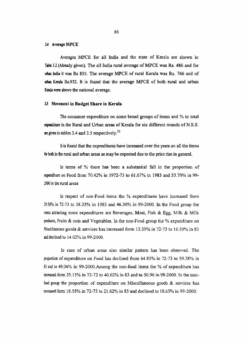
86
14 Average MPCE
Averages MPCE for all India and the state of Kerala are shown in
Table 3.2 (Already given). The all India rural average of MPCE was Rs. 486 and for
urban India it was Rs 855. The average MPCE of rural Kerala was Rs. 766 and of
urban Kerala Rs.932. It is found that the average MPCE of both rural and urban
KeraIa were above the national average.
3.5 Movement in Budget, Share in Kerala
The consumer expenditure on some broad groups of items and % to total
expenditure in the Rural and Urban areas of Kerala for six different rounds ofN.S.S.
are given in tables 3.4 and 3.5 respectively.23
It is found that the expenditures have increased over the years on all the items
fer both in the rural and wban areas as may be expected due to the price rise in general.
In tenns of % there has been a substantial fall in the proportion of
expenditure on Food from 70.42% in 1972-73 to 61.67% in 1983 and 53.70% in 99-
2000 in the rural areas
In respect of non-Food items the % expenditures have increased from
29.58% in 72-73 to 38.33% in 1983 and 46.30% in 99-2000. In the Food group the
items attracting more expenditures are Beverages, Meat, Fish & Egg, Milk & Milk
products, Fruits & nuts and Vegetables. In the non-Food group the % expenditure on
Miscellaneous goods & services has increased form 13.39% in 72-73 to 16.59% in 83
and declined to 14.02% in 99-2000.
In case of urban areas also similar pattern has been observed. The
proportion of expenditure on Food has declined from 64.85% in 72-73 to 59.38% in
83 and to 49.04% in 99-2000.Among the non-food items the % of expenditure has
increased form 35.15% in 72-73 to 40.62% in 83 and to 50.96 in 99-2000. In the non
food group the proportion of expenditure on Miscellaneous goods & services has
increased form 18.55% in 72-73 to 21.62% in 83 and declined to 18.63% in 99-2000.

87
Table 3.4 Per Capita per month (30 days Expenditure (in Rs.O.OO) of broad groups of Food and non-Food items and % to total expenditure in rural areas of Kerala
Year S. Item Oct.72- Jul77- Jan- July 87- Ju1.93- Julygg-No. Sep.73 Jun -78 Dec83 Jun -88 Jun-94 JunOO
1 0IaI Cereals PC 13.49 17.6 34.86 37.83 66.46 110.68
% 31.97 23.71 24.01 17.89 17.53 14.45
2 ~,ram PC 0.04 0.14 0.25 0.46, 1.06 1.87 % 0.09 0.19 0.17 0.22 0.27 0.24
3 ~s Substitute ~E 2.3 2.1 2.34 2.8 4.19 4.78 % 5.45 2.83 1.61 1.32'. 1.07 0.62
4 Pulse & pulse products PC 0.54 1.12 2.34 3.69" 7.2 13.47
% 1.28 1 fi1 1 R1 1.74 1.84 1.76
5 • & Milk products PC 1.52 3.07 5.97 9.76 20.39 37.88
% 3.6 4.14 4.11 4.62 5.22 4.95
6 k:dilIe oil PC 0.82 1.58 3.96 6.76 11.3 20.22 % 1.94 2.13 2.73 3.2 2.89 2.64
7 ~ Eggs, and Fish PCE 1.92 4 8.97 15.59 33.01 61.33 % 4.55 5.39 6.18 7.37 8.46 8.01
8 ~tabIes PC 0.94 1.73 4.13 7.48 16.27 29.53 % 2.23 2.33 2.84 3.54 4.17 3.86
9 ruils & Nuts dry Fruits feE 1.79 3.86 8.12 14.38 23.9 38.51 % 4.24 5.2 5.59 6.8 6.12 5.03
10 Sugar PC 1.51 1.51 2.94 4.58 9,96 12.07
, % 3.58 2.03 2.02 2.17 2.55 1.58 I
111 Salt PC 0.07 0.1 0.16 0.22 0.46 1.02
% 0.17 0.13 0.11 0.1 0,12 0.13 ! PC 1.23 2.52 3.49 6.42 10.22 19.69 112 ~ : % 2.92 3.4 2.4 3.04 2.62 2.57 ! ,- ~verages etc
PC 4 6.09 11.71 16.75 29.62 60.16 ! IJ
% 9.48 8.21 8.06 7.92 7.59 7.86 I
i 14 ood Total IPc 29.71 45.42 89.54 126.76 236.03 411.19
! % 70.42 61.2 61.67 59.94 60.46 53.7
115 Pan, Tobacco & intoxicants IPC 1.58 2.55 4,5 6.79 13.01 19.11
% 3.74 3.44 3.1 3,21 3.33 2,5 I IPCE 2.48 4.4 8.45 13.53 22.41 45,9 . IS uel & light ! % 5.88 5.93 5.82 6.4 5.74' 5.99 i
~101hing PC 1.78 5.38 9.27 10.78 16.8 42,62
i17 I % 4.22 7.25 6.38 5.1 4.3 5.57
! 18 ootwear PC 0.05 0.26 0.95 1.55 3,54 6.06
I % 0.12 0.35 0.65 0.73 0.91 0.79
i 19 ~sc, goods & services !PC 5.65 11.7 24.09 38.78 78.39 107.34
l % 13.39 15.76 16.59 18.34 20.08 14,02
I~ ~on.Food !PC 12.48 28.98 55.66 84.76 154.38 354.51 I % 29.58 39.05 38.33 40.08 39.54 46.3
21 olal Consumer expenditu PC 42.19 74.22 145.2 211.47 390.41 765.71 % 100 100 100 100 100 100
SM:e: NSSO different rounds.

88
Tabla 3.5 Per Capita per month (30 days Expenditure (in Rs.O.OO) of broad groups of Food d F d I d't' U b f K I an non- 00 items and '10 to tota expen I ure In r an areas 0 era a
! Year -
!1No Item Oct.72- Juln- Jan-Dec July 87- Jul.93- July 99-Sep73 Jun -78 83 Jun -88 Jun-94 Jun-OO
1 0taI Cereals PCE 14.16 16.7 35.18 35.82 64.13 105.74 % 24.3 20.19 19.95 13.46 12.99 11..34
2 ~ PCE 0.07 0.22 0.4 0.67 1..55 2.54 % 0.1? 0.27 0.22 0.25 0.31 0.27
3 ~Substitute PC 1.26 1.03 0.78 0.85 1.86 2 .. 22 % 2.16 1.25 0.44 0.32 0.38 0 .. 24
4 Pulse & Pulse Products PC 1.03 1.5 3.02 5.06 8.07 16.98 % 1.n 1.81 1.71 1.9 1.63 1.82
5 ~ & Milk products PC 3.06 4.35 9.02 16.27 27.67 49.27 % 5.25 5.26 5.11 6.11 5.6 5.82
6 ~oil PC 1.25 2.04 5.04 8.53 12.74 23 % 2.15 2.47 2.86 3.2 2.58 2.47
7 ~~ Eggs, and Fish PC 2 .. 96 4.n 11.62 21.24 40.04 70.38 % 5.08 5.n 6.59 7.98 8.11 7.55
I 8 ~tabIes PC 1.28 :1.98 4.99 8.97 16.92 33.22 % 2.2 2.39 2.83 3.37 3.43 3.56
! 9 ~ruits & Nuts Dry Fruits PC 2.46 4.6 9.76 17.54 27.1 42.18 % 4.22 5.56 5.53 6.59 5.49 4.51
i 10 ~ar PC 1.64 1.81 3.39 5.11 10.82 12.48 L % 2.81 2.19 1.92 1.92 2.19 1.34
111 ~t PC 0.06 0.09 0.14 0.24 0.52 1.06 % 0.1 0.11 0.08 0.09 0.11 0.11
I
~ PC 1.34 2.53 3.76 6.49 9.97 20.1
l12 % 2.3 3.06 2.13 2.44 2.02 2.16
! 13 ~verages ete PC 7.22 9.35 18.44 25.19 44.n 78.28 I % 12.39 11..3 10.46 9.46 9.97 8.39
: 14 oodTotal PC 37.79 50.97 104.73 159.2 266.27 457.35 % 64.85 61.61 59.38 59.79 53.92 49.04
I 15 Pan. Tobacco & intoxicants PC 1.92 2.38 4.23 5.48 11.9 18.59 I % 3.3 2.88 2.4 2.06 2.41 1.99
i 16 uel & light PC 3.15 5.2 10.23 16.02 27.38 54.29 % 5.41 6.29 5.8 6.02 5.54 5.82
17 ~Iothing PC 2.83 5.75 14.35 12.86 36.21 53.84 % 4.86 6 .. 95 8.14 4.83 7 .. 33 5.77
; 18 ootwear PCE 0.15 0.4 1.69 2.69 4.81 8 .. 56 % 0.26 0.48 0.96 1.01 0.97 0.92
19 Mise. good & Services PCE 10.81 13.55 38.13 56.87 122.61 173.75 % 18.55 16.38 21.62 21.36 24.83 18.63
20 Non-Food PC 20.48 31.76 71.63 114 .. 3 227.55 475.26 % 35.14 38.38 40.61 42.91 46.07 50.96
I
PC 58.27 82.73 176.36 266.22 493.83 932.62 I 21 olal Consumer Expenditur
% 100 100 100 100 100 100 SMe: NSSO different rounds.
Looking at the latest round data given here for Kerala, a picture of
"average" rural and urban consumption patterns for the state as a whole emerges. The
following are the main features.

89
For rural K.erala per capita 30 'days' consumer expenditure was split up into
53.7% for Food and 46.3% for non-Food. Food included 14.05% for Cereals, and 5% for
Fruits & nuts, 8% for Meat, Fish & Eggs, 7.86% on Beverages and 5% for Milk & Milk
poducts. 3.86% were spent on Vegetables. Non-Food included 6% for Fuel & light and
557'10 for Clothing and only 0.79«'10 on Footwear. Miscellaneous goods & services
constituted 14.02% for rural Kerala. Pan, Tobacco & intoxicants constituted 2.5%.
For the urban sector average MPCE was split up into 49% for Food and
50.96% for non-Food. Of Food expenditure only 11.34% went toward Cereals. While
839% was on Beverages and 7.55% on Meat, Fish & Eggs., 5.82% was spent on
Milk & Milk products, 4.51 % on Fruits & nuts and 3.56% on Vegetables.
5.82% was spent per person on Fuel & light, 5.77% on Clothing and
0.92% on foot wear. Miscellaneous goods & services constituted 18.63%. 1.99% was
spent on Pan, Tobacco & intoxicants. Table 3.6 gives rural urban differences in the %
of per capita consumption of different groups of items in Kerala.
Table 3.6 Rural Urban differences in the value of per capita consumption of different f 't . K I b d 55th d groups 0 I ems In eraa. ase on roun
SI. % expenditure per persons over 30
Difference Items group day period No.
Rural Urban urban-rural %
, Cereals 14.45 11.34 -3.11 2 Pulses 1.76 1.82 0.06 3 Milk 4.95 5.82 0.87
• Edible oil 2.64 2.47 -0.17 5 Meat Eggs and Fish 8.01 7.55 -0.46 6. Vegetables 3.86 3.56 -0.3 7 Fruits & nuts 5.03 4.51 -0.52 8 Sugar 1.58 1.34 -0.24 9 Beverages 7.86 8.39 0.53 10. All Food 53.7 49.04 -4.66
" Pan, Tobacco, intoxicants 2.5 1.99 -0.51
'2. Fuel & light 5.99 5.82 -0.17 13 CIolhing 5.57 5.77 0.2 14. Footwear 0.79 0.92 0.13 19. Mise: goods and service total 14.02 18.63 4.61 21 All non-Food 46.3 50.96 4.66 22. Total consumer expenditure 100 . 100 0
Wai. NSSO different rounds.

90
Rural expenditure % exceeded urban levels among food items for cereal and
tmal substitutes, Edible oil, Meat, fish & egg, Vegetables, Fruits & nuts and Sugar. For
!be itans Pulses, Milk and Beverages urban expenditure % exceeded rural levels.
Non-Food expenditure per person was found higher in the urban sector than in
the rural. Among non-food,hems for items Pan, tobacco & intoxicants, and Fuel &
light % of rural expenditure exceeded that of urban and for all other non-food items
urban expenditure was high~~ .
l' ,., .. ",_ ..... e .. DU'dget share In Indlea •• " •• &v, ....... ""aa .. &.. ... .
The consumer expenditure on some broad groups of items and % to total
expenditure in the Rural and Urban areas of India for six different rounds of N.S.S.
ue given in tables 3.7 and 3.8 respectively.24
It is found that the expenditures have increased over the years on all the
items for both in the rural and urban areas as may be expected due to the price rise in
general. In tenns of % there has been a substantial fall in the proportion of
expenditure on Food from 72.81% in 1972-73 to 65.57% in 1983 and to 59.4% in
1999·2000 in the rural areas
In respect of non-Food items the % expenditure has increased from
27.19% in 1972-73 to 34.42% in 1983 and 40.60% in 1999-2000. In the Food group
the items attracting more expenditure are Milk and Milk products, Vegetables, meat,
Eggs and Fish, Edible oil and Beverages. In the non-Food group, the % expenditure
on Miscellaneous goods & services has increased from 8.89% in 1972-73 to 12.74%
and declined to 11.61 % in 1999-2000.
In case of urban areas also similar pattern has been observed. The
proportion of expenditure on Food has declined from 64.49% in 1972-73 to 59.12%
in 1983 and 48.06% in 1999-2000. In the non-Food group, the proportion of
expenditure on Miscellaneous goods & services has increased form 19.22 % in 1972-
i3 to 24.45% in 1983 and 22.06% in 1999-2000
Looking at the latest round data given here, a picture of "average" rural
and urban consumption patterns for the country as a. whole emerges. The following
are the main features.
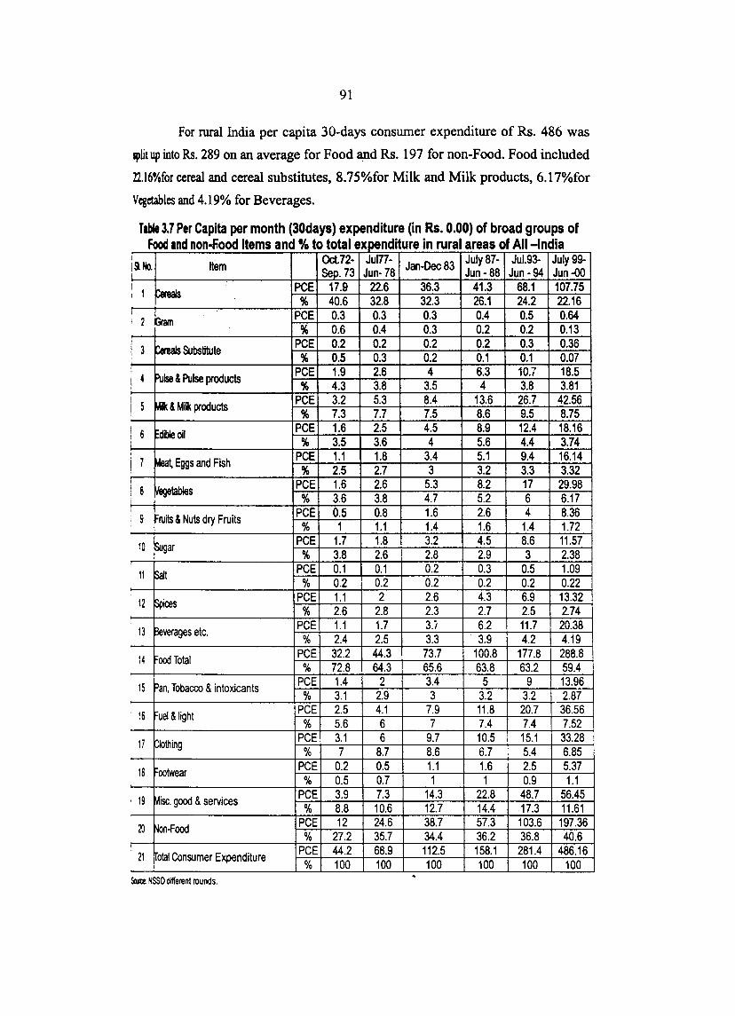
91
For rural India per capita 30-days consumer expenditure of Rs. 486 was
,lit up into Rs. 289 on an average for Food and Rs. 197 for non-Food. Food included
22.l6%for cereal and cereal substitutes, 8.75%for Milk and Milk products, 6.17%for
Vegetables and 4.19% for Beverages.
Table 3,7 Per Capita per month (30days) expenditure (in Rs, 0.00) of broad groups of Food d fi" od i d ~ I d't I I f All I d' an non- 0 tems an o to tota expan lure n rura areas 0 -n la
I
ltern 0cl72- Juln- July 87- Jul.93- July 99-
liNo. Sep.73 Jun-78 Jan-Dec83 Jun - 88 Jun -94 Jun -00
! 1 ~ PCE 17.9 22.6 36.3 41.3 68.1 107.75 % 40.6 32.8 32.3 26.1 24.2 22.16
, Gram PCE 0.3 0.3 0.3 0.4 0.5 0.64
I 2 % 0.6 0.4 0.3 0.2 0.2 0.13
I ~Substitute PCE 0.2 0.2 0.2 0.2 0.3 0.36 l 3 % 0.5 0.3 0.2 0.1 0.1 0.07
I 4 Pulse & Pulse products PCE 1.9 2.6 4 6.3 10.7 18.5 % 4.3 3.8 3.5 4 3.8 3.81
I 5 la & Milk products PCE 3.2 5.3 8.4 13.6 26.7 42.56 % 7.3 7.7 7.5 8.6 9.5 8.75
I 6 ~ibIe oil PCE 1.6 2.5 4.5 8.9 12.4 18.16 i % 3.5 3.6 4 5.6 4.4 3.74 , PCE 1.1 1.8 3.4 5.1 9.4 16.14 i 7 ~ Eggs and Fish
% 2.5 2.7 3 3.2 3.3 3.32 , 8 ~1abIes PCE 1.6 2.6 5.3 8.2 17 29.98
! % 3.6 3.8 4.7 5.2 6 6.17 I
9 Fruits & Nuts dry Fruits PCE 0.5 0.8 1.6 2.6 4 8.36 I
% 1 1.1 1.4 1.6 1.4 1.72
10 ~gar PCE 1.7 1.8 3.2 4.5 8.6 11.57 , % 3.8 2.6 2.8 2.9 3 2.38
11 ~II PCE 0.1 0.1 0.2 0.3 0.5 1.09 I % 0.2 0.2 0.2 0.2 0.2 0.22
12 ~s PCE 1.1 2 2.6 4.3 6.9 13.32 % 2.6 2.8 2.3 2.7 2.5 2.74
13 ~verages elc. PCE 1.1 1.7 3.; 6.2 11.7 20.38 % 2.4 2.5 3.3 . 3.9 4.2 4.19
14 ood Total PCE 32.2 44.3 73.7 100.8 177.8 288.8 % 72.8 64.3 65.6 63.8 63.2 59.4
; 15 Pan, Tobacco & intoxicants PCE 1.4 2 3.4 5 9 13.96 % 3.1 2.9 3 3.2 3.2 2.87
, 16 uel & light PCE 2.5 4.1 7.9 11.8 20.7 36.56 % 5.6 6 7 7.4 7.4 7.52
17 Pothing PCE 3.1 6 9.7 10.5 15.1 33.28 % 7 8.7 8.6 6.7 5.4 6.85
18 oolwear PCE 0.2 0.5 1.1 1.6 2.5 5.37 % 0.5 0.7 1 1 0.9 1.1
, 19 ~isc. good & services PCE 3.9 7.3 14.3 22.8 48.7 56.45 % 8.8 10.6 12.7 14.4 17.3 11.61
20 Non-Food PCE 12 24.6 38.7 57.3 103.6 197.36 % 27.2 35.7 34.4 36.2 36.8 40.6
21 ~otal Consumer Expenditure PCE 44.2 68.9 112.5 158.1 281.4 486.16 % 100 100 100 100 100 100
Some: NSSO different rounds.

92
TiIiI 3.8: Per Capita per month (30 days Expenditure (in Rs.O.OO) of broad groups of F d F d' d % I d't' U ba f All I d' ood an non· 00 items an to tota expan I ure In r n areas 0 • n la
Oct.72- Juln-.
July 87- Ju1.93- July 99-iNa. Item ~an-Dec83 Sep.73 Jun-78 Jun-88 Jun-94 Jun-OO
, Iroli Cereals PCE 14.8 19.7 32 37 64.3 105.57 % 23.3 20.4 19.5 14.8 14 12.35
2 Gm PCE 0.2 0.2 0.3 0.4 0.8 0.95 % 0.3 0.2 0.2 0.2 0.2 0.11
J Cereas Substitute PCE 0.1 0.1 0.1 0.2 0.3 0.35 % 0.1 0.1 0.1 0.1 0.1 0.04
• Nse & Pulse Products PCE 2.2 3.4 5.3 8.4 13.9 24.25 % 3.4 3.6 3.2 3.4 3 2.84
5 ~ & MUk products PCE 5.9 9.2 15.2 23.8 44.9 74.17 . _ .. % 9.3 9.5 9.2 9.5 9.8 8.68
6 Edible oil PCE 3.1 4.5 7.9 13.2 20.1 26.81 % 4.8 4.6 4.8 5.3 4.4 3.14
7 Meal Eggs, and Fish PCE 2.1 3.3 5.9 8.9 15.5 26.78 % 3.3 3.5 3.6 3.5 3.4 3.13
8 \legetables PCE 2.8 4.2 8.2 13.1 25 43.9 % 4.4 4.4 5 5.2 5.5 5.13
9 ruits & Nuts dry Fruits PCE 1.3 1.9 3.5 6.3 10.2 20.68 % 2 2 2.1 2.5 2.2 2.42
10 Sugar PCE 2.3 2.5 4 5.9 11 14 % 3.6 2.6 2.5 2.3 2.4 1.64
" Salt
PCE 0.1 0.1 0.2 0.3 0.6 1.38 % 0.1 0.1 0.1 0.1 0.1 0.16
'2 ~ PCE 1.4 2.4 3.3 5.5 8.8 17.73 % 2.2 2.5 2 2.2 1.9 2.07
13 ~verages ete PCE 4.8 6.1 11.2 16.8 33 54.28 % 7.6 6.3 6.8 6.7 7.2 6.35
~~ cod Total PCE 40.8 57.7 97 139.8 250.3 410.84 % 64.5 60 59.1 55.9 54.7 48.06
15 Pan. Tobacco & intoxicants PCE 1.8 2.3 4 6.5 10.7 16.22 % 2.8 2.4 2.4 2.6 2.3 1.9
16 uel & light PCE 3.6 6.2 11.4 16.7 30.2 66.26 % 5.6 6.4 6.9 6.7 6.6 7.75
17 ~Iothing PCE 3.3 6.8 12.5 15 21.4 51.76 % 5.3 7.1 7.6 6 4.7 6.05
18 ootwear PCE 0.3 0.6 1.8 2.7 4.2 10.05 % 0.4 0.6 1.1 1.1 0.9 1.18
19 Mise. good & Services PCE 12.17 17.9 40.11 58.64 126.03 188.6 % 19.22 18.62 24.45 23.46 27.52 22.06
~ Non·Food PCE 22.5 38.5 67.1 110.2 207.7 444.08 % 35.5 40 40.9 44.1 45.3 51.94
21 otal Cons. Expenditure PCE 63.3 96.2 164 249.9 458 854.92 % 100 100 100 100 100 100
)w: NSSO Different Rounds
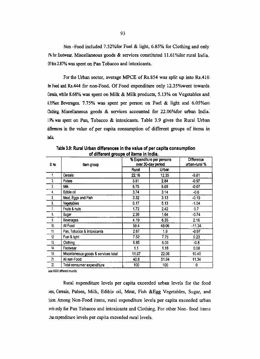
93
Non -Food included 7.52%for Fuel & light, 6.85% for Clothing and only
1% for footwear. Miscellaneous goods &. services constituted 11.61 %for rural India.
Of this 2.87% was spent on Pan Tobacco and intoxicants.
For the Urban sector, average MPCE of Rs.854 was split up into Rs.410·
for Food and Rs.444 for non-Food. Of Food expenditure only 12.35%went towards.
Cereals, while 8.68% was spent on Milk & Milk products, 5.13% on Vegetables and
6.3So/00n Beverages. 7.75% was spent per person on Fuel & light and 6.05%011
Clothing. Miscellaneous goods & services accounted for 22.06%for urban India~
1.9'1. was spent on Pan, Tobacco & intoxicants. Table 3.9 gives the Rural Urban
differences in the value of per capita consumption of different groups of items in
India.
Table 3.9: Rural Urban differences In the value of per capita consumption f d·ff t f It i I d' 0 I eren: groul )50 ems n n la.
% Expenditure per persons Difference SI. No Item group over 3O-day period. urban-rural %
Rural Urban 1. Cereals 22.16 12.35 -9.81 2. Pulses 3.81 2.84 -0.97 3. Milk 8.75 8.68 -0.07 4. Edible oil 3.74 3.14 -0.6 5. Meat, Eggs and Fish 3.32 3.13 -0.19 6. Vegetables 6.17 5.13 -1.04 7. Fruits & nuts 1.72 2.42 0.7 8. Sugar 2.38 1.64 -0.74 9. Beverages 4.19 6.35 2.16 10. All Food 59.4 48.06 -11.34 11. Pan, Tobacco & Intoxicants 2.87 1.9 -0.97 12. Fuel & light 7.52 7.75 0.23 13. Clothing 6.85 6.05 -0.8 14. Footwear 1.1 1.18 0.08 19. Miscellaneous gOOdS & services total 11.67 22.06 10.45 21. All non-Food 40.6 51.94 11.34 22. Total consumer expenditure 100 100 0
)w: NSSO different rounds
Rural expenditure levels per capita exceeded urban levels . for the food
,lCIIlS, Cereals, Pulses, Milk, Edible oil, Meat, Fish &Egg Vegetables, Sugar, and
Spices. Among Non-Food items, rural expenditure levels per capita exceeded urban
tI'CIs only for Pan Tobacco and intoxicants and Clothing. For other Non- food items
~rban expenditure levels per capita exceeded rural levels.

94
17 Food Expenditure Pattern in Kerala
Analysis of the per capita expenditure on individual items of Food in
rdaIion to total Food expenditure will show clearly how total Food expenditure is
IIIocated and the changes in consumption pattern. The following two tables 3.10 and
Table 3.11,. Present per capita per month expenditure on broad groups of Food items
and % to total Food expenditure in rural and urban areas ofKerala.
The table 3.10 reveals that in the rural sector the % of expenditure on
C:reals has declined form 45.41 % in 1972-73 to 38.93% in 1983 and 26.92% in 99-
2000. The increase in % expenditure has been observed in respect of Milk & Milk
IIOCfucts, Pulses, meat Eggs & Fish and Vegetables. The % of expenditure on Fruits
1 nuts has increased from 6.02% in 72-73 to 9.37% in 99-2000. The % expenditure
011 Edible oil has increased fonn 2.76% in 72-73 to 4.92% in 99-2000. The % of
expenditure on Sugar has declined from 5.08% in 72-73 t02.94 in 99-2000. The % of
apmditure on Salt has declined form 0.24% in 72-73 to 0.29% in 99-2000.
The % of expenditure on Spices has increased from 4.14 % in 72-73 to
4.79% in 99-2000. As different from all - India pattern, the % of expenditure on
Beverages has declined form 13.46% in 1972-73 to 13.08% in 1983, and then
llICreased to 14.63% in 99-2000.
Table 3.10: Percentage expenditure on different items of Food to total F d d't K I R I 00 ex pen lure era.3- ura.
s. No. Item Qct 72· Jul77· Jan· Jul87 - Ju193· June June99· Sep73 June 78 Dec83 June 88 94 July 2000 , alal Cereals % 45.41 38.75 38.93 29.84 29.00 26.92
2 Gram % 0.13 0.31 0.28 0.36 0.45 0.24 3 Cereals Substitutes % 7.74 4.62 2.61 2.21 1.78 1.16 , Pulses & Pulse Products % 1.82 2.47 2.61 2.91 3.05 3.28 5 Milk & Milk products % 5.12 6.76 6.67 7.70 8.64 9.21 0 dibleoil % 2.76 3.48 4.42 5.33 4.79 4.92 7 Meal Eggs and Fish % 6.46 8.81 10.02 12.30 13.99 14.96 8 Vegetables % 3.16 3.81 4.61 5.90 6.89 7.18 9 ruits & nuts, dry Fruits % 6.02 8.50 9.07 11.34 10.13 9.37 10 Sugar % 5.08 3.32 3.28 3.61 4.22 2.94
l' Salt % 0.24 0.22 3.50 0.17 0.19 0.29 12 Spices % 4.14 5.55 3.90 5.06 4.33 4.79 13 ~verages etc % 13.46 13.41 12.08 13.21 12.55 14.63 14 ood Total % 100.00 100.00 100.00 100.00 100.00 100.00
).w: NSSO different rounds

95
The table 3.11 reveals that in the urban sector, the % expenditure 'on
CaeaJsbasdeclined fonn 37.47% in 1972-73 to 23.12% in 99-2000. The increase in
"expenditure has been observed in respect of Milk & Milk products, Pulses, Meat,
F1h & Eggs, and Spices. The % of expenditure on Edible oil has increased from
331% in 72-73 to 5.03% in 93-94.
Table 3,11: Percentage expenditure on different items of Food to total F od d't K I rba 0 expen lure era a-u n
Round (Year)
SI«! Item Oct72- Juln- Jan- Jul87 - Ju193- June99-Sep73 June 78 Dec83 June 88 June 94 July 2000
1 0taI Cereals % 37.47 32.76 33.59 22.50 24.08 23.12 2 Gnrn % 0.19 0.43 3.22 0.42 0.58 0.56 3 peraas Subs~tutes % 3.33 2.02 0.74 0.53 0.70 0.49 4 pwses & Pulse Products % 2.73 2.94 2.88 3.18 3.03 3.71 5 ta & Milk products % 8.00 8.53 8.61 10.22 10.39 10.78 6 ElIlIeoil % 3.31 4.00 4.81 5.36 4.78 5.03 7 ~ Eggs and Fish % 7.83 9.36 11.18 13.34 15.04 ' 15.38 8 % 3.39 3.88 4.76 5.64 6.35 7.26 9 ruiIs & nuts, dry Fruits % 6.51 9.02 9.32 11.02 10.18 9.20 10 • % 4.34 3.55 3.24 3.21 4.06 2.79 11 SIt % 0.16 0.18 0.13 0.15 0.20 0.23 ~2 ~ % 3.55 4.96 3.59 4.08 3.70 4.39 13 ~etc % 19.12 18.34 17.61 15.83 16.81 17.16 :4 ood Total % 100.00 100.00 100.00 100.00 100.00 100.00
_ NSSO dIIerent rounds.
The % of expenditure on Sugar has declined from 4.34%in 72-73 to
: ~9% in 99-2000. The % of expenditure on Salt has increased from 0.16% in 72-73
:.v 0.23% in 99-2000. The % of expenditure on Beverages in urban Kerala declined
::om 19.11 % in 72-73 to 17.16 % in 99-2000. Among Condiments & Spices,
~::rmeric, Black pepper, Tamarind and Ginger are the few items having Homegrown
hock consumption in urban areas of Kerala, which constitutes 2% of the total per
:Jflta consumption of Condiments and Spices in urban Kerala.
jJ Food Expenditure Pattern in India
Analysis of the per capita expenditure on individual items of Food in
~;ation to total Food expenditure will show clearly how total Food expenditure is
l.:ocated and also the changes in consumption pattern. the following tables 3.12 and

96
3.13 present % expenditure on items of Food to total Food expenditure in the rural
lid urban areas of India.
liNo. I
I 1 I
I 2 ; 3 i 4 . i ~
l 6 I 7 I 8
I 9 i 10
~ 11
: 12 , 13
. 14
Table 3.12: Percentage expenditure on different items of Food to total Food expenditure India - Rural.
Item Oct.72-Sep.73 . Ju177- Jan-Dec83 July 87- Ju1.93-Jun-78 Jun-88 Jun-94
lrotalCerUs 55.7 I.
51 49.2 41 38.3
~ 0.8 . 0.7 0.4 0.4 0.3
~ Substitutes 0.7 . 0.5 0.3 0;2 0.2
Pulses & Pulse Products 5.9 .' 5.9 5.4 6.2 6
~ ci :vuiA .,.uJu~l=t iO 11.9 11.5 13.5 15
~oiI 4.8 5.5 6.1 8.8 7
• Eggs and Fish 3.4 4.2 4.6 5.1 5.3
-11' 4.9 5.9 7.2 8.2 9.6
ruits & nuts. dry Fruits 1.4 1.7 2.1 2.5 2.3
Sugar 5.2 4.1 4.3 4.5 4.8
Salt 0.3 0.3 0.3 0.3 0.3
Spices 3.5 4.4 3.6 4.2 3.9
Beveragesetc 3.3 3.9 5 6.1 6.6 I:ood Total 100 100 100 100 100
_ NSSO dillerent rounds
June 99-Jul-OO 37.3
0.22
0.12
6.4
14.7
6.28
5.58
10.3
2.89
4.01
0.37
4.61
7.05
100
It is found that in the rural sector the % expenditure on Cereals has
declined from 55.72% in 1972-73 to 37.3% in 99-2000.
The % of expenditure on Milk & Milk products has declined from 10% in
1972-73 to 4.7% in 99-2000. The % of expenditure on Edible oil has increased from
4.8% in 72-73 to 6.28% in 1999-2000. Increase in % expenditure has been observed
in respect of Meat, Fish & Eggs, 3.39% in 1972-73 to 5.58% in 99-2000. Increase in
'4 expenditure has been observed in case of Vegetables also 4.94% in 72-73 to 10.3%
in 99-2000. For Fruits & nuts also increase in % expenditure has been observed, 1.4%
in 72-73 to 2.89% inI999-2000. Increase in % expenditure on Beverages has been
observed, 3.33% in 72-73 to 7.05% in 99-2000.
In the urban sector increase in % expenditure has been observed for Milk
& Milk products 14.47% in 72-73to 18.05% in 99-2000, Vegetables 6.78% in 72-73
to 10.68% in 99-2000,Fruits & nuts 3.11 % in 72-73 to 5.03% in 99-2000. % of
expenditure on Beverages has increased from 11.80% in 72-73 to 13.21 % in 99-2000.

IS-No.
I 1 l 2
3 4 5 6 7 8 9
I 10 I 11 I 12
13 14
97
Table 3.13: Percentage expenditure on different items of Food to total Food expenditure. India - Urban.
Item 0cl72- Jul77- Jan-Dec83 July 87- Ju1.93-Sep73 June 78 June- 88 Jun94
0taI Cereals 36.17 34.09 32.96 26.45 25.68 Grmn 0.49 0.42 0.33 0.29 0.34 ~ Substitutes 0.2 0.17 0.13 0.12 0.12 Pulses & Pulse Products 5.29 5.95 5.46 6.04 5.56 • & Milk products 14.47 15.88 15.62 17.05 17.93 ~oiI 7.52 7.73 8.19 9.47 8.03 ~ Eggs and Fish 5.07 5.77 6.1 6.33 6.2 ~tabIes 6.78 7.33 8.43 9.39 9.99 Nits & nuts, dry Fruits 3.11 3.26 3.57 4.49 4.07
~ 5.58 4.4 4.16 4.19 4.39 ~ 0.17 0.23 0.19 0.21 0.25 ~ 3.35 4.2 3.43 3.22 3.51
ete 11.8 10.56 11.56 12.04 13.19 ood Total 100 100 100 100 100
s.a: NSSO diIIeIant rounds
3.9 Per capita consumption of individual items in India: Food items.
June 99-Juloo 25.69 0.23 0.09 5.9
18.05 6.52 6.57 10.68 5.03 3.4 0.36 4.32 13.21 100
Per capita expenditure estimates for different items of consumption
including Food, Pan, Tobacco & intoxicants and Fuel, Clothing & Footwear
Education and Medical expenses and other Miscellaneous items are presented based
on different rounds ofNSS data.
Table 3. 14 and 3.15 shows the quantity and value of total consumption of
different items of Food, Pan, Tobacco & intoxicants and Fuel & light per person for a
period 000 days during 1987-88. 1993-94 and 1999-2000 for All India, for the rural
and urban sectors. These tables are presented Appendix
3.9.1 Cereals and Pulses
All India consumption of Atta has declined from 4.48kg in 87-88 per
person for 30 days to 4.32 kg in 93-94 and increased to 4.45 kg in 1999-2000 in rural
areas. While for the urban sector rise was observed, from 4.37 kg in 87-88 to 4.44 kg
in \993-94 and to 4.45 kg in 99-2000. In the rural sector per capita consumption of
Rice has declined from 6.81 kg in 87-88 to 6.79 kg in 93-94 and to 6.59 kg per person
for a period of 30 days in 99-2000.

98
In the urban sector Rice consumption per person showed a decline from
S16kg in 87-88 to 5.13kg in 93-94 and to 5.10 kg in 99-2000. The decline in Rice
coosumption was more pronounced in rural sector (0.20 kg) than urban (0.03 kg)
bdween 93-94 and 99-2000. Similarly the rise observed in the consumption of Atta
was higher in rural sector (0.32kg) between 93-94 and 99-2000 while the rise
observed irithe urban sector was (0.15kg) lower than that. The per capita
COIISUIDption of Pulses remained stable in rural areas, a marginal rise in consumption
of most of the varieties appears to be indicated in the urban sector.
3.9.2 Milk & MOk products.
The per capita consumption per month has increased by about 600-700 ml
in both sectors during 87-88 to 93-94 but it was under 4 liters (about 130ml per day)
in rural areas and under 5 liters (about 165 ml per day) in Urban areas. One third of
rura1 households and one fifth of all urban households reported no consumption of
Milk during the last 30 days.
These proportions have not changed greatly since the 87-88. In the rural
sector per capita consumption of Milk per month increased since 93-94 by about
ISOmI. It still continues to be less than 4 liters in rural areas and just above 5 liters in
urban areas. In the urban sector per capita consumption per month increased since 93-
94 by about 21 Oml, that is between 93-94 and 99-2000.
3.9.3 Edible oil
It is found that per capita consumption of the item in the urban sector is much
higher than the same in rural sector. All India estimates of per capita consumption of
Edible oil are higher in 99-2000 than in 1993-94. In the urban sector the difference is
much pronounced. Table 3.16 gives Edible oil (gm) consumed per person in 30 days
for India.
Table 3.16. Edible oil (gm) consumed per person in 30 days.
Year Rural Urban
1993-94 340 460
99-2000 410 . 560
SMe: NSSO Different Rounds.

items. At the all-India level, Consumption of meat includes mainly three categories:
pi meat, mutton and Chicken. All India estimates of per capita consumption of
meat are higher in1999-2000 than in 93-94. While in the rural sector per capita
CODSIID1ption of meat has increased from 120 gm per head per month in 1993-94 to
lSOgm in 99-2000, in the urban sector the per capita consumption has increased from
200 gIllS in 1993-94 to 240 gms in 99-2000.
All India estimates of per capita consumption of Eggs shows that, per
capita consumption of Eggs has increased from 0.64 Eggs per person in the rural
s«tor in 93-94 to 1.09 Eggs in 99-2000. In the urban sector the increase was more
pronounced that is from 1.48 Eggs in 93-94 to 2.06 Eggs in 99-2000. Both rural and
urban areas show some increase in per capita consumption of Fish.
3.9.5 Vegetables
Per capita consumption of potato's, onion, cauliflower, cabbage, ladies
finger, tomato, chilly & lemon were higher during 1999-2000 in both rural and urban
areas than during 1993-94. On the whole per capita consumption levels of Vegetables
appear to have risen slightly
3.9.6 Fruits & Duts
The Food group Fruits & nuts showed a marked rural-urban differential as
measured by the % of households reporting consumption last month. Among
Individual items the rural-urban differential in this % is now seen to be as high as
25% points for bananas, 17 for apples and 4-6 points for groundnuts, mangos and
Coconuts. % of households reporting consumption have increased for bananas and
apples and remained stable or fallen slightly for Coconuts and-mangoes.
It may be noted that bananas and Coconuts accounted for 75% of the
\'alue of consumption of fresh Fruits & nuts by rural households in 93-94 and the
corresponding figure was 68% in 99-2000. In the urban sector bananas and Coconuts
accounted for 62% of the value of consumption of fresh Fruits & nuts by urban
households in 93-94, and the corresponding figure was 60% in 99-2000. Table3.17
~ves Consumption of important Fruits & nuts in India.

100
Table 3.17: Consumption of important Fruits & nuts. Rural Urban
% Of households Value of per capita % Of households Value of per capita FftIII&1KIIs reporting consumption consumption Rs in 30 reporting consumption consumption (Rs.) in
,
lastmontah days last month 30 days 87.a8 93-94 93-94 99-2000 87-88 93-94 93-94 99-2000 ... 32 43 1.15 1.90 60 68 2.80 4.40
eau 25, 24 1.23 1.92 31 30 1.89 2.96 .... 9 8 0.40 1.04 14 13 1.30 2.48 ,. 6 9 . . 19 26 2.35 1.62 ,rUtilFnits 56 " 64 4.90 6.89 78 84 12.20 16.67 QQIIdool 10 ' 14 0.48 0.83 18 22 . . _NSSO~rounds. .
3.9.7 Other Food: Sugar
While all India consumption of crystalline Sugar shows an increase of
aly 320gm per month in the rural sector, it is offset by an even sharper fall in per
capita ruraI consumption of Gur, so that the Sugar group as a whole registers little
cbange. Since 1993·94 some substitution of Sugar for Gur appears to have taken
place in the urban sector as well.
1.9.8 Beverages: tea:
While the % of households reporting consumption of purchased tea ("tea:
00. Of cups") has remained stable since 1987-88; the % reporting consumption of tea
tmved at home has gone up by about 6·7 % points. Only about 7 % of the rural
OOIiseholds and 13 % of urban households reported consumption of Coffee powder.
3.10 Per capita consumption of individual items K~rala
3.10.1 Food items
Per capita expenditure estimates for different items of consumption
IOCluding Food, Tobacco, Fuel, Clothing and Footwear, Educational, Medical
expenses and other Miscellaneous items for Kerala are presented for individual item
based on state wise data. Since data on per capita expenditure of individual items
were available only for the latest round of NSS [1999-2000] comparison with earlier
round data cannot be presented for the state. Table 3.18,3.19 gives quantity and value
of per capita purchase and consumption over a 30-day period for important items of
Food for rural and urban Kerala.

I
I
I
i :
I
! !
101
The per capita consumption of Rice in the rural areas of Kerala was
bigher than. the same in the urban areas. Among individual items other items
IIIJ'ICting more per capita consumption in rural Kera1a than urban are consumption of
Vegetables items like Coconut, Salt, Dry chilies, Other Spices, Coffee powder, Salted
Retteshments, Prepared sweets, Cooked meals.
Tlblt118 Monthly per capita quantity and value of consumption. for Food items for Rural Kerala
SI. No Item, 1999 0 2000
Quantity (kg~) . Value (Rs) 1 ~ 9.16 99.47 2 A.tt:! 0;7 6.89
3 ~aI:s.l 9.89 110.68
4 ~aI Substitutes 0.96 4.78
5 Pulse& Pulse Products: S.t 0.55 15.33
6 ~ilk: liquid (Iiter) 2.97 35.91 7 Milk & Milk products: s.l 0 37.88
8 Coconut oil 0.31 1.6.61 9 ~dible oil: S.t 0.42 20.22 10 ~ggs, Fish Meat s.t. 0 61.33 11 ~egetables: s.t 0 29.53 12 ~ana(no) 4.49 5.63
13 ~ut(no) 4.89 27.05 14 I::ruits:(fresh): s.t. 0 37.54 15 I-ruits:(dry): s.t. 0.02 0.97 16 ~gar 0.81 11.55 17 Gur 0.03 0.49 18 Sugar: S.t 0.85 12.07 19 Salt 0.27 1.02 20 urmeric(gm) 24.26 1.23 21 Black pepper (gm) 6.07 1.18 22 Dry chilies (gm) 11.51 5.82 23 Garlic (gm) 25.87 1.01 24 amarind (gm) 72.82 3.35 25 Ginger (gm) 20.94 ·0.79 26 Spices: s.t. 0 19.69 27 ea: Leaf gm) 95.9 23.85 28 Biscuits 0.61 3.03 29 Salted Refreshments 1.52 4.48 30 Prepared sweets 0.09 0.91 31 Cooked meals (no) 1.36 18.36 32 Beverages ete: s.t: 0 60.16 33 Total Food 0 411
SaIa!: NSSO (1999·2000). 'Consumption of some important commodities in India. based on NSS 55111 round. (July 1999· Jun 2000) data •
• No. 461. s.t shows sub total
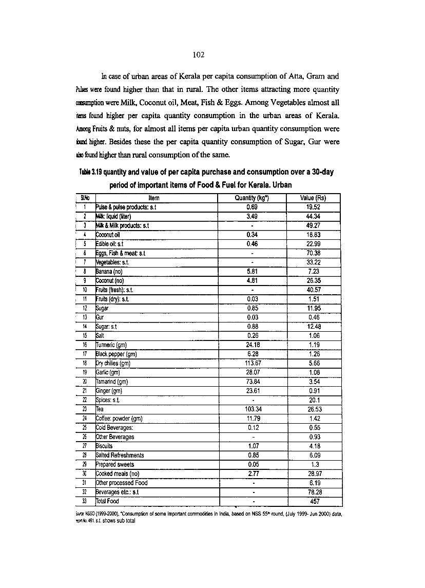
102
In case of urban areas of Kerala per capita consumption of Atta, Gram and
Pulses were found higher than that in rural. The other items attracting more quantity
aaumption were Milk, Coconut oil, Meat, Fish & Eggs. Among Vegetables almost all
itans found higher per capita quantity consumption in the urban areas of Kerala.
Among Fruits & nuts, for almost all items per capita urban quantity consumption were
baMl higher. Besides these the per capita quantity consumption of Sugar, Gur were
IIIl found higher than rural consumption of the same.
I
I
I
I
I
Table 3.19 quantity and value of per capita purchase and consumption over a 30-day
period of important items of Food & Fuel for Kerala. Urban $.No Item Quantity (kg*) Value (Rs) 1 PUlse & pulse products: S.t 0.69 19.52 2 ~Ik: flQuid (Iiter) 3.49 44.34 3 ~ & Milk products: S.t - 49.27 4 ~utoil 0.34 18.83 5 Fdible oil: S.t 0.46 22.99 6 Fggs, Fish & meat: s.t - 70.38 7 ~tables: s.t. - 33.22 8 ~ana(no) 5.81 7.23 9 poconut (no) 4.81 26.35 10 ruits (fresh): S.t. - 40.57 11 ruits (dry): S.t. 0.03 1.51 12 ~gar 0.85 11.95 13 pur 0.03 0.46 14 ~gar: S.t 0.88 12.48 15 ~It 0.26 1.06 16 urmeric (gm) 24.18 1.19 17 Slack pepper (gm) 6.28 1.26 18 Dry chilies (gm) 113.67 5.66 19 Garlic (gm) 28.07 1.08 20 amarind (gm) 73.84 3.54 21 Ginger (gm) 23.61 0.91 22 Spices: s.t. - 20.1 23 ea 103.34 26.53 24 Coffee: powder (gm) 11.79 1.42 25 Cold Beverages: 0.12 0.55 26 Other Beverages - 0.93 27 Biscuits 1.07 4.18 28 Salted Refreshments 0.85 6.09 29 Prepared sweets 0.05 1.3 30 Cooked meals (no) 2.77 28.97 31 Other processed Food - 6.19 32 Beverages etc.: s.t - 78.28 33 otal Food - 457
Sow: NSSO (1999-2000), 'Consumption of some important commodities in India, based on NSS 55" round, (July 1999- Jun 2000) data, ~No 461.5.1. shows sub total

103
111 Per capita consumption of individual items in India
111.1 NOD -Food items.
Tables 3.20,3.21 give per capita expenditure on individual items of Non -
Food for All India These are given in Appendix
1l1.1.1 Pan, Bidis and Cigarettes:
Consumption of Finished pan has shown an increase between 1993-94
Dll999·2000 in rural areas. In case of urban sector consumption of finished pan
I1ItIined between 1993-94 and 1999-2000. In both sectors smoking of Bidis has gone
~n judging by per capita consumption levels between 1993-94 and 1999-2000. It is
Diced that the smoking of Cigarettes in the rural sector has increased during the
IiIIIIe period while for the urban sector the same has shown a decline. Table 3.22
Dlws Consumption of Pan, Bidis and Cigarettes. A11- India
Table 3.22: Consumption of Pan, Bidis and Cigarettes. All-India
Year
1987-88 1993·94 99-2000 IBnS
Per capita % Ofhhs Per capita % Ofhhs Per capita % Ofhhs Consumption reporting Consumption reporting Consumption reporting
(no.) consumption (noj consumption (no,) consumption =r. Fflished) 0.65 10 0.64 10 0.83 27 R
U 1.70 15 1.39 12 1.20 21 Bidis 49.5 47 45.7 45 38.18 62 R
U 38.7 31 32.4 27 22.13 39
~1Ies 1.0 4 0.8 4 0.96 ®
R -U 4.9 13 3.7 11 3.24 .
iw. NSSO (1999-2000). 'Consumption of some important commodities in India. based on NSS 55" round. (July 1999- Jun 2000) dam.
_t«l.~1.
1II.1.2 Fuel & light
Fire wood consumption per month has fallen in urban areas by more than
: Kg per capita. The % of Firewood consuming households has fallen from 45% to
:"%. Electricity consumption per person has risen frpm 2.3 standard units (Kwh) to
~.6 units per month in rural areas and from 9.7 units to 20.9 units in urban areas

104
between 93-94 and 99-2000. Finally the per capita consumption of LPG by Urban
households has risen from· 0.88 to 1.31 between 93-94 and 99-2000. The per capita
consumption ofLPG in rural sector remains to be very little.
3.11.1J Medical, Educational, Rent, Conveyance and other Miscellaneous
Elrenditure , .
Non-Food consumer expenditure is usually divided into" si~ to eight
different heads for the purpose of presentations of NSS estimates,. s~ch' as Clothing,
Fuel & light and Durable goods. Of these the category "Miscellaneous goods &
services" commands the largest share of expenditure in both rural and urban areas in
India. MPCE on this group of item as per NSSO 1999-2000 data was, 28.42% in total
non-Food expenditure in rural areas, and 42.57% in urban areas.
Further, the share of this group has been increasing over time in rural
areas. It has doubled over the period 1972-73 to 1999-2000. Unfortunately, most
items of the Miscellaneous "category, in particular the Consumer services, are not
~enable to measurement of quantities consumed. This make it extremely difficult to
separate out change in level of physical consumption from changes in prices as can be
done a reasonable extent for Food and Clothing and make meaningful comparisons
overtime for such data.
Table 3.23 & 3.24 gives the breakup of monthly per capita expenditure on
Miscellaneous goods & services by a number of sub groups: Amusement, Goods for
personal care & effect, Toilet articles, Sundry articles, Conveyance, Rent, Consumer
taxes and cesses, Educational expenses, Medical expenses and (other) Consumer
services. This break-up is given for each of 12 MPCE classes of population in rural and
urban areas for India.
It is seen that urban households spent nearly four times as much per
person on Educational and three times as much per person on Conveyance as rural
households. Per capita expenditure on Rent was about 5% of total MPCE in urban
areas and only 0.41 % of total expenditure in rural areas. The proportion of MPCE . accounted by Medical expenses appears to be (6% in rural) a little higher in the rural

105
scclor than in the urban, 5%. Also, the importance of Medical expenditure relative to
the other Miscellaneous heads (Education, Conveyance, other consumer services etc)
is seen to be appreciably greater in rural areas compared to urban areas.
Table 3.23 Value (Rs.) of consumption of broad groups of non-Food items per person for a period of 30 days for each MPCE class for Alllndia.Rural
Item ()()(). 225- 255- 300- 340- 380- 420- 470- 525- 615- 775- 950-
I 225 255 300 340 380 420 470 525 615 775 950 more PI! 0.66 1.02 1.17 1.57 2.01 2.40 2.71 3.17 3.47 3.71 4.25 4.15
~ 3.16 4.13 4.74 5.59 6.24 6.82 7.66 8.09 9.02 10.03 11.00 16.95
~Is 1.67 1.73 2.09 2.65 2.54 ... 'u " "" " ~ .. . "" .... n " .. .'" "n .J.U't '.:1, .J.OJI 't.'" ......... u ....... • ".uu
PI!. Tobacro 5.49 6.88 8.01 9.81 10.79 12.25 13.29 14.82 16.72 19.18 23.60 34.09 liaX:crlls
~Ughl 17.45 20.84 23.76 26.25 28.96 31.77 35.39 38.74 43.64 50.85 60.20 75.21
btq 13.92 17.96 20.51 23.ge 25.85 28.71 31.64 34.74 39.22 46.07 54.79 78.70
Fo:tttar 1.39 1.93 2.34 2.96 3.43 3.92 4.69 5.39 6.30 8.00 10.21 20.10
E1taIioo 1.36 2.09 2.98 3.69 4.63 5.42 6.92 8.25 10.75 15.55 23.35 44.61
t.iD:aI-Instituliona 0.55 1.05 1.22 1.66 1.96 2.71 3.56 4.93 7.35 11.17 16.89 45.78
~.jnsl 4.29 6.24 8.21 11.09 12.86 15.34 17.53 21.58 25.76 37.46 49.07 100.45
Erirtinmenl 0.30 0.38 0.60 0.71 1.15 1.43 1.46 1.68 2.20 3.40 4.75 9.78 G.xx!s prs. Care 0.22 0.29 0.47 0.61 0.75 0.71 0.99 1.32 1.64 2.14 3.24 5.74 &eIIeds ~*t articles 4.60 5.74 6.60 7.80 8.86 9.94 10.96 12.31 14.20 16.53 20.21 27.88
&my articles 3.86 4.90 5.62 6.60 7.45 8.25 9.44 10.60 11.97 14.37 17.77 25.23
a&sc. cons. Goods 8.98 11.32 13.30 15.72 18.21 20.32 22.84 25.91 30.02 36.43 45.97 68.62
CalSUmer services 4.29 5.77 6.83 7.99 9.06 10.02 11.92 13.82 15.92 21.41 28.57 58.10
~veyance 2.17 2.57 3.59 4.71 5.74 7.25 9.36 11.72 15.74 23.67 38.09 79.73
Msc cons. Services 6.46 8.34 10.42 12.70 14.79 17.28 21.28 25.54 31.66 45.08 66.67 137.84
~t 0.05 0.10 0.12 0.24 0.29 0.45 0.75 0.93 1.58 2.72 5.88 17.55
~ nes and cesses 0.11 0.17 0.23 0.29 0.34 0.44 0.54 0.83 0.91 1.27 2.2.5 3.90 Msc. cons. Goods 15.59 19.92 24.07 28.94 33.63 38.49 45.42 53.21 64.17 85.50 120.7~ 227.90 & 5e1'1ices
CuabIe goods total 2.29 3.38 3.64 4.61 5.23 6.09 7.40 8.61 10.82 17.04 26.96 95.83
~aaI: non·Food 62.33 80.28 94.73 113.00 127.34 144.70 165.84 190.28 224.7~ ~90.84 385.8~ 722.66
101i expenditure 190.98 ~41.82 278.69 321.04 p60.8~ ~99.90 445.4S ~96.74 566.62 ~86.00 851.58 1344.76
)lit! : NSSO 55" round
All
2.52
7.57
3.8S·
13.96
36.56
33.28
5.37
9.37
6.66
22.94
2.02
1.34
11.62
10.00
24.97
14.51
14.28
28.79
1.89
0.80
56.45
12.76
197.36
486.16

106
Table 3.24 Value (Rs.) of consumption of broad groups of non-Food items per ~rson for a period of 30 days for each MPCCE class for All India urban .
MPCE CLASSES Item (lOO. 300- 350- 425- 500- 575- 665- n5- 915- 1120- 1500- > 1925 300 350 425 500 575 665 775 915 1120 1500 1925
2 3 4 5 6 7 8 9 10 11 12 13 ~ 1.13 1.83 1.92 2.29 2.84 3.53 3.57 4.28 3.88 4.74 4.68 4.17 Tdliml 4.34 4.57 5.37 6.51 7.33 6.44 7.49 7.81 8.96 11.11 11.78 19.12 IiIa1Is 1.38 1.74 2.37 3.22 3.70 3.75 4.24 3.96 5.09 6.16 7.79 20.55 ~Tobml& 6.85 8.14 9.65 12.02 13.87 13.72 15.30 16~O5 17.93 22.01 24.25 43.84 iDiarIls Fuel & Igh! 23.34 30.22 34.72 41.31 45.79 51.94 58.23 65.37 73.32 87.90 106.77 246.39 ~ 17.76 22.52 26.00 30.55 35.26 40.29 46;14 53:20 62.97 76.37 98.78 153.47 FoaIwew " .... .. ,," 4. iu ~ " . u.30 i.48 0.91 10.62 12.70 15.60 20.07 33.26 L."~ ., . .,~ "'.UI
EU:aIion 3.83 5.60 7.78 10.75 15.21 20.81 26.84 34.37 46.61 67.73 97.65 172.34 .. -Institutions 1.07 1.50 2.80 2.95 4.98 4.76 8.45 11.55 13.41 18.46 29.82 79.06 ~ . l 6.28 8.14 12.36 15.63 19.83 20.59 25.62 31.68 37.36 48.08 56.59 124.92
... , .. ...;..''''''! 0.63 1.14 1.80 2.73 3.84 5.29 6.92 8.28 11.14 16.11 26.21 57.06 Gc.Qds prs. Care
0.30 0.42 0.68 0.84 1.09 1.35 1.83 2.34 3.42 4.90 6.82 14.39 eIeds ~ri:Ies 7.78 9.42 11.35 13.n 16.42 18.77 21.48 24.91 28.93 35.63 46.48 120.05 ~ri:Ies 5.19 6.95 '8.48 10.24 12.35 14.37 16.36 19.20 22.65 27.26 36.17 49.06 k 1XlIIS. Goods 13.90 17.92 22.31 27.58 33.69 39.78 46.59 54.73 66.14 83.91 115.69 240.57 ~services 6.18 8.16 9.61 12.34 14.47 17.95 22.41 29.55 41.21 65.92 112.20 253.56
3.69 4.18 6.66 9.88 15.21 20.38 28.30 40.11 56.49 86.74 142.52 263.72 k alIIS. Services 9.87 12.34 16.27 22.21 29.68 38.33 50.71 69.66 97.70 152.67 254.72 517.28 ~ 2.07 3.98 6.67 9.51 13.08 18.75 26.54 33.96 50.60 73.31 99.32 191.39 Taxes lid cesses 0.75 1.09 1.43 2.22 2.59 3.58 4.19 5.46 7.52 9.15 15.21 27.73 .k 1XlIIS. Goods 26.59 35.33 46.68 61.51 79.04 100.44 128.03 163.82 221.96 319.03 484.94 976.97 & services ~ goods total 3.00 3.62 4.63 5.89 7.82 9.82 12.92 18.27 25.28 47.26 76.44 268.88 Tdi: non-Food 91.11 118.46 148.7 185.6~ ~28.16 269.8€ ~30.4e ~04.9~ 511.56 702.45 995.30 2099.1€ Toll expenditure ~55.71 327.13 ~89.14 463.9~ ~37.2~ 618.61 ~18.6( ~0.53 1009.6 1286.19 1692.16 3074.27 &lite: NSSQ,551H ROUND
3.12 Per capita consumption of individual items Kerala
3.12.1 Non -Food items.
All
14 3.30 8.10 4.83
16.22
66.26 51.76 10.05 37.06 12.33 30.95 9.88
2.75
26.34 17.98 56.96 40.43 47.19 87.62 38.16 5.86
188.60
30.85 ~.oa ~54.9~
Tables 3.25,3.26 give per capita expenditure on individual items of Non
-Food for Kerala. These are given in Appendix Besides this per capita
consumption of Pan, Bidi, Firewood chips and Matches were also found higher in
rural areas of Kerala than urban. The tables gives quantity and value of per capita
purchase and consumption over a 30 day period for important items of Non -Food
The per capita consumption of Cigarettes was found much higher in urban
KeraIa while that of Bidi higher in rural. In rural Kerala 2% of per capita
consumption of Bidi and Cigarettes was constituted by Pan, 91 % Bidi and 7%

107
llgarettes. In wban Kerala the same was 1 % Pan, 85% Bidi and 13% Cigarettes. The
per capita consumption of electricity and kerosene were also found higher in urban
KmIa. More LPG consumers also found here.
11ll.1 Expenditure on Miscellaneous goods & services Kerala
Tables 3.27 &3.28 gives break-up of monthly per capita expeJlditure on
Miscellaneous goods & services by a number of sub-groups, Amusement, Goods for
personal care & effect, Toilet articles, Sundry articles Conveyance, Rent, Consumer
lUes and cesses, Educational expenses, Medical expenses and Other consumer
scmces. This break up is done for each of 12 MPCE classes of population in rural
lid urban areas ofKerala.
Table 3.27: Value (Rs.) of consumption of broad groups of non-Food items per person for a period of 30 days for each MPCE class - rural'Kerala
MPCE CLASSES , 000- 225- 255- 300- 340- 380- 420- 470- 525- 615- 775- 950-Item I 225 255 300 340 380 420 470 525 615 775 950 more ~ 2 3 4 5 6 7 8 9 10 11 12 13 PI! 4.70 3.57 2.44 3.33 2.50 3.36 2.89 2.86 2.33 2.82 3.09 2.80 - 5.29 2.21 2.51 4.85 5.27 4.37 5.74 7.44 6.71 9.93 9.27 13.25 ~ts 0.00 1.08 0.10 1.40 1.51 2.82 3.35 4.86 6.64 8.72 4.27 16.81 fII, Tobacco 9.99 6.86 5.04 9.57 9.28 10.54 11.98 15.16 15.68 21.47 16.63 32.85 a iltlxicants F:s & ight 17.57 21.77 26.53 25.88 26.28 33.15 33.89 34.89 39.86 44.86 52.35 69.93 tdling 11.10 15.40 16.82 20.75 22.60 24.36 25.90 30.04 33.82 38.83 46.37 77.94 Footwear 1.53 1.74 1.96 3.32 3.10 3.35 3.72 4.32 4.73 5.42 6.76 11.09 EUation 3.98 4.38 3.80 4.11 5.84 5.54 7.69 8.06 11.05 15.15 24.14 50.26 ~ ·Institutiona 3.46 4.97 3.49 4.41 7.02 7.37 10.10 12.20 12.50 15.19 18.89 55.90 ~on·insl 8.22 11.13 15.24 17.77 17.81 15.22 20.41 23.15 25.08 34.32 47.86 80.01 Entertainment 0.32 0.00 0.28 0.28 0.69 1.05 0.76 1.45 1.47 2.27 3.31 7.50 Gl:lds prs. Care 0.23 0.00 0.00 0.36 0.57 1.05 1.20 1.18 1.93 1.65 2.83 6.03 a effects '~!articles 5.73 8.55 9.19 9.82 11.59 12.79 12.76 14.10 15.98 18.03 20.35 27.35 Sundry articles 4.74 4.91 6.30 6.08 6.97 8.81 9.00 9.86 10.50 13.25 16:41 22.43 M'sc. cons. Goods 11.01 13.46 15.77 16.53 19.82 23.70 23.72 26.58 29.88 35.21 42.89 63.31 Co1sumer services 1.15 2.64 4.47 5.23 5.64 8.04 10.15 11.59 13.03 17.42 29.59 72.31 (.a1veyance 4.75 4.56 6.70 10.54 11.61 13.24 15.64 18.66 21.13 29.17 42.01 92.44 ~, cons, Services 5.90 7.21 11.17 15.77 17.25 21.27 25.79 30.25 34.15 46.59 71.60 164.75 /lent 0.00 0.72 0.01 0.02 0.01 0.27 0.25 0.21 1.72 0.88 1.21 18.11 ~aJeS and cesses 0.15 0.28 0.20 0.32 0.34 0.42 0.62 0.59 0.76 0.85 1.23 3.09 Msc, cons. Goods 17.05 21.66 27.16 32.64 37.42 45.66 50.38 57.64 66.51 83.53 116.93 249.27 'services IMabIe goods total 1.26 0.44 5.92 2.47 3.67 4.72 5.84 8.61 17.22 20.83 34.26 194.05 lriAaI: non.food 74.17 88.36 105.97 120.9 133.0~ 149.91 169.93 194.0, 1226.45 1279.59 364.20 821.30 ~otaI expenditure 199.71 242.95 1280.78 324.3 ~59.34 401.08 446.81 496.8-4 ~70.2a ~90.40 853.61 1474.40
Scua! : NSSO 55TH ROUND
All
14 2.84 8.68 7.59
19.11
45.90 42.62 6.06 20.16 21.56 39.27 2.92
2.50
18.09 13.59 37.10 26.82 37.87 64.69 4.31 1.23
107.34
52.51 354.51 765.71

108
Table 3.28: Value (Rs.) of consumption of broad groups of non-Food items per person for a period of 30 days for each MPCE class - Kerala urban.
tern 000- 300- 350- 425- 500- 575- 665- 775- 915- 1120- 1500- > 1925 300 350 425 500 575 665 775" 915 1120 1500 1925 2 3 4 5 6 7 8 9 10 11 12 13
Pan 0.48 0.99 1.47 1.88 1.99 1.81 1.27 1.75 1.49 2.11 0.90 0.65 Obacco 5.35 6.61 5.16 6.80 5.78 7.12 7.27 11.13 12.32 10.70 13.44 12.14 nloxicants 0.00 0.74 1.50 2.35 6.08 3.32 ::.51 5.44 16.30 14.83 9.60 17.62 fcvI. Tobacco 5.83 8.34 8.13 11.03 13.85 12.26 15.04 18.33 30.10 27.64 23.94 30.41 ~intoxicants uel & light 20.41 25.45 31.73 32.35 38.18 44.42 50.16 55.19 64.55 74.07 80.88 96.38
Pothing 20.48 19.04 22.91 26.79 32.89 37.65 40.98 45.87 56.24 76.37 100.55 147.55 ootwear 3.15 2.87 3.60 4.31 4.62 5.34 6.24 7.15 8.09 12.47 17.03 25.70 ducation 3.05 4.58 5.74 9.37 11.56 15.55 21.60 25.25 36.54 58.10 71.91 138.33
Med'1CaI·lnstitutiona 7.61 3.82 6.14 6.46 10.48 7.53 11.95 26.85 30.72 25.29 48.88 149.09 ~on.insl " 7.36 12.60 13.60 16.74 23.31 27.08 29.39 38.63 44.14 58.09 81.85 121.69 ~tertainment 0.94 0.93 1.21 1.02 1.70 3.12 4.00 5.27 9.48 10.47 23.25 35.63 Poods prs. Care 0.05 0.31 1.30 1.59 1.26 1.78 2.19 2.63 6.11 6.89 5.59 17.65 & effects oilelarticles 10.24 10.10 11.90 12.56 14.80 16.87 19.03 19.19 23.12 27.08 32.96 47.76
Sundry artides 4.42 5.75 8.64 7.55 10.09 11.23 12.89 13.67 18.30 21.46 24.78 35.32 Mise. cons. Goods 15.65 17.08 23.05 22.71 27.86 33.00 38.10 40.76 57.00 65.91 86.57 136.37 ~sumer services 4.31 5.44 8.13 10.52 10.77 17.34 20.16 28.97 36.87 57.94 97.73 224.31 ~veyance 7.60 10.47 12.82 15.83 22.18 26.94 29.96 52.96 57.52 84.45 110.74 169.13 1-" ~ise. cons. Services 11.91 15.91 20.95 26.36 32.95 44.28 50.12 81.93 94.39 142.39 208.47 393.44 Rent 0.58 0.23 0.18 0.94 3.68 10.15 6.48 12.03 25.05 45.89 95.14 112.87 axes and cesses 0.65 0.97 0.55 1.24 1.38 1.83 1.98 3.60 4.57 5.79 8.45 14.94
Mise. cons. Goods 28.80 34.19 44.73 51.25 65.87 89.26 96.69 138.33 181.01 259.97 398.63 657.62
~services
purable goods total 1.55 2.54 7.50 6.49 11.45 11.07 33.94 42.13 48.29 87.61 139.67 373.83 otal: non·Food 98.24 113.44 144.0, 164.79 212.2~ ~50.15 306.00 ~97.72 499.68 679.61 963.35 1740.60
Ilotal expenditure 253.22 ~27.0S 390.7C ~64.54 537.3f ~19.02 717.7 ~50.3~ 1013.71 1282.7S 1692.0 ~636.6
Soun:e: Source: NSSO 55TH ~OUND
All
14 1.54 8.95 8.09
18.59
54.29 53.84 8.56 34.73 27.37 41.08 8.02
4.23
21.17 15.33 48.75 43.08 52.25 95.33 25.75 3.91
173.75
63.06 ~75.26
~32.62
It is seen that per capita expenditure on Education of urban households
was Rs. 34.73 while that of rural households was Rs. 20.16. Per capita expenditure on
Education is found much higher in Kerala compared to National level. The proportion
of MPCE accounted by Conveyance expenses appears to be much higher in urban
sector as compared to rural sector. While per capita expenditure of the urban
households in Kerala was Rs. 41.08 on Medical expenses, rural households spend still
lower Rs. 39.27.

109
3.13 Consumption out of home- grown stock in India
Table 3.29 shows the Contribution of Homegrown stock in total
consumption of households in htdia. ht the urban areas this is a negligible
phenomenon for most Food items. Important exceptions are Coconuts, more than
2oolo of whose urban consumption is seen at the all htdia level to come from
Homegrown stock and Milk (over 11% home-produced). About 11% of fire wood
chips, and more than one-third of the dung ~ake, used in urban areCiS is also reported
to be home produced. For the rural 'sector, the home-produced component of
consumption is of much greater significance.
Table 3.29: Share of home produced component in total consumption selected items All-India Rural
Item % Of Consumption from home produce
Rice 38 Atta 44 Milk 74 Eggs 30 Coconut 44 Gur 12 Firewood & Chips 33 Dung Cake 76
Source: NSSO, 55TH ROUND
It is seen that three quarters of Milk consumption in and 30% of
consumption of Eggs is out of home-produced stock. For Firewood & chips purchases
account for less than 13% of rural consumption, about 54% of consumption in rural
India seems to be from "Free collection",
3.14 Detailed Miscellaneous items: India
The "Miscellaneous goods & services" category is split up into detailed
items. Very few of them contribute more than Rs. 0.50 to total MPCE in the rural
sector or Rs. 1.00 in the urban sector. This is shown in Table 3.30 & 3.31 which gives
per capita expenditure for each of the selected Miscellaneous items.

110
The items include Toilet Soap and four other Toilet items, Washing soap,
Bus and Railway Fare, and expenditure on Postage, Telegram and Telephone. One or
two items such as Petrol and Railway Fare have been included in view of their
importance in the context of economic development rather than their relative weight
in total Miscellaneous expenditures.
I I I
i I
I
i i I
!
Table 3.30 Monthly per Capita quantity and value of consumption for non-Food Items by MPCE class for all India rural
SI.No Item 1 Cinema, theatre 2 Other Entertainment 3 ~ntertainment S.l 4 Poods for personal care and effects: s.t 5 oiletSoap 6 oothbrush, toothpaste etc. 7 Powder, snow, cream 8 air oil, lotion, shampoo ete 9 ~aving blades etc 10 Plher Toilet articles 11 oilet articles: s.l 12 ~lectric bulb, tube light 13 Washing soap I soda 14 Other washing requisites 15 Agarbathi 16 lower (fresh): 17 pther petty articles 18 ~undry articles: s.t. 19 ~arber, beautician etc. 20 Washer man, launr\ries 21 ailor 22 Postage & telegram 23 ~elephone charges 24 Grinding charges 25 Miscellaneous expenses 26 Pet animals 27 Other consumer services excluding Conveyance 28 ~nsumer services excluding Conveyance: s.t. 29 ~us/tram fare 30 ~axi, Auto· rickshaw fare 31 Petrol 32 [Conveyance: S.t.
Scur.e:NSSQ, 55TH
StmwsSllb1ola1
Value [Rs.] 0.72 0.54 2.02 1.34 4.33 1.84 1.09 2.92 0.52 0.61 11.62 0.51 5.38 0.96 1.03 0.30 0.75 10.00 2.59 0.51 2.77 0.20 0.90 3.14 2.08 0.66 0.50 14.51 8.93 0.99 2.70 14.28

111
Table 3.31 Monthly per Capita quantity and value of consumption for non-Food items by MPCE class for all India urban
SLNo Item Value!RSJ 1 ~inema, theatre 2.48 2 J,1e!a, fair, picnic 0.79 3 ISDOrts !IOOds, toYS ete. 0.92 4 ~tertainment S.l 9.88 5 0.60 6 Pen 0.48 7 Umbrella, raincoat 0.73 8 PIher Goods for personal care and effects 0.58 9 Goods for personal care and effects: s.l 2.75 10 lToiIet Soap 7.26 11 Oothbrush, toothpaste etc. 4.99 12 Powder, snow ate 3.11 13 ~air oil, lotion, shampoo ate 6.48 14 lShavina blades, ete 1.46 15 !Shaving cream 0.73 16 ~itary goods 0.93 17 PIher Toilet articles 1.30 18 ~oiIet articles: s1 26.34 19 Electric bulb, tube light 1.23 20 Bucket, water bottle etc 0.59 21 Washing soap 8.34 22 PIher washing requisites 2.03 23 ~arbathi 1.94 24 lower 1.19 25 nsecticideete 0.71 26 Pther petty articles 1.22 27 Sundry articles: S.t. 17.98 28 Pomestic servant I cook 5.6 29 ~weeper 0.63 30 Parber, beautician ete. 4.13 31 tNasher man, laundry etc 2.49 32 ailor 4.35 33 Priest 0.62 34 Postage & telegram 0.81 35 elephone charges 11.44 36 ~rinding charges 3.20 37 t.1iscellaneous expenses 4.58 38 Pet animals 0.69 39 ~er consumer services excluding Conveyance 1.22 40 ~nsumer services excludinQ Conveyance: S.t. 40.43 41 ~irwayfare 0.73 42 ~lwayFare 3.57 43 ausltram fare 15.69 44 axi, Auto· rickshaw fare 3.34 45 Rickshaw fare etc. 0.98 46 Porter charges 0.53 47 Petrol 19.21 48 IJieseI 0.73 49 l.ubricatinQ oil 0.76 50 ~Bus/van 1.32 51 ~veyance: S.t: - 47.19
Sew :NSSO, 5511i ROUND
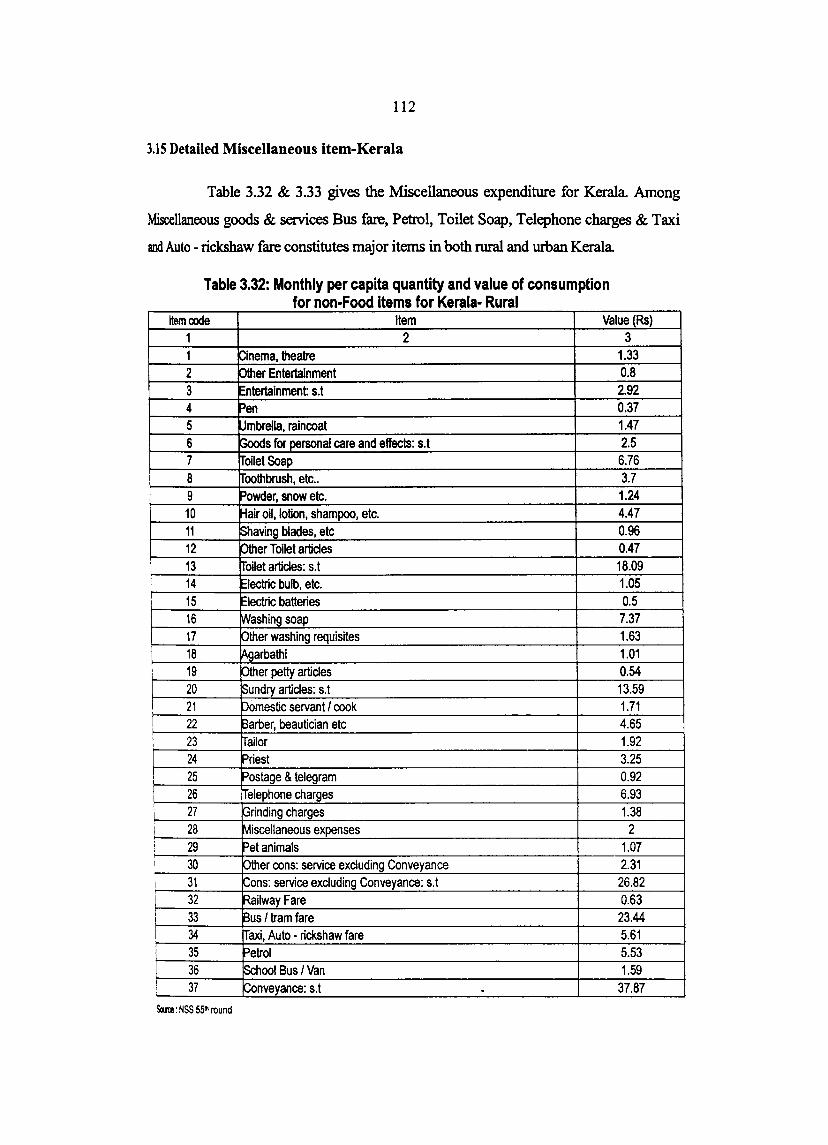
112
3.1S Detailed Miscellaneous item-Kerala
Table 3.32 & 3.33 gives the Miscellaneous expenditure for Kerala. Among
Miscellaneous goods & services Bus fare, Petrol, Toilet Soap, Telephone charges & Taxi
and Auto - rickshaw fare constitutes major items in both rural and urban Kerala
I
l I I i
I
;
Table 3.32: Monthly per ~apita quantity and value of consumption for non-Food Items for Kerala- Rural
Item code Item Value (Rs) 1 2 3 1 Cinema, theatre 1.33 2 Other Entertainment 0.8 3 Entertainment S.t 2.92 4 Pen 0.37 5 ~mbrella, raincoat 1.47 6 Poods for personal care and effects: S.t 2.5 7 ~oiletSoap 6.76 8 rroothbrush, ete .. 3.7 9 Powder, snow etc. 1.24 10 Hair oil, lotion, shampoo, etc. 4.47 11 Shaving blades, ete 0.96 12 ()ther Toilet articles 0.47 13 :r oilet articles: s. t 18.09 14 ~Iectric bulb, ete. 1.05 15 ~Iectric batteries 0.5 16 Washing soap 7.37 17 Pllier washing requisites 1.63 18 Agarbathi 1.01 19 Other petty articles 0.54 20 Sundry articles: s. t 13.59 21 Domestic servant I cook 1.71 22 Barber, beautician etc 4.65 23 rrailor 1.92 24 Priest 3.25 25 Postage & telegram 0.92 26 ~elephone charges 6.93 27 ~rinding charges 1.38 28 Miscellaneous expenses 2 29 Pet animals 1.07 30 Other cons: service excluding Conveyance 2.31 31 Cons: service excluding Conveyance: S.t 26.82 32 Railway Fare 0.63 33 aus I tram fare 23.44 34 ~axi, Auto - rickshaw fare 5.61 35 Petrol 5.53 36 ~ool Bus I Van 1.59 37 ~onveyance: S.t . 37.87
Sew : NSS 55111 round

113
Urban households spent Rs. 13.04 per capita on Petrol while it was only
Rs. 5.53 in rural sector. It is found that in rural as well as urban the expenditU!'e on
Miscellaneous items is very high as compared to the National pattern.
i
I
; ,
I
,
I
i
;
Table 3.33: Monthly per capita quantity and value of consumption -for Non-Food items for Kerala Urban.
Item code Item Value (Rs) 1 Cinema, theater 2 Vldeoetc 3 Entertainment s.t 4 es 5 Pen 6 Umbrella, rain coat 7 Goods for personal care and effects: s.t. 8 Toilet Soap 9 Tooth brush etc. 10 Powder, snow etc 11 Hair oil, lotion, shampoo etc. 12 Shaving blades etc 13 Sanitary items 14 Other Toilet articles 15 Toilet artides: s. t. 16 Elecbic bulb etc. 17 Bucket water boWe etc. 18 Washing soap 19 Other washing requisites 20 Agarbathi 21 Other petty articles 22 Sundry articles: S.t. 23 Domestic servant I cook 24 Sweeper 25 Barber, beautician etc. 26 Washer man, laundry 27 Tailor 28 Priest 29 Postage & telegram 30 Telephone charges 31 Repair charges for non-durables 32 Grinding charges 33 Miscellaneous expenses 34 Per animals 35 Other consumer services excluding Conveyance 36 Consumer services excluding Conveyance: S.t. 37 Railway Fare 38 Bus I train fare 39 Taxi, Auto - rickshaw fare 40 Petrol 41 Diesel 42 Lubricating oil 43 School BusNan 44 Conveyance: S.t
SMe:NSSO,551li ROUND S.l shows percentage
2.67 0.6 8.02 0.72 0.42 2.55 4.23 7.56 4.33 1.55 4.6 1.31 0.89 0.69 21.17 1.55 0.94 7.54 2.18 1.19 0.41 15.33 4.81 0.96 4.80 0.66 4.07 2.75 1.03 16.90 0.79 1.64 2.13 1.17 1.23
43.08 1.56
26.18 5.97 13.04 1.40 0.51 2.83
. 55.25

114
3.16 Educational & Medical Expenditure in India
Table 3.34: Monthly per Capita quantity and value of consumption for F d It b MPCE I f Alii d' I non· 00 ems )y c ass or n la rura.
, lIImoode Item Value [Rs.] I 1 2 4
1 Books, Journals 2.87
I 2 Stationery 1.51 3 Tuition and other fees 2.74
I 4 Private tutor I coaching centre 1.28 5 Other Educational expenses 0.69
I 6 Education: s1 9.37 7 Medicine 3.75
I 8 Doctor's I fee 0.78 I 9 Hospital charges 1.14 ;
10 Other Medical expenses 0.53 11 Medical· Institutional s.l 6.66 12 Medicine 19.11
I 13 X-ray, and other I tests 0.71 14 Doctor's fee 2.22 15 Other Medical expenses 0.87 16 Medical· non ·Institutional s.t 22.92
~.551M ROUND s.l shows sub total
Table 3.35 Monthly per Capita quantity and value of consumption for F d 't b MPCE I f Alii d' b non· 00 I ems ,y c ass or n la ur an.
; mcode Item Value[Rs.]
I 1 Books, Journals 6.87 ,
2 Newspapers, Periodicals 2.35 3
~
Stationery 3.05 4 uition and other fees 16.71 5 Private tutor I coaching centre 6.00 6 ~erEducationalexpenses 2.01 7 Fducation: s.t 37.05 8 ~edicine 5.78 9 X·ray, other tests 0.88 10 Doctor's fees 1.64 11 Hospital charges 2.86 12 Other Medical expenses 1.17 13 ~edical· Institutional S.t 12.33 14 ~icine 24.37 15 ~-ray, other tests 1.30 16 Poctor's 3.95 17 ~er Medical expenses 1.27 18 ~edical· non ·Institutional s.t . 30.95 ,
j,wtjSS(),551M ROUND s.l shows sub total

115
Households allocate a considerable amount per month on Educational and
M~cal expenses Per capita expenditure on Books / Iournals Periodicals, Tuitions
ifs Doctor's fees and medicine are shown in Table 3.34 and 3.35. It is found that
lI100g the non-Food items considered 'Medical non -institutional' constitutes the
~~est expenditure in rural fudia, and in urban fudia it is 'Education'
117 Education & Medical Expenditure Kerala
Per capita expenditure on Books, Iournals, Periodicals, tuition fees,
i)xtor's fees and medicine is shown in table's 3.36 & 3.37 It is found that the per
~itaexpenditure on Education is very high as compared to National pattern.
SI. No
1
2
3
4
5
6
7
8
9
10
11
12
13
14
15 I 16 i 17
18
Table 3.36: Monthly per capita quantity and value of consumption for non-Food items for Kerala.
Item Value (Rs)
Books, Journals 6.59
NewsDapers, Periodicals 7.61
~tationary 2.17
~uition and other fees) 8.79
Private tutor I coachina centre 6.63
tHherEducationalexpenses 2.9
Education: S.t. 34.73
Medicine 11.2
lX·ray, other tests etc. 2.35
poctor's 2.46
~osDital charges 9.51
Iother Medical expenses 1.84
Medical institutional: S.t 27.37
Medicine 33.2
lX·ray, other test etc. 3.11
poctor's 3.89
Iother Medical expenses 0.85
Medical- non- institutional: S.t 41.08 1 llIIt NSSO 55TH ROUND

116
Table 3.37: Monthly per capita quantity and value of consumption for Non-Food items for Kerala Urban.
9: No Item Value[Rs,] 1 aooks I Journals 4.44 2 ~ews papers, Periodicals 4.32 3 ~tationary 1.87 4 ~uition and other fees etc 4.86 5 Private tutorl coaching centre 3.25 6 Pther Educational expenses 1.4 7 ~ducation: s.t 20.16 8 ~icine 10.22 9 ~-ray, other test etc 2.07 10 Doctor's 1.81 11 ~spital charges 5.23 12 Other Medical expenses 2.23 13 Medical- institutional: s.t 21.56 14 Medicine 32.9 15 X-ray other tests ete 1.97 16 Doctor's 3.47 17 Other Medical expenses 0.92 18 Medical- non-institutional: s.t 39.27
_ NSSO 55' round
Among Education and Medical expenses, tuition fees and medicines
_lUte major items in both rural and urban sectors. Per capita expenditure on
:.ducation amounted to Rs. 20.16 in rural and Rs. 34.73 in the urban.
H8 Consumption level and pattern of different fractile groups
Differences in consumption pattern of poorer and richer segments of
~ation (ranked by MPCE) have been attempted using approximate fractile of the
ll?CE distribution as class limits. Table 3.38and 3.39 gives the item - group wise
~Jk·up of average MPCE for twelve fractile groups of MPCE for all India starting
~ the bottom 5% and ending with top 5%.
In the rural sector the average MPCE of the bottom 5% was around Rs. 120
r l3S in Kerala and at the all-India level it was Rs. 101 in the urban sector the
il-erage MPCE OF the bottom 5% was Rs. 133 for the country as a whole and it was
hl47 for Kerala.

117
Table 3.38: Value (Rs) of consumption of broad groups of Food & non-Food items per person of 30 days for each fractile group. All-India
Rural Fractile group
Item 0-5 5-10110-20 20-30 ~ 40-50 50-60 60-70 70-80 80-90 90-95 ~5-10C , !Heals 40.9 51.96 57.9 62.51 ~7.12 68.42 71.2 73.36 ~5.82 76.13 ~9.07 85.83
i(m 0.09 0.16 0.17 0.26 0.34 0.42 0.54 0.55 0.72 0.92 1.14 1.68
l ~subsl 0.1 0.11 0.1 0.13 0.17 0.24 0.22 0.3 0.37 0.51 0.54 0.74
, p.s&prod. 5.17 6.38 7.29 8.27 8.89 9.92 10.6 11.45 12.64 14.01 16.2B 20.54
i .&prod. 2.42 4.79 7.29 10.52 13.74 18.16 23 28.37 36.54 49.26 65.42 87.86
~~oiI 5.22 6.69 7.81 9.01 10.07 11.2 12.4 13.54 14.94 17.14 18.8 25.69
all
68.1
0.54
0.28
10.7
26.7
12.4
1 Neat. Eggs. Fish 2.04 3.08 4.35 5.55 6.79 7.79 9.14 10.27 11.87 1 iI /;,:: 17.01 24.51 9.37 .,."'''"'
I~ 7.8 10.01 11.6 13.17 14.56 15.6 17.3 18.66 ~0.09 22.47 ~5.02 30.48 17
S FniIs (fresh) 0.56 0.88 1.19 1.57 2.01 2.64 3.11 4.05 5.1 7.25 9.83 15.71 ~.04 ID FniIs (my) 0.24 0.2 0.31 0.39 0.43 0.58 0.65 0.77 0.98 1.33 1.98 3.6 0.85
t1&~ 2.77 3.55 4.36 5.32 6.1 7.15 8.11 9.29 1C,66 13.12 15.39 21.43 8.57
12 Sal 0.38 0.41 0.45 0.47 0.49 0.5 0.53 0.53 0.57 0.59 0.62 0.73 ~.52 13~ 3.55 4.22 4.78 5.43 5.9 6.39 6.92 7.33 8.1 8.98 10.05 12.66 6.91
14 Mages, refreshments ete 2.7 3.6 4.92 6.19 7.21 8.63 10.2 11.98 14.3a 18.74 23.36 39.59 11.7
15 Food~ 73.9 ~.11 113 128.8 143.8 157.6 174 190.4 212.B 245 284.5 371.1 178
11 PIl, Tobacco & intoxicants 3.78 4.7 5.49 6.26 7.04 7.83 8.73 9.55 10.87 12.14 13.96 21.1 8.97
!7 ueI& Ight 11 13 14.4 15.67 17.05 18.52 20 21.45 23.5 26.96 29.91 44.81 20.7
!e~ 0.92 1.42 2.17 2.98 4.19 5.79 7.92 10.85 16 27.02 ~7.49 98.73 15.1
'9fcdwear 0.26 0.24 0.41 0.67 0.78 1.09 1.47 2 2.8 4.53 7.61 13.94 2.48
'J /.isc. good & services 11.1 15.0B 18.3 22.64 ~6.34 31.46 36.4 44.44 ~.52 72.62 104.5 230.2 ~8.7 ~~goods 0.37 0.63 0.78 1.17 1.54 1.94 2.48 3.64 4.1 7.29 11.08 95.53 7.67
:1 tbrFood; total 27.4 ~5.01 41.5 49.39 56.93 66.63 77 91.94 111.8 150.6 214.5 504.3 104
Zl ~oIaI expenditure (Rs.) 101 13U 154 178.2 200.8 224.3 251 282.4 324.6 395.6 499 875.3 281 _ NSSO 50" round
Average monthly spending levels of the top 5% of the population varied
:"1IISiderably in the rural sector. For Punjab, Haryana and Kerala-the three states with
tighest average rural MPCE for the whole population it was Rs. 13001-. For India as a
-hole the average MPCE OF the top 5% ofthe population was Rs. 875.
In the urban sector there was inter state variation in average spending of
:c lOp 5% average MPCE of the top 5%. Of the all-India population was Rs. 1626.
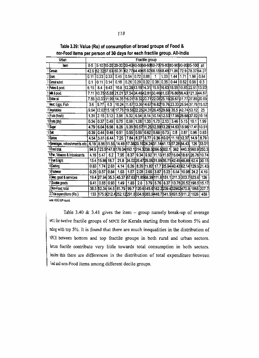
118
Table 3.39: Value (Rs) of consumption of broad groups of Food & non-Food items per person of 30 days for each fractile group. All-India
Urban Fractile group Item 0-5 5-10 10-20 20-30 ~o O-!\I' ~n R0-7 70-8 80-90 0-9 5-100 all
1 C«eIs 42.6 52.3</ ~7.63 60.31 2.77 ~.4 5.92 68.15 8.4 71.86 72.9 78.37 64.27 1 Gram 0.11 0.23 0.33 0.45 0.54 0.72 0.88 1 1.03 1.44 1.71 1.98 0.84 l Cereal subst 0.1 0.11 0.14 0.18 0.26 0.29 0.32 0.38 0.35 0.44 0.52 0.56 0.3 4 Pulses & prod. 6.15 8.4 9.43 10.8 12.2S 13.1 14.31 15.5 16.6~ 18.55 19.8 22.61 13.92 5 1&& prod. 7.11 10.75 15.6S 21.01 7.54 34.4 42.81 50.4 1.0 76.86 8.4~ 121.3 ~.87 6 _oil 7.56 10.0.: 11.99 14.35 16.01 18.32 20.71 22.0 5.1 28.67 31.77 37.89 20.09 : tJieat, Eggs, Fish 3.6 5.77 8.3 10.24 11.67 13.3 14.67 16.8.0/ 19.7 23.33 ~6.94 37.76 15.52 8 ~tabIes 9.64 12.6~ 15.18 17.76 19.58 22.2 24.31 26.45 29.8 35.5 142.74 53.12 25 ~ ruils (fresh) 1.31 2.15 3.12 3.96 5.32 6.54 8.14 10.14 12.5 17.98 26.6 37.92 10.18 10 ruits (dry) 0.34 0.37 0.49 0.75 0.98 1.08 1.33 1.73 2.13 3.46 5.15 10.1 1.99 11 Sugar 4.79 6.04 6.98 8.26 9.39 10.57 11.25 12.5 13.2 14.63 15.9S 17.41 10.91 12 ~ 0.39 0.44 0.48 0.51 0.55 0.59 0.62 0.68 0.73 0.8 0.87 0.96 0.63 13p 4.54 5.61 6.44 7.25 7.84 8.27 8.n 9.36 10.01 11.18 12.37 14.9 8.79 14 ~,refreshments ete .6.19 8.96 11.56 14.49 17.311 20.1 ~4.24 31.1~ ~1.1 57.28 84.4 126 33.01 15 GOd kltal 94.5 123.~ 147.E 170.~ 192.1 ~14.~ 238. ~66. 302. 1 362 1440.3 560.9 250.3 16 PI\, Tobacco & intoxicants 4.16 5.47 6.2 7.95 8.37 9.34 9.92 11.13 11.9 715.04 18.6 126.76 10.74 17 ueI & light 13.4 15.9 18.7 21.8 ~4.0 26.4 ~.O 31.00 ~.7 142.45 48.8 62.4 30.15 \8~ 0.83 1.74 2.63 4.14 6.26 8.26 11.82 17.7 ~5.94 40.43 62.1 4129.5 21.4 19 ootwear 0.26 0.57 0.84 1.03 1.57 2.08 2.65 3.87 5.23 6.64 10.9 824.2 4.19 Z! ~. good & services 19.4 27.94 35.3 45.37 ~7.6 171.8 ~8.3 111.8 151. 1211.3 ~03. 7623.6 126 ~~goods 9.41 0.65 0.93 1.49 1.85 2.6 3.79 5.76 8.37 13.78 ~6.5 198.5 15.17 12 ~ood; total 38.5 ~2.~ 64.6 81.79 99.7 120. 145. 182. 239.4 ~296j/ 1470. 91065 207.7 13 DIal expenditure (Rs.) 133 175. 212. 4252.1~ 291. 334. ~83. 1448. 541. 691.5 911. 21626 458 iw. NSSO 50" round
Table 3.40 & 3.41 gives the item - group namely break-up of average
IIPCE for twelve fractile groups of MPCE for Kerala starting from the bottom 5% and
:lIiing with top 5%. It is found that there are much inequalities in the distribution of
\!PCE between bottom and top fractile groups in both rural and urban sectors.
3onom fractile contribute very little towards total consumption in both sectors.
3c:sides this there are differences in the distribution of total expenditure between
~ood and non-Food items among different decile groups.

119
Table 3.40 Value (Rs) of consumption of broad groups of Food & non-Food items per person of 30 days for each fractile group Kerala • Rural
Fractile group
Item
Kerala
· t Cereals 38.3 48.3657.8559.83~.2366.0571.84~2.8576.03 82.3684.1995.6868.45
2 Gram 0.17 0.58 0.38 0.64 0.75 0.88 1.06 1.26 1.48 1.35 2.04 2.83 1.06
3 Cereal subsl 2.89 1.87 3.19 3.89 3.26 4.52 4.47 4.96 5.37 5.31 5.59 3.46 4.19
4 Pulses & prod. 1.35 3.17 3.46 5.05 5.53 6.29 7.9 7.94 9.02 10.2912.36 16.18 7.2
i 5 fa&prod. 2.4 4.37 7.57 7.36 10.5614.1418.86 25.2 ~.08 32.49 ~1.42 58.95 ~0.3~
6 EdiJIe 011 5.38 6.1 7.04 8.44 9.4 10.14 11.4212.45 12.91 14.65 18.62 23.03 11.3
7 Meat, Fish & Eggs 12.415.0/17.7220.53~3.0/~7.3~ 31.03;36.54 41.8 49.1557.57 80.56 33.01
I 8 ~lIes 6.7 8.37 9.47 11.3912.9~ 13.91 17 17.7619.58 22.5 26.9B 34.09 16.27
i 9 ruits (fresh) 5.65 9.07 11.3714.3517.3~ 19.74 23.63 ~.13 29.36 34.2 44.8 53.96 23.29 I
I 10 ruits (dry) 0.04 0.09 0.15 0.23 0.2 0.31 0.45 0.48 0.53 1.16 1.62 3.4 0.61
." Sugar 4.12 6.11 7.16 8.04 8.69 9.1 9.94 11.3111.47 12.6 14.54 17.72 9.96
1,2 SIt 0.28 0.34 0.35 0.37 0.4 0.42 0.47 0.49 0.51 0.56 0.65 0.73 0.46
13 Spires 5.27 6.18 7.35 8.45 9.07 9.56 10.6~ 11.3111.59 13.02 14.83 16.02 10.2~
14 Beverag~, refreshments etc. 7.97 13.2415.2720.7523.4327.4628.8629.4433.47 42.82 ~6.47 81.33 ~9.62
IS oodtotal(1-14) 92.9122.~ 148.3169.3188.8~09.9237.6258.~ 282.2322.46381.7~87.94 236
IS Pan, Tobacco & intoxicants 4.87 7.19 6.67 8.78 11.5714.9413.02 13.4 15.58 19.5920.73 20.31 13.01
17 uel & light 11.9 14.7 14.9B 16.5919.5221.1222.2B~3.5625.45 29.3236.9938.8522.41
18 CIo1hing 0.82 0.3& 1.79 3.31 5.73 6.77 5.3 9.89 18.61 37.61 56.82 99.49 16.8
19 ootwear 0.41 0.24 0.69 1.24 1.39 1.85 2.93 3.65 4.66 6.69 6.73 17.14 3.54 I · 20 Mise. good & services * 18.8 25.3S 32.5141.38 47.7 ~3.09 ~9.74 77.77~3.14115.53169.1 311.82~8.3~
2t Durable goods - 1.21 0.6 0.59 0.72 1.41 2.91 1.76 2.99 12.84 30.48324.38~0.23
22 Non·Food total 36.74 49.1157.24 71.89~6.62 ~9.1S 106.2 130 160.5221.5/320.9812.01154.4
• 23 otal expenditure (Rs.) 130 172 ~05.6 241.2~75.~ 309.1343.8 388.2~2.7544.0~~02.6 1300 ~90.4
SMe: NSSO 5Q1h round

120
Tabl,3.41 Value (Rs) of consumption of broad groups of Food & non.food items per person of 30 days for each fractile group. Kerala • Urban
Item 0-5 5-10 10:- 20- 30- 40- 50- 60- 70- 80-90 90- 95-20 30 40 50 60 70 80 95 100 .
Keria I No. of sample blocks: 183 .~ 39.6 49.15 53.3 60.34 58.47 64.76 70.24 69.07 71.35 72 77.3 77.31 : !CGn 0.6 1.02 0.82 1.06 1.02 1.24 1.43 2.04 1.59 2.38 2.96 3.25 ~ !CreaI subsl 1.54 1.96 2.42 1.52 1.79 2.09 2.34 1.79 1.42 1.68 2.16 1.52 ~ jNses & prod. 2.03 2.97 4.47 5.24 6.32 7.59 7.22 9.53 10.55 11.67 14.03 17.09 : JIil & prod. 4.82 9.24 11.21 12.66 17.01 23.12 23.61 30.49 34.06 44.22 64.77 81.22 E~oiI 5.65 7.21 8.5 10.43 10.1 11.51 12.07 14.29 15.48 17.03 19.56 23.46 • Yet Eggs, Fish 13.06 22.48 21.6 25.74 30.96 32.31 39.16 46.47 46.58 509.13 77.5· 83.12
a~ 6.58 7.56 10.18 11.68 12.46 15.16 15.55 19.43 19.89 23.54 32.13 36.03 S fnits (fresh) 8.95 11.92 14.67 17.88 19.23 23.21 25.68 29.08 30.81 37.77 53.1 57.66 ~FniIs (dry) . 0.08 0.07 0.13 0.23 0.69 0.43 0.86 0.43 1.33 2.84 4.12 . ~~ 5.44 6.86 7.68 8.95 9.59 10.19 10.54 10.95 12.59 14.04 16.83 18.16
'~~ 0.33 0.39 0.4 0.44 0.45 0.49 0.5 0.51 0.67 0.58 0.72 0.78 "~ 5.17 6.19 7.59 8.44 9.15 10.09 10.56 10.55 11.39 12.25 13.61 14.39 .~~, ~tsetc. 11.1 16.94 17.3 27.02 36.2 34.35 34.24 38.87 52.35 70.75 95.29 148.9
1~~kJIaI 104.9 143.96 160.2 191.5 213 236.8 253.6 284 309.2 368.4 472.8 567 I~P., Tobacco & ~ts
3.77 5.67 6.72 9.17 9.73 11.28 16.41 16.65 10.63 14.44 11.93 26.31
, ~&ighl 13.46 16.11 17.88 21.7 23.37 24.58 25.76 28.48 33.14 35.91 44.14 51.89 1~ 2.49 0.75 7.15 6.24 10.16 16.07 19.92 32.41 42.26 80.05 79.88 211.1 'hIwear 0.44 0.8 1.23 1.45 1.75 3.54 2.58 4.17 5.9 8.48 12.27 24.43
~~&serkes* 22.31 30.04 42.34 51.08 60.39 67.11 85.24 98.43 142.4 175.9 292 658.7 ~'-goods . 0.26 0.81 2.39 1.05 2.5 5.2 2.06 9.14 16.88 14.29 396.5 :2Wood total 42.45 53.63 76.13 92.02 106.4 125.1 155.1 182.2 243.5 331.7 454.5 1369 :l~WI expenditure (Rs.) 147.3 197.59 236.4 283.6 319.4 361.9 408.7 466.2 552.7 700.1 927.3 1936 :.w: NSSO 5()Ih round
All
64.13 1.55 1.86 8.07 27.67 12.74 40.04 16.92 25.43 0.77 10.82 0.52 9.97
44.77
266.3
11.9
27.08 36.21 4.81 122.6 24.64 227.6 493.8
l.19 Trends in an rage consumption expenditure and in consumption pattern
over the last two decades in India
The composition of household MPCE at all-India level is shown for the
5:xcessive consumer expenditure surveys ofNSS in tables 3.42 &3.43.
Apart from absolute values of average MPCE, the bottom of the table
(:aent indices of average MPCE using the 1972-73 figures as base. The corresponding
:oosumer price indices (CPI for agriCUltural workers for rural areas and CPI for non
:wIuaI employees for urban areas) again with 1972-73 as the base are SRown in the
~ row of the table.25

121
Table 3.42: Value of consumption of broad groups of items per person
for a period of 30 days by NSS rounds India Rural Item Oct·72· Sep-73 ul·77.Jun·7E an-dec83 ul-87.Jun·88 ul·93-Jun·94 ul·99-jun·2000
CM ~
rmsOOsl ~&prod.
11 & 1IOd. ~o1 • Eggs, FISh . .. kG & ools r;q;------S.&spces _etc. foldlli
PI. lam & intoxicants hII&ij11 --1& LIJOd & services • Ddagoods afoIxI kIIaI .upnlilure (Rs.) tFCEi1dex \2lII round = 1 (0) r.mer Price index jV'II round = 1 (0) ~j~ VlIIOUS round '!IcIudcs rents and Taxes
17.92 0.25 0.24 1.89 3.22 1.55 1.09 1.59 0.45 1.66 1.23 1.07 32.16 1.36 2.49 3.09 0.23 3.89 0.95 12.01 44.17
100
100
22.59 0.29 0.23 2.63 5.29 2.46 1.84 2.6
0.77 1.82 2.09 1.72
44.33 1.99 4.13 5.99 0.51 7.12 4.82 24.56 68.89
156
144
36.21 41.33 0.29 0.38 0.21 0.21 3.98 6.27 8.5 13.63 4.53 7.88 3.37 5.11 5.31 . 8.23 1.54 2.57 3.18 4.51 2.82 4.52 3.69 6.18 73.63 100.8 3.35 5.03 7.92 11.77 9.64 10.52 1.11 1.55
14.06 22.78 2.6 5.64
38.68 57.28 112.3 158.1
255 358
227 289
Tbefollowing are among the noticeable features of the data.
68.1 107.8 0.5 0.64 0.3 0.36 10.7 18.5 26.7 42.56 12.5 18.16 9.4 16.14 17 29.98 4.9 8.36 8.6 11.57 7.4 14.41 11.7 20.38
177.8 288.8 8.9 13.96 20.7 36.56 15.1 33.28 2.5 5.37 48.7 95.43 7.7 12.76
103.6 197.4 281.4 486.2
637 1100
520 833
a) The rural MPCE at all India level has risen fonn Rs. 44 in the 72·73 to Rs. 486
in the 99·2000. The corresponding estimates for per capita expenditure on
Food has increased from Rs. 32 to Rs. 289 and per capita expenditure on non·
Food has increased from Rs. 12 to Rs. 197.
b) The urban MPCE at all-India level has risen from Rs. 63 in the 2th round to
Rs. 855 in the 55th round. The corresponding estimates for per capita
expenditure on Food has increased from Rs.41 to Rs. 411 and per capita
expenditure on non-Food has increased from Rs. 22 to Rs.444.

122
TIbIe 3.43 Value of consumption of broad groups of items per person for a period of 30
Item
ems Inn Rlsubsl pJses & prod. .& prod. E!jeoo
,.. Eggs, Fish
~ film & nuts .. 6il&spces a..setc. Fo:xIkIIaI
PI!, TOOI:co & intoxicants ht&1ght 0ti1g futa .. good & services * tnMgoods Imfoodtotal bIIupendilure (Rs.) lFCEiIdex
Wltroond = 100) CaIuner Price index j21I1roond = 100) iwI: NSS Various rounds ... rents and Taxes
d b NSS did' ays ,y roun s n la. . InRs .
pct-72-Sep-73 ul-77-Jun-78 an-DeC'r83 u1-87 -Jun-88 14.77 19.66 31.85 36.97 0.20 0.24 0.31 0.41 0.08 0.10 0.13 0.17 2.16 3.43 5.32 8.44 5.91 9.16 15.27 23.84 3.07 4.46 7.98 13.23 2.07 3.33 5.93 8.85 2.77 4.23 8.17 13.12 1.27 1.66 3.413 Po ?7
2.28 2.54 4.06 5.86 1.44 2.55 3.55 5.78 4.82 6.09 11.26 16.82 40.84 57.67 97.31 139.7 1.75 2.34 4.05 6.53 3.57. 6.17 11.40 16.72 3.34 6.78 12.80 15.00 0.26 0.59 1.84 2.69 12.17 14.05 33.85 58.64 1.40 8.55 4.55 10.60 22.49 38.48 68.49 110.2 63.33 96.15 165.80 249.9
100 152 259 395
100 160 258 364
Urban ul-93-Jun-94 ul-99-Jun-200C
64.3 105.57 0.80 0.95 0.30 0.35 13.90 24.25 '. 44.90 74.17 20.10 26.81 15.50 26.78 ' 25.00 43.90 .' 1? ?n 20.68 _._-
10.9 14.00 9.40 19.11 33 54.28
250.3 410.84 10.70· 16.22 30.20 66.26 21.40 51.76 4.20 10.05
126.00 232.62 15.20 30.85 207.7 444.08 458.00 854.92
724 1351
618 998
c) The share of Cereals in household consumer expenditure has fallen steadily in
both rural and urban areas. In rural areas it has fallen from 41 % to 22% and in
urban areas from 23% to 12%.
d) In the rural sector the share of Food as a whole has also substantially decline
since the 2th round (1972-73). The share of some Food groups, notably Milk
and Milk products, Vegetables and Beverages, refreshments and processed
Food has increased in this sector at the expense of the share of Cereals.
e) In the urban sector, the share of Food has continued to fall throughout the
period 1972-1999, the over all decline being of order of 16 % points. In this
sector the shares of the Non-Cereal Food groups have not changed much. A fall
in the share of Sugar from its 27th round value is the only noticeable change.26

123
o Among non-Food groups, the category Miscellaneous goods & services
registered a steady rise in share over the period under consideration. In the
rural sector the share of this category has increased from 36% to 52%.
g) Both in rural and urban areas the overall rise in MPCE over this period was a
little higher than the rise in consumer prices between 1972-73 and 1993.:.94.
Table 3.44 &3.45 give the % composition of household MPCE.
Table 3,44: Percentage distribution of MPCE by 18 groups of
Item
CnaIs
rm !'nil subsl
Pes & prod.
IIllWOd·
Ei*oI IIei, Eggs, Fish
~ f1IiIs l nuts
• Sill Spices
Nagesetc.
Fo:dbtal
~, Tobacco & intoxicants
FiIJ&light
Q.Ug
F~r
Ibc. good & services *
~goods
~oodtotal
"da expenditure (Rs,)
iw: NSS Various rounds
'IQIIes ranls and Taxes
" 'I d' consumption Items In n la InRs.
Oct-72-Sep-73 ~ul-77 -Jun-78 ~; _n-Jl'l an-_v v Ilul-87 -Jun-8B
40.6 32.8 32.3 26.3
0.6 0.4 0.3 0.2
0.5 0 .. 3 0.2 0.1
4.3 3.8 3.5 4.0
7.3 7.7 7.5 8.6
3.5 3.6 4.0 5.0
2.5 2.7 3.0 3.3
3.6 3.8 4.7 5.2
1.1 1.1 1.4 1.6
3.8 2.6 2.8 2.9
2.8 3 2.5 2.9
2.4 2.5 3.3 3.9
72.9 64.3 65.6 64
3.1 2.9 3 3.2
5.6 6.0 7.0 7.5
7.0 8.7 8.6 6.7
0.5 0.7 1.0 1.0
8.7 10.3 12.5 14.5
2.2 7.0 2.3 3.1
27.1 35.7 34.4 36
100 100 100 100
~uI-93-Jun-94
24.2
,0.2
0.1
3.8
9.5
4.4
3.3
6.0
1.7
3.1
2.7
4.2
63.2
3.2
7.4
5.4
0.9
17.3
2.7
36.8
100
Rural
Jul-99-Jun-2000
22.2
0.1
0.1
3.8
8.8
3.7
3.3
6.2
1.7
2.4
3.0
4.2
59.4
2.9
7.5
6.9
1.1
19.6
2.6
40.6
100

124
T bI 345 P d' t 'b f f MPCE NSS d a e • . ercentage IS rl U Ion 0 over roun 5 . tnRs.
hem Pct-72-Sep-7~ ~ul-n- Jun-7B Jan-Dec-8~ ~u1-87 -Jun-8B ~ul-93-Jun-94 .
Ceeiis
Cm
CNsubsl p Jses & prod.
MUIJOd· fjE(j
"Eggs,Fish
~ FW&nuts .-SiI&Sji:es
&.agesetc. F«dmlal PI!. TacxxI & intoxicants
ht&ItJII DfiIg
Fa. IIK,ad & services • IUiEpds
~total
"daI expenditure (Rs.) _ NSS Various rounds
'IaIis III1IS and Taxes
2 3 23.3 20.5 0.3 0.3 0.1 0.1 3.4 3.6 9.3 9.5 4.9 4.6 3.3 3.5 AA 4.4
2.0 2.0 3.6 2.6 2.3 2.7 7.6 6.3 64.5 60 2.8 2.4 5.6 6.4 5.3 7.1 0.4 0.6 19.2 14.6 2.2 8.9 35.5 40 100 100
4 5 6 19.4 15 14 0.2 0.2 0.2 0.1 0.1 0.1 3.2 3.4 3.0 9.2 9.5 9.8 4.8 5.3 4.4
3.~ 3.6 3.4 5.0 5.3 5.5 2.1 2.5 2.7 2.5 2.4 2.4 2.1 2.3 2.0 6.8 6.8 7.2 59.1 56.4 54.7 2.4 2.6 2.3 6.9 6.8 6.6 7.6 5.9 4.7 1.1 1.1 0.9
20.5 23.2 27.5 2.3 4.1 3.3 40.9 43.6 45.3 100 100 100
Urban
ul-99-Jun-2000 7
12.4 0.1 0.0 2.8 8.7 3.1 3.1 5.1 2.4 1.6 2.2 6.4
48.1 1.9 7.8 6.1 1.2 27.2 3.6 51.9 100
JlO Trends in average consumption expenditure and in consumption pattern
over the last three decades in Kerala
a) The rural MPCE of Kerala has risen from Rs. 42 in the 27th round to Rs. 765 in
55 th round. (The corresponding estimate for per capita expenditure on Food
has increased from 29 to Rs. 411 and for per Capita expenditure on Non-Food
has increased from Rs.12 to Rs. 354.)
b) The urban MPCE of Kerala has risen from Rs. 58 in the 2th round to Rs. 932 in
the 55th round. (The corresponding estimate for per capita expenditure on
Food has increased from Rs. 37 to Rs. 457 and for per capita expenditure on
non-Food h~ increased from Rs. 20 to Rs. 475.)

125
cl The share of Cereals in household consumer expenditure has fallen steadily"in
both rural and urban areas. In rural areas it has fallen from 32% to 14% and in
urban areas from 24% to 11 %.
di In the rural sector the share of Food as a whole has also substantially declined
since the 2th round. The share of some Food groups, notably Milk and Milk
products. Meat, Eggs and Fish, Fruits & nuts Vegetables, Beverages,
refreshments and processed Food have increased in this sector at the expense
of the share of Cereals.
=.1 In the wban sector the share of Food has continued to fall through out the period
1972 -1999. The over all decline being of the order of 17% points. In. this sector
the shares of the Non-Cereal Food groups have not changed much. A fall in the
share of Sugar from its 27th round value is the only noticeable change.
o Among non-Food groups the category Miscellaneous goods & ServICes
registered a steady rise in share over their period 1972-1999. In. the rural sect.or
the share of this category has increased from 45% to 51 %. This category has
registered a decline in share over the period 1994-1999. In. the rural and urban
sectors of Kerala as different from the trend observed earlier the share of Non
Food has continued to rise through out the period 1972-99 from 29.58% to
46.30% in the rural and from 35.14% to 51 % in the urban sector.
51 Both in the rural and urban areas, the overall rise in MPCE over this period were
a little higher than the rise in consumer prices between 72-73 and 99-2000.
i21 Possession of Durable goods
Household consumer goods other than Food, Fuel and Clothing /
=XlWear are according to usual NSS practice classified into Durable.goods.and-a
lSldual Miscellaneous goods category. Durable goods are distinguished from
~JCellaneous goods by having a longer expected lifetime of use (roughly, one year
I more). Durable goods used for household purposes thus include Furniture and
_. recreational goods such as cameras, TV, Cassettes and musical instruments,
f.felry and ornaments clocks and watches, household utensils and appliances for
:ding, heating, cooling and other work such as sewing, vehicles' for personal
:msport and other electrical and sanitary fittings.

126
Expenditure on durables, for the population as whole, forms a very small
~on of total household expenditure. Per capita household expenditure on
_Ies in 1999-2000 was estimated as Rs. 12.76, (2.6% of total household
:tpenditure) in rural areas and Rs. 30.85 (3.60%) in urban areas of the country. Per
~ita household expenditure on durables in Kerala was Rs.52.51 (6.81) and Rs.
~3.~ ,6,8%) in urban Kerala.
Expenditure incurred on repairs and construction of' d~rables used for
ixnestic purpose is included in expenditure on Durable goods: The all deciles groups
5gures for certain important items are considered first. % of rural and urban
11useholds reporting possession of fourteen important household durables in India
lid Kerala are shown in Table 3.46.
9-lit , , j
,
j
: . !
1
'l 'I
'l 'l
'4 I~
'i
" ,
'!
": ~
~ "
11
1l
Table 3.46 Proportion of households possessing different Items of Durable goods (Number per 1000)
Item All-India
Rural Urban Rural Bedstead 791 818 873 Almirah, Dressing table 269 561 587 Chair, stool, bench, table 529 741 931 Suitcase, and other Travel goods 737 827 557 Foam, rubber ete 24 125 118 Carpet & other floor matting 153 227 40 Paintings etc, 19 78 10 record player etc 6 17 17 Radio 304 351 495 Television 187 595 338 VCRJVCP 5 37 65 Tape recorder, CD player 91 278 333 Electric fan 263 685 487 />jr conditioner r etc 17 109 3 Sewing machine 74 203 115 Washing machine 6 89 35 Stove 273 618 380 Pressure Cooker 131 496 195 Refrigerator 27 229 138 Bicycle 405 390 195 Motor cycle I Scooter 45 184 65 Motor car, jeep 4 27 20 CIock,watch 389 604. 803
iw: NSS 551h round
Kerala Urban 906 729 927 669 226 86 19 17
434 568 138 402 718 10 195 108 599 368 284 249 141 40 819

127
The % of possessor households in urban areas are in nearly all cases higher
Ihan the corresponding % for rural areas. Rural- urban differences in incidence of
possession are seen to be low in case of bedsteads (79% for rural India and 81 % for
Ulban India) and also low for bicycles (40% for rural and 39% for urban).
For all the other durables listed in the table rural-urban differentials were
much higher. Examples are TV I VCR / VCP and pressure cooker (rural 13%, urban
49%) Electric fan (rural 26%, Urban 68%) and refrigerator (rural 2%, Urban 22%).
Rural - Urban differentials were somewhat less marked tor ra<1lOS an<1
clocks / watches both of which were possessed by more the quarter of all rural
households in 99-00.
The % ef possessor households in urban areas are in nearly all cases
bigher than the corresponding % for rural areas. Rural - urban differences in
incidence of possession are seen to be low in case of bedsteads (87% for rural, 90%
for urban).
For all the other durables listed in the table rural urban differentials were
much higher examples are electric fan (48% for rural, 71% for urban) and stove (38%
for rural, 59% for urban). Rural -urban differentials were somewhat less marked for
radio and clocks / watches.
Regarding possession of Durable goods there is much difference observed
between households in National level and those in Kerala. Items with wider
differences in possession are explained here.
3.21.1 Entertainment items:
3.21.1.1 Radio, TV and Tape recorder
Radio sets were possessed by 50% of rural households in Kerala and 30%
of rural households in India. Tape recorders and CD players were present in 33% of
rural households in Kerala. This was only 9% for rural Indian households. In urban
areas of Kerala the incidence was 40.44% and the same 27% in All India urban.
128
The % of rural households reporting possession of VCR / VCP are seen to
x6%forKerala while it is less than 1% for all major states. In urban areas ofKerala,
:~lofhouseholds possessed VCR I VCP.
In rural areas, the proportion of households possessing television is 34%
~Kerala while it is only 18% of all India rural level.
Ui.2 Equi~ment for housework: Refrigerators, washing machines, pressure
cookers, stoves and sewing machines.
It is found that only 3% of rural households and 23% of urban households
in India were found to possess a refrigerator. The proportion of rural households
lving pressure cooker in Kerala was 14% and for all India it was 13%. As far as
mban sector is concerned the proportion becomes 36% and 44% respectively.
The use of washing machines was found to be 15 times more frequent in
mban India compared to rural India. The proportion of rural households having
i1Shingmachines in Kerala was 3% while the same was 10% in urban Kerala.
About 38-40 % of rural households possessed stoves in Kerala while it
(as 27% at the National level. In urban Kerala the proportion of households having
stoves was 60% at all India level.
3.21.3 Personal Transport equipments:
3.21.3.1 Motor cycles, Scooters and Bicycles
Kerala had the lowest proportion (20%) of rural households possessing
bicycles. The proportion was 40% in rural India. In urban Kerala only 24% of
households possessed bicycles while it was 39% in urban India. Interestingly the
proportion was much lower in urban areas, no doubt due to the widespread use of
motorcycles and scooters in preference to bicycles.
The %. of households with motorcycles / scooters was around 18% in
urban India and 5% in rural India. The incidence was 18% in urban and 6% in rural
Kerala.

129
J.l1.4 Comfort goods
lll.4.1 Air coolers I conditioners and electric fans.
The % of rural households with electric fan in rural India was 26% while
that was around 68% in urban India. In urban Kerala 71% households possessed
electric fans while in the rural areas the incidence of possession was 48% only. Air
coolers / conditioners were present in 11 % of urban households in the country as a " .
whole and 10% of urban households in Kerala. In rural Kerala the possession of the
commodity was reported by 3% of households.
3.21.5 Other durables
In both rural and urban areas around 80% of households possessed
bedsteads in all India. Both rural and urban areas of Kerala had around 80%
households possessing clocks / watches. While in urban India 2% of households
reported possession of motorcar, jeep, in urban Kerala it was 4%.
3.ll Average Number of Durable goods possessed by households reporting possession
Table 3.47 shows for each of23 different Durable goods, average number
possessed by 1000 households in rural and urban areas of Kerala and all-India. The
following features deserves mention.
3.22.1 Furniture
Bedstead is the only item out of the 23 items under consideration, for
which the average number of bedsteads possessed by a rural household '{2.5) is more
than that in urban areas (2.1). The average number is more or less the same in the two
sectors for bicycle (0.4). For all the other items the average number was less in rural
compared to urban.
In Kerala the proportion of households owning bedsteads "is somewhat
same in both rural (2.1) and urban (2.3). The average number of almarah, dressing
table & chair possessed by households in rural Kerala are lesser than urban
households.

130
Table 3.47 Average Number possessed per 1000 households
Sltl. Item Rural Urban
Kerala All-India Kerala All-India 1 Bedstead 2159 2474 2372 2117 2 Almirah, dressing table 917 388 1242 935 l Ch;lir, tab le ete 5452 1567 6367 2923 4 Suitcase, and other, Travel goods 1057 1896 1508 2629 5 Foam, rubber 251 55 556 371 6 Carpet, and other floor matting s 69 382 157 523 7 Painting, ete 18 49 48 204 8 record player ete 17 6 17 20 9 Radio 500 308 438 373 'n Television 343 192 569 607 '. 11 VCR/VCP 66 5 139 39 12 Tape reoorder, CD player 337 95 421 291 13 Electric fan 1249 443 2032 1393 14 M condi60ner 3 19 12 152 15 Sewing machine 117 78 200 212 16 Washing machine 35 6 108 92 17 Stove 413 297 695 720 18 Pressure cooker 241 162 526 684 19 Refrigerator 138 28 286 237 20 ~e 210 456 273 457 21 Motor cycle, scooter 68 48 149 212 22 Motor Car, Jeep 21 4 42 106 23 Clock, Watch 2265 753 2604 1624
SQrr.e: NSS 55Ih round
3.12.2 Television:
In rural India the average number of television sets possessed by the
households was 0.2 and that in urban areas was 0.6. In rural Kerala the average
number of television sets possessed by households was 0.3 and urban sector 0.6
3.22.3 VCRlVCP:
The average number of VCRi VCP possessed by households was 0.005 in
rural and 0.04 in urban areas. In the rural areas of Kerala the average number is 0.06.
Kerala stands along with Punjab. In all other parts of rural India the possession is
om. Regarding urban sector Kerala (0.1) is the only state where the possession is
DIOre than 0.06.

131
ill.4 Radio
The variation in the average number of radio sets possessed by the
_olds is much less compared to other items of Durable goods. While in the rural
ms of the country the average possession is 0.3 in rural India it is 0.5 in rural
!mJa.1n the urban India the possessions 0.3 and urban Kerala it is 0.43.
lll.S Tape recorder I CD p~ayer
The average number of tape recordersl CD players in urban India (0.3) is
.lQ; UlIIC::S ulal in rurai areas (.09). It is higher in Kerala rural sector, 0.3 and in urban
IcraJa the possession amounts to 0.4.
1116 Washing Machine
The average number of washing machines possessed by urban household
!~.(9) was fifteen times that of rural households (0.006) at all India leveL Like other
Ims the average number is high in both sectors of Kerala rural (.03) and urban (0.1).
l.l2. 7 Bicycle
A household possessed 0.5 bicycle on an average in both rural and urban
msofIndia. In the rural areas of Kerala the average number(0.21) is relatively low
IS compared with rural areas of other states In the urban Kerala also the possession
'1Srelatively lower as 0.27.
1118 Other items of Durables
Households in urban areas reported an average of 1.4 fans possessed
;ompared to 0.4 is rural areas. Average number of fans possessed in urban Kerala was
~ fan while rural it was 1 fan.
Households in urban areas of India reported an average of 0.7 stoves
jXlSSeSsed compared to 0.2 stoves in rural areas. Average number of stoves possessed
ID wban Kerala was 0.6 while in rural it was 0.4. In urban areas the % of households
possessing pressure cooker was 0.7 on an average and in rural areas the average was
01. Average number of pressure cookers possessed in urban Kerala was 0.5 while in
nual it was 0.2. Households in urban areas reported an average of 1.6 clock! watch
~ compared to 0.7 in rural areas. The average number of clock! watch
~ed in rural Kerala was 2.2 while for urban Kerala it was 2.6.

132
SOTES AND REFERENCES
I. Ioshi, P.D, (1998), "Changing Pattem of Consumption Expenditure in India and
Some Selected States", Sarvekshana, Analytical Report No.2, NSSO,
Department of Statistics, Government of India, Ministry of Planning, PP.4.
, NSSO, (1997), "Survey Results on Consumption of Some Important
Commodities in India", based on NSS 50th round (July 1993-June 94) data,
Report No.404, Government of India, March, P.28.
,
J. NSSO, (1997), "Use of Durable Goods by Indian Households, 1993-1994",based·
on NSS 50th round (1993-1994) data, Report No.426,Department of Statistics,
Government of India, September, P.1.
4. Sooryamoorthy, R, (1997), "Consumption to Consumerism-In the Context to
Kerala", Classical Publishing Company, New Delhi, P.50.
;. Opcit. NSSO, (1997). P. 35
6. Government of India, (1998), "Report on Rural Labour Enquiry on Consumption
Expenditure of Rural Labour Households" Labour Bureau NSSO(1993-1994),
50th round.
7. Opcit. Sooryamoorthy, R, P. 68
~. Opcit. Joshi, P.D, PP. 1-274.
~. NSSO,(2001), "Level and Pattern of Consumer Expenditure in India",based on
55th round data Report No.457, Minister of Statistics, Government of India, New
Delhi, P.4.
10. Ibid. P.5.
11. Ibid.
12. Ibid.
13. Ibid.
14. Ibid.
15. Ibid.
16. Ibid. P .6.

133
.", NSSO, (1996), "Survey Results on Level and Pattern of Consumer Expenditure",
based on NSS 50th round (July 1993-June 1994) data, Report No.402, May,
PP.lO-ll.
:I. NSSO,(1997), "Household Consumer Expenditure and Employment Situation in
India", based on NSS 53rd round data, Report No.442, Department of Statistics,
Government of India, October-1998, PP.3-5.
J Opcit. NSSO, (2001), P.7.
)j, Ibid.
:L NSSO, (1989), "Survey Results of A Note On Pattern of Consumer Expenditure
of Scheduled Caste and Scheduled Tribe Households", based on NSS 38th round
(January-December) data, Sarvekshana, P.3.
:2. Opcit. NSSO, (2001), PP.1-34.
n. Note: These six quinquennial surveys were carried out during October 1972-
September 1973, July 1977-June 1978, January-December 1983, July 1987-June
1988, July 1993-June 1994 and July 1999-June 2000.
~4. Ibid. @ Data not available.
:So Opcit. NSSO, (1997), P.20.
~6. (a) NSSO, 27th round (October 1972-September 1973), NSSO, 43rd round (July
1987-June 1988)
(b) NSSO, 3t1<i round (July 1977-June 1978), NSSO, 50th round (July
1993-June 1994)
(c) NSSO, 38thround (JanuaryI983-December 1983), NSSO, 55th round (July 1999
June 2000)
17. Ibid.

CHAPTER IV
PROFILE OF SCHEDULED CASTES
U Introduction
The Scheduled castes are not a homogeneous group but consist of more
:ban 400 major caste groups having varying numerical strength. Due to occupational
jjfferentiation some castes are predominantly rural while others are exclusively urban
based. Agricultural labourers, cobblers, weavers and artisans tend to concentrate in
rural areas. The spatial distribution of the Scheduled caste population is such that they
can be described as "dispersed minority', l
The Scheduled castes have been notified by the President of India under
articles 341 of the constitution of India. Accordingly from 1951 Census onwards
infonnation on Scheduled castes were collected and made available in Census reports.
From 1961 Census onwards-special tables on Scheduled Castes were published in
Census reports. From 1981 Census onwards Primary Census abstract for Scheduled
Castes were prepared separately from that of General Population.2
From the very beginning of social stratification based on caste system, the
Schedule caste popUlation of India has remained socially, economically and
educationally backward. This stratum of the popUlation, on account of their low
status, had been subjected to a variety of disabilities under the traditional system
From time immemorial Scheduled castes have been a deprived section of our society.
Their low status has been the bye - product of the caste system that prevailed in India
over the years. A general review of the history of caste system in India and kerala is
provided in the next section.
4.2 Caste system a general view
Treatises on caste, which go into the origin of Brahmaruc notions of
purity and pollution, have done well in explaining the caste idea or cultural values
under the caste system. Sinha3 defined caste system as a hierarchy of endogamous
groups organized in a characteristic hierarchy division of labour where in the

135
mons of caste specialization and hierarchy were originally linked. Moreover, a
iIiJIy close correlation existed between caste hierarchy and the distribution of land
i»lding and power.
Caste may be defined as a small and named group of persons
characterized by endogamy, hereditary membership and specific style of life which
m1etimes includes the persuit by tradition of a particular occupation and is usually
&SSOCiated with a more or less distinct ritual status in a hierarchical system4 Srinivas5
med caste as a hereditary, endogamous, usually localized group having a
uwlitional association with an occupation and a particular position in the local
hierarchy of castes. According to him relations among castes are governed among
~ things by the concepts of pollution and purity, the maximum commensality
occurring in general with in the same caste. However a caste itself happens usually to
be segmented into several endogamous sub-castes.
4J Origin of Caste system and untouchability in India
The origin of the caste system are shrouded in a pre-historic past. A social
organization based on differential access to resources, exchange of service, sharing of
produce and a hierarchy of status among a host of corporate groups got gradually
institutionalized.
The Indian society was characterized by caste system from the days of
early Aryan settlers Scheduled castes hold the opinion that they are the original
inhabitants of India; that they inhabited this land much before Aryans came here.
The saga of the oppression of Scheduled castes in India is as long as the
history of this subcontinent itself. Right from the Indus Valley Civilisation, we find
the presence of this class in Indian society in one form or the other. Caste has been
one of the primary unit of stratification in India.6 The institution of caste is regarded
as a distinguishing feature of social organization of the Indian people under
Hinduism. Caste system is based on the fundamental social principal of hierarchy.7
The caste system determines the hierarchical social status of various groups in the
Indian society. The traditional Indian society remained structurally stratified into

135
fimctions of caste specialization and hierarchy were originally linked. Moreover, a
iairly close correlation existed between caste hierarchy and the distribution of land
lx>lding and power.
Caste may be defined as a small and named group of persons
characterized by endogamy, hereditary membership and specific style of life which
sometimes includes the persuit by tradition of a particular occupation and is usually
associated wIth a more or less distin~t ritual status in a hierarchical system4 Srinivass
defined caste as a hereditary, endogamous, usually localized group having a
uaditional association with an occupation and a particular position in the local
hierarchy of castes. According to him relations among castes are governed among
~ things by the concepts of pollution and purity, the maximum commensality
occurring in general with in the same caste. However a caste itself happens usually to
be segmented into several endogamous sub-castes.
4J Origin of Caste system and untouchability in India
The origin of the caste system are shrouded in a pre-historic past. A social
organization based on differential access to resources, exchange of service, sharing of
produce and a hierarchy of status among a host of corporate groups got gradually
institutionalized.
The Indian society was characterized by caste system from the days of
early Aryan settlers Scheduled castes hold the opinion that they are the original
inhabitants of India; that they inhabited this land much before Aryans came here.
The saga of the oppression of Scheduled castes in India is as long as the
history of this subcontinent itself. Right from the Indus Valley Civilisation, we find
the presence of this class in Indian society in one form or the other.Caste has been
one of the primary unit of stratification in India.6 The institution of caste is regarded
as a distinguishing feature of social organization of the Indian people under
Hinduism. Caste system is based on the fundamental social principal of hierarchy.7
The caste system determines the hierarchical social status of various groups in the
Indian society. The traditional Indian society remained structurally stratified into

136
~fferent unequal strata of caste / occupational groups comprising the socially and
ft'OIlOmically privileged section of the higher castes or the Savamas on the one side
lid the Avamas consisting of the most disadvantaged group of the lowest castes, and
·)fthe intermediate castes with relative deprivation or affluence on the other
The caste society was moulded within the work frame of the vama system
ihich was established in ancient India. The distinction of the four vamas dates back
!U the origins of the human race according to the Rig-Veda, the oldest of the four
.cdas. But the four vamas were actually established during the middle of the Later
\'edic Era(lOOO-600 B.C), which marked the formation of Aryan agrarian society.8
The Brahmanas, who made up the highest ranked vama monopolized the
~itions of priest and teacher of the Vedas; the Kshatriya were assigned to the charge
of politics and the military; the Vaisyas formed the commoner ranks of cultivators
and merchants; and the Sudras were marginalised to the lowest levels-servants.
The top three vamas were formed by the regular members of Aryan
society. These three vamas were known as dvijati, or twice born and were given
privilege to participate in the religious worship presided over by the brahmanas. Their
second birth was the initiation ceremony into the Vedic studies (upanayana) which
!bey perfonned while they were young. On the contrary to this the Sudras were
segregated from the dvijati as ekajati, who were born only once from their mothers'
wombs. There was yet another class of inferior people below the Sudras, in which the
Candalas, or untouchables were placed. Thus9 lowest ranking groups with in the caste
system are referred to as "Scheduled Castes" (Since the enactment of Govt. of India
Act in 1935). The Scheduled Castes were designated as Panchamas, those of the fifth
order. They were ranked below the four vamas of the Brahmins, the Kshatriya, the
\'aishya and the Sudra.
In this social regulations of life discipline, the phenomenon of pollution
between certain castes was introduced, which in later centuries, even, today became a
ruling power in society. This is the phenomenon of untouchability. They were not to
come in the view of an upper caste and were not supposed to tread on the path, where
an upper caste was supposed to traverse. The untouchables were not permitted into

mlples and institutions of learning. They had no right to education and right to way,
, ileywere disallowed to possess land. wear gold and silver ornaments and construct
, wses using bricks and tiles. They were prescribed distances to be observed by them
! the sight of higher castes. lO They had to observe untouchability and
.i.!pproachability may be even unseeability. The imprint of caste is most apparent on
::t habits of consumption. To avoid pollution at the time of eating is an important
::ltler for the Hindu. Caste in India retained and reinforced the exclusiveness of the
:nmitive family.!!
The caste system was developed to meet the requirement of the Hindu
~ety in good faith and was based not on birth but on type of work, but gradually it
gave way to division in the Hindu Society leading to castes and sub-castes based on
Dirth. Thus untouchability was the out come of degenerated caste system.
Untouchability is not simply a reflection of caste phenomenon, but of
li1Iderlying socio economic factors of semi feudal relation. Further the social
i1lPression of the untouchables had religious sanction. Thus the untouchables have
been the victims of brutal exploitation and have suffered the stigma of un touch ability,
iOCial isolation, residential segregation. economic deprivation, political SUbjugation
and cultural degradation. They became illiterate, landless, and with no hope of
?fOgress. Lack of wealth, education and power made the untouchables vulnerable to
oppression Coming to the other point. ie. the economic conditicn; these became
worse and kept on worsening due to the nature of tasks entrusted to Sudras, which
apart from being menial were not remunerative enough to keep them going. This led
them to take loans and loan sharks, ultimately, took not only them, but their families
~so in bondage. This made them slaves forever and hence they were left behind in
the struggle of life.
The caste system retarded economIC mobility by its insistence on
hierarchy passing on of crafts and skills. Division of labour was to begin with
"forced" rather than spontaneous, the power holding groups reserved themselves the
professions which bestowed on them power and dignity, they systematically relegated
to the oppressed all the monotonous and fatiguing jobs devoid of joy or honor. Caste
system not only denied liberty to the individual but also solidarity to the social whole:

138
the Hindus of one caste remained stranger to all others and most abominable
indifference prevailed among them. 12
4.4 Caste system in Modern India
During the course of the last century the institution of caste in India
underwent considerable changes. During the late 19th century when the colonial
adrrJnistration started, and the economy marched towards a commercial production
process, the feudal caste structure was left to 'adjust itself.
The feudal caste structure continued to prevail over the emerging
capitalist relations of productions. During the colonial period the British introduced
refonns in transport and communication and new avenues of employment emerged
from the development of commercial capitalization in agriculture and industrial
capitalism. New labour relations came into existence and educational institutions
sprang up in13 large numbers.
Under colonial administration also the broad association between caste
persisted. Though it decreased the number of divisions of the society of the pre-colonial
caste ridden feudal period, stratification of the working class was made along caste
lines,I4 The new economic programmes introduced during the 19th century by the
colonial government included the abolition of slavery. Even though the legislation for
abolition of slavery was enacted through the Act of 1843, the system continut!d in
existence till the beginning of 20th century. Later the system of bonded l~.bour and
attached labour was in existence and thus the slave castes were "rehabilitated".
The policy of the British government towards the down trodden was
indifferent and they were treated as born criminals. The Government had no soft
corner for them. The operation of the Criminal Tribes Act of 1924, transgressed the
basic principles of jurisprudence and condemned untouchables as criminals.
The Christian missionaries, the Colonial Government and social
refonners in India promoted western style education which became institutionalized.
The status of communities as 'untouchables' in the Hindu caste system was the most

139
mlUS impediment to their education. While stringent social taboos conscribed their
lMior, severe strictures were laid down to prevent their access to knowledge.
British policy documents relating to the education of the untouchables
":"lealS a dualism, following from a liberal stance on the one had and a tendency to
::mpromise with dominant caste pressures on the other. This crucially affected the
:irlyeducational opportunities of untouchables. The British aimed at consolidations
ni strengthening of their administrati.on by divide and rult. policy. The British
p\'CI1IJTlent granted certain concessions to the depressed classes to have more
~ties for economic development. But equality of opportunity remained still a
icy. The colonial government did little to curb the social and economic evils. But
1\'CI3l enacbnents which legitimated the use of forced labour were made in various
;lIS of India. IS Thus almost until the end of the colonial period the caste factor
xainued to play an important role in the social economic and political life of India.
Advent of the British to a certain extent proved to be a blessing in
~guise for the untouchables. The British made them understand that education can
:1iya major role in freeing them from the shackles of slavery. Early efforts towards
*ation of the untouchables are usually associated with British rule and the efforts
::the Christian missionaries in India. The caste disabilities removal act of 1850 and
~uent establishment of school's provided the first opportunities for education to
:t lowest of castes.
The social reform movement during late 19th century removed many of the
~ers and gave impetus to the spread of literacy and education among the depressed
lIteS. During the pre-independence struggle, many social reformers worked toward
:aring awareness among them and tried to wake them up to their rights. They worked
i:r removal of inequalities and the spread of education among them. Among the high
;rofile leaders Mahatma Gandhi and B.R. Ambedkar stand out for the pioneering work
~. did to uplift them. Gandhi did his best for removal of untouchability and fought for
:mrights. Gandhi gave the untouchables the name of Harijans, meaning the people of
AiIThe idea of untouchability is unacceptable to reason. It is contrary to truth and
Dl-I;olence and, therefore is certainly not dharma,,16

140
This large chunk of population has been named in different forms like
sudras, untouchablest exuntouchablet exterior castest out castes depressed classes,
harijans, dalit and scheduled castes with the passage of time. These terms have been
iISCd to refer to this social category by Hindu, social reformers and officials. Dr.
Ambedkar was the first to use the term dalits to describe the scheduled castes. But ,
lheirconditions .emained pathetic and they continued to suffer socially, educationally
and economically. According to Dr. Pantawan, dalit is not a caste. Dalit is a symbol
of change and revolution. The Dalit believes in humanism. He rejects the existence of
God, rebirth, soul, sacred book:. i.l1aL Lea"!1 U~~"1~111~l1aL~uu, laLe;: and heaven, because
these have made him a slave. He represents the exploited men in his country.
Dalitness is essentially a means towards achieving a sense of cultural identity. The
inferior complex, to be Dalit, has now disappeared. Now, Dalit is a source of
confrontation.
The status of communities as ''untouchables'' in the Hindu Caste system
'/o'as the most serious impediment to their economic development. In 1934 Munshi
Premchandl7 chided his nationalist friends for merely shouting "nation", 'nation",
while "our hearts are still plunged in the darkness of caste distinctions" "who does not
mow", he asked "that caste distinctions and nation hood are opposed to each other
:ike poison and nectar"? If Hindus look upon untouchability as "essential part of
Hinduism", Gandhi wrote in 1924, " We are only destroying the Hindu religion". For
thalreason "untouchability .... will mean suicide". "I have not the ghost of a doubt that
II is the primary dharma of every Hindu to try to eradicate it and die in the attempt".
"The fight against untouchability" he emphasizedt "is a religious fight". This is a
"flight for the mighty reform of Hinduism."IB If Hindus sanctioned present
mequalities, then Hinduism itself must be renounced.19 Further Gandhi did not accept
the mythology of origins touted by the militant Hindus: "We have no historical record
of man who first assigned the lowest status to this essential sanitary service.,,2o
In post-Independence India many social reformers came triumph in their
efforts to give a force lift to the Dalit society Ambedkar set new guidelines for the
Dalit society to follow. Thus they helped in a great deal to remove the inferiority
complex based on to be Dalit. It was the time when social and cultural Reform

141
:In'Clllent was being born in India, the zealous refonners like Raja Ram Mohan Roy,
a Chanda Sen, Debendranath Tagore, Swami Dayananda Sarawati, and above
ii.Swami Vivekananda went to emphasize the equality of all men. This century-long
dlrtwas not to be fruitless. People were awakened, consciousness spread. But it was
:«pin·pointed towards the upliftment of the oppressed class only in order to make it
~ual in status with those traditionally well off.
In the time of Gandhi, saw a serious attempt from Gandhi to bring about
.xial equality among all the Indians. He fought against untouchability which was the
lm\ feature of our then society. He threw open the doors of temples to Dalits - But
Gandhi's way was not aggressive as he was an advocator of Ahimsa. But Ambedkar
lIS direct and straight. He represented the discontent brewing inside the Dalits for
DIg Education has been emphasized in regard to achieving socio-economic progress
IDOng Dalits and other weaker sections of people in India by many Dalit leaders
ax:luding Ambdekar.21
tS The Period Since Independence
Independent India offered to the untouchables (now officially called
Scheduled castes) the promise to a life of dignity through a number of protective
:neasures written into the Constitution. The Constitution of independent India does
:'NI recognize the concept of caste. Untouchability has been prohibited and various
'4Stes have the right to function freely. The constitution forbids legal recognition of
~erarchal ordering of, and patronization among caste groups. Two schedules of the
constitution (under Article 341 and 342) have specifically listed the needy caste
groups for giving special considerations.
The constitution prohibits discrimination against any citizen on grounds
of religion, race, class, place of birth or any other factor. The President enjoys the
power to appoint a special officer to investigate matters related to safeguards
provided for Scheduled castes and Scheduled tribes in the constitution and
:M:cordinglya commissioner for the weaker sections of the Nation is appointed.

142
Free India's commitment to a socialist, secular and democratic order
~ the states to inspire and institutionalize change in tune with the national
¥rive. An important instance in this, is to be found in the induction of provisions
! lDdia's constitutional mechanism, not only to protect the interest, but also to
:mnote the welfare of the weaker sections. This is designated as the policy of
:roIeCtive discrimination.
Education is means through which one inculcates knowledge, values, skills
D1 attitudes. It is a major tool for socio-economic improvement of an individual and it
IS) reduces social inequalities in income distribution. Education has been instrumental
I defining and mapping out the aims and objectives of an individual. In education the
3ria is mere merit not the caste or creed of an individual. Thus it provides the right
~ with the oceanic opportunities in displaying hislher skill and intelligence. It has
irpotmtiality for creating awareness of the difficulties and obstacles that may hinder
irpalb of development. Such awareness in a better way helped the deprived groups to
, in search for alternative solutions of their problems for improving their lot and
:lmbing the ladder of social hierarchy.
In Independent India, the main objective of education is to look after the
lCds and development of Scheduled Caste children who have remained isolated
:tm the ambit of education for centuries. The reservation policy of Indian
\')\'emment put in place for the benefit of certain sections of society, namely
Xheduled Castes; to set right the wrongs done to them in the past and bring them
»:k on rails as early as possible. Reservation is the preferential treatment given to
MD mainly in the spheres of education, employment and housing, to .the exclusion
~: other individuals or groups. This policy is known by variously as reservation
r!Rem, quota system, positive discrimination, reverse discrimination etc
The Constitution under its sections on Fundamental Rights and Directive
?:inciples of State Policy has made provisions to abolish untouchability and protect
~ economic and educational interests of depressed classes. The Union Parliament
Di State Legislative Assemblies have reserved seats for Scheduled Castes based on
~ia1 provisions in the Constitutions. Similarly they are given priority in
~intments in government administration and services. The Central and State

143
Governments have introduced a variety of schemes for the overall development of the
lIget groups. Speci.al schemes for assisting marginal fanners, agricultural laboures
exist. Minimum wage laws employment generation, provisions for land refonns and
promotion of industries etc. are schemes for the welfare of the Scheduled castes. The
Integrated Rural Development programme, special component plans etc are also
UK:h.ded in the strategy for their development.
Substantial funds were allocated in the National Five Year Plans for
ameliorating the conditions of scheduled castes. Constitutional guarantees, planned
development of the country which aimed at a rapid economic growth, agrarian
reforms, adult franchise and elections at all levels had a profound impact on the life of
the untouchables. The five decades since independence witnessed a perceptible
improvement in their lives and socio-economic status. However the benefits of the
overall development and growths have not percolated down to the concerned groups
as much as expected. This weaker sections are still the victims of growing economic
inequalities. They have not even been assured of the basic amenities of life such as
food, shelter, education and medical care and they continue to be exploited
~nomically and are discriminated socially.
It has been found that the growth of the educational standard among
scheduled castes are not unifonn and educational facilities among backward castes
are being distributed unevenly. In almost all the states in India certain prominent
castes among them are dominating in enjoying the educational facilities meant for the
whole scheduled caste society.
Coming to the present day situation, after independence, constitution
makers played their due part sincerely, thanks to the presence of Dr. B.R. Ambedkar,
in providing for the justice for dalits in the shape of various acts which became the
guiding spirit for the future policy makers to make enough laws to help them.22
The provision of assistance and generation of opportunities etc were
intended to integrate them with the rest of the society as equals. The fact that such
programmes were being extended decade after decade makes it clear that the goals
have remained exclusive. The majority of the Scheduled castes have not yet freed

144
_Ives from the stranglehold of poverty, inequality and injustice. The vast
lII]Ority among them still suffers from social disabilities and falls to atrocities in
IIII)'parts of the country.
There is a growing sense of deprivation and consciousness of the rights
mmg Scheduled Castes nowadays. This has been derived from the deeply felt
~'ances that have been lived with them for a long time. The awakening lies in the
XI that people no longer feel that hley have to repress their aspirations as much as
~ did fonnerly. Thus protest movements among the Scheduled Castes have been
_bed by dalits channeled towards raising their social status.
By embracing other religions apart from Hinduism they put in all the
m to regain their lost identity or status. Thus, the major problem to be solved for
iI Scheduled castes in India is to regain the fuller human self identity. The main
~ve or purpose behind the various efforts including the change of religion from
Hinduism to other religion by the Scheduled castes has been to gain their lost identity
I to e~tablish a new one. The general feeling that the caste consciousness is
11!Iishing in modem India may be there but there is a prevalence of caste system
1gemony through physical discrimination, subordination, hostility and prejudices
ipinst the dalits.23
The dalits in India still form a poor lot undoubtedly. But, as the data
tI'W, they are not confined only to a handful of castes. The historical interpretation
~ithe tenn dalit, ie, the oppressed can now be changed to 'the poor'. Although there
le pockets in the country where some castes are still oppressed, but they can be taken
15 exceptions, and with the outbreak of the new economic revolution in India these
;o;kets cannot be thought to be remained secluded for long. Already we have reached
I point of time when the caste identities are disappearing out of economic
ronsiderations. In such a time, the Scheduled castes themselves should take the
mitiative to get with the time.

145
U Caste system in Kerala.
The self - styled supremacy of casteism disintegrated the unity of the
roety in Kerala for more than ten centuries. Brahmanic influence over the Hindu
jXiety monopolized the leadership at the cost of society itself.24 As early as from 4th
:amuy A. D. groups of Brahmins started moving towards Kerala from North India
DI they began to influence the social life of the native society. By the 6th century
Buddhism was on decline and Brahmanism was resurgent frying to retain the
mpremacy upon all the communities comprising the Hindu Society:.
The Aryans seem to have come to Kerala by eighth century. Under the
caste system (Chathurvamya in the rest of the Hindu Society in India) in Kerala, the
!Ociety comprised of two sections Savarnas and Avamas. It was the Aryan settlers
liIo introduced the fourfold division of castes in Kerala.
The division of the people into four well-defined castes never existed in
Kcrala as is seen in the Northern parts of India. The principle of treating each group
iollowing a particular occupation as a separate caste and of prohibiting inter marriage
and interdining between them was introduced in Kerala by the Aryan immigrants.
The immigrants claimed superiority in caste and refused to recognize any other class
of inhabitants as Brahmins.
The Brahmins being the priestly order wielded great influence over the
other.2S The 26 ruling families were recognized as Kshatriyas who were relatively few
and mainly landlords. A few were recognized as Vaisyas and bulk of people as
Sudras. In the process of social interaction a portion of the indigenous conquered
population was accepted into the Aryan fold. These backward sections of the
incOIporated population constituted the caste of untouchables who were outside the
fourfold Vama system.
People belonging to particular occupation groups were made separate
castes. The castes, which follow low occupations, are in the lower state of social
order,27 They were discriminated in all respects. The use of public roads public wells
and common eating-places were denied to them. The facilities of hospitals

146
alucational institutions were also denied to them. Entry in temples worshipped by the
bigh castes Hindus also denied to them. They could not even dream admissions to
~ of the upper caste Hindus in the past. Even in the dress used by each caste
there were differences.28 The society composed of diverse occupational groups which
go! restricted into several hereditary and sub-caste divisions with specific and rigidly
defined rights and o;"ligations.
The unquestioned dominance of the Brahmins in the society began at le~t
JS early as the twelfth century A.D. The Brahmin community appropriated to
tltemselves the power for allocation of professions. The Brahmins were the custodians
of~ide area ofland in two forms: as (temple property) Devasoms and Brahmaswams.
(Property of Brahmins received from Kings etc. as donations).
The Temple 'Entry Proclamation' issued by the Maharajah of Travancore
in 1936 was the pioneer in the field of reforms relating to eradication of
untouchability. Through this proclamation it was ordered that there should be no
restriction placed on any Hindu by birth or religion on entering or worshipping at the
temples controlled by the Maharaja or his government. This give momentum to this
much need reform and various other state Governments followed with their own
~~slation in this field.
Various laws have since been enacted by the State Governments making
!be practice of untouchability in one form or other as punishable offence. The Cochin
Temple Entry Authorization Proclamation of 1123, the Travancore Cochin Removal
of Social Disabilities Act, 1125 (T. C. Act VID of 1125), The Travancore Cochin
Temple Entry (Removal of Disabilities) Act, 1950, (T. C. Act, XXVII of 1950) and
the Madras Removal of Civil Disabilities Act, 1938 (Madras Act XXI of 1938), are
some of the legislations which were in force on the different areas in the State. The
Central Government has passed an All India Enactment namely Untouchability
(Offences) act, 1955 which has made the offence cognizable and punishable under
law throughout the territory of India.
The advent of British rule, the Industrial Revolution in the west, modem
technological growth and fast communication together with some social movements
147
ied to some changes in the basic social structure of the Indian society. Indian national
IIIOvement that led to India's Independence followed these changes. The nation
declared itself to be a welfare state with the principle of equality and justice and
committed itself by constitution to the welfare of weaker sections and special
InCentives were provided by constitution to these sections.29
The Socio-Economic Survey conducted by the Commission appointed for
swd~ng the socio-economic conditions of Scheduled Caste or Scheduled Tribes
0982) provided information on the status of Scheduled Caste in the state.30
4.7 Present Condition of Scheduled Castes in Kerala
According to 2001 Census, the population of Scheduled Castes in Kerala
~3158143, consisting of 1539979 males and 1618051 females. The Scheduled Caste
population of Kerala increased by 9.4% during 1991-2001 as against a 13.22 %
increase during the decade 1981-91.
The decadal increase of Scheduled Castes in the state (9.40) is less than
thedecadal increase of 9.42 % for the General population. scheduled castes constitute
9.91% % of the population of the State in 2001 census.31
The absence of comparable data for Scheduled Castes for the pre
independence period is a major handicap to assess the socio-economic progress
achieved during the period after independence on a firm basis. However the rate of
progress now achieved among the various sections the Scheduled Caste populations is
examined with available data in this section.
4.8 Economic Status
According to latest estimates, 36 per cent of India's population live below
the poverty line with households having less than Rs. 33 per day to spend.
Approximately 80 per cent of India's poor live in rural areas and the balance in urban
areas. Poverty is usually defined as lack of adequate income. It is measured by the
number of people living with incomes (or consumption expenditure) below a
stipUlated poverty line. In India this line is drawn at the level of income assumed to

148
x DtteSSarY to provide individuals living in rural and urban areas, a daily calorie
aakeof2,4oo and 2,100, respectively, in addition to basic non-food items. A major
~rtion of disadvantaged groups in the society such as the Scheduled Castes live
:dow the basic minimum requirements.32
Kerala State is economically backward compared to many of the states in
~a. The significant progress accomplished by the state in many spheres of social
lie, serves as a model to many other societies But with regard to per capita income,
Kerala's position is below the national level and that of many other Indian States. In
:ems of economic growth and industrial production the state is still backward.
Judged by the per-capita income, it is poorer than the States of Andhra Pradesh,
Gujarat,HaI)'ana, Maharashtra, Punjab and West Bengal.
The comparatively poor economic condition of the State is reflected more
in the weaker sections of the population. The economic stability of a society is judged
on the basis of standard of living of the weaker sections of the popUlation. The
position of the Scheduled Castes in Kerala requires particular mention here. As the
Scheduled Castes population are engaged in low paying occupations like agricultural
~ur and unskilled work in large percentage of. cases, most of them do not get
iUfficient income for their subsistence. And many are below poverty line. As per the
Census of families Below Poverty Line by the Kerala Government, it was found that
m10ng the total families below poverty line, 20% belonged to Scheduled castes in the
Stale.33 The Census indicated a rural poverty percentage of 36.56 and urban poverty
of 17.04% in the state. In the study area Idukki district among the total below poverty
iinefamilies, 16.87 % belonged to Scheduled Castes.
From the data collected in the Socio-Economic Survet4 it was seen that a
large percentage of households were getting Rs. 200 or less per month. The
percentages of such households varied from 21 to 100 in the case of different castes.
Among the Scheduled Castes only in the case of 7 castes approximately 5 households
bad monthly income above Rs. 200.

149
Table 4.1 Percentage of se households with income < Rs. 200 and size of households
Uo Caste % with income Size SI.No Caste % with income Size <Rs.200 < Rs. 200 1. ~ 100.00 6.50 36. Pathiyan 57.25 6.25 2 Gosangi 100.00 5.25 37. Mannan 56.91 5.60 3 Koosa 100.00 4.32 38. Bh3rathar 55.69 5.71 , Pampada 100.00 4.88 39. Velan 55.11 4.61 ) Vallon 92.43 4.98 40. Perumannan 53.92 5.83 -S Kavara 9154 5.15 41. Vettuvan 53.76 5.83 7 AdiAndhra 91.27 5.46 42. Kakkalan 53.62 5.62 a KaIIadi 91.15 5.38 36. Pathiyan 57.25 6.25 9 Cheruman 90.16 5.36 37. Mannan 56.91 5.60 10. Valluvan 89.49 5.66 38. Bharathar 55.69 5.71 11. Karimpalan 88.66 5.36 39. Velan 55.11 4.61 12. Thoti 88.00 4.04 40. Perumannan 53.92 5.83 11 Gavara 85.91 5.39 41. Vettuvan 53.76 5.83 14. Vetan 85.53 4.61 42. Kakkal~n 53.62 5.62 15. Mavilar: 84.03 5.23 43. Adi Kamataka 53.19 5.38 16. Oomban 82.36 4.82 44. Mundala 52.38 5.69 17. Puthiraivannan 82.36 5.94 45. Baira 50.00 5.85 la Kadaiyan 82.04 5.57 46. Thandan 49.95 -19. Kanakkan 82.00 5.70 47. Thandan 49.95 5.98 ~ Malayan 78.97 5.09 48. Vannan 46.07 5.48 21. Moger 75.16 5.93 49. Holeya 40.26 22. Ayyananvar 75.09 - 50. Arunthathiyar 40.00 7.20 23. Nayadi 69.90 5.45 51. Samagara 37.50 6.75 24. Boyan 68.44 4.81 52. Pallan 20.92 5.29 25. Adi Dravida 67.07 5.92 53 Holeya - 6.36 ~ Koolan 67.00 5.21 54 Panan - 5.36 27. Samban 66.67 5.33 55 Padannan - 5.33 28. Bakuda 65.01 5.98 56 Kuravan - 5.05 19. Pulayavettuvan 64.59 6.25 ll. Pulayan 64.15 5.44 l1. Maila 61.95 5.49 J2. Nalkadaya 59.82 6.44 l3. Parayan 59.16 5.18 34. Paravan 58.75 5.44 lS. Chakkiliyan 57.71 5.08
:on report of the commission for Se's, 1982 P. 13
More than 90% of the households in the following castes had income less
llanRs. 200 per month.35 They belonged to the Adi Andhra, Ajila, Cherman, Gosangi,
UIladi, Koosa, Kavara, Pambada and VaHon castes. 64% Pulaya and 90% Cheruman
:ooseholds, the two largest sections among scheduled castes, had income below Rs.200
;G'month. 90% Painiyan households had monthly income below Rs.200.

150
For the following castes the percentage was below 60. Castes: Adi
Kamataka, Arunthathiyar, Baira, Bharathar, Chakkiliyan, Holeya, Kallalan, Mannan,
Mundala, Padannan, Pallan, Parayan, Perumannan, Pathiyan, Thandan, Vannan,
Vclan, Samagara and Vettuvan.
Even among the households whose monthly income is above Rs. 200 a
good percentage were having income between Rs. 201 - 300. Very few households
bad higher income, Rs. 500 or above. To a very small extent, tllere were households
iilb monthly income above Rs. 1000 in some castes. These households had one or
more Government employees or other salaried persons. Notable castes in this
category were Paravan, Vannan, Thandan, Pathiyan, Kakkalan, Malai Aryan,
Malayarayar, Parayan, Marman, Perumannan, and Pulayan. The % of SC households
.ithincome < Rs. 200 and the average size of households is presented in table 4.8.
4.9 Occupational Status of se's
The available sources of information from Commissioner's report shows
~ from very early times SC's were associated with only, inferior work. Agricultural
labourers, scavengers and the like are the majority among SC's. There was no
appreciable change in this pattern during the past centuries. The data on the
occupational pattern of the population surveyed by the Commission threw light on this
aspect?7 In the plains they were agricultural serfs toiling from morning to night for
earning a livelihood and among those who were attached to the land in the forest areas
the chief occupations of the people were collecting honey; forest produces and hunting.
The Scheduled Caste were considered as an inferior set of people in the
society. Most of them are agricultural labourers. They are expected to watch the crops
living on the bunds of fields. Some of them like Parayan, Kavara, and Bellara were
basket makers. Chakkiliyans were leather workers. Castes like Kakkalan and Panan
engaged themselves in tailoring and palmistry. Mannan, Vannan, Pathiyan and Velan
were castes engaged in cloth washing. Thandan and Paravan in some area were tree
climbers.

151
Agriculturists were very rare among the Scheduled castes as revealed by
~ survey. A large percent of Scheduled Castes were either agricultural labourers or
IlIISkilled workers except in the case of certain castes which follow traditional
.xcupation. The following came under the category with traditional occupations -
Mannan, Vannan, Kakkalan, Nayadi, Kavara, Adi Andhra and Adi Dravida.
As per Census 2001 among the Scheduled Castes in Kerala41.3 1% are
\\'orkers and 58.69% non-workers.38 Among workers main workers account for
36.83% and marginal workers, 4.4 8%. While 53.82% percent of males are workers
only 30.77% of females are workers. As far as main work is concerned female
pmicipation is less than that of males. But female participation is more than that of
males in case of marginal work. Among the main workers of Scheduled castes
53.78% are agricultural labourers.39 Workers in forestry, fishing, hunting and
plantation works constitute 10.87% and workers in other services account forI 0.70
percent of main workers. There is no other category of workers constituting more
than 10% of main workers in the State.
Since the average level of educational attainment is very low among SC's,
their share in the skilled and professional segment of the labour market also continues
to be low.4o Even though attempts were made to provide industrial training to SC's
for the purpose of running their own industries as solution to their financial bondage
under Governmental initiative, the performance was not up to expectations. On the
whole it is seen that the SC's are still following their traditional occupations, very few
are able to separate their bond with their age-old occupations and enter into new areas
of employment.
The work participation rate of Scheduled Castes in Kerala is higher
compared to all India level. Even though work participation rate of Scheduled Castes
in the State is higher than the all India level majority of the main workers are engaged
in primary sector. The percentage of cultivators among Scheduled Castes is the
lowest in Kerala while the percentage of agriculturallaborers is high. Despite the high
work participation rate of Scheduled Caste the incidence of poverty is relatively
bigher among them indicating their low earnings and lack of assets. The selected
indicators of development of Scheduled Castes are presented in the Table 4.1
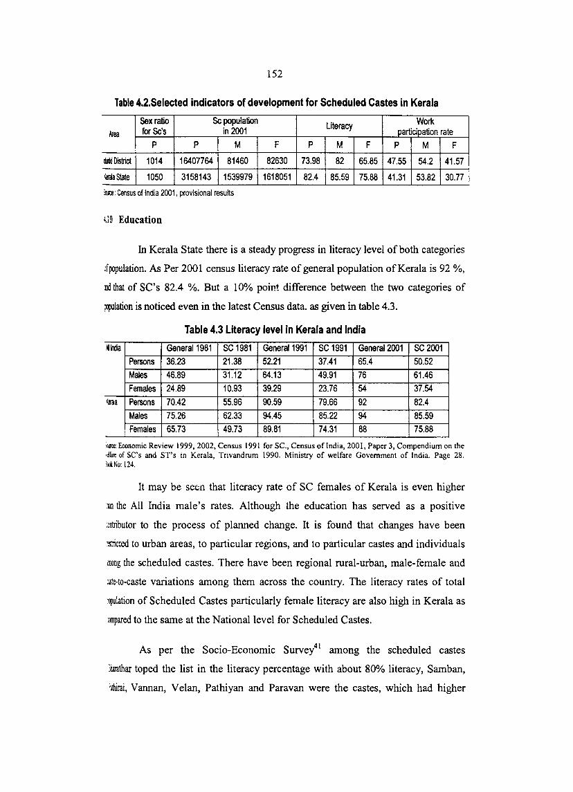
152
Table 4.2.Selected indicators of development for Scheduled Castes in Kerala
Sex ratio Se population Work Nea for Se's in 2001 Literacy
participation rate p p M F P M F P M F
tiki District 1014 16407764 81460 82630 73.98 82 65.85 47.55 54.2 41.57
l.saIaState 1050 3158143 1539979 1618051 82.4 85.59 75.88 41.31 53.82 30.77
)me: Census of India 2001, provisional results
t19 Education
In Kerala State there is a steady progress in literacy level of both categories
Jfpopulation. As Per 2001 census literacy rate of general popUlation of Kerala is 92 %,
lIXI that of SC's 82.4 %. But a 10% point difference between the two categories of
~ulation is noticed even in the latest Census data. as given in table 4.3.
Table 4.3 Literacy level in Kerala and India
IIkldia General 1981 se 1981 General 1991 se 1991 General 2001 se 2001 Persons 36.23 21.38 52.21 37.41 65.4 SO.52 Males 46.89 31.12 64.13 49.91 76 61.46 Females 24.89 10.93 39.29 23.76 54 37.54
Ifta Persons 70.42 55.96 90.59 79.66 92 82.4 Males 75.26 62.33 94.45 85.22 94 85.59 Females 65.73 49.73 89.81 74.31 88 75.88
w: Economic Review 1999,2002, Census 1991 for SC., Census of India, 2001, Paper 3, Compendium on the .dfare of SC's and ST's in Kerala, Trivandrum 1990. Ministry of welfare Government of India. Page 28. biNo: 124.
It may be seen that literacy rate of se females of Kerala is even higher
ian the All India male's rates. Although the education has served as a positive
:Jntributor to the process of planned change. It is found that changes have been
~lricted to urban areas, to particular regions, and to particular castes and individuals
~'DOng the scheduled castes. There have been regional rural-urban, male-female and
:3Ste·to-caste variations among them across the country. The literacy rates of total
Xlpulation of Scheduled Castes particularly female literacy are also high in Kerala as
:mnpared to the same at the National level for Scheduled Castes.
As per the Socio-Economic Survey41 among the scheduled castes
lIiarathar toped the list in the literacy percentage with about 80% literacy, Samban,
'Jthirai, Vannan, Vel an, Pathiyan and Paravan were the castes, which had higher

153
XltClltage of literacy in 1981.42 Castes which had literacy percentage between 70 and
~ were; Mannan, Paravan, Perumannan, Pathiyan, Vannan, and Velan. A large
X!tClltage of the literates were found only able to read and write and with out any
~ucational qualification. Table 4.4 gives the percentage of literacy between different
£ibcastes among SC's.
i rable4.4 Percentage of literacy between different sub castes among SC's.
Uo Caste % Of Literacy SI.No. Caste % of Literacy
t Bharathar 81.57 30. Kalladi 45.16 1. Samban 81.25 31. Bakuda 45.16 3. Pulhirai Vannan 81.19 32. Pallan 42.88 4. Velan 77.49 33. Gossangi 42.86 5. Palhiyan 76.03 34. Kadaiyan 41.80 6. Paravan 75.38 35. Cheruman 40.64 1. Perumannan 74.n 36. Vetan 39.73 8. Mannan 70.37 37. AdiAndhra 39.65 10. Kakkalan 68.97 38. Nayadi 38.50 11. Adi Dravida 66.30 39. Karimpalan 37.45 12 Ayyanavar 66.21 40. Nal Kadaya 34.56 13. Arulhathiyar 65.97 41. Chakkliyan 34.09 14. Samagara 65.74 42. Koalan 33.57 15. Thandan 65.51 43. Mogar 33.57 16. Pandannan 64.91 44. Baira 33.48 17. Vettuvan 62.20 45. Ajila 30.76 18. Pulayan 61.32 46 Adi karnataka 28.65 19. Valluvan 58.65 47. Domban 28.05 20. Panan 57.53 48. Koosa 23.14 11. Mundala 56.48 49. Mavilon 18.39 22. Parayan 57.53 50. Boyan 17.42 13. Pulayavettuvan 55.33 51 Gavara 14.64 24. Malayan 52.85 52. Kavara 12.14 25. Pambada 51.28 53. Holeya 7.36 26. Kuravan 49.44 54. Maila 4.37 27. Kanakkan 47.45 28. Vallon 46.81 29. Thoti 46.53
Me; report of the Commission on the Socio Economic conditions of se's and ST's of Kerala,1982, p.9
The percentage of those who have passed "matriculation or above" gave a
more realistic picture of the educational attainment. Among the Scheduled castes the
percentage of persons who have passed S.S.L.C or above was only 2.87 in 1981.43

154
~ percentages of persons of the different castes who had passed matriculation or
M'CBre given in table 4.5.
!No
1.
2.
3.
(,
5.
6.
7.
8.
9.
10.
11.
12.
13. 14.
Table 4.5 Percentage of persons who passed matriculation
or above among se's in Kerala
Caste Percentage SI.No. Caste Samban 25.00 14. Ayyanavar Puthiraivannan 11.88 15. Padannan
Paravan 8.14 16. Parayan Bharathar 7.96 17. Panan Perumannan 7.78 18. AnJnth~thivar
Ajila 7.69 19. Thandan Pathiyan 7.64 20. Padannan Velan 7.27 21. Pulayan Vannan 6.75 22. Mulyan Samugara 6.48 23. Thoti Mannan 5.52 24. PuluyaVettan Mundala 5.44 25. Kuravan Kakkalan 5.14 26. Nayadi Ayyanavar 4.85
~: Report of commission on Sc's and Sfs 1982 P. 9
Percentage 4.85 4.18 3.64 3.54 3.47 . 3.46 3.40 3.07 2.85 1.98 1.89 1.81 1.64
Among Scheduled castes, Samban is observed to be the most advanced
:me. Among Puthiraivannan 12% have passed matriculation or above. Perumannan,
Ajila, Pathiyan and Velan where found with literacy rate close to 8%. Among
?ulayar, who constitute more than 36% of SC's, only 3% have passed "matriculation
orabove".44 Thus educational progress varied widely between the various castes.
4.11 Extent of Immovable Property and Types of Houses
The extent of land owned by the Scheduled Castes households is an
:ndicator of their economic position and social status. The distribution in Idukki
District is a little different from other state with higher percentage of household in
~me castes having no land and household in some castes with higher percentage
ilaving large extent of land. Even in the case of those who owned their own land, the
ex1ent in most cases was 10 cents or so. The % of households having more than 10
cents of land is negligible in the case of most castes. It was found that the average
area of holdings of SC's in Kerala was only 0.12 hector. While that of total
!lOpulation is 0.41 hector.45 This is shown in table 4.7.

155
Table 4.6 Ownership of land and type of houses of Scheduled Castes
Uo Caste % with % huts SI. No Caste % with % huts no land no land
1. Pallan 93.78 11.16 32. Vettuvan 9.08 -1- Adikamalaka 75.54 14.90 33. Kavara 8.66 67.15 l. Chakklian 49.07 54.79 34. Kanakkan 3.28 77.75 4. Arunthathiyar 40.00 60.00 35. Thoti 8.00 29.17 5. Bakuda 35.99 46.66 36. Perumannan 7.78 32.69 6, Samban 33.33 66.67 37. Nalkdaya 7.55 85.72 7, Ayyanavar 29.09 87.71 38. Pandannan 7.26 35.90 I, Boyan 28.27 64.44 39. Malayan 6.38 76.06 9 Vannan 28.13 - 40. Samagara 6.25 SO.OO 10, Parayan 26.13 64.58 41. Vallon 6.06 69.84
1" Maila 24.34 97.81 42. Gavara 5.73 56.81 12. Pathiyan 23.55 77.94 43. Moger 5.72 80.54 13, Velan 22.93 - 44. Cheruman 5.30 80.71 14, Mannan 21.95 66.06 45. Valluvan 4.55 86.61 15. Holeya 19.48 - 46. Kootan 4.00 89.00 16. Bharathar 19.15 61.22 47. Adi Dravida 2.55 18.91 17. AdiAnddhra 19.13 91.25 48. Karimpalan 1.27 93.09 11, Kuravan 17.63 86.08 49. Ajila 0.00 100.00 19, Kakkalan 17.23 67.32 50. Gosangi 0.00 100.00 ~, Mundala 16.67 61.91 51. Dompan 0.00 94.12 21, Baira 16.22 90.54 52. Kadaiyan 0.00 67.19 12, Paravan 15.93 69.71 53. Koosa 0.00 51.62 23, Velan 14.24 57.73 54. Pampada 0.00 37.50 14, Pulayan 12.67 77.85 55. Holeya - 96.65 25, Nayadi 12.50 61.66 56 Vettuvan - 71.40 16, Puthiraivannan 11.76 29.41 57 Vannan - 62.15 17, Panan 11.74 72.58 58. Vetan - 83.52 ta, Mavilan 11.65 94.58 19, Thandan 11.57 76.13 ll, Pulaya-Vettuvan 10.25 73.70 31. Kalladi 9.37 92.63
iw: Report of the Commission, 1982
One of the basic needs of man is a house to live in with his family. The
xilities in the house are also equally important. The types of houses occupied by the
:oople of the State varies from cave like structures constructed with sheets of stone
~the tribes of Idukki district to palatial mansions in various parts of the State. The
~Ipe of houses of Scheduled castes as per the socio-economic survey46 is also
:'reSented in table 4.7.

156
The position of the two major castes Pulayan and Cheruman were not
~ bad· among them 9 and 6 percent respectively lived in pucca houses
~ximately 20% of the Scheduled Castes households lived in single room houses
~l'i households in most castes live in houses with one or two rooms. The very single
::oo! was used as Kitchen and for living and sleeping by all members of the
rousehold. The type of the house and the facilities available varied between castes.
~eofthese are quarters provided by plantation owners for their workers.
m Investment
The economic status of a community can be judged by the total income of
it households and the amount of money they are able to save. It was revealed that in
~~ofmost of the castes no household or less than five percent have bank deposits.
The Scheduled Castes populations are in the lowest economic state. Their
:lKOme is not even sufficient to meet their consumption expenditure. Hence the
~on of saving or investing does not arise in most cases.
U3 Household size
The number of persons in a household gives a broad indication of the fertility
;erel of the population since the nuclear household consists of parents and children only.
:\Iso the living conditions of the family are very adversely affected if there are a large
lIlIIber of members in a family. As per 1991 census size of the households 4.90% for
~heduled Castes of Kerala and for General population it was 5.30%.
tI4 Food habits
The health and nutritional standards of people depend on the quality and
\uantity of food consumed by them, especially on the quality of items. The items
Jsed by all the households as found by the Socio-Economic Survey were Cereals,
~pices and Salt. Since many persons belonging to Scheduled Castes are agricultural
(orkers or coolies they have to be away from their home for most of the day. They
jepend on the food available in the hotels during noon. Nutrition's item like egg,

157
milk, ghee, and other milk products and other luxurious items are not found popular,
tiththesehouseholds as per Survey 1982.47
Only less than 10 percent households in most of the castes consume eggs
IS revealed by the Survey48 Among castes that use egg in large percentage of
:x,useholds are Vannapt, Chakkiliyan, Paravan, Pallan, Pathiyan and Kanakkan. Milk
~ used by a larger percentage is households in most of the castes. Milk products are
itCII to be consumed by only a small percentage of households. In short it can be said
!hat most of the Scheduled Castes households are living on cereals, tubers and other
cheap food. The rich and nutritious food items are not common with them.
The quality of the food taken by a person affects the person'l; health
Slandard. The quality of the food depends on the resources. One can afford for food.
A group of people having very low income, cannot be expected to afford a substantial
lIDount for food. The small amount at their disposal will be utilized to purchase cheap
food. The Scheduled Castes households in the State are seen to be in the low-income
groups and are seen to be living on cheap and not nutritious food. The percentage of
households consuming milk, milk products and egg are still lower in Idukki District.
~ short, the Scheduled Castes households very rarely take food items other than
cereals and tubers as per survey.
Good health and nutritional standards of a people are essential pre
requisites for their well-being. No progress can be expected for a population if it does
not maintain a reasonable level of health standards. Scheduled Castes being put up in
poor and unhygienic circumstances and living on less nutritious food cannot be
expected to have a high-level health standard.
4.15 Use of modern garments, cosmetics and foot wear
Scheduled Castes, though inhabitants of the plains are different from the
ollter sections of the people. In ancient times, mode of dress also was peculiar to
!hem. But with the change of time much progress has been achieved. As seen from
the results of the socio-economic survey, modern garments are being used by most of
lheScheduled Castes people with a few exceptions.

158
U6 Special Programmes For Scheduled Castes in Kerala
In Kerala the initial Five-Year Plans did not had a separate component for
lte development of Scheduled Castes except for certain welfare programmes
mdertaken by the Harijan Welfare Department. Detailed guidelines for the
'reparation of a Special Component Plan for Scheduled Castes were issued as part of
:ifth Five-Year Plan.
A review of the programme reveals that the funds earmarked were
~gnificantly lower than the popUlation share and the schemes were often not relevant to
'ie local needs. It was in this background that in Kerala it was decided to decentralize
lie Special Component Plan to the district from 1983-84 onwards. District Level
Working Groups for Scheduled Castes were formally constituted. A project-based
~ach had been adopted for implementation of schemes from 2002-03 onwards.
This new approach is expected to ensure human resources development of Scheduled
* including their education and training, provision of minimum needs like housing,
Jrinking water, electricity, health care and economic development.
The Scheduled Caste Development Department is implementing various
;chemes for development of scheduled castes in Kerala. There are at present two
~pes of schemes, State schemes and State sponsored schemes. The state schemes are
~11plemented by the Department direct and the State sponsored schemes are
.mplemented through local governments. Major schemes implemented by the
)epartment can be grouped into three namely: schemes for educational development,
:mployment oriented programmers and other social development and welfare
lfOgrammes
Kerala Institute For Research, Training and Development studies is
~1Other agency mandated to conduct "A study on decentralized planning and
levelopmental activities among Scheduled Tribes ofwayanad district" and a study on
·Unemployment problem among the educated Scheduled Castes and Scheduled tribes
J Kerala". The Kerala State Development Corporation for Scheduled Castes and
~heduled Tribes is implementing about 60 types of schemes under various sectors of

159
Gevelopments for asset creation and employment generation for Scheduled Castes and
lcheduled Tribes.
U7 Summary
From time immemorial Scheduled castes have been a deprived section of our
mety. Their low status has been the bye - product of the caste system that prevail~ in
India over the years This large chunk of population has been named in different forms
Uke sudras, untouchables, exuntouchable, exterior castes, out castes depressed classes,
,,';' dal't hed led t o~,. .. ';+1.. ~t.,. -""""~,. ,.CO .:._-- 'T'I..,. """+,. ".~~., ..... "o~"'''d • iIIlIJ3I1S, 1 , se u cas es "'''''' ....... 1. .......... "" .P~~wb .... V.L ".1..1.4.£_ • .6..a.,u •• WO"".n. .... ~Jl3"\JJ.1J. .l"",u,u. ea.
~omic mobility by its insistence on hierarchy passing on of crafts and skills
During the course of the last century the institution of custe in India
undeIWent considerable changes. Independent India offered to the Scheduled castes
!he promise to a life of dignity through a number of protective measures written into
ler constitution. The majority of the Scheduled castes have not yet freed themselves
:mm the stranglehold of poverty, inequality and injustice. The division of the people
0110 four well-defined castes never existed in Kerala as is seen in the northern parts of
ildia, The principle of treating each group following a particular occupation as a
;eparate caste and of prohibiting inter marriage and interdining between them was
jtroduced in Kerala by the Aryan immigrants
People belonging to particular occupation groups were made separate castes.
lle castes, which follow low occupations, are in the lower state of social order. The
livent of British rule, the industrial revolution in the west, modem technological growth
m fast communication together with some social movements led to some changes in the
:asic social structure of the society. A major proportion of disadvantaged groups among
~iIeduled Castes still live below the basic minimum requirements.49
The general economic progress of the state has not made any appreciable
:npact on the economic condition of the majority of scheduled castes popUlation.
1ey are in the lowest level even now as in the past. The Socio-econorilic conditions
:iScheduled Castes of the State are very poor. There are much differences in the
~itions of the various sub- castes among them.

160
OTES AND REFERENCES
Agarwal Yash, (199~), "Literacy Among Scheduled Castes -Trends and Issues",
National Institute for Edocational Planning and Administration, New Delhi, India
Note: As per Census Report 1981 'General Population' refers to population other
than Scheduled Castes and Scheduled Tribes.
Sinha Surjit, (1968), "Caste in India-Its Essential Pattern of Socio-Cultural
Integration, In Caste and Race: Comparitive Approach", edited by'Antony Reuck
and Julie Knight, I and Church Hill, A, Ltd, London.
Andre Betelle, (1971), University of California Press, Berkeley.
Srinivas, M.N, (1997), "Caste in Modem India and Other Essays", Asia
Publishing Rouse, Bombay.
I. Nanda Urmi, (1992), "The Psycho-Social Parameters of Socio-Economic
Mobility and Poverty", UnpUblished Doctoral Dissertation, University of
Allahabad.
1. Dwnont, L, (1970), "Homo Hierarchy The Caste and its Implications", London.
i. Paswan Sanjay,et.al,(1999), "Encyclopedia if Dalits in India",Social Justice,
Vo1.7, PP.II-45.
Oommen, T.K,(1984), " Social Transfonnation in Rural India- Mobilisation and
State Intervation", Vikas Publishing House, New Delhi, P.118.
lOo Beegom Javernesa, M.J, (1985), "Aiyankali and the Social Awakening Among
thePulayar", Journal of Kerala Studies, Vol.Xn, Parts I-IV, PP.11-21.
:\. Celestin BougIe, (1971), "Essays on the Caste System", Translated by
Pocook,D.F, University of Sussex, P.148.
i1. Celestin BougIe, (1971), "Essays on the Caste System", Cambridge University
Press.
], More Galander, (1984), "Competing Equalities: Lwa and the Backward Classes
in India", Oxford University Press, Delhi, P.18.
1 Bharat Patnakar and Gail Omvedt, (1979), "The Dalit Liberation Movement in
Colonial Period", Economic and Political Weekly, Vol. XIV, No.8, PP.411-413.

161
Srikant, L.M, (1951) "Report of the Commissioner for Scheduled Castes and
Scheduled Tribes for the period ending 3.1 st December", Government of India.
Gandhi,M.K(1966), "Collected Works", XX,April-August 1921,Government of
India, Navjivan
Premchand, (1962), "Vividh Prasang", Vol.II, Allahabad,P.471.
Navajivan, (1924), CWMG, Vol.XXIV, June 29, P.321, Young India (1925),
CWMG, Vol.XXVI, February 5, P.73.
Navajivan, (1924), CWMG, Vol.XXIV, ~.~~)·l~,r. ~C.
Gandhi, M.K, (1945), Yeravada Mandir, Ahmedabad, Chapter IX.
Paswan Sanjay,et.al,(1999), "Encyclopedia if Dalits in India",Struggle for Self
Liberation, Vo1.2.
Paswan Sanjay,et.al,(1999Paswan Sanjay,et.al,(1999), "Encyclopedia if Dalits in
India",Social Justice, Vo1.4.
Ibid.
Bharadwaj, A.N, (1979), "Problems of Scheduled Castes and Scheduled Tribes
in India", P.11.
Government of Kerala, (1982), "Report of Commission on the Socio-Economic
Conditions of Scheduled Castes and Scheduled Tribes", YoU, Part.I,
Trivandrum, P .6.
Ibid. P.23.
Ibid. P.22.
Opcit. Bharadwaj, A.N, P.3.
Wankhede, G.G, (2001), "Educational Inequalities Among Scheduled Castes in
Maharashtra", Economic and Political Weekly, May, PP.1553-1558.
Opcit. Government of Kerala, (1982), P.30.
Census of India, (2001), Government of India, Provisional.
UNDP, Analysis of National Development Problems, India,
www.undp.org.inlreportlHDR97/hdrforcs.htm-20k.

162
: fg,vemment of Kerala, (2002), "Economic Review", State Planning Board,
Trivandrum •
. ~ ~lGovemment ofKerala, (1982), P.35.
:: Ibid. P.40.
r. fg,vemment of India,Report of the Commissioner for Scheduled Castes and
Scheduled Tribes Part-I,1975-76 and 1976-77,24th Report .
.. Opcit. Government ofKerala, (1982), PP. 9-10.
! Opclt. Census of India, (2001).
, ~ Calsus of India, (1991), "Primary Census Abstract, Scheduled Castes and
Scheduled Tribes", Series-12, Part ll-B(ii), Kerala, P.26.
( Opcil Agarwal Yash. P. 12
( Opcit. Government ofKerala, (1982), P.26.
;: Ibid. P.9.
;; Ibid. P.22.
;: Ibid. P.9 .
• ~ Ibid. P.19.
l:. Ibid. P.18.
;' Ibid. P.13.
;l Ibid. P.15 .
. ~ Opcit. UNDP, P. 28

CHAPTER. V
CONSUMPTION PATTERN OF SCHEDULED
CASTES IN INDIA AND KERALA
The existence of large disparities in living standards between regions and
between classes of people is widely believed to be an important cause of prevailing
social tensions and unrest in India. 1 Wide economic disparities have been observed
between the rich and the poor especially due to low rate of economic change among
the poorer sections of the population of India who generally fail to make use of the
development programmes.
Development policies of the government are increasingly judged not
merely by their success in achieving a rapid expansion of :lggregate real output but in
ICmlS of how the fruits of development are distributed between different classes and
regions. The inequalities that persist between poor people and rich, women and men,
rmaI and urban and among different ethnic groups are seldom isolated instead they are
mterrelated and overlapping,2 Continued efforts haven been made through five year
jevelopmental plans for the socio-economic upliftment of the people. It is in this
:ontext that a proper understanding of the level and components of per capita
;onsumption expenditure, (an indicator of the level of living) in the rural an urban area
~ attempted that could reveal whether economic disparity has increased or decreased.
Studies abound on the pattern of food and non-food consumption over the
:egions of the country Here in this chapter an attempt is made to analyse the changes
:J the consumption expenditure pattern of Scheduled Castes overtime and to see in
.hat way it differs from consumption expenditure pattern of General population3 The
Jurpose of this part is to bring out the changes in consumption, both in the level and
I :ommodities of consumption of SC's that happened in India and Kerala during the
~nt years. Also it highlights how the consumption pattern of SC's in Kerala differs
:urn that of General popUlation in Kerala and also that of SC's in all India. Here
:onsumption expenditure break-up by the same broad groups of items of consumption
ire considered as done in case of analysis of consumption pattern of the General
:opulation in Kerala in Chapter Ill.

164
Here for the analysis of consumption Pattern of Scheduled Castes
comprehensive time series data on items of consumption expenditure and distribution
of se households! population by monthly per capita total consumption expenditure is
DOl available from the NSSO or any other sources. For the first time in NSS history,
the pattern of consumption of the Scheduled Castes, their size as well as composition,
separately and in complete exclusion of the households belonging to other social
groups was provided by NSSO based on the data from its 38th round enquiry [January
-December 1983].4 The results give a firm basis for assessing the levels of l~ving of
the Scheduled Castes households which constitute the most vulnerable section in the
society. The NSSO also in its 43Ta [July 1987 - June 1988] and 50th [July 1993- June
1994] round enquiries provide data on pattern of consumption of different social
groups separately from that of other households.5 This chapter analyses the
consumption pattern of Scheduled Castes in Kerala based on the NSSO data from
three rounds covering the period January 1983 - June 1994. The concepts and
definitions followed here are as same as those used in the NSS.
The purpose of this part is to bring out the changes in consumption, both
in the level and commodities of consumption of Scheduled Castes that happened in
India and Kerala during the recent years. Also it highlights how the consumption
pattern of Scheduled Castes in Kerala differs from that of General popUlation in
Kerala and also that of Scheduled Castes in all India.
5.1 Distribution of persons by MPCE
The distribution of Scheduled Castes population by monthly per capita
consumption expenditure classes in the rural and urban areas of India and Kerala is
given in Table 5.1
Table 5.1 Percentage Population of SC below selected MPCE levels
Rural Urban State Social group % Population below % Population below
Rs. 165 Rs.210 Rs.355 Rs.230 Rs.310 Rs.605
Kera/a se 8 25 80 23 39 96
All 6 16 57 14 33 80
India se 27 50 88 32 56 91
All 19 39 80 19 39 80 SIw: Nsso.SO" round
I

165
At all India level it may be observed that 27% of the rural Scheduled
Castes population of the country as a whole were below the MPCE level of Rs.165,
S()oA, Scheduled Castes population were below the MPCE level of Rs.21 0 and 88 %
below the MPCE level ofRs. 355.
Considering all households at ~ll India level it may be observed that only
19% of the rural population of the country as a whole were below the MPCE level of
below Rs. 165, 39% of the rural population' were below the MPCE !evel of Rs. 210
and 80% below the MPCE level ofRs. 355. Hence it is found that the MPCE position
of Scheduled Castes population in the rural areas of country is consistently poorer
than that of the General population as evidenced by higher proportion of persons
falling in the lower MPCE levels.
Among the urban SC popUlation of the country as a whole 32% were in
the lowest MPCE level of below Rs. 230. 56% of the urban Scheduled Caste
population of the country as a whole were having an MPCE level below Rs. 310 and
91% of Scheduled Caste of the country belong to the MPCE level of below Rs. 605.
It may be observed that only 19% of all urban population of country were
below the MPCE level of Rs. 230 and 39% of the urban population were having an
MPCE level below Rs. 310 and 80% were with an average MPCE level below Rs. 605.
Hence it is found that the MPCE level of the Scheduled Caste population
in the urban areas of the country also is consistently poorer than that of the General
population as evide:1ced by the higher proportion of popUlation falling in the lower
MPCE levels.
The distribution of Scheduled Caste population by monthly per capita
expenditure classes in the rural areas of Kerala show that 8% of the rural Scheduled
Caste popUlation were below the MPCE level of Rs. 165. And 25% of rural
Scheduled Caste population had an MPCE level below Rs.210 and 80% of them had
anMPCE level below Rs. 355 in Kerala.
The MPCE position of the General popUlation of rural Kerala show that
only 6% were below the MPCE level of Rs.165. And 16% rural popUlation had an

166
MPCE level below Rs. 210 and 57% of them had an MPCE level below Rs. 355.
HCIICC in rural Kerala also the MPCE position of is consistently poorer than that of
:be General popUlation.
The distribution of Scheduled Caste by monthly per capita expenditure
i1asses in the urban areas of Kerala shows that 23% of the urban Scheduled Caste were
rclow the MPCE level of Rs. 230. And 39% of urban Scheduled Caste had an MPCE
:evel below Rs. 310 and 96% of them had an MPCE level below Rs. 605 in Kerala.
The MPCE position of the General population of urban Kerala show that
only 14% were below the MPCE level of Rs. 230. 33% of urban population had an
MPCE level below Rs. 310 and 80% of them had an MPCE level below Rs. 605.
Considering the different MPCE classes it is observed that in case of urban Kerala
also the MPCE position of Scheduled Caste is consistently poorer than that of
General popUlation.
S.2 Average Household size of Scheduled Castes.
Average household size of Scheduled Castes is presented in Table 5.2. As
per the Table 5.2 the average household size for Scheduled Castes in the rural sector
in India was 4.85 and for General popUlation it was 5.20 for the urban sector at the
National level the same was 4.75 for Scheduled Castes and for others it was little
higher 4.81. It is found that the average household size of Scheduled Castes was
lower than that of General population.6 Similarly for Kerala rural sector the average
household size it was 5.24 for Scheduled Castes and 5.24 for General popUlation.
Table 5.2 Average household sizes of SC's
State Average Household·size
Rural se ALL Urban se ALL
Kerala 5.24 5.32 4.89 5.12
All-India 4.85 5.20 4.75 4.81
Sourte: NSSO 38th round
For the urban Kerala the average size of Scheduled Castes households
was 4.89 which was lower than 5.12 for General population. Thus for Kerala also it is
found that Scheduled Castes have lower household size than General popUlation.

167
SJ Average monthly per capita consumption expenditure
The average MPCE for Scheduled Castes vis-a-viz the total population is
shown in Table 5.3.
a e . verage T bl 53A or c e ue as es MPCE f S h did C t Scheduled Castes General population
States Year Rural Urban Rural Urban
1983 94.31 128.95 112.31 165.80
All India 87-88 133.35 185.03 157.66 245.72
93-94 238.91 346.84 281.43 458.04
1983 105.07 133.99 145.24 178.31
Kerala 87-88 164.39 182.39 208.83 261.70
93-94 298.72 395.21 390.41 493.83
SOIIte: NSS various rounds
As per NSSO data for the 38th round [January -December 1983], the
average MPCE of Scheduled Castes in All-India was Rs.94.31 for the rural sector.
The average MPCE increased to Rs. 133.35 in 43rd round [1987-88] and as per the
50lh round it further increased to Rs. 238.91.
For the same periods for the General population the increase was from Rs.
112.31 to Rs. 157.66 and further to Rs. 281.43. It is found that the MPCE position of
Scheduled Castes is much below that of General popUlation in the rural sector in India.
Considering the rural sector of Kerala the average MPCE of Scheduled
Castes as per the NSS 38th round was Rs. 105.07. This increased to Rs. 164.39 in
1987-88 and further to Rs 298.72 in 1993-94. For the same period for the General
population the increase was from Rs. 145.24 in 1983 to Rs. 208.83 in 1987-88 and
further to Rs. 390.41 in 1993-94 in rural Kerala.
The average MPCE of Scheduled Castes are found lower than that of
General population in India as well as Kerala. As seen earlier it is also found that the
MPCE of Scheduled Castes households in All India is lower than Scheduled Castes in
Kerala. Scheduled Castes in Kerala have a comparatively better MPCE position than
their counterparts at the National level.
I
i
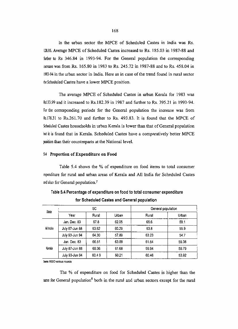
168
In the urban sector the MPCE of Scheduled Castes in India was Rs.
128.95. Average MPCE of Scheduled Castes increased to Rs. 185.03 in 1987-88 and
further to Rs 346.84 in 1993-94. For the General population the corresponding
increase was from Rs. 165.80 in 1983 to Rs. 245.72 in 1987-88 and to Rs. 458.04 in
1993·94 in the urban sector in India. Here as in case of the trend found in rural sector
the Scheduled Castes have a lower MPCE position.
The average MPCE of Scheduled Castes in urban Kerala for 1983 was
Rs133.99 and it increased to Rs.182.39 in 1987 and further to Rs. 395.21 in 1993-94.
For the corresponding periods for the General population the increase was from
Rs.l78.31 to RS.261.70 and further to Rs. 493.83. It is found that the MPCE of
Scheduled Castes households in urban Kerala is lower than that of General population
but it is found that in Kerala. Scheduled Castes have a comparatively better MPCE
position than their counterparts at the National level.
5.4 Proportion of Expenditure on Food
Table 5.4 shows the % of expenditure on food items to total consumer
expenditure for rural and urban areas of Kerala and All India for Scheduled Castes
and also for General population.7
Table 5.4 Percentage of expenditure on food to total consumer expenditure
for Scheduled Castes and General population
se General population State
Year Rural Urban Rural Urban
Jan. Dec. 83 67.8 62.05 65.6 59.1
All India July 87 ·Jun 88 63.62 60.29 63.8 55.9
July 93·Jun 94 64.30 57.89 63.23 54.7
Jan. Dec. 83 66.51 63.09 61.64 59.38
Kerala July 87 ·Jun 88 60.36 61.68 59.94 59.79
July 93·Jun 94 60.4 9 60.21 60.46 53.92
SoIree: NSSO various rounds
The % of expenditure on food for Scheduled Castes is higher than the
same for General population8 both in the rural and urban sectors except for the rural

169
india for the 43rd and 50th round. The proportion of food expenditure is found
declining for both Scheduled Castes and General population.
The % expenditure on food for Scheduled Castes in rural all India has
registered a decline from 67.8% in 1983 to 64.30 in 1993-94. For the General
lXlPulation the corresponding decline was from 65.6% in 1983 to 62.23% in 1993-94.
The decline is found more or less same for both types of households.
For urban sector for Scheduled Castes of all India the % declined for the
S3II\e period from 62.05% to 57.89%. For General households in urban sector, the
decline was from 59.1 % to 54.7% in the same period.
In Kerala as observed at the National level the % of expenditure on food
for Scheduled Castes is higher than the same of General population in both rural and
urban sectors. The proportion of expenditure on food is declining for both Scheduled
Castes and General population.
In Kerala for the rural sector for Scheduled Castes the % expenditure on
1000 showed a decline from 66.51 in 1983 to 60.49 in 1993-94 and for the General
populations for the same period the corresponding decline was from 61.64 to 60.46. It
!S found that in rural Kerala % of food expenditure declined faster for Scheduled
Castes than General popUlation.
In the urban sector for the Scheduled Castes the % expenditure on food
declined from 63.09 to 60.21 for the same period and for the General popUlation the
decline was from 59.38 to 5~.92. It is observed that % expenditure on food declined
ilSter for General population in urban Kerala than Scheduled Caste population.
S5 Proportion of Expenditure on Non - Food
The % of expenditure on non- food for Scheduled Castes is lower than the
S3II\e for General popUlation both in the rural and urban sectors. The proportion of
000· food expenditure is found increasing for both Scheduled Castes and General
population.

170
The % expenditure on non-food for Scheduled Castes in rural all India has
registered an increase from 32.2%in 1983 to 35.7% in 1993-94. For the General
population the corresponding increase was from 34.44 % in 1983 to 36.77%in 1993-
94. The increase is found more for General population.
For urban sector for Scheduled Castes of all India the % increased for the
same period from 37.35 % to 42.11%. A much more steeper increase in % was
observed. For general house holds in urban sector, the increase was from 40.9% to
45.3% in the same period.
In Kerala as observed at the National level the % of expenditure on non -
food for Scheduled Castes is lower than the same of General population in both rural
and urban sectors. The proportion of expendlture on non- food is increasing for both
Scheduled Castes and General population. Table 5.5 Shows Proportion of
Expenditure on Non - Food Items to Total Consumer Expenditure for Rural and
Urban Areas In Kerala & India
State
All India
Kerala
Table 5.5 Proportion of Expenditure on Non - Food Items to Total
Consumer Expenditure for Rural and Urban Areas In Kerala & India
se General population
Year Rural Urban Rural
Jan. Dec. 83 32.2 37.35 34.44
July 87 -Jun 88 36.38 39.71 36.2
July 93-Jun 94 35.7 42.11 36.77
Jan. Dec. 83 33.49 36.91 38.36
July 87 -Jun 88 39.64 38.32 40.06
July 93-Jun 94 39.51 39.79 39.54
Source: NSSO different rounds
Urban
40.9
44.1
45.3
40.62
40.21
46.08
In Kerala for the rural sector for Scheduled Castes the % expenditure on
non- food showed an increase from 33.49% in 1983 to 38.36 %in 1993-94 and for the
General populations for the same period the corresponding increase was from 38.36%
to 40.06%. It is found that in rural Kerala % of non- food expenditure increased much
faster for Scheduled Castes than for General popUlation over the period.
In the urban sector for the Scheduled Castes the % expenditure on non
food increased from 36.91 to 39.79 for the same period and for the General

171
population the increase was from 40.62 to 46.08. It is observed that % expenditure on
non food has increased much faster for General population in urban Kerala than
Scheduled Castes households.
Summing up, the variation in percentage expenditure on food and non
food is higher in urban areas than in rural areas.
5.6 Pattern of Consumer Expenditure of Scheduled Castes
It has already been observed that the average MPCE for Scheduled Castes
is less than that for the General population. In both rural and urban areas of Kerala,
the % of expenditure on food for Scheduled Castes households (66.51, 63.09) is
found higher than the average for General population (61.61, 58.96). Consumer
expenditure pattern of Scheduled Castes and General popUlation is presented in Table
5.6 and Table 5.7 for Kerala and all India.9
5.6.1 Rural Kerala
The Kerala rural MPCE on Cereals for Scheduled Castes Rs. 30.34 is
lower than that for General population Rs. 34.36 of Kerala. Expenditure on certain
food groups Cereals substitutes, Beverages & refreshments is higher for Kerala
Scheduled Castes than General population. The average MPCE on Milk ofRs. 5.97 of
Kerala General population is much higher than that of Kerala Scheduled Castes Rs.
2.08. Similarly the average MPCE of General popUlation of rural Kerala on Sugar,
Pulses are higher than the same of Kerala rural Scheduled Castes.
Larger differences are observed for the non-food items. The expenditure
on Pan, tobacco & intoxicants ofRs. 5.78 is higher for Kerala rural Scheduled Castes
than the same of Rs. 4.50 for Kerala rural General popUlation. The expenditure on
Fuel & light is higher for Kerala rural General popUlation, Rs. 8.45 than for Kerala
rural Scheduled Castes Rs. 7.20.
The observed differences are of much higher order for Clothing. The
average MPCE on Clothing of Rs. 9.27 of Kerala rural General population is higher
than the same for Kerala rural Scheduled Castes of Rs. 5.29. The average MPCE of
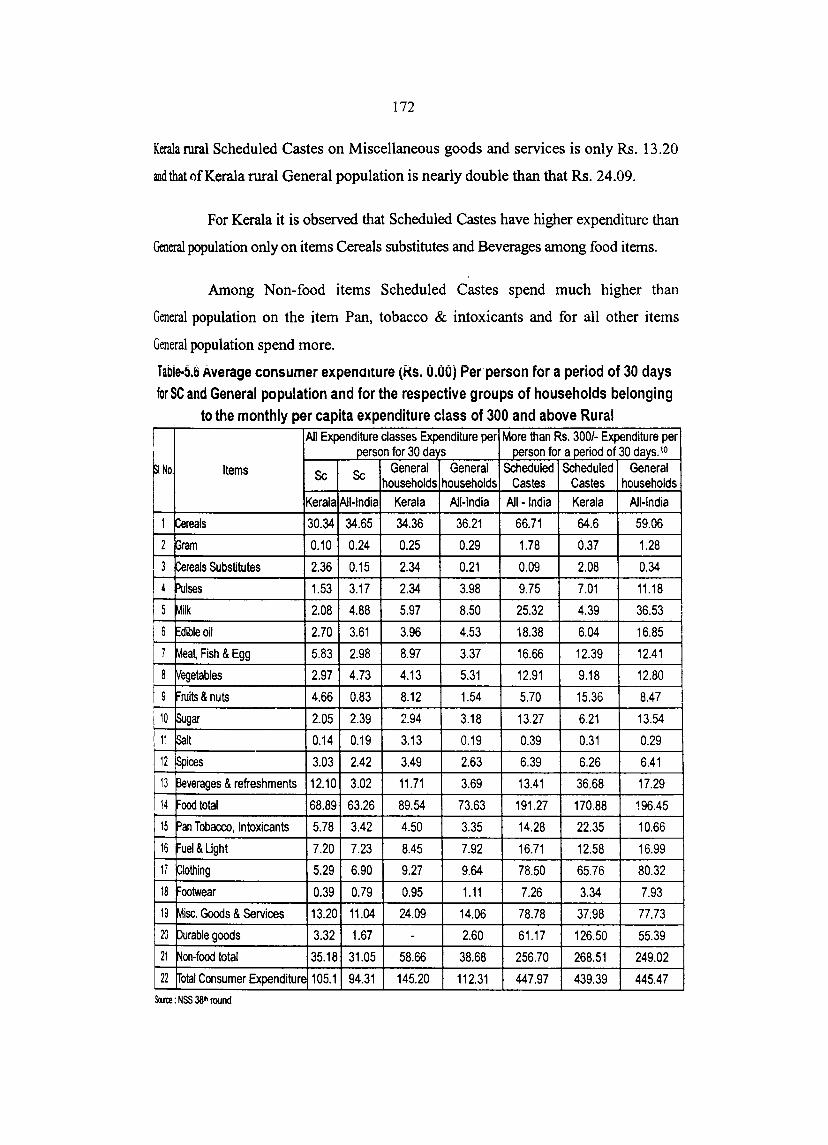
172
Kera1a rural Scheduled Castes on Miscellaneous goods and services is only Rs. 13.20
and that ofKerala rural General population is nearly double than that Rs. 24.09.
For Kerala it is observed that Scheduled Castes have higher expenditure than
General popUlation only on items Cereals substitutes and Beverages among food items.
Among Non-food items Scheduled Castes spend much higher than
General population on the item Pan, tobacco & intoxicants and for all other items
General population spend more.
Tabia-S.t; Average consumer expenalture (Rs. 0.00) Per person for a period of 30 days for se and General population and for the respective groups of households belonging
to the monthly per capita expenditure class of 300 and above Rural
I All Expenditure classe& Expenditure per More than Rs. 300/- Expenditure per person for 30 da s person for a period of 30 days.l0
S.No. Items Se Se General General Scheduled Scheduled General households households Castes Castes households
Kerala All-India Kerala All-India All-India Kerala All-India
1 Cereals 30.34 34.65 34.36 36.21 66.71 64.6 59.06
2 Gram 0.10 0.24 0.25 0.29 1.78 0.37 1.28
3 Cereals Substitutes 2.36 0.15 2.34 0.21 0.09 2.08 0.34
4 Pulses 1.53 3.17 2.34 3.98 9.75 7.01 11.18
5 Milk 2.08 4.88 5.97 8.50 25.32 4.39 36.53
6 Fdible oil 2.70 3.61 3.96 4.53 18.38 6.04 16.85
7 ~eat, Fish & Egg 5.83 2.98 8.97 3.37 16.66 12.39 12.41
8 ~egetables 2.97 4.73 4.13 5.31 12.91 9.18 12.80
9 ruits & nuts 4.66 0.83 8.12 1.54 5.70 15.36 8.47
110 ~ugar 2.05 2.39 2.94 3.18 13.27 6.21 13.54
11 ~alt 0.14 0.19 3.13 0.19 0.39 0.31 0.29
12 Spices 3.03 2.42 3.49 2.63 6.39 6.26 6.41
13 Beverages & refreshments 12.10 3.02 11.71 3.69 13.41 36.68 17.29
14 ood total 68.89 63.26 89.54 73.63 191.27 170.88 196.45
15 Pan Tobacco, Intoxicants 5.78 3.42 4.50 3.35 14.28 22.35 10.66
16 uel & Ught 7.20 7.23 8.45 7.92 16.71 12.58 16.99
17 Clothing 5.29 6.90 9.27 9.64 78.50 65.76 80.32
18 ootwear 0.39 0.79 0.95 1.11 7.26 3.34 7.93
19 ~isc. Goods & Services 13.20 11.04 24.09 14.06 78.78 37:98 77.73
20 purable goods 3.32 1.67 - 2.60 61.17 126.50 55.39
21 Non-food total 35.18 31.05 58.66 38.68 256.70 268.51 249.02
22 rrotal Consumer Expenditure 105.1 94.31 145.20 112.31 447.97 439.39 445.47
~: NSS 38"round
!
I

173
ill Pattern of consumer Expenditure for the Scheduled Castes in the Top
MPCE class:
The pattern of consumption of Scheduled Castes in this expenditure class
)IPCE >Rs. 300] is entirely different from that of the total Scheduled Castes in rural
Kerala.The average MPCE of ,total Scheduled Castes in Kerala is RsI05 whereas
~heduled Castes in the top MPCE class have an average MPCE of Rs. 440.
Expenditure on food amounted'to Rs.68.9 for the first clas3 and for the top class it is
Rs, 170.88. Expenditure on non-food amounted to Rs. 35.18 for total rural Scheduled
Castes and the same for the top class Scheduled Castes it was Rs. 268.51. The
conswnption pattern of Scheduled Castes in the top expenditure class is comparable
10 that of the general house holds in the top expenditure class in rural Kerala.1n this
lOp class Scheduled Castes s spend more on the different non -food items as similar
to the trend observed in case of General population in Kerala.
It is seen from Table 5.6 that in the top expenditure class [MPCE above
RsJOO] the average MPCE for all India rural Scheduled Castes, Rs. 448 is higher
than that of the total rural Scheduled Castes in Kerala, Rs. 440. 11 The pattern of
consumption of Kerala rural Scheduled Castes in this expenditure bracket exhibit
sharp dissimilarity to that of all India rural scheduled castes in the same expenditure
bracket. In the food group for the items Vegetables, Sugar, Pulses, Milk, Edible oil,
Meat, Fish & Egg, the MPCE of Kerala rural Scheduled Castes is much lower than
that of all India rural SC population.
In the top expenditure class the average MPCE is lower, Rs. 439, and also
MPCE on food is lower, Rs. 171, for Kerala rural schedule castes. The average
MPCE is higher, Rs. 448 and MPCE on food is also higher, Rs. 191, for all India rural
Scheduled Castes.
Relatively much higher expenditure for Kera1a rural Scheduled Caste
popUlation is reported on the food items, such as Fruits & nuts, and Beverages &
refreshments. The average MPCE of Kerala rural Scheduled Castes population on
Fruits & nuts Rs. 15.36 is more than three times the same of all India rural Scheduled
Castes population Rs. 5.70. Similarly the observed difference in the expenditure on

174
Beverages & refreshments between Kerala rural Scheduled Castes population and all
India rural Scheduled Castes population is much higher. The expenditure on Beverages
& refreshments of Rs. 36.68 for Kerala rural Scheduled Caste population are more than
double than that of all India rural Scheduled Caste population Rs. 13.41.
The average MPCE for all India rural Scheduled Caste population on
Cereals, Pulses, Milk, Edible oil, Meat, Fish & Egg, Vegetables, Sugar and Spices is
much higher than that for all Kerala rural Scheduled Castes population. The MPCE
on Milk Rs. 25.32 of all India rural Scheduled Caste population is more than five
times that of all Kerala rural Scheduled Castes population Rs. 4.39. The expenditure
on Edible oil Rs. 18.38 of all India rural Scheduled Castes population is more than
double than the some of all-Kerala rural Scheduled Castes population in the same
item. Among the non-food item group all Kerala rural Scheduled Castes population
spend larger amount on Pan, tobacco& intoxicants, Rs. 22.35.
The MPCE on Fuel & Light is higher for all India rural Scheduled Caste
population Rs. 16.71. Expenditure on Clothing is higher for all India rural Scheduled
Caste population Rs. 78.50 than the same for all Kerala rural Scheduled Castes Rs.
65.16.
The expenditure on Durable goods of Rs. 126.50 of All Kerala rural
Scheduled Caste population is more than double than that of the all India rural
Scheduled Caste population Rs. 61.17 on Durable goods. Thus it is found that rural
Scheduled Castes in the top expenditure spend more on Fruits & Nuts, Beverages
Refreshments and Processed food than their counterparts in the National level among
food items. And among non-food items they spend much higher on Pan, Tobacco &
Intoxicants and Durable goods than Scheduled Castes in the National level
5.6.3 Pattern of consumer Expenditure for the Scheduled Castes for urban
Kerala in the Top expenditure class
The pattern of consumer expenditure pertaining to the Scheduled Castes
of urban Kerala and Scheduled Castes of urban in all India are shown in Table 5.7

175
Broadly the consumer expenditure pattern of Scheduled Castes in the
iIIban areas are similar to those obtaining in the rural areas. The Kerala urban MPCE
iG Cereals for Scheduled Castes Rs. 32.86 is lower than that for General population
Rs.35.l8 of Kerala. Expenditure on certain food groups Cereals substitutes and Salt is
~gher for Kerala Scheduled Castes than General population.
The average MPCE on Milk of Rs9.02. of Kerala urban General
~pulation is much higher than that ofKerala Scheduled Castes Rs.3.67. Similarly the
!I'erage MPCE of General population of urban Kerala on Sugar, Pulses Edible oil,
\Ieat, Fish & Egg, Fruits & nuts, are higher than the sarnt;; uf KClaia w uau :;~i.l\;;uui\;;u
Castes.
Table 5.7 Average consumer expenditure (Rs. 0.00) Per· Person for a period of 30 days for Scheduled Castes and General population and fur the respective groups of house holds belonging to monthly per capita expenditure class of Rs. 300/· and above urban
All expenditure classes expenditure per > Rs. 300 expenditure per person person12
S.No. Items Se Se General General Scheduled General General population population Castes I population I population
Kerala All-India Kerala India All-India Kerala All-India
1 Cereals 32.86 31.02 35.18 31.85 46.64 43.13 38.59 2 Gram 0.17 0.28 3.37 0.31 1.03 - 0.68 3 Cereals Substitutes 0.90 0.07 0.78 0.13 0.12 1.54 0.25 4 Pulses & Products 2.11 4.62 3.02 5.32 9.95 7.42 9.11
5 Milk Products 3.67 8.52 9.02 15.27 23.66 2.52 42.12 6 dible oil 3.69 6.25 5.04 7.98 13.18 6.70 15.92 7 ~eat, Fish & Egg 7.88 5.36 11.62 5.93 17.25 15.62 14.88 8 Wegetables 3.65 6.80 4.99 8.17 14.40 10.83 16.50 9 ruits & nuts 6.23 1.72 9.76 3.48 6.67 16.35 12.75 10 ISugar 2.68 3.42 3.39 4.06 7.92 8.71 7.56 11 ~t 0.15 0.18 0.14 0.19 0.26 0.16 0.28 12 ~ices 3.27 3.07 3.76 3.36 7.43 4.55 5.66 13 ~verages &Refreshmen~ 17.27 8.70 18.44 11.26 39.47 29.61 40.18 14 cod Total 84.53 80.01 104.73 97.31 187.98 165.14 204.48 15 Pan, Tobacco Intoxicants 5.22 4.93 4.23 4.05 14.64 3.31 9.22 16 ~ght& Fuel 8.89 9.47 10.23 11.40 18.41 17.28 21.57 17 ~Iothing 6.59 9.70 14.35 12.80 73.87 60.20 65.75 18 ootwear 0.54 1.26 1.69 1.84 6.97 - 7.58 19 ~is. Goods& Services 26.31 20.56 38.13 33.85 78.30 132.20 121.36 20 purable goods 1.91 3.02 - 4.55 55.12 - 36.10 21 ~on.food 49.46 48.94 71.63 68.49 247.31 212.99 261.58 22 olal consumer
133.99 128.95 176.36 165.80 435.29 378.13 406.06 ExPenditure iM'e: NSS 38" round

176
Larger differences are observed for the non-food items. The expenditure
:nPan, tobacco & intoxic.ants ofRs.5.22 is higher for Kerala urban Scheduled Castes
~ the same of Rs. 4.23 for Kerala urban General population.
The expenditure on Fuel & Light for Kerala urban General population,
~,IO,23 than for Kerala urban Scheduled Castes Rs.8.89.
The observed differences are of much higher order for Clothing. The
lI'crage MPCE on Clothing ofRs. 14.35 of Kerala urban General population is higher
:haD the same for Kerala urban Scheduled Castes ot .Ks. 6.59. The average MPCE of
Kerala urban Scheduled Castes on Miscellaneous goods and services is Rs. 26.31 and
Iha1 ofKera1a urban general population is 38.13
For urban Kerala it is observed that Scheduled Castes have higher
apenditure than General population only on items Cereals substitutes among food
naIlS, Among non-food items Scheduled Castes spend much higher than General
population on the item Pan, tobacco & intoxicants and for all other items General
popUlation spend more.
5.6.4 Pattern of consumer Expenditure for the Scheduled Castes in the top
MPCE class of Rs.300 and above: Kerala Urban:
The pattern of consumption of Scheduled Castes in this expenditure class
~ entirely different from that of the total Scheduled Castes in urban Kerala.The
average MPCE of total Scheduled Castes in Kerala is RS.134 whereas Scheduled
Castes in the top MPCE class have an average MPCE of Rs378. MPCE on food
amounted to Rs. 84.53 for the urban Kerala and for the top class it is Rs. 165
Expenditure on non-food amounted to Rs, 49.46 for total-urban Scheduled Castes and
Ihesame for the top class Scheduled Castes it was Rs.213. The consumption pattern
of Scheduled Castes in the top expenditure class is comparable to that of the general
house holds in the top expenditure class in Kerala. In this top class Scheduled Castes
spend more on the different non -food items. This shows that among the Scheduled
Castes the higher expenditure class is exhibiting luxurious consumption pattern. Itl3 is
seen from Table 5.7 that in the top expenditure class the average MPCE for all India

177
UIban Scheduled Castes Rs. 435 is much higher than that of the all Kerala Urban
Scheduled Castes14 Rs. 378.
The pattern of consumption of Kerala urban Scheduled Caste popUlation
exhibit sharp dissimilarity to that of all India urban Scheduled Caste popUlation in the
same expenditure brackets.
In the food group only for four items, Cereals substitutes, Fruits & nuts,
Sugar, and Salt, the MPCE of Kerala rural Scheduled Castes is much lower than that
of all India rural Scheduled Caste popuiation.
In the top expenditure class the average MPCE is lower, Rs. 378 and also
MPCE on food is lower, Rs.165. for Kerala urban schedule castes. The average
MPCE is higher, Rs. 435 and MPCE on food is also higher, Rs.188, for all India
urban Scheduled Castes.
Relatively much higher expenditure for Kerala rural Scheduled Castes
population is reported on the food items, such as Cereals substitutes, Fruits & nuts,
and Sugar. The average MPCE of Kerala rural Scheduled Castes population on Fruits
& nuts Rs. 16.35 is more than double the same of all India rural Scheduled Castes
population Rs. 6.67. The observed difference in the expenditure on Beverages &
refreslunents between Kerala Scheduled Castes population and all India Scheduled
Castes popUlation is much higher. The average MPCE for all India urban Scheduled
Caste population on Cereals, Pulses, Milk, Edible oil, Meat, Fish & Egg, Vegetables,
Sal~ Beverages & Spices is much higher than that for all Kerala urban Scheduled
Castes popUlation.
Among the non-food item group all Kerala urban Scheduled Castes
population spend larger amount only on Miscellaneous goods and services, 15
Rs.l32.20 while that of the Scheduled Castes in India is only Rs.78.30 nearly half of
that of Scheduled Castes in Kerala. The MPCE on all other non-food items is higher
for all India urban Scheduled Castes population.
Expenditure on Clothing is higher for all India urban Scheduled Castes
population Rs. 73.87 than the same for all Kerala urban Scheduled Castes Rs.60.20.

178
Thus it is found that urban Scheduled Castes in the top expenditure class
!peIId more only on Cereals substitutes Fruits & Nuts and Sugar than their
counterparts in the National level among food items. And among non-food items they
spend much higher on Miscellaneous goods than Scheduled Castes in the National
level. This shows the particular pattern of consumption among the urban Scheduled
Castes of Kerala.
5.6.5 Pattern of Consumer Expenditure of Scheduled Castes and General population
5.6.6 India.
There is a wide range of variation between the rural MPCE of scheduled
castes and General popUlation. While there is not much variation in the case of
cereals, there is considerable variation in the case of milk & milk products and other
commodities this is shown in table 5.6. Expenditure on Cereals is higher for the
General population 36.21 than for Scheduled Castes 34.65 at all India level.
Larger differences are observed for the non-food items. The expenditure
on Pan, tobacco & intoxicants is higher for Scheduled Castes Rs. 3.42 than for
General popUlation Rs. 3.35 but the difference is not that high as that observed in
Kerala between the same two set of households.
The expenditure on Fuel & light is higher for General popUlation Rs. 7.92
than for Scheduled Castes Rs. 7.23. The observed difference is of a much higher
order for Clothing. Rs. 6.90 for Scheduled Castes and Rs. 9.64 for General
population.
The average MPCE of Rs. 14.06 on Miscellaneous goods and services for
the General popUlation is perceptibly higher than that for Scheduled Castes. The
expenditure for the General population is again higher for Footwear and Durable
goods at all India level.
Thus it is found that at the National level in the rural sector the General
population spends more than Scheduled Castes on all food items. Among non-food
Scheduled Castes spend more than General popUlation only on Pan, & intoxicants.

179
;.6.7 Pattern of consumption expenditure for the Scheduled Castes in the
MPCE class of Rs. 300 and above.All- India rural
The pattern of consumption of Scheduled Castes in this expenditure class
Hntirely different from that of the total Scheduled Castes in rural India The average
IIPCE of total Scheduled Castes in India is Rs.94 whereas Scheduled Castes in the
lIlMPCE class have an average MPCE ofRs 448. Expenditure on food amounted to
M3.26 for the first class and for the top class it is Rs, 191.27. Expenditure on non
;))(\ amounted to Rs 31 for total rural Scheduled Castes and the same for the top
:!ass Scheduled Castes it was Rs256.7. The consumption pattern of Scheduled Castes
Jthetop expenditure class is comparable to that of the general house holds in the top
:xpenditure class in rural India. In this top class Scheduled Castes s spend more on
:\editTerent non -food items.
It is seen from Table 5.6 that the average MPCE for the Scheduled Castes
00 General popUlation in the top expenditure class is very close to Rs. 4501-. The
:m5ponding amount Rs. 445 for General population is lower than the same for
~heduled Castes Rs. 448. It is interesting to note that the pattern of consumption of
~heduled Castes in this expenditure bracket unlike that for the total Scheduled
:astes, exhibit close similarity to that of General population. For most of the item
;oups the MPCE of Scheduled Castes is higher than the corresponding MPCE of the
:eneral popUlation. In the top expenditure class, the average MPCE of general
:ouseholds is lower Rs. 445 while MPCE on food is higher Rs. 196 for General
»pulation. The average MPCE is higher Rs. 448 and MPCE on food is lower Rs. 191
:lr Scheduled Castes.
Relatively higher expenditure is reported for Scheduled Castes on
:ereals, Edible oil, Meat, Fish & Egg. In spite of the fact that they belong to top
:xpenditure class the MPCE on Milk for the, the Scheduled Castes population is
:)llJjd substantially lower compared to General population
Among non-food items, Scheduled Castes spend larger amount on Pan,
~ & intoxicants Rs.14.28. The MPCE on the item for General population is only
~, 10.66 It is further observed that the MPCE on Fuel & light is of the order of Rs. 17

180
il the two groups of population being studied. Scheduled Castes MPCE for the item
):able goods is Rs.61.17 while the same for General population is Rs.55.39 only.
From the foregoing analysis it can be concluded that the consumption
~em of Scheduled Castes in the top expenditure class is entirely different from the
_ for total Scheduled Castes in rural India. They spend higher than General
Xipulation in rural sector at National level on food items such as Cereals, Edible oil,
I ~!eat, Egg & Fish, and Hon-food items such as Pan& intoxicants, and Durable goods.
7nus they exhibit similar or even better consumption standards as compared to
General popUlation in the rural sector at the National level.
~6.8 Pattern of consumer expenditure for the Scheduled Castes Urban: - All India.
The pattern of consumer expenditure pertaining to the Scheduled Castes
md to General population of the urban areas of India are shown in Table 5.7. It is
e\ident from the table that the amount spent on food items have declined while the
amount spend on most of non-food items especially Miscellaneous goods have
:ncreased considerably over the years.
Miscellaneous goods, Durable goods and non-food total are the items
:ound to be consumed at an increased rate than earlier round. Durable consumption in
urban India is higher than that of urban Kerala. In case of Clothing consumption the
expenditure incurred by Scheduled Castes of urban Kerala is more than that of
Scheduled Castes of urban India. Compared with Scheduled Castes of urban Kerala
Footwear consumption is found to be less in urban India.
Broadly the deviation in the consumer expenditure pattern of Scheduled
Castes compared to that of the General popUlation in the urban areas are similar to
those obtaining in the rural areas. In value terms the average MPCE in the urban areas
~ nearly one half times of that in rural areas for General popUlation. For Scheduled
Castes the corresponding proportion is 1.36.
The all India urban MPCE on Cereals for the two groups that is Scheduled
Castes and General popUlation are very close. Expenditure on Cereals is higher for the
General population 31.85 than for Scheduled Castes 31. 02 at all India level.

ISI
Expenditure on all the food-groups is higher for the General population.
The avenge MPCE on Milk and Milk products of Rs. 15.27 for the all India rural
_ population is more than double of that for Scheduled Castes Rs. 8.52
Expenditure on Pulse & Products, Edible oil, Fruits & nuts, Vegetables,
Sugar & Beverages are also higher for the General population The average MPCE on
3cverages of Scheduled Castes households Rs. 8.70 is much lower than the same for
General population Rs. 11.26.
Larger dltterences are observed tor the non-food items. Pan, tobacco &
:nlOxicants is the only item for which average MPCE of Scheduled Castes is higher
Rs.4.93, than for General population Rs. 4.05 but the difference is not that high as
that observed in Kerala between the same two sets of households.
The expenditure on Fuel & light is higher for General population Rs.
! 1.40 than for Scheduled Castes Rs.9.4 7. The observed difference is of a much higher
order for Clothing Rs. 9.70 for Scheduled Castes and Rs12.S0 for General population
The average MPCE ofRs. 33.85 on Miscellaneous goods and services for
die General population is perceptibly higher than for Scheduled Castes 20.56 The
expenditure for the General population is again higher for Footwear and Durable
goods at all India level.
Thus it is found that in the urban sector in India Scheduled Castes are
much behind General population in expenditure on almost all items except Pan &
intoxicants.
5.6.9 Pattern of consumer expenditure in the MPCE class of Rs. 300 and above
for urban India
The average MPCE in the top MPCE class for the General popUlation and
the popUlation belonging to Scheduled Castes are Rs. 406.06 arid Rs. 435.29
respectively. Agreement and dissimilarities among the MPCE on different groups of
items for the two popUlation groups in the urban areas exhibit close similarity with
the same top expenditure class of the rural areas.

182
The pattern of consumption of Scheduled Castes in the top expenditure
class is entirely different from that of the total Scheduled Castes in urban India. The
average MPCE of total Scheduled Castes in India is Rs.129 whereas Scheduled
Castes in the top MPCE class have an average MPCE ofRs. 435.29. Expenditure on
food amounted to Rs. 80.01 for the first class and for the top class it is Rs. 187.98.
Expenditure on non-food amounted to Rs. 48.94 for tutal urban Scheduled Castes and
the same for the top class Scheduled Castes it was Rs. 247.31.
The consumption pattern of Scheduled Castes in the top expenditure class
~ comparable to that of the General population in the top expenditure class in urban
India. In this top class Scheduled Castes spend more on the different non -food items
as similar to the trend observed in case of General population. This shows that among
the Scheduled Castes the higher expenditure class is exhibiting luxurious
consumption pattern.
It is seen from Table 5.7 that the average MPCE for the Scheduled Castes
in the top expenditure class is Rs.435.29. The corresponding amount Rs. 406.06 for
General population is lower than the same for Scheduled Castes. It is interesting to
note that the pattern of consumption of Scheduled Castes in this expenditure bracket
unlike that for the total Scheduled Castes, exhibit close similarity to that of General
population. For most of the item groups the MPCE of Scheduled Castes is higher than
the corresponding MPCE of the General popUlation. In the top expenditure class, the
average MPCE is lower Rs. 406 and MPCE on food is higher Rs. 204.48 for General
population. The average MPCE is higher Rs. 435 and MPCE on food is lower Rs. 189
for Scheduled Castes.
Relatively higher expenditure is reported for Scheduled Castes on
Cereals, Gram, Pulses, Meat, Fish & Egg, Sugar and spices, in spite of the fact that
they belong to top expenditure class the MPCE on Milk for the, the Scheduled Castes
population is found substantially lower compared to General popUlation ..
Total non-food expenditure of the Scheduled Castes Rs. 247.31 is found
higher than that of General population, Rs. 261.58 Among non-food items, Scheduled

183
Castes in the top expenditure class spend larger amount on Pan, tobacco& intoxicants.
Clothing, and also Durable goods.
From the foregoing analysis it can be concluded that the consumption
pattern of Scheduled Castes in the top expenditure class in All-India is entirely
different from the same for total Scheduled Castes in the urban sector also. In the top
expenditure class they exhibit better consumption standards as compared to General
population in the urban sector at the National level.
Considering the consumption standards of the total Scheduled Castes
population it is found that they are still below general households in both India and
Kera1a. On the other hand considering the consumption standards in the top
expenditure class, Scheduled Castes are found possessing similar and even better
standards than General population in the same expenditure categories. Comparison of
consumption standards of Scheduled Castes population in India and Kerala shows
that Scheduled Castes in Kerala are possessing relatively better consumption
standards than their counterparts in India but have yet a long way to go to reach the
standards of the other general households.
5.7 Per capita expenditure
5.7.1 Kerala
Table 5.8 gives Per capita expenditure in on broad groups of food anQ
non-food items and % to total expenditure in Kerala for Scheduled Castes & General
population Looking at the 38th round data given here a picture of average rural and
urban consumption pattern for Scheduled Castes and General population for Kerala
emerges.
Thus it is found that t he per capita expenditure of Scheduled Castes of
rural Kerala Rs. 105.07 is found to be much lower than that of General popUlation Rs.
145.20. While average monthly expenditure on food of Scheduled Castes amounted
only to Rs. 69.89 per month, that of General population was Rs. 89.54. Food
expenditure constituted 66.51 % of total consumption expenditure for Scheduled
Castes and only 61.67% for General popUlation. Of the food expenditure, expenditure

184
)!1 Cereals constituted 28.87% for Scheduled Castes and only 24.01% for General
~ulation. Among food items average monthly expenditure of Scheduled Castes was
~gher than the others only for the items Beverages & refreshments and Spices.
Regarding non-food items expenditure of Scheduled Castes was higher
:haD that of General population, only on Pan, tobacco & intoxicants. Exr~nditure on
\!iscellaneous items by Scheduled Castes Rs. 12.56 amounted only to half of the
:xpenditure on the same item by General population Rs. 24.09. While the per capita
expenditure on Clothing by General population of rural Kerala constituted 6.38% of
:olal expenditure for the Scheduled Castes the same was only 5.03%. Hence among
non·food items Scheduled Castes spend more only on Pan, tobacco & intoxicants.
9No
1
2
3
4
5
6
7
8
9
10
11
12
13
14
15
16
17
18
19
20
; 21
: 22
Table 5.8 Per capita expenditure in (Rs) on broad groups of food and non·food items and % to total expenditure in Kerala for Schedulet' Castes & General population
Rural Urban
Item General population Scheduled Castes General population ~eduled Castes
Rs % Rs % Rs % Rs %
Cereals 34.36 24.01 30.34 28.87 35.18 19.95 32.86 24.52
Gram 0.25 0.17 0.1 0.09 3.37 1.91 0.17 0.12
Cereals Subst. 2.34 1.61 2.36 2.24 0.78 0.44 0.9 0.67
Pulses 2.34 1.61 1.53 1.45 3.02 1.71 2.11 I 1.57
Milk & Products 5.97 4.11 2.08 1.97 9.02 5.11 3.67 2.73
dible oil 3.96 2.73 2.7 2.56 5.04 2.86 3.69 2.75
Meat, Egg & Fish 8.97 6.18 5.83 5.54 11.62 6.59 7.88 5.88
~egetable 4.13 2.84 2.97 2.82 4.99 2.83 3.65 2.72
ruils & nuts 8.12 5.59 4.66 4.43 9.76 5.53 6.23 4.64
~gar 2.94 2.02 2.05 1.95 3.39 1.92 2.68 2
~alt 3.13 2.16 0.14 0.13 0.14 0.08 0.15 0.11
~pices 3.49 2.40 3.03 2.88 3.76 2.13 ·3.27 2.44
~verages & refreshments 11.71 8.06 12.1 11.51 18.44 10.46 17.27 12.88
ood Tota! 89.54 61.67 6989 66.51 104.73 59.38 84.53 63.08
Pan, Tobacco, & Intoxicants 4.50 3.10 5.78 5.50 4.23 2.4 5.22 3.89
uel & light 8.45 5.82 7.2 6.85 10.23 5.8 8.89 6.63
Clothing 9.27 6.38 5.29 5.03 14.35 8.14 6.59 4.91
ootwear 0.95 0.65 0.39 0.37 1.69 0.96 0.54 0.4
Misc.goods& Services 24.09 16.59 13.2 12.56 38.13 21.62 26.31 19.63
Durable goods 11.30 5.79 3.32 3.15 3 1.70 1.91 1.42
Non-food total 58.66 38.33 35.18 33.48 71.63 40.62 49.46 36.91
otal expenditure 145.20 100 105.07 100 176.36 100 133.99 100 Source: 38" NSSO.
i I

185
It is found that per capita expenditure of Scheduled Castes of urban
Kerala (Rs.l33.99) is found to be much lower than that of General population
(h.l76.36). While average monthly expenditure on food of Scheduled Castes
amounted only to Rs. 84.53 per month that of General population was Rs. 104.73.
Food expenditure constituted 63.08% of total consumption expenditure for Scheduled
Castes and only 59.38% for General pupulation. The expenditure on Cereals
:onstituted 24.52% for Scheduled Castes and only 19.95% for General popUlation
among food items average monthly expenditure of Scheduled Castes was higher than
General popUlation on the items Cereals substitutes & Salt. vu i:111 uilu:a ii.taul) UCln:adl
~pulation expenditure is higher than that of Scheduled Castes.
Regarding non-food items expenditure of Scheduled Castes was higher
!ban that of General population only on Pan, tobacco & intoxicants. While
~diture on Miscellaneous items by Scheduled Castes constituted to 19.63% of
iJIal expenditure, the expenditure on the same item by General popUlation was
:1.62%. While the per capita expenditure on Clothing by General popUlation of urban
Kerala constituted by 8.14% of their total expenditure for the Scheduled Castes only
!.91%. Thus among non-food items Scheduled Castes spend more on Pan, tobacco &
:ntoxicants than General population in urban Kerala.
lA Percentage expenditure on food items to total food
Table 5.9 shows % expenditure on different items of food to total food.
~nditure for Scheduled Castes and General population in rural and urban Kerala.
For Scheduled Castes of rural Kerala the Table 5.9 reveals that the %
:1pCnditure on Cereals has been 43.40%, which is higher than that of General
:qJulation 38.93%. Among different items of food, Scheduled Castes of rural Kerala
~rted higher % expenditure on items Cereals, Cereals Substitutes and Beverages &
~hments. For Cereals substitutes the % expenditure of rural Scheduled Castes
'is 3.36% and that of General popUlation was 2.61 % of total food expenditure. For
·~uled Castes of rural Kerala Beverages & refreshments constituted 17.30% of
lir food expenditure, while that of General popUlation was only 12.08%. For
);heduled Castes % expenditure on Pulses was 2.18%, while that of General

186
.on2.61%. For Scheduled Castes Meat, Egg & Fish constituted 8.32% of their
00d expenditure. While that of General population only 10.02%. On all other items
)f food Scheduled Castes of rural Kerala reported lower % expenditure than the
Gcneral population of rural Kerala.
Table 5.9 reveals that for urban sector Scheduled Castes % expenditure on
lmals has been 38.87% which is much higher than that of General population
],59%. For Scheduled Castes the % on Cereals substitute also was 1.06% higher
:nanthatofO.74% General population in urban Kerala.
For Scheduled Castes Beverages & refreshments constituted 20.41% of
I :heir food expenditure. While that of General population 17.61 %. Only other items of
Scheduled Castes of urban Kerala reported lower % expenditure than the General
;x!pulation f urban Kerala.
For the Scheduled Castes in both rural and urban sectors a change in the
panem of consumption is observed over the years The proportion of food in their
consumption basket is going on declining. Proportion of expenditure on non- food
Items is found increasing. The increase in expenditure is visible especially in case of
Scheduled Castes belonging to higher income groups. They are found to be following
~econsumption pattern of General population.
Table 5.9 Percentage Expenditure on different items of food to total food expenditure for Schj!duled Castes and General population in Kerala
I Rural Urban :; No. Item General Scheduled General Scheduled
population Castes population Castes 1 ~reals 38.93 43.40 33.59 38.87 2 ~ram 0.28 0.135 3.22 0.19 3 ~reals Substitute 2.61 3.36 0.74 1.06 4 Pulses 2.61 2.18 2.88 2.48 5 ~ilk & Products 6.67 2.96 8.61 4.32 6 dible oil 4.42 3.84 4.81 4.35 7 ~eat, Egg & Fish 10.02 8.32 11.18 9.32 8 ~egetable 4.61 4.23 4.76 4.31 9 ruits& Nuts 9.07 6.66 9.32 7.35 10 ISugar 3.28 2.93 3.24 3.17 11 ~It 3.5 0.19 0.13 0.17 12 ~pices 3.9 4.33 3.59 3.86 13 ~verages & refreshments 12.08 17.30 17.61 20.41 14 ood total 100 100 100 100 SMe NSS; 38'" round

187
~9 Movement in Budge share Kerala
Expenditure on some broad groups items and % to total expenditure of
Scheduled Castes in the rural and urban areas ofkerala for the period 1983 -1987-88
~~venin Table 5.10 changes that have taken place in the consumption pattern of
Scheduled Castes over the years have been analysed here with the available to study
!he differences in the changes that have occurred in the consumption pattern in the
rural and urbimJ<.erala. 16 Table 5.10 gives the movement in budget share of
Scheduled Castes in Kerala. The following points are observed.
a) It is found that the expenditures have increased over the years on all the items
both in the rural and urban areas as may be expected due to the price rise in
general.
b) In tenns of % there has been a decline in the proportion of expenditure on food
from 66.5 % in 1983 to 60.36 % in 1987-88 in the rural Kerala
c) In respect of non-food items the % expenditure has increased from 33.48 % in
1983 to 39.68 % in 1987-88
d) In the food group the items attracting more expenditure were Beverages &
refreshments, Meat, fish & egg, Vegetables, Fruits & nuts, Edible oil, Spices and
Sugar.
e) In the non-food group the % of expenditure on Clothing has declined from 5.03
%in 1983 to 4.64% in 1987-88.
In the case of urban areas also similar patlern has been observed.
a) The proportion of expenditure on food has declined from 63.08% in 1983 to
61.68% in 1987-88.
b) Among the non-food items the % of expenditure increased from 36.91% in 1983
to 38.31 % in 1987 - 88.
Looking at the available data given here for Scheduled Castes in Kerala, a
picture of average rural and urban consumption patterns for the state as a whole
emerges. The following are main features.

188
Table 5.10 Per capita per month (30 days) expenditure in (Rs. 0.00) of food and non-food items and % to total expenditure for Scheduled Caste households in Kerala.
I9-No Item Rural Urban
1983 1987-88 1983 1987-88
1 ~reals PCE 30.34 3S.04 32.86 33.0S
% 28.87 21.31 24.S2 18.12
2 ~ram PCE 0.10 - 0.17 -
I % 0.09 - 0.12 -3 ~reals substitutes
PCE 2.36 - 0.9 -% 2.24 - 0.67 -
4 Pul!ocs PCE 1.S3 - 2.11 -
% 1.45 - 1.57 -5 ~ilk & Products
PCE 2.08 - 3.67 -, % 1.97 - 2.73 -
6 ~dible oil PCE 2.70 - 3.69 -% 2.56 - 2.75 -
:
~eat. Egg, Fish PCE 5.83 - 7.88 -7
, % 5.54 - 5.88 -I
8 Wegetables PCE 2.97 - 3.65 -
i % 2.82 - 2.72 -9 ruits & nuts
PCE 4.66 - 6.23 -i I % 4.43 - 4.64 -
10 ~ugar PCE 2.05 - 2.68 -
i % 1.95 - 2 -i 11 ~alt
PCE 0.14 - 0.15 -% 0.13 - 0.11 -
12 ~pices PCE 3.03 - 3.27 -i % 2.88 - 2.44 -,
PCE 12.10 17.27 13 ~verages & refreshments - -% 11.51 - 12.88 -
14 ood Total PCE 69.89 99.24 84.53 112.51 % 66.51 60.36 63.08 61.68
15 Pan& Intoxicants PCE 5.78 - 5.22 -% 5.5 - 3.89 -
I 16 ight& Fuel PCE 7.20 - 8.89 -% 6.85 - 6.63 -
I 17 ~Iothing PCE 5.29 7.64 6.59 10.94 % 5.03 4.64 4.91 5.99
16 ootwear PCE 0.39 0.83 0.54 1.56 % 0.37 0.50 0.4 0.85
, PCE 13.20 26.31 19 ~is. Goods& Services - -% 12.56 - 19.63 -
I 20 purable goods PCE 3.32 8.25 1.91 2.13 % 3.15 5.01 1.42 1.16
I 21 ~on-food PCE 35.18 65.15 49.46 69.88 % 33.48 39.68 36.91 38.31
:22 ~otal consumer Expenditure PCE 105.07 164.39 133.99 182.39 % 100 100 100 100
Soon:e : NSS diflereni rounds
9M data not available

189
For rural Kerala per capita 30 days consumer expenditure was split up
into 66.51%for food and 33.48% for non-food. Food included 28.87% for Cereals and
11.51 % for Beverages and 5.54 % for Meat, fish & egg. Non-food included 3.32%
for Miscellaneous goods and services and 5.5% for Pan & intoxicants.
For the urban sector average MPCE was split up into 63.08%for food and
36.91 for non-food. Of food, 24.52%went towards Cereals and 12.88% for Beverages
& refreshments, and 5.88% on Meat, fish & e~g. Non- food included 19.63% for
Miscellaneous goods and services and 3.89% for Pan, tobacco & intoxicants.
Table 5.11: Per capita consumption (%) of different items in Kerala for Scheduled Castes
I % expenditure for 30 days U-R
I SI. No Item Rural Urban Difference
1983 1983
1 ~reals 28.87 24.52 -4.35
2 ~ram 0.09 0.12 0.03
3 ~reals substitutes 2.24 0.67 -1.57
4 Pulses 1.45 1.57 0.12
5 ~ilk & Products 1.17 2.73 0.76
6 ~dibleoil 2.56 2.75 0.19
7 ~eat, Egg, Fish 5.54 5.88 0.34
8 ~egetables 2.82 2.72 0.1
9 Fruits & nuts 4.43 4.64 0.21
10 lSugar 1.95 2 0.05
11 ~It 0.13 0.11 -0.02
12 ISpices 2.88 2.44 -0.44
13 ~verages & refreshments 12.51 12.88 1.37
14 ood Total .66.51 63.08 -3.43
15 Pan& Intoxicents 5.5 3.89 -1.61
16 ight& Fuel 6.85 6.63 -0.22
17 !clothing 5.03 4.91 -0.12
18 ootwear 0.37 0.4 0.03
19 ~is. Goods& Services 12.56 19.63 7.07
20 purable goods 3.15 1.42 -1.73
21 ~on-food 33.48 36.91 3.43
22 ~otal consumer Expenditure 100 100 0
SouR:e: NSSO 38th round
Of the gap between urban and rural MPCE of Scheduled Castes in Kerala,
which is of the order ofRs. 28.92 as much as Rs.14.64 was accounted by Food total.
Non-food total accounted for only Rs. 14.28 of the difference. Non-food expenditure

190
t _ in the urban sector exceeded that of the rural sector only by the extent of
li J;S. Miscellaneous good accounted for Rs. 13.11 % of the difference. Per c~pita
'_lUre on Durable goods and Pan, tobacco & intoxicants in the urban sector
lI!:ixmd less than that in rural sector.
(:; Movement in Budget Share - All-India.
Expenditure on some broad groups items and % to total expenditure of
~uled Castes in the rural and urban areas of India 17 for the period 1983 -1993-94
!P~ in Table 5.12
; It is found that expenditures have increased over the years on all items the both
m the rural and urban areas as may be expected due to the price rise in general.
~. In terms of % there has been a fall in the proportion of expenditure on food of
Scheduled Castes from 67% in 1983 to 65% in 1987-88 and 64.88% in 1993-94
ID Ihe rural areas at all - India level.
In respect of non-food items the % expenditure has increased from 32.92% in
1983 to 34.78 % in 1987-88 and 35.19 in 1993-94
.;' In the food group the item attracting more expenditure are Milk & milk products,
Vegetables, Edible oil, Pulses, Beverages, Meat, fish & egg.
In the non-food group the % of expenditure on Durable goods has increased from
1.77 % in 1983 to 2.55 % in 1987 - 88 and declined to Rs.2.1 in 1993-94.
In the non-food group the % of expenditure on Clothing has declined from 7.31
%in 1983 to 5.69 % in 1987 - 88 and declined to Rs. 4.6 in 1993-94
In case of urban areas also similar pattern has been observed. The proportion of
expenditure on food has declined from 62.04 % in 1983 to 60.29 % in 1987-88
and further declined to Rs.57.89 in 1993-94. The proportion of expenditure on
non-food has increased from 37.95% in 1983 to 39.70% in 1987-88 and to Rs.
42.24 in 1993-94.

191
Table 5.12 Per capita per months (30 days) expenditure in (Rs. 0.00) of food and non-food items and % to total expenditure for Sch~uled Castes All India
Ht! Item
1 !cereals
2 ~
J !Cereals & substitutes.
4 Pulses
I lMilk & Products
6 dibleoil
7 Meat, fish & egg
8 l"egetables
9 ruits & nuts
10 Sugar
11 lsalt
12 Spices
13 Beverages & refreshments
14 oodTotal
15 Pan Tobacco& Intoxicants
16 Fuel & light
17 Clothing
18 Footwear
19 Mi5. Goods & Services
20 Durable goods
21 Non-food
22 ~otal Consumer Expenditure
Siute. NSS vanous rounds
_ data not available
1983 PCE 34.65 % 36.70
PCE 0.24 % ".25
PCE 0.15 % 0.15
PCE 3.17 % 3.36
PCE 4.88 % 5.17
PCE 3.61 % 3.82
PCE 2.98 % 3.15
PCE 4.73 % 5.01
PCE 0.83 % 0.88
PCE 2.39 % 2.53
PCE 0.19 % 0.20
PCE 2.42 % 2.56
PCE 3.02 % 3.20
PCE 63.26 % 67.07
PCE 3.42 % 3.62
PCE 7.23 % 7.67
PCE 6.90 % 7.31
PCE 0.79 % 0.83
PCE 11.04 % 11.70
PCE 1.67 % 1.77
PCE 31.05 % 32.92
PCE 94.31 % 100
Rural Urban 1987-88 1993-94 1983 1987-88 1993-94 40.35 66.64 31.02 36.26 62.1 30.25 27.89 24.05 19.59 17.93
- 0.37 0.28 - 0.57 - 0.15 0.21 - 0.16 - 0.14 0.07 - 0.24 - 0.05 0.05 - 0.06 - 9.36 4.62 - 12.09 - 3.91 3.58 - 3.49 - P.d2 A"? ?t; t;t; - .. -...
- 7.29 6.60 - 7.37 - 10.72 6.25 - 16.29 - 4.49 4.84 - 4.7 - 7.98 5.36 - 14.27 - 3.34 4.15 - 4.12 - 15.65 6.80 - 21.41 - 6.55 5.27 - 6.18 - 2.99 1.72 - 6.54 - 1.25 1.33 - 1.88 - 7.06 3.42 - 9.16 - 2.95 2.65 - 2.64 - 0.51 0.18 - 0.59 - 0.21 0.13 - 0.17 - 6.51 3.07 - 8.02 - 2.72 2.38 - 2.31 - 9.49 8.70 - 23.69 - 3.97 6.74 - 6.84
86.97 154.83 80.01 111.56 200.53 65.21 64.88 62.04 60.29 57.89
- 9.26 4.93 - 13.24 - 3.87 3.82 - 3.82 - 18.83 9.47 - 24.73 - 7.88 7.34 - 7.14
7.59 11.01 9.70 10.56 16.26 5.69 4.6 7.52 5.70 4.69 1.18 1.73 1.26 1.89 3.28 0.88 0.72 0.97 1.02 0.947 - 38.2 20.56 - 78.23 - 16.19 15.94 - 22.58
3.41 5.04 3.02 6.06 10.57 2.55 2.1 2.34 3.27 3.05
46.38 84.05 48.94 73.47 146.31 34.78 35.19 37.95 39.7 42.24 133.35 238.91 128.95 185.03 346.34
100 100 100 100 100

192
Looking at the data available given here a picture of average rural and
urban consumption patterns of the Scheduled Castes for the country as a whole
emerges. The following are the main features.
For rural India per capita 30 days consumer expenditure was split up into
64.88%for food and 35.19% for non-food. Food included 27.89% for Cereals, 7.29%
Ior milk and products. Non-food included 16.19%for Miscellaneous goods and
5el'VlCes.
Table 5.13. Value (%) of per capita consumption of different groups of items in rural and urban India for Scheduled Castes
S.No Item % expenditure Rural % expenditure Urban U-R
1993-94 1993-94 Difference
1 ~reals 27.89 17.93 -9.9tj
2 ~ram 0.15 0.16 0.01
3 ~reals subs!. 0.05 0.06 0.01 4 Pulses 3.91 3.49 -0.42 5 ~ilk & Product 7.29 7.37 0.08 6 dibleoil 4.49 4.7 0.21 7 Meat, Egg, Fish 3.34 4.12 0.78 8 Vegetables 6.55 6.18 -0.37 9 Fruits & nuts 1.25 1.88 0.63 10 Sugar 2.95 2.64 -0.31 11 Salt 0.21 0.17 -0.04 12 Spices 2.72 2.31 -0.41 13 Beverages & refreshments 5.97 6.84 2.87 14 Food Total 64.88 57.89
, -6.99
15 Pan Tobacco& Intoxicants 3.87 3.82 -0.05 16 Light & Fuel 7.88 7.14 -0.74 17 Clothing 4.6 4.69 0.09 18 Footwear 0.72 0.947 0.227 19 Mis. Goods & Services 16.19 22.58 6.39 20 Durable goods 2.1 3.05 0.95 21 Non-food 35.19 42.24 7.05 22 Total Consumer Expenditure 100 100 0 _: NSS various rounds
I
I
For the urban sector average MPCE was split up into 57.89%for food and
i2.24 % for non-food. Of food only 17.93% went towards Cereals and 7.37% on milk
:nd products. Non-food included 22.58% for Miscellaneous goods,. Rural
!xpenditure levels per capita exceeded urban levels for Cereals, pulses, vegetables,

193
sugar and spices Among non-food for Pan, Tobacco &Intoxicants rural expenditure
~ceeded that of urban .. Non-food expenditure per person in the urban sector was
mout double that in the rural sector. Similarly per capita average expenditure on
Durable goods in urban Sector was double than that in rural sector.
ill Percentage Expenditure on food to total food expenditure and items of
Don-food to total non-food expenditure in India
The composition of total expenditure on food items over different years
snows changes ID pattern ot consumption. As per Table 5.14 in India in the rural
sector the % expenditure on Cereals has declined over the period under study.
Table 5.14 Percentage expenditure on items of food to total expenditure and on items on non-food to total non-food expenditure in India
Item Rural urban
1983 1993-94 1983 1993-94 : Cereals 54.71 43.04 38.76 30.96
Gram 0.37 0.23 0.33 0.28 , Cereals subst. 0.22 0.09 0.08 0.12 , Pulses 5.00 6.04 5.77 6.02 , Milk and Products 7.7 10.97 10.63 12.74 ; Edible oil 5.69 6.92 7.8 8.12 • Meat. Fish & Egg 4.69 5.15 6.68 7.11 I Vegetables 7.46 10.10 8.49 10.67
Fruits & nuts 1.31 1.93 2.14 3.26 Sugar 3.77 4.55 4.27 4.56
I Salt 0.29 0.33 0.2 0.29
Ispce 3.81 4.20 3.83 3.99-: Bever:ges & refreshments 4.77 6.12 10.86 11.81
Food Total 100 100 100 100 Pan & intoxicants 10.996 11.01 10.065 9.04 Fuel & Light 23.298 22.48 19.341 16.90 Clothing 22.21 13.09 19.82 11.11 Footwear 2.521 2.05 2.55 2.24 Mise. Goods services 35.54 45.44 42.00 53.46 Durable goods 5.376 5.99 6.166 7.22 Non-food total 100 100 100 100
Sourre: NSS various rounds
I
Increase in % of expenditure has been observed in respect of non-food
items. Among food items the highest % is for Cereals followed by milk and products
and vegetables for Scheduled Castes of rural India in 1993-94. Increase in %
expenditure on Miscellaneous goods and Pan & Intoxicants and Durable goods is

194
observed. The % of expenditure on Clothing declined from 22.21 % in 1983 to
13.09% in I 993-94. % expenditure is found highest among non-food items for
Miscellaneous good s for Scheduled Castes of both urban and rural India.
The table shows that in the urban sector the % of expenditure on food
declined. For Cereals the decline was from 38.76% in 1983 to 30.96 % inI993-94.
Among food items the highest % was for Cereals followed by milk and products and
Beverages for Scheduled Castes in urban India in 1993-94.
Increase in % of expencllture observed m case ot non-food items.
Expenditure on Miscellaneous goods increased from 42% in 1983 to 53.46% in 1993-
94 for Scheduled Castes in urban India. The increase in Durable goods % was not that
bigh as in case of Miscellaneous goods in both rural and urban sectors. The % of
expenditure on Clothing declined form 19.82% in 1983 tol1.11 in 1993-94.
5.13 % Expenditure on food items to total food expenditure and items of non
food to total non-food expenditure in Kerala
The following Table 5.15 present per capita per month expenditure of
broad groups of food items and % to total food expenditure and % of expenditure on
items of non-food to total non-food expenditure in rural and urban areas of Kerala.
The Table 5.15 reveals thatl8 in the rural sector the % of expenditure on
Cereals has declined from 43.40% in 1983 to 35.31% in 1987-88. Increase in % of
expenditure has been observed in respect of Durable goods from 9.41 % in 1983 to
12.63% in 1987-88. The % of expenditure on Clothing declined from 15.02% in 1983
to 11.69% in 1987-88.

195
Table 5.15 Percentage Expenditure of Scheduled Castes on items of food to total food expenditure and items of non-food to total non-food expenditure in Kerala
9. No. Item Rural Urban
1983 1987-88 1983 1987-88 1 Cereals 43.4 35.304 38.87 29.37 2 Gram 0.135 - 0.19 -3 Cereals s.ubst. 3.36 - 1.06 -,
4 Pulses 2.18 - 2.48 -5 Milk and Products 2.96 - 4.32 -6 Edible oil 3.84 - 4.36 -7 Meat, Fish & Egg 8.32 - 9.32 -8
\, ___ .. _LI __ . "., - 4.35 -vC\jtaaun::;, ".Lv
9 Fruits & nuts 6.66 - 7.35 -10 Sugar 2.93 - 3.17 -11 Salt 0.19 - 0.17 -12 Spices 4.J3 - 3.86 -13 Beverages & refreshments 17.3 - 20.41 -14 Food Total 100 100 100 100
Pan Intoxicants 16.43 - 10.54 -Fuel & Light 20.46 - 17.96 -
17 Clothing 15.02 11.69 13.30 15.64 18 Footwear 1.11 1.26 1.08 2.22 19 Misc. Goods services 37.51 - 53.18 -20 Durable goods 9.41 12.626 3.85 3.03 21 Non-food total 100 100 100 100
iIIm!: NSS different rounds
I
The % of expenditure on Footwear increased from 1.11 % in 1983 to
1.26% in 1987-88. The table reveals that in the urban sector % of expenditure on
Cereals had declined from 38.87% in 1983 to 29.37% 1987-88. In urban Kerala
Il1Crease in % of expenditure had been observed in respect of Clothing from 13.3% in
1983 to 15.64% in 1987-88. In case of Footwear also increase in % of expenditure
had been observed from 1.08% in 1983 to 2.22% in 1987-88. The % of expenditure
on Durable goods increased from 3.85% in 1983 to 3.03% in 1987-88
5.14 Expenditure on food
A comparison of the % of food expenditure in total consumer expenditure
in for Scheduled Castes is done in Table 5.16.
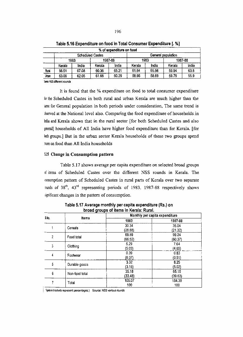
I
196
Table 5.16 Expenditure on food in Total Consumer Expenditure [. 0/0] % of expenditure on food
Scheduled Castes General population 1983 1987-88 1983 1987-88
Kerala India Kerala India Kerala India Kerala India Rural 66.51 67.08 60.36 65.21 61.64 65.56 59.94 63.8 Urban 63.09 62.05 61.68 60.29 58.96 58.69 59.79 55.9
iute: NSS different rounds
It is found that the % expenditure on food to total consumer expenditure
ior the Scheduled Castes in both rural and urban Kerala are much higher than the
same for General population in both periods under consideration, The same trend is
observed at the National level also. Comparing the food expenditure of households in
India and Kerala shows that in the rural sector [for both Scheduled Castes and also
general] households of All India have higher food expenditure than for Kerala. [for
both groups.] But in the urban sector Kerala households of these two groups spend
more on food than All India households
5.15 Change in Consumption pattern
Table 5.17 shows average per capita expenditure on selected broad groups
of items of Scheduled Castes over the different NSS rounds in Kerala. The
consumption pattern of Scheduled Castes in rural parts of Kerala over two separate
:ounds of 38th, 43rd representing periods of 1983, 1987-88 respectively shows
lignificant changes in the pattern of consumption.
Table 5.17 Average monthly per capita expenditure (Rs.) on roa_grou~s 0 I ems In era a: ura. b d f't' K I R I
~.No. Items Monthly per capita expenditure
1983 1987·88
1 Cereals 30.34 35.04 (28.88)
I (21.32)
2 Food total 69.89 99.24 (66.52) I (60.37)
3 . Clothing 5.29 7.64 (5.03) (4.65)
4 Footwear 0.39 0.83 (0.37) (0.51)
5 Durable goods 3.32 8.25 (3.16) (5.02)
6 Non-food total 35.18 65.15 (33.48) (39.631
7 Total 105.07 164.39 100 100
I =9IRSin brackets represent percentages.) Source: NSS various rounds
,
I I

197
It is evident from the Table 5.17 that the amount spent on many items had
meased considerably over the years. Cereals, Footwear, Durable goods and non-.
, food total are found to have increased than earlier rounds. This shows the changes
that have occurred in consumption pattern of Scheduled Castes of Kerala since 1983.
During the span between 1983 and 1987 - 88 a shift in the emphasis of consumption
of Scheduled Castes is obvious. Increased expenditure on non-food items namely,
Durable goods, Footwear etc. are indicative of the rising standard of consumption.
The expenditure ratio of food and non-food items had also changed
showing a decrease in the food consumption and an increase in non-food
consumption. The ratio in 1983 was 66:33. It was 60:40 in 1987-88. Table 5.18 shows
the average per capita expenditure on selected broad groups of items for Scheduled
Castes ofKerala in the urban areas.
Table 5.18 Average per capita expenditure (Rs) on
aelected broad groups of items urban Kerala.
SI. No. Items
1 Cereals
2 Food total
3 Clothing
4 Footwear
5 Durable goods
6 Non-food total
7 Total
IFvures in brackets represent percentages.) SoIree: NSS various rounds
i
Monthly per capita expenditure 1983 32.86
(24.52) 84.53
(63.09) 6.59
(4.91 ) 0.54
(0.40) 1.91
(1.43) 49.46
(36.91) 133.99
100
1987·88 33.05
(18.12) 112.51 (61.68) 10.94 (5.99) 1.56
(0.85) 2.13
(1.17) 69.88
(38.31) 182.39
100
The consumption pattern of Scheduled Castes in the urban regions Kerala
is also seem to have changed since 1983 Non-food items, Clothing Footwear, durable
good etc. are found to have gained more acceptance among the urban Kerala
consumers than food items. As different from what was observed for rural Scheduled
Castes the Clothing expenditure of urban Scheduled Castes had increased from 1983
to 1987-88. Cereals consumption of an urban Scheduled Castes in Kerala is found to
have declined ... Increase in expenditure on Durable goods was recorded here also.
The expenditure ratio of food and non-food items of Scheduled Castes in urban areas
ofKerala also had changed 63:37 in 1983 to 62:38

198
i.J~ All India
Table 5.19 Average per capita expenditure (Rs.) on selected items in Rural India 1 Monthly per capita consumption expenditure
ilt.11 Item 1983 1993-94
~5 PCE 34.65 66.64 % 36.70 27.89
, Gram PCE 0.24 0.37 % 0.25 0.15
Cereals subs!. PCE 0.15 0.14 % 0.15 0.05
I Pulses PCE 3.17 9.36 % 3.36 3.91
. ~ilk & Product PCE 4.88 17.42 , % 5.17 7.29
i Edible oil PCE 3.61 10.72 % 3.82 4.49
1 Meat, Egg, Fish PCE 2.98 7.98 % 3.15 3.34
i ~egetables PCE 4.73 15.65 % 5.01 6.55
9 Fruits & nuts PCE 0.83 2.99 % 0.88 1.25
10 Sugar PCE 2.39 7.06 % 2.53 2.95
11 Sail PCE 0.19 0.51 % 0.20 0.21
11 Spices PCE 2.42 6.51 % 2.56 2.72
13 Beverages & refreshments PCE 3.02 9.49 % 3.20 3.97
I 14 Food Total PCE 63.26 154.83 I % 67.07 el88
, 15 Pan Tobacco& Intoxicants PCE 3.42 9.26
% 3.62 3.87 I
16 Light & Fuel PCE 7.23 18.83 % 7.67 7.88 1
17 Clothing PCE 6.90 11.01 % 7.31 4.6 --
I
18 Footwear PCE 0.79 1.73 % 0.83 0.72
19 Mi5. Goods & Services PCE 11.04 38.2 % 11.70 16.19
./'il Durable goods PCE 1.67 5.04 % 1.77 2.1
11 Non-food PCE 31.05 84.05 % 32.92 35.19
112 ~otal Consumer Expenditure PCE 94.31 238.91 % 100 100
l1IIII. NSS vanous rounds

199
Table 5.20 Average per capita expenditure on selected broad groups of items in urban India . ,.
-9. No Item
Monthly per capita consumption expenditure 0"~ 1983 1993-94 "t~
1 ~als PCE 31.02 62.1 '~
% 24.05 17.93
2 ~m PCE 0.28 0.57 % 0.21
, 0.16 I
I
3 Cereals subst. PCE 0.07 0.24 I
% 0.05 0.06
4 Pulses PCE 4.62 12.09 % 3.58 3.49
5 Milk & Product PCF 8.52 25.55 % 6.60 7.37 i
6 ~dibleoil PCE 6.25 16.29 % 4.84 4.7
7 Meat Egg, Fish PCE 5.36 14.27 % 4.15 4.12
8 Vegetables PCE 6.80 21.41 % 5.27 6.18
9 Fruits & nuts PCE 1.72 6.54 % 1.33 1.88
10 Sugar PCE 3.42 9.16 % 2.65 2.64
11 Salt PCE 0.18 0.59 i
% 0.13 0.17 I I
12 PCE 3.07 8.02 , Spices
% 2.38 2.31 I
13 Beverages & refreshments PCE 8.70 23.69 I % 6.74 6.84 I
14 Food Total PCE 80.01 200.53 % 62.04 57.89 i
15 Pan Tobacco& Intoxicants PCE 4.93 13.24 ----J % 3.82 3.82 I
i
16 Light & Fuel PCE 9.47 24.73 i % 7.34 7.14 I
I
17 Clothing PCE 9.70 16.26 I
% 7.52 4.69 i 18 Footwear PCE 1.26 3.28
% 0.97 0.947 i
19 Mis. Goods & Services PCE 20.56 78.23 % 15.94 22.58
,
20 Durable goods PCE 3.02 10.57 % 2.34 3.05
21 Non-food PCE 48.94 146.31 % 37.95 42.24 i
22 Total Consumer Expenditure PCE 128.95 346.34 I % 100 100 I
SM:e: NSS different rounds
Table 5.19 shows average per capita expenditure on selected broad groups
of items for Scheduled Castes population in rural India.

200
Table 5.20 India shows average per capita expenditure on selected broad
goups of items for Scheduled Castes population in urban India.
It is evident from the Table 5.20 that the amount spent on food items have
declined while the amount spend on most of non-food items especially Miscellaneous
~ have increased considerably over the years.
Miscellaneous goods, Durable goods and non-food total are the items
I iound to be consumed at an increased rate than earlier round. Durable consumption in
illban India is higher than that of urban Kerala. In case of Clothing consumption the
expenditure incurred by Scheduled Castes of urban Kerala is more than that of
Scheduled Castes of urban India. Compared with Scheduled Castes of urban Kerala
Footwear consumption is found to be less in urban India.
5.17 Conclusions
It is found that the MPCE position of Scheduled Castes population in the
rural as well as urban areas of All-India is consistently poorer than that of the General
population as evidenced by higher proportion of persons falling in the lower MPCE
levels. Similarly in rural as well as urban Kerala als0 the MPCE position of
Scheduled Caste population is consistently poorer than that of the General population.
It is found that the average household size of Scheduled Castes was lower
than that of General population in India as well as Kerala. Comparison of MPCE of
Scheduled Castes if. India and Kerala showed that the MPCE of Scheduled Castes is
lower than that of General population in Kerala in both rural and urban sectors. But
Scheduled Castes in Kerala have a comparatively better MPCE position than their
counterparts at the National level regarding MPCE on various items.
In India as well as Kerala the % of expenditure on food for Scheduled
Castes is higher than the same for General population both in the rural and urban
sectors. The proportion of food expenditure is found declining for both Scheduled
Castes and General population

201
The % of expenditure on non- food for Scheduled Castes is lower than the
same for General population both in the rural and urban sectors. The proportion of
oon· food expenditure is found increasing for both Scheduled Castes and General
population. Among Non-food items scheduled castes spend much higher than General
population on the item Pan, tobacco & intoxicants and for all other items General
population spend more.
The consumption pattern of Scheduled Castes in the top expenditure class
~ comparable to that of the general households in rural Kerala. In this top class
Scheduled Castes spend more on the different non -food items as similar to the trend
observed in case of General population in Kerala. At the National level in the rural
sector the General households spend more than Scheduled Castes on all food items.
Among non-food, Scheduled Castes spend more than General !lopulation only on
Pan, & Intoxicants. It is found that in the urban sector also in India Scheduled Castes
are much behind General population in expenditure on almost all items except Pan&
Intoxicants
In the top expenditure class they spend higher than General popUlation in
rural sector at National level on food items such as Cereals, Edible oil, Meat, Egg &
Fish. and non-food items such as Pan& intoxicants, and Durable goods. Thus they
exhibit similar or even better consumption standards as compared to General
population in the rural sector at the National level.
The consumption pattern of Scheduled Castes in the top expenditure class
is comparable to that of the General popUlation in the top expenditure class in urban
India. In this top class Scheduled Castes spend more on the different non -food items
as similar to the trend observed in case of General popUlation. This shows that among
the Scheduled Castes the higher expenditure class is exhibiting luxurious
consumption pattern.
Considering the consumption standards of the total Scheduled Castes
population it is found that general house holds are far better in both India and Kerala
Considering the consumption standards in the top expenditure class Scheduled Castes
are found possessing similar and even better standards than General population in the

202
i3IIle expenditure bracket. Comparison of consumption standards of Scheduled Castes
~ation in India and Kerala shows that Scheduled Castes in Kerala ar~ possessing
belter consumption standards than their counterparts in India.
The per capita expenditure of Scheduled Castes of rural Kerala is found to
~ much lower than that of General population. Food expenditure constituted 66.51 %
Jftotal consumption expenditure for Scheduled Castes and only 61.67% for General
))pulation. Of the food expenditure, expenditure on Cereals constituted 28.87% for
Scheduled Castes and only 24.01 % for General population. Per capita expenditure of
Scheduled Castes of urban Kerala is found to be much lower than that of General
lIOPulation. Food expenditure constituted 63.08% of total consumption expenditure
for Scheduled Castes and only 59.38% for General population. The expenditure on
Cereals constituted 24.52% for Scheduled Castes and only 19.95% for General
lIOpulation

203
SOTES AND REFERENCES
1. Vaidyanathan, A, (1974), "Some Aspects of Inequalities in Living Standards in
Rural India". Statistical Publishing Society. PP.215-241.
1 UNDP.(1998), "Human Development Report", Oxford University Press, New
York,P.29.
i. Note: Other than Scheduled Castes
~. NSSO,(1989), "Survey Result On: A Note On Pattern of Consumer Expenditure
of Scheduled Caste and Scheduled Tribe Households", based on 38th round
(January-December) data, Sarvekshana,(January 1989-March 1989), P.l.
i. (a) NSSO,(1998), " Level and Pattern of Consumer Expenditure" based on 50th
round data, Sarvekshana, Issue No.74, VoI.XXI,No.3,January-March.
(b) NSSO, (1993), Sarvekshana, Issue No.57, VoI.XVII, No.2, October
December.
~. (a) NSSO,(1989), "Survey Result On A Note On Pattern of Consumer
Expenditure of Scheduled Caste and Scheduled Tribe Households", based on 38th
round (January-March) data,Sarvekshana,P.6,P.8.
NSSO,(1993), " 43rd round data, Sarvekshana, 5th Issue, Vol.XVII, No.2,
October-December.
;. Note: Households other than Scheduled Castes.
9. Note: Data on individual items of expenditure for Scheduled Castes not
published for different rounds in NSS, hence 38th round data alone presented
here.
:0. Note: Data for General Population of Kerala in this class not available.
il. Note: For comparing the MPCE of Scheduled Castes and General Population in
the top expenditure class in Kerala data on MPCE of General Population in top
class not available. Hence here MPCE of Scheduled Castes in Kerala is
compared with that of Scheduled Castes in India.
12. Note: Data for General Population of Kerala in this class not available.

204
13. Note: Columns 5,6.
14. Note: For comparing the MPCE of Scheduled Castes and General Population in
the top expenditure class in Kerala data on MPCE of General Population in top
class not available, hence here MPCE of Scheduled Castes in Kerala compared
with that of Scheduled Castes in India is given.
15. Note: Data on expenditure of durable goods is available.
16. Note: These two surveys were carried out during January-December 1983, July
1987-June 1988. Data on consumption expenditure of Scheduled Castes in
Kerala were available only for the 38th and 43rd rounds. In the 43rd round data
detailed items of per capita expenditure w~re published only for total Cereals,
Food-total, Clothing, Footwear, Durable goods non-food total and total
expenditure, while for the 38th round, data on expenditure on all items were
published. For the 50th round data on expenditure of Scheduled Castes have not
been published.
17. Note: For this part data from 50th round (1993-1994) on per capita per month
expenditure of different items of expenditure of Scheduled Castes for all India
have been presented.
18. Note: Data of 1993-1994 for Kerala Scheduled Castes not published.

CHAPTER VI
SOCIO ECONOMIC BACKGROUND AND CONSUMPTION
PATTERN OF SAMPLE SCHEDULED CASTE
HOUSEHOLDS IN IDUKKI DISTRICT
The development policy in India is based on the premise of "growth with
equity". It did not take much time for the development planners in India to realize the
bi-directional linkages between social well-being and economic development.. The
policy of protective discrimination was intended to reduce the vast inequalities
between the Scheduled Castes and other strata of Indian society. Its express purpose
was to enable the Scheduled Castes, to educate themselves and seek secular
employment so that they may be free of their traditional shackles l .
The outcome of social and economic reforms is uneven and far from
satisfactory as far as achievement of the Stated goals is concerned. In India a large
section of population continues to be out side the reach of development programmes
and is yet to be reached by the State driven initiatives. The share of population
lacking basic facilities is still large- most of whom are below the poverty line. The
statutory defined Scheduled castes constitute a major share of those below poverty
line despite the fact that the framework of socio-economic development adopted five
decades ago was biased in their favour.
6.1. Characteristics of Sample Households.
The primary data collected from sample households are being analysed in
this chapter to study the socio-economic background and consumption pattern of
Scheduled Caste households. A study of the socio-economic characteristics of the
households is necessary to assess the general levels of living of the sample
households. An expJanation of the characteristics of the sample Scheduled Caste
households selected is presented here.

206
bol.1 Sex wise Distribution of Sample Households
The sex - wise distribution of the sample Scheduled Caste households is
presented in table 6.1
Table 6.1 Sex wise Distribution of Sample Households
Category No. Of se hhds selected Sample Population
M F T
RURAL 100 231 239 470
URBAN 100 181 241 422
TOTAL 200 412 480 892
lwte: Survey Data
In the sample of 100 SC households selected from rural area the total
population is 470 persons. The number of males was 231and the number of females
239. In the sample 100 SC household selected from urban area the total population is
422 persons. The number of males was 181 and the number of female 241. The total
population for urban and rural sample together was 892.
Females out number males in both rural and urban sample areas. The sex
ratio observed in the sample rural and urban sectors is different from the sex ratio for
the district as a whole. As per 1991 Census of India the sex ratio in Idukki district is
993 females per 1000 males. Idukki is one of the two districts where sex ratio is in
iavour of males.
6.1.2 Sub Castes
There are 68 sub castes among the Scheduled Castes in Kerala. Their
distribution is found in all the districts in Kerala. Table 6.2 give the community wise
distribution of sample rural and urban Scheduled caste households. There are 10
communities identified the rural SC sample selected. Of them Pulaya community
~one constituted 48%.· Others constituted 52%. Among the urban Scheduled caste
sample households there are 11 communities identified and Pulaya alone constituted
62% and others 34%.

207
Table. 6.2 Distribution of sample Se households into different sub- castes (Of.)
% Of households.-Caste
Rural Urban
:1.Pcravan 21.00 10.00
~Pulaya 48.00 62.00
!3. VeIan 14.00 7.00
~.Cheramar 3.00 -15. Sambavan 1.00 1.00
i6.Parayan 8.00 1.00 I
:7. Kanakkan - c:nn
i8. Kakkalan - 5.00
9. Chaklian 1.00 4.00
10.Panan 2.00 2.00
l1.Padanna 1.00 1.00
112. Vettuvan 1.00 1.00
~ 100 100 _: SulVey data
Among the 12 communities identified in the total sample of 200
households, 9 were found in both rural and urban sectors. Pulayas constituted the
highest share of % of sample rural (48%) and urban (62%)households. The second
highest share was Paraven (21 %)in rural and (10%) in urban. The next highest share
was to Velan (14%) in rural and (7%)in urban.
6.1.3 Size of sample households
The standard of living of a household depend up on not only the level of
income but also on the size of the household. Table 6.3 gives the average household
size in the sample rural and urban areas
Table 6.3 Average household size in rural and urban areas
Average Household Size
Rural 4.70
Urban 4.22
Total 4.5
Source: SUNey data.

208
Average household size is found to be 4.7 for rural area and 4.2 for the
urban area in the survey area. The average household size is found to be higher in
rural area than urban. This is in tune with the average household size for Scheduled
Castes for the country as a whole namely, 4.9 for rural areas and 4.5 for urban areas2•
For Scheduled Castes of Kerala the average household size was 4.6 and 4.4 in rural
and urban Kerala respectively. Table 6.4 presents size distributioh of sample
households for rural and urban areas
Table 6.4. Size distribution of sample households.
Number of members Number of households
Rural Urban
1 0 0
2 8 5
3 24 11
4 31 33
5 23 25
6 9 15
7-9 4 11
10& above 0 1 ScIn: Survey data
31 % of the sample households in the rural and 33% in urban have a size
of 4 members per household. None of the sample households had an average size
below 2 members. 8% of households in rural and 5% in urban have an average size of
~ persons per household.
Only 1 % of households in urban sector had an average size of 10 and
above. In the rural sample none of the households had an average size> I 0 members.
6.1.4 Age structure of sample population
The age-structure of sample population is given in Table 6.5. In the rural
area 21.91% of the sample population belonged to age group 0-14. The age group 15-
;9 constituted 70.64% of sample population. 7.45 % of sample population in rural
were in the age group 60 and above.

209
In the urban areas 0 - 14 age group constituted 18.48% of sample
population and 71.56% of sample population were in the age group 15-59. In the
wan sector 9.95% of population were in the age group 60 & above.
Table No 6.5 Age Structure of Sample Population. (%). % of population
Average group Rural Urban
Male Female Total Male Female Total
1·14 43.69 56.31 21.91 48.72 51.28 18.48 15-59 51.51 48.49 70.64 42.38 57.62 71.56
6O&above 42.86 57.14 7.45 35.71 64.29 9.95 Total 49.15 50.85 100 42.89 57.11 100
5G11a!: Survey data.
6.1.5 Distribution of Persons in the Sample Households Based on Education.
The Scheduled Castes communities are among the least literate social
groups in the State as per Census of India 2001, 82.4% of the Scheduled caste
populations have acquired the most elementary skills in reading and writing3.
Explanations that are offered for the relatively poor spread of education
among Scheduled Caste communities largely center around factors that lie "out side" the
School system. Poverty and immiserisation of majority of the Scheduled Caste
population of the their denigrated social status, illiterate home environments and
apathetic attitudes towards education are seen to be largely responsible for the poor
response to schooling from these communities. Such arguments often tend to ignore the
distinct historical experience of Scheduled Caste communities particularly in the context
of education. These are the ex-untouchable communities that have traditionally been
denied accesses to learning, specifically because of their pqsition in the Indian caste
sttucture. Though schooling was "fonnally" open to all communities in the 1850's, the
education of the "untouchables" proceeded at a snail's pace. Report and studies have
docwnented the social opposition to the early schooling of the 'untouchables' as well as
the social and economic constrains that impede their education even today.
The status of a community depends to a certain degree on the educational
level of its members. Education not only qualifies people for better jobs, but also
creates an awareness of opportunities open to them, which enriches life4• Education is

210
considered to be the most important factor in the ladder of social mobility. It is widely
mpted that Education plays an important role in social mobility both vertical and
ixlrizontal The lowest income groups typically have not been able to have the same
effective access to primary education as the higher-income groups, because for them,
(a) the opportunity cost (Labour) of primary education is higher, (b) the benefit from
primary education is lower, (c) the private rate of return to them from such education
is lower hand at the same time (d), cost of capital against which such rate of return
must be compared, is higher than for the higher income groupss. In the case of
Scheduled Castes, education offers the possibility [V1 :'V".iC1~ <1~V<Ul"'~U1~Ui.. Tabit;; 6.6
~ves the distribution of persons in the sample households based on education.
Table 6.6. Distribution of Person in the Sample Households Based on Education %.
Rural Urban E1ucational qualification
M F T M F T
Illiterate 15 29 44 14 56 70 (3.2) (6.2) (9.4) (3.3) (13.3) (16.6)
Below V 52 46 98 41 32 73 (11.1 ) (9.8) (20.9) (9.7) (7.6) (17.3)
V-SSLC 134 127 261 104 109 213 (28.5) (27.0) (55.5) (24.6) (25.8) (50.5)
Pre Degree 12 20 32 13 31 44 (2.6) (4.3) (6.8) (3.1) (7.3) (1004)
Graduates 4 - 4 4 7 11 (0.9) (O.O) (0.9) (0.9) (1.7) (2.6)
Post Graduates 1 - 1 1 1 2 (0.2) (0.0) (0.2) (0.2) (0.2) (0.5)
TechnicaV professional - 1 1 - - 0 (0.0) (0.2) (0.2) (0.0) (0.0) (0.0)
Any other 231 239 470 181 241 422 (2.8) (3.4) (6.2) (0.9) (1.2) (2·11
SouIce: survey Data.
F~ures in brackels represent Percentages.
Nearly 91% of the persons in the rural sample and 84% in the urban
sample are literates. The % of illiterates in rural area is found to be less than that of
urban Scheduled Castes. This could probably be the result of the sincere efforts of the
volunteers of the State Literacy Programme in the rural areas.
Rural-Urban differences are much less pronounced in educational levels
below V, and V -SSLC. Here m8.1e female differences also are very less. At the same
time, at the education levels 'pre-degree' and 'graduates', the rural urban differences
are very much pronounced. More percentage of persons in these educational levels

211
are found in urban sample than rural. Only 0.2% of total rural sample population had
reached an education level of post graduation and the corresponding % hi urban was
0.5%.
This reveals that in spite of the various schemes introduced for improving
the educational attainments of Scheduled Castes as a prime solution for their over all
upliftment, Scheduled Castes in our sample study area are very poor in educational
attainments. Both in rural (55.5%) and in urban (50.5%) the highest % of persons
belonged to the education level of V -SSLC. 89% of rural sample Scheduled Caste
population and 85% of urban sample Scheduled Castes popUlation had an education
level below SSLC.
6.1.6 Distribution of persons in the sample households basea on occupation
There are various factors determining the occupational status of
Scheduled Castes. Educational standards and mobility to a great extent influence the
occupational status. Reservation for Scheduled Castes is a support to attain better
occupational status In spite of all the schemes implemented for improving their
educational levels the educational attainments and occupational status were very poor
among Scheduled castes compared to other households as revealed through the
secondary data analysed in previous chapters. The situation was not anymore
optimistic in the case of sample households also. Table 6.7 presents distribution of
persons in the sample households based on occupation.
In both rural and urban sectors a major proportion of sample popUlation
are unemployed or dependents. In the rural sector "students" constituted 23.19% of
sample population while this is 23.93% in the urban sample. The occupation category
"any other,,6 constituted 20% in rural and 19.67% in urban. Hence the two categories
'students' and 'any other' together account for total persons who are not making any
direct earning for themselves in both rural and urban sectors. In the rural sector these
two categories together account for 43.19% of sample population and in urban
43.60%. This shows that the % of unemployed is very high among sample Scheduled
Castes in the study area.

212
In the rural sector 'agricultural labour' constitute 17.87% of sample
.on and in urban this is 10.19 %. The category 'fanners' is found only in rural
ICCtOr, 1.10%. The % of 'other labourers" is the highest in the rural sector 25.11 %
IXIthis is 27.01% in urban. The persons who are regularly 'employed8, in 'private
!tCIor' and in 'Govt. Sector' among rural sample constitute 9.15% and the same in
wan sector was 17.45%. This shows that those in the urban sector are in better
xcupational status than their counter parts in rural sector. The category 'self
:mp\oyed9, constitute 2.98% in the rural sector and 1.66% in urban. Among sample
~heduled Castes the number of persons with regular earning is found to be very less.
Table 6.7 Distribution of persons based on occupation; number and %
Rural Urban Occupation
Male Female Total Male Female Total
~lturallabour 67 17 84 40 3 43
(14.26) (3.62) (17.87) (9.48) (0.71) (10.19)
:rmer 8 0 8 0 0 0 (1.70) (0.00) (1.70) (0.00) (0.00) (0.00)
lIer labours 33 85 118 21 93 114 (7.02) (18.09) (25.11) (4.98) (22.04) (27.01)
!mpIoyad in
,Private 22 10 32 25 6 31 (4.68) (2.13) (6.81) (5.92) (1.42) (7.35)
~Govemment 8 3 11 27 16 43
(1.70) (0.64) (2.34) (6.40) (3.79) (10.19)
~SeIf 9 5 14 4 3 7
(1.91 ) (1.06) (2.98) (0.95) (0.71) (1.66)
1bIents 44 65 109 40 61 101
(9.36) (13.83) (23.19) (9.48) (14.45) (23.93)
lliyother 40 54 94 24 59 83 (8.51) (11.49) (20.00) (5.69) J13.98) (19.67)
m: Survey data
;res in brackets represent Percentages
1.1.7 Monthly Income
An important focus of public policy is to ensure acceptable living
:onditions (or living standards) for all Scheduled Castes. Underlying the notion of
well-being is a range of fundamental human needs and aspirations. One such area of
ilCial concern is the living conditions of the popUlation, including the levels and
listribution of income and wealth, the adequacy of social security etc lO• Regular
ncome is the means by which most individuals and families finance current
onsumption and make provision for the future through saving and investment. The

i I
213
kvel of cash income can be used as an indicator of the standard of living for most of
the population. People can obtain an income from various sources. Important among
these is cash income received from employment, either as an employee or from self
employment, cash income received from assets, and regular cash transfers received
from government or other sources. They may also receive non-cash benefits, such as
income-in-kind, from various sources.
Standard of living of the population is revealed by the income level,
which is highly correlated with employment of the popUlation. The distribution of
households based on the income level, therefore is an important background
indicator. Expenditure being very suitable proxy for income, the NSSO in its surveys
collects data on expenditure, as reliable information on income is very difficult to
collect. Table 6.8 presents distribution of sample households by monthly per capita
mcome
Table 6.8 Distribution of sample households by monthly per capita income
Number of households Monthly per capita Income
Rural Urban
1·200 28 11
200-400 31 35
400-600 14 15
600-800 11 14
>800 16 25 Soult:e Survey data
The general picture that emerges from the Table is that among rural
households 59% of households fall in the lowest income classes, that is below the
average monthly per capita income ofRs. 400/- and in urban this is (46%). Only 16%
of rural households fall in the highest monthly income class and this is 25% in urban.
6.1.8 Income, Consumption and saving
As stated above the per capita income level of Scheduled Castes in the
study area is very low. Most of them fall in lower income classes. Due to the financial
crisis, the households are forced to withdraw children from education and children are
forced into the labour market at an early age.
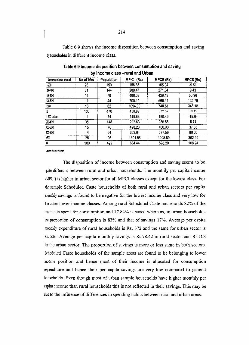
214
Table 6.9 shows the income disposition between consumption and saving
by households in different income class.
Table 6.9 Income disposition between consumption and saving by income class -rural and Urban
Income class rural Noofhhs Population MPC I (Rs) MPCE(Rs) 1·200 28 150 156.33 165.94 m400 31 144 280.47 271.04 lOO-6OO 14 70 486.09 429.13 m.800 11 44 700.19 565.41 >800 16 62 1094.99 748.81 ~ 100 470 451Jgg ':\7? f:07
1·200 urban 11 54 149.86 169.49 m.4OO 35 148 292.63 286.88 400-600 15 70 498.23 460.90 &)J.8()() 14 54 663.64 577.59 >800 25 96 1391.58 1028.59 All 100 422 634.44 526.20
Sooo:e: Survey data
MPCS (Rs) -9.61 9.43 56.96 134.79 346.18 7A tt?
-19.64 5.74 37.33 86.05 362.99 108.24
The disposition of income between consumption and saving seems to be
quite different between rural and urban households. The monthly per capita income
(MPCI) is higher in urban sector for all MPCI classes except for the lowest class. For
the sample Scheduled Caste households of both rural and urban sectors per capita
monthly savings is found to be negative for the lowest income class and very low for
the other lower income classes. Among rural Scheduled Caste households 82% of the
income is spent for consumption and 17.84% is saved where as, in urban households
the proportion of consumption is 83% and that of savings 17%. Average per capita
monthly expenditure of rural households is Rs. 372 and the same for urban sector is
Rs. 526. Average per capita monthly savings is Rs.78.42 in rural sector and Rs.108
for the urban sector. The proportion of savings is more or less same in both sectors.
Scheduled Caste households of the sample areas are found to be belonging to lower
income position and hence most of their income is allocated for consumption
expenditure and hence their per capita savings are very low compared to general
households. Even though most of urban sample households have higher monthly per
capita income than rural households this is not reflected in their savings. This may be
due to the influence of differences in spending habits between rural and urban areas.

215
6.1.9 Structure of houses
The general characteristics of a household like type of structure of houses,
facilities like electricity, drinking water etc., and ownership of land, outstanding
liabilities etc. give an idea about the standard of living of the study households. Table
6.10 gives the type of structure of sample Scheduled Caste households in the rural
and urban sector.
Table 6.10. Type of structure of houses (%)
iSLNo No. of Floor rooms
Wall Roof Ownership ,
Cow Coco. Wooden. Bricks. Bricks. Cooo. Any Mud Cement Mosaic Tiles non. Mud tiles Asbestos. Conaete Own dung Leaves Planks Plastered. I plastered Leaves other
Rum! 2.95 18 49 32 0 0 5 3 37 13 36 29 60 4 3 72 28
lhbir1 3.02 17 25 56 2 0 0 6 56 19 19 22 63 4 6 53 47
Source: Survey data
It is found that most of the sample households live in very low standard
houses both in rural and urban sector. In spite of the various types of housing aids
provided to Scheduled Castes by different schemes their housing condition has not
improved much for most of the households investigated. Average number of rooms in
rural is 2.95 where as it is only 3.02 in urban sector.
6.1.10 Household facilities
Table 6.11 shows the general facilities available to sample
households.22% of rural and 64% of urban sample households live in electrified
houses. 17% of rural and 13% in urban have their own wells. The average distance to
town is 18 kms in rural and 2.89 kms in urban area. While in rural area hospital
facility is available within a distance of 2 kms, in the urban area the average distance
to medical facility is only 0.86 km.
Table 6.11. General facilities available to sample households [% of households.]
Electrified Drinking water Average distance (km) houses to
Own well Neighbors Public tap Town School Hospital Rural 22 17 33 43 18 2.46 2 Urban 64 13 31 38 2.89 1.83 0.86
Source: Survey data

216
U.l1 Liabilities outstanding
Table 6.12 shows the outstanding liabilities of sample Scheduled Caste
households for five per capita expenditure classes (MPCE). 43% of rural and 27% of
urban sample households below MPCE of Rs. 400 depend on loans to meet their
basic requirements. As already seen the sample households are in a very low-income
position and so most of the households are in debt. 61 % of rural and 54% in urban are
in debt. It is observed that most of the households are in the grip of poverty. Poverty
not surprisingly, has its own culture, if it exists and has long existed, people come to
tenns with it. They cease to struggle against the obtrusively nonnal for seemingly
impossible11 •
Table 6.12 Outstanding Liabilities of sample households
MPCEClass No of households with Loan rural No of households with loan Urban
1).200 18 11
:200400 25 16
140().600 9 8
,6()0.8oo 4 8
>800 5 11
Total 61 54
Source: Survey data
6.1.12 Ownership of land
Table 6.13 shows the nature of ownership of land by Scheduled Castes.
Scheduled Castes in rural possess on an average 21.89 cents of land and in urban this is
8.22 cents. Land ownership of Scheduled Castes in the study area is very poor. Besides
own land some of them are in ' Kudikidappu', 'Purampokku' lands and some in 'othersI2 ,
Table 6.13 Land ownership pattern of sample households
Rural Urban (acrel Cents) (Acre! Cents)
I Own 21.89 8.22 i Kudukidappu 0.00 0.08 Purampokke 0.05 0.38 Others 0.21 0.11 Total 19.95 8.38
Source: Survey data

217
U Monthly per capita consumption expenditure
Expenditure-based indicator is used in most studies than income, as
oouseholds tend to hold back information on income, but found more open about
reporting real expenditure levelsl3• This is based on expenditures made by households
ID consume goods and services. Variations in income receipts and the inability or
IIDwillingness of survey respondents to report completely and accurately how much
IIICOme was received can cause income to be an unreliable measure of household
economic resources. Obviously, when consumer income is under stated, the consumer
unit can be classified as poor when it is not. Given these problems in measuring
income, researchers have used total expenditures as a proxy for income. The
theoretical basis for this substitution is the permanent income hypothesis. It suggests
that consumers try to maintain a given level of consumption over time and are
relatively unresponsive to transitory increases and decreases in income. Thus:
compared with measures of annual income, annual total expenditures are a better
representation of consumption patterns over the lifespan. One drawback of using total
expenditures instead of income when assessing household's economic status is that a
household might appear to be poor on the basis of total expenditures, when it is
simply saving rather than spending. To overcome .this drawback, it is suggested of
using total expenditures in addition to, rather than instead of, income when assessing
whether a household is above or below the poverty thresholds.
For a household, MPCE is household consumer expenditure over a period
of 30 days divided oy its household size. A person's MPCE is understood as that of
the household to which he belongs14. Table 6.14 gives distribution of sample
scheduled caste households over five classes of MPCE of the study area for rural and
urban sectors.

218
Table 6.14 Distribution of sample population based on MPCE ciasses
Monthly per capita Rural Urban
expenditure Percentage of % Of population Percentage of % Of population households Households
1·200 28 31.70 13 14.69
200-400 36 35.96 34 35.55
400-600 20 20.4J 20 19.19
600-800 10 7.45 17 16.11
>800 6 4.47 16 14.45
100 100 100 iGG I .~~
IVV
SaJce: Survey data
It may be observed that among the rural sample households 28% were
below the MPCE level of Rs. 200 compared to 1:;% for urban. Another 36% of
sample rural households were in the range of Rs. 200 - Rs. 400 along with 34% of
urban households. While 16% of sample urban households were above the MPCE
level of>Rs 800,only 6%ofthe rural population belonged to the highest MPCE class.
Considerable variation in the distribution of households by MPCE was
found in the two sectors. 28% of rural sample households and 13% in urban sample
households were in the lowest MPCE class. Number of households was highest in the
MPCE class of 200-400 in both rural and urban sectors. Number of households in the
highest MPCE class of>Rs.800 was 6 rural in and 16 in urban. Figure 6.1 shows the
distribution of population between MPCE classes for rural and urban sample areas.
Figure 6.1. Distribution of population between different MPCE classes
40r---------------------r===~
35
....... 30 ~ :.... 25 c o ~ 20
"[ 15 o a.. 10
5
o 0-200 200400 400-600 600-800 >800
MPCE Class
Source: Survey data
I

i , , ,
!
219
6.3 Average Monthly Per capita Consumption Expenditure
For general households -the all India rural average MPCE was Rs. 486 in
which Rs.288 was for food and Rs.187 for non-food as per NSSO 55th round [1999-
2000]. For urban it was Rs.854 of which Rs.410 for food and Rs.444 for non-food The
average MPCE in urban India exceeded average MPCE in rural by more than 60%.
In Kerala rural average MPCE was Rs. 766 of which Rs.411 was for food
and Rs. 354 for non-food. For urban this was Rs. 932 in which Rs.457 for food and
Rs.475 for non-food1s• The average MPCE in urban Kerala exceeded average MPCE
in rural Kerala by only 26%. For SC's as per NSSO 50th round data average MPCE in
rural All India was Rs. 238 and for urban Rs. 346. Average MPCE of Scheduled
castes for rural and urban sample areas are shown in Table.6.15
The average MPCE in the urban sector (Rs.526) exceeded the average
MPCE in the rural area (Rs.372). Average Urban MPCE exceeded average rural
MPCE by more than 30% for the sample SC popUlation. It is found that the in the
sample area SC's have a very low average MPCE.
a e . . verage T bl 615 A an verage MPCE dA h ouse 0 size h Id . Average household size Average MPCE
Rural 4.70 372
Urban 4.22 526
Soulte: survey data
Average MPCE on broad groups of food and non-food items for sample
se households per person for each MPCE class in the rural and urban areas are given
in Table 6.16.
Table 6.16 it is observed that there are wide rural and urban differences in
the proportion of expenditure on food and non-food items for most of the expenditure
classes. The proportion of non-food expenditure is higher for higher expenditure class
and lower for lower expenditure class in rural sector. Similarly the proportion of food
expenditure is higher for lower expenditure classes and lower for higher expenditure
classes in rural sector. While the lowest expenditure class in rural sector spend
64.30% of their MPCE on food items, the highest expenditure class spend only
47.75%of their MPCE on food. Like wise while the proportion of expenditure of non-
i

, ,
I
220
food of the lowest expenditure class is 35.70%, the highest expenditure class spend
52.25% of their MPCE on non-food items.
Table 6.16 Distribution of sample households by expenditure on food and
non-food items for various expenditure classes
MPCE class Rural No. of households
1-200
2Q0.400
400-600
600-800
>800
Urban
1-200
200-400
400-600
600-800
>800
(F~ures in brackets represent %.)
Source: Survey data.
28
36
20
10
6
13
34
20
17
16
Population %
31.70
35.96
20.43
7.45
4.47
14.69
35.55
19.19
16.11
14.45
MPCE MPCEon food
154.99 99.66 (100) (64.30)
285.62 179.4 (10Ql 162.7!ll
490.36 273.28 (100) (55.73)
691.63 365.2 (100) (52.85)
985.16 470.39 (10Ql 147.75)
167.30 88.81 (100) (53.08)
289.00 146.7 (100) (50.8)
483.63 238.75 (10Ql _149.37)
685.28 317.54 (100) (46.34)
1206.04 476.59 (100) (39.5~
MPCEon non-food
54.91 (35.70) 106.26
137.211 217.61 (44.27) 326.20 (47.15) 514.90
152.25)
78.24 (46.91) 142.81 (49.43) 244.05 (50.63) 367.81 (53.66) 730.67
160.48)
A similar pattern is observed in the urban sector also. We see that lower
expenditure classes spend more proportion of their tota] expenditure on food than
higher expenditure classes. Proportion of expenditure on non-food of higher
expenditure classes of urban sector is found much higher than the same of lower
expenditure classes in the urban sector.
In case of urban sector the lowest expenditure class spend 53.08% of their
MPCE on food items. The highest expenditure classes spend only 39.52% of their
MPCE on food items. The proportion of expenditure on non-food items of the lowest
expenditure class in the urban sector of 46.91 % is much less than the same of the
highest expenditure class in the urban sector (60.48%)

221
We find significant differences between rural Scheduled castes and urban
Scheduled castes in their distribution of MPCE between food and non-food items.
Considering the first expenditure class Rs.I-200 proportion of MPCE on food items
in the rural sector was 64.30% while that of urban sector is much lower 53.08%.
For the second expenditure class Rs. 200-400, the proportion of MPCE on
food items in the rural and urban sector were lower as 62.79% and 50.58%
respectively. For the third expenditure class Rs. 400-600, the proportion of MPCE on
food items in the rural sector is still lower as 55.73% and in the urban sector for the
same class it was 49.3 7%.
Considering the fourth expenditure class Rs. 600-800, in the rural sector
the proportion of MPCE on food items was only 52.85% and in the urban sector for
the same class it was 46.34%. Regarding the fifth expenditure class >Rs. 800, in the
rural sector the proportion of MPCE on food items was further lower as 47.75% to
while in the urban for the same class for food items it was 39.52. We find that both in
rural and urban sectors the proportion of MPCE on food items is declining as we
move from lower to higher expenditure classes.
It was found that the proportion of expenditure on non-food items
increased from lower to higher MPCE class in both rural and urban sector.
Considering non-food item in the consumption basket of sample SC households for
the first expenditure class Rs. 1-200 in the rural sector, the proportion of MPCE on
non-food items was 35.70% and the same for the same class in the urban sector, the
proportion of expenditure on non-food items was much higher 46.91 %. In the rural
sector for the second expenditure class Rs. 200-400 the proportion of MPCE on non
food items was 37.21 %. While in the urban sector for the same class the proportion of
MPCE on non-food items was 49.43%
For the third expenditure class in the rural sector Rs. 400-600 the
proportion of MPCE on non-food items was higher as 44.27% and in the urban sector
the MPCE on non-food items 50.63%. Regarding the fourth expenditure class Rs. 600-
800 in the rural sector the proportion ofMPCE on non-food item was 47.15% and in
the urban sector for the fourth expenditure class the corresponding MPCE was 53.66%.

222
In the fifth expenditure class > Rs.800, the proportion of MPCE on non
food items in the rural sector was 52.25% and corresponding MPCE in the same class
for urban sector was 60.48%.
Regarding non-food items moving from lower to higher expenditure class
the proportion of MPCE on non-food is increasing. The decline in the proportion of /
MPCE on food items for the urban sector is more pronounced than rural sector. The
increase in the proportion of MPCE on non-food items is more pronounced for urban
sector than rural sector. We find that the influence of place of residence is very
significant in the allocation ofivlPCE uu LUUU CU1U llUll-LUUU ii.c:ms by Scheduled castes.
6.4 Per capita expenditure on different items of consumption: Engel ratio Analysis.
The consumption pattern of Scheduled Caste households is analyzed by
studying the differences in the expenditure on different items in the consumption
baskets. The NSSO classifies expenditure into 33 items. Here for the present study
data on 25 items have been collected and presented. This includes 12 food items and
13 non-food items. Among the food items expenditure on cooked food purchased is
also included as a new item of expenditure. This is because we find a considerable
number of households reporting consumption of cooked food purchased. Table 6.17
presents the average MPCE and Engel ratio estimated from household consumption
data for rural an urban Scheduled Caste households. It attempts to examine the
differences in their expenditure on each of food and non-food items.
The break up of MPCE of sample Scheduled C~ste households is taken
for 25 groups that is 12 food groups and 13 non- food groups for the sample rural and
urban areas. The main features revealed by the survey data are as follows.
For the rural sector per capita 30 days consumer expenditure ofRs.372.57
was spilt up in to Rs. 211.90 on an average on food and Rs.160.67 for non-food. Food
constituted 56.88% and non-food 43.12 % of MPCE. Among food items Cereals
constituted 19.28 %, Meat, fish & egg 6.24 %, Vegetables 4.64 % and Fruits 4.62 %.
The Engel ratio for cooked food purchased was 6.79 %, for Spices 3.43 % and for
Milk & milk products only 2.62%.

lNo
1 2 3 4
5 6 7 8 9 10 11 12 13 14 15 16 17 18 19 20
21 22
23
24 25 26
27
28 29
30
223
Table 6.17. Average Monthly Expenditure per person on different items in the rural and urban areas
Rural Urban Item Average MPCE Engel Average MPCE
(Rs.) ratio (Rs.) Cereals 71.83 19.28 68.52
Pulses 5.71 1.53 7.81
Milk & milk products 9.74 2.62 19.28 I:dibleoil 12.36 3.32 16.31
~at, fish & egg 23.23 6.24 29.34
~egetables 17.3 4.64 17.93 ruits 17.19 4.62 21.99
~ugar 7.27 1.95 10.22
Beverages 7.77 2.09 11.74
Salts 1.42 0.38 1.37
Spices 12.78 3.43 14.01
Cooked food purchased 25.28 6.79 20.75 ~oodtotal 211.9 56.88 239.23
Pan, tobacco & intoxicants 40.31 10.82 45.84 uel & light 21.35 5.73 44.71
Clothing 21.19 5.69 29.2 Footwear 2.61 0.70 2.57
ducation 7.99 2.14 14.74 Medical 11 2.95 25.03 Entertainment 5.33 1.43 5.44 poods for personnel care 11.19 3.00 17.87
Piher mise. Goods. 11.83 3.17 16.03 ~isc.Consumer goods=20+21 +22 28.35 7.61 39.34
~ravel 9.71 2.61 14.24
~ent 0 0 0 Taxes 0.19 0.05 2.5 Mise. goods and 38.26 10.27 56.09 services=23+24+ 25+ 26 Durable goods 17.96 4.82 68.80 All non food total 160.67 43.12 286.97 .
otal consumer expenditure 372.57 100 526.2 lIUt8: Survey data
Engel ratio 13.02 1.48 3.66 3.10 5.57 3.41 4.18 1.94 2.23
0.26 2.66 3.94 45.5 8.71 8.5
5.55 0.49
2.8 4.76 1.03 3.4 3.05 7.48
2.71 0
0.48
10.7
13.1 54.5 100
Among non-food items, Engel ratio for Pan, tobacco & intoxicants alone
accounted to 10.82 %. Miscellaneous consumer goods includes entertainments,
Goods for personal care and effects, and other Miscellaneous goods. Here
expenditure on services such as Medical services and Education are given separately
and they are not included in Miscellaneous services. Miscellaneous services include
expenditure on Travel, Rent and Taxes.

224
Among non-food items Miscellaneous goods and services constituted
10.27 %. Per capita expenditure on services such as Education and Medical services
are given separately. While expenditure on Clothing and Footwear accounted 6.39 %,
Fuel & light constituted 5.73 %. Engel ratio for Durable goods was 4.82 %, and for
Education only 2.14 %.
For the urban sector average MPCE of Rs.526.20 was split up in to
Rs.239.23 for food and RS.208 for non-food expenditure. Food expenditure
constituted 45.5% and non-food, 54.5 % of MPCE in the urban sector. Engel ratio for
Cereals was 13.02 %, while for Meat, fish & egg was 5.57 %. Vegetables and Fruits
together accounted 7.59 % and Milk & milk products constituted 3.66 % of MPCE in
urban areas. For the urban sample expenditure on cooked food purchased from out
side constituted 3.94 %.
For the urban sector ~ong non-food items Pan, tobacco intoxicants alone
accounted to 8.71 %. Miscellaneous consumer goods includes as in case of rural,
entertainments, Goods for personal care and effects and other personal goods.
Expenditure on services such as Medical services and Education are given separately
they are not included in Miscellaneous services. Miscellaneous services include
expenditure on Travel, Rent, and Taxes.
Among non-food items Miscellaneous goods and servIces constituted
10.7 %. While expenditure on Clothing and Footwear together accounted to 6.04 %,
for Fuel & light it was 8.5 %. Expenditure for Durable goods accounted to 13.1 % of
MPCE in the urban sector and Engel ratio for Education was 2.8 %.
Rural Expenditure levels per capita did not exceeded urban levels for all
the item groups except Cereals and Salt.
6.5 Average Monthly Expenditure and Engel Ratios
Table 6.17 given earlier express estimated Engel ratios for all food and
non-food items for rural and urban sample. It may be noted that the Engel ratio for
food total (56.88%) is higher for rural sample and low for urban sample (Rs.45.46).

225
Regarding non-food items the Engel ratios of non-food total is higher in urban sample
(54.54) than rural sample (43.12).
The estimated values of Engel ratios given in the Table are compared for
rural and urban sample. Rural - urban differences in MPCE is pronounced in case of
certain items. Among food items Engel ratio on the items Cereals, Pulses, Edible oil,
Mea~ fish & egg, Vegetables, Fruits, Sugar, Salt, Spices and cooked food purchased,
rural expenditure exceeded urban. For the food items Milk & Milk products and
Beverages, urban expenditure exceeded rural. For the food items Cereals. Cooked food
and Vegetables rural expenditure is observed to be much higher than urban
expenditure.
Important rural urban differences are found in the share of Cereals, (rural
share exceeding urban by 6.26 % points. Households in urban sample spend more on
non-food items compared to households in rural sample. Among non-food items
Engel ratio on the items Pan, tobacco & intoxicants, Entertainments and footwear,
rural expenditure exceeded urban. For all other non-food items Scheduled Caste in
the urban sector spend higher than rural.
Urban Medical expenditure was higher by 127.5% than the same by rural
households. Regarding Education the urban area monthly per capita expenditure was
double than that of rural. It was found that rural expenditure 011 pan, tobacco
intoxicants (RsA0.31) was more or less closer to urban expenditure (RsA5.84) on the
same item. Non-food expenditure per person in the urban sector (2X(;.97) was 79%
higher than that in the rural sector (160.67).
Table 6.18 and 6.19 shows the rural urban differences in the share of food
and non-food items.

226
I Tables 6.18 Percentage Of MPCE on specific item groups: rural-urban differences. Rural share>urban share
SI. No Item group Rural Urban 1 Cereals 19.28 13.02 2 Pulses 1.53 1.48 3 Edible oil 3.32 3.10 4 Meat Fish & Egg 6.24 5.57 5 Vegetables 4.64 3.41
6 Fruits 4.62 4.18
7 Sugar 1.95 1.94
8 Salt 0.38 0.26
" "'-:--- 3.43 2.66 " vl"\N"
10 Cooked food purchased 6.79 3.94
11 Food Total 56.88 45.46 12 Pan, Tobacco intoxicates 10.82 8.71 13 Cioth 5.69 5.55 14 Footwear 0.70 0.49 15 Miscellaneous consumer goods 3.17 3.05
SoIIt8: Survey data
Table 6.19 Urban Share> Rural Share
Item group Rural Urban
t.ik & milk product 2.62 3.66
Beverages 2.09 2.23
Fuel & light 5.73 8.50
Education 2.14 2.80
f.'edical 2.95 4.76
Miscellaneous goods& Services 10.27 10.66
Durable goods 4.82 13.07
Soun:e: Survey data
Among food items the highest rural-urban difference is found for the item
Milk & milk products. Urban expenditure on the item is found higher by (Rs.9.5) than
rural Among non-food items the highest rural-urban difference is found for item
Durable goods. Average urban expenditure on the item is higher by (Rs.50.84) than
rural sector.
An F-test was carried out to fined out if there is a significant difference
between rural and urban areas with respect to total expenditure, expenditure on food
and expenditure on non-food. The results are given in Table 6.20.

227
Table 6.20. Results of 'F' test
Items Group
0IaI expenditure Rural Urban
food total Rural Urban
~food Rural Urban
• $Vnificant at 1 % level, ns - non signifICant at 5 % level Slrveydata
Mean Expenditure 372.5672 526.1990 211.9012 239.2287 160.6660 286.9703
F - value
12.2**
2.0Ons
19.433**
Significant F-value indicates that the mean consumption is different for
Rural and urban. In the case of food consumption, there is no significant difference in
the mean consumption between two groups (rural and urban). Total expenditure is
significantly higher in the urban group compared to rural group. Similarly non-food
consumption was also higher in urban area. F value is founded significant in the case
oftotal expenditure. The calculated value of F is 12.2 while tabled value of F at 1 %
level of significance is 3.5 Hence the difference is significant.
In the case of food items however the calculated F value is 2, which is
found to be non- significant. Hence there is no significant difference between the
rural and urban areas as far as food expenditure is concerned. On the contrary for
non-food items the calculated value of F is equal to 19.433, the difference is
significant at 1 % level.
6.6 Percentage expenditure of each food item in total food expenditure and
percentage expenditure of each non -food item in total non-food expenditures.
Table 6.21 gives % of selected items of food in total food expenditure in
rural and urban areas. Among food item sample rural SC households spend the
highest % of 33.90 on Cereals while this is 28.64% in urban. Expenditure on cooked
food purchased constitute 11.93% of total food expenditure in rural area and 8.67% in
urban. Rural Scheduled castes spend 11 % of their average MPCE on Meat, fish, and
egg and urban Scheduled castes spend 12.26%. Other food items attracting more
expenditure in both rural and urban are Vegetables, Fruits and Spices and Edible oil.
Expenditure on Milk & milk products constitute 4.60% of total food expenditure and
8.04 % in urban sector.

228
Figures 6.2 and 6.3 gives % expenditure on selected item of food to total
food and % expenditure on selected item of non -food to total non- food expenditure.
Among the non-food items Pan, tobacco & intoxicants had the highest share in rural
areas (2S.09%). In urban areas too it come up to 15.97.
T bl 621 P a e .• ercentage E xpen d' I t d't ff dt Iture on se ec e lemso 00 otota If d 00 expen
Items % Expenditure
Rural Urban (Meals 33.90 28.64
Pulses 2.70 3.26
~ & milk products 4.60 8.04 Edible oil 5.84 6.82
Meal, fish & egg 10.96 12.26
Vegetables 8.17 7.50 Fruits 8.11 9.19
&igar 3.43 4.27
Beverages 3.67 4.91
Salt 0.67 0.57
~ 6.03 5.86
~ed food purchased 11.93 8.67 Food total 100.00 100.00
Source: Survey data
Figure 6.2. Percentage expenditure on selected item of food to
total food expenditure in rural and urban areas
60
50
GI 40 .. ::I ..
iD Rural
I Cl Urban :c 30 c 11 Q,
Ll1 20
10
0 'i ~ 'i! c:> .. ill .":
~ ~ ~ .. ~ u ~ .= :: ~
.. .= fO: C J
"
:i .. i Oil "i Cl ill QAI ~
~ ! :£ " tIl :I .. ~ ill tIl ~ tIl QAI
~ ill
:=
~ ~ :: ~
source: survay data
All
31.11
3.00 6.42 6.36
11.65 7.81
8.69 3.88 4.32
0.62 5.94
10.20 100
; .. !
d't lure

229
Table. 6.22. Percentage Expenditure on selected items of non-food to I f d d't tota non· 00 expen lures
.I
% Expenditure Items
Rural Urban All _ & intoxicants 25.09 15.97 19.25 I
IlIiIJ! 13.29 15.58 14.76
~ 13.19 10.17 11.26
~ 1.62 0.89 1.16
~ 4.97 5.14 5.08 I
la 6.84 8.72 8.05 ! IIII1eIIt 3.32 1.90 2.41
Ilrl8SOl1nel care O:;j/ 6.23 6.49 i • 7.36 5.59 6.22
I :JISUfJ1ergoods 17.64 13.71 15.12
'. 6.05 496 5.35
0.00 0.00 0.00 I I 0.12 0.87 0.60 I
JD1s and services 23.81 19.54 21.08 , ~pxls 11.18 23.97 19.38
~blj total 100 100 100 ~inttDaIa
Figure 6.3, Percentage expenditure on selected item of non-food to total non·food expenditure in rural and urban areas
&l
50 I I
ID Rural I,~
1111 Urban • : :l)
: " !l
,
: rI rlI na r-filrlI...,. r1iJ rm r1i1iI r ~ - QI) L. C
" - ~ c i '" 1 " ..c c " 0 C L. .2 ~ c ~ :s £ ;: ~
~ " " ~ 'S 11 =a ~ - ~ ~ " .8 ~ -- QI)
i "Cl 0
l ~ i c 'ii 'B c 0 j '" c 1: ~ .s .. " - 0 - l5 .: 'ii L.
'" C " ~ L. a L. c -= tf - a :::I
Q
C &; Q 2: 11 L. 0 .s ~
.! J :I .. C 11
A-
i
i imeydata

230
6.7 Engel ratio at the disaggregate level for comparable expenditure classes
Consumption expenditure pattern of Scheduled caste households in the
rural and urban sample areas belonging to different comparable monthly per capita
consumption expenditure classes are presented in this section. The estimated Engel
ratio on each food and non-food items is used for comparing the consumption
expenditure pattern of households belonging to comparable MPCE class in rural and
urban sectors. Differen~es if any between rural and urban households will show that
the influence of place of residence on household's consumption pattern.
Table 6.23. Gives the average MPCE on broad groups of food and non
food items per person for a period of 30 days for each MPCE class of rural and Table
6.24 the same for urban sample.

11
....
... _
-
-1
-20
0-
%
200~---~
.C:J
ooU
_C!>
CM
.t
Cerea
ls
48
.67
2
9.0
9
53
.79
1
8.6
1
72
.51
Pul
ses
1.7
4
1.0
4
3.1
2
1.0
ft
7.3
1
Mil
k &
m
ilk
prod
ucts
0.
14
0.08
5.
62
1.94
15
.48
Edi
ble
oil
4.52
2.
70
9.48
3.
28
16.4
4
Mea
t, f
ish
& e
gg
4.79
2.
87
15.2
3 5.
27
33.4
6
Veg
elab
les
5.04
3.
01
9.03
3
.\3
13
.32
Fru
its
7.90
4.
72
9.72
3.
36
21.9
8
Sug
ar
5.66
3.
38
7.46
2.
58
10.9
0
Bev
erag
es
1.61
0.
96
6.87
2.
38
11.8
6
Sal
t 0.
99
0.59
1.
39
0.48
1.
60
Spi
ces
5.81
3.
47
7.76
2.
69
14.0
9
Hot
el
1.95
1.
16
16.7
0 5.
78
19.8
1
Foo
d to
lal
88.8
1 53
.08
146.
17
50.5
8 23
8.75
Pan
, tub
aco
and
into
xica
nts
12.4
1 7.
42
41.1
3 14
.23
61.3
3
Fuel
and
lig
ht
30.1
3 18
.01
39.2
1 13
.57
50.7
9
Clo
thin
g 6.
71
4.01
12
.57
4.35
24
.88
Foo
twea
r 0.
57
0.34
0.
99
0.34
2.
31
Edu
cati
on
2.07
1.
24
7.32
2.
53
9.48
Med
ical
9.
51
5.68
14
.74
5.10
22
.43
Ent
erJa
inrn
ent
0.97
0.
58
2.11
0.
73
2.87
Goo
ds f
or p
erso
nnel
car
e 5.
16
3.09
10
.04
3.47
18
.14
Con
trib
utio
n 2.
03
1.21
3.
94
1.36
4.
45
Mis
e. c
onsu
mer
goo
ds =
20+
21 +
22
8.16
4.
88
16.0
9 5.
57
25.4
7
Tra
vel
2.08
. 1
.25
4.61
1.
60
6.43
Ren
t 0.
00
0.00
0.
00
0.00
0.
00
Tax
es
0.08
0.
05
0.00
0.
00
0.31
Mis
e. g
oods
and
ser
vice
s= 2
3+24
+25
+26
10
.32
6.17
20
.71
7.16
32
.21
Dur
able
goo
ds
6.51
4.
04
6.15
2.
14
40.6
3
All
non
food
tol
al
78.2
4 46
.91
142.
81
49.4
3 24
4.05
Tol
al c
onsu
mer
exp
endi
ture
16
7.30
10
0.00
28
9.00
10
0.00
48
3.63
"'. -.:
: ..
.. _-
---
~-""K)
--f
l.c.c
.t
14
.99
8
3.6
2
12
.20
9
4.9
0
1.5
1
10
.92
1
.5')
2
0.0
2
3.20
21
.18
3.09
66
.35
3.40
22
.18
3.24
34
.01
6.92
38
.57
5.63
64
.27
2.75
29
.13
4.25
41
.19
4.54
30
.21
4.41
50
.83
2.25
11
.98
1.75
17
.06
2.45
16
.61
2.42
25
.01
0.33
1.
25
0.18
1.
49
2.91
17
.24
2.52
30
.45
4.10
34
.67
5.06
31
.02
4}.3
7 31
7.54
46
.34
476.
59
12.6
8 58
.35
8.51
50
.38
10.5
0 46
.16
6.74
59
.08
5.14
38
.27
5.58
78
.56
0.48
2.
86
0.42
7.
55
1.96
23
.45
3.42
38
.14
4.64
51
.20
7.47
34
.95
0.59
7.
07
1.03
17
.63
3.75
22
.85
3.33
39
.19
0.92
11
.88
1.73
71
.99
5 .. "1
7 41
.79
6.10
12
8.81
1.33
10
.98
1.60
57
.83
0.00
0.
00
0.00
0.
00
0.06
1.
35
0.20
13
.75
6.66
54
.11
7.90
20
0.38
8.57
93
.40
13.6
2 26
1.62
50.6
3 36
7.81
53
.66
730.
67
100.
00
685.
28
100.
00
1206
.04
-7
.87
6
11
. .5
2
1.6
c.
7.8
\
5.50
\9
.24
2.82
16
.31
5.33
29
.34
3.42
17
.93
4.21
21
.99
1.41
10
.22
2.07
11
.74
0.12
1.
37
2.52
14
.01
2.57
20
.75
39.5
2 23
9.23
4.18
45
.84
4.90
44
.71
6.51
29
.20
0.63
2.
57
3.16
14
.74
2.90
25
.03
1.46
5.
44
3.25
17
.87
5.97
16
.03
10.6
8 39
.34
4.79
14
.24
0.00
0.
00
1.14
2.
50
16.6
2 56
.08
21.5
9 68
.80
60.4
8 28
6.97
100.
00
526.
20 ~ ..
13
02
l.4
K
3.(
,{)
3.10
--
5.57
3.41
-.-
4.1H
-
1.94
2.23
0.26
2.66
3.94
45.4
6
8.71
8.50
5.55
0.49
2.80
4.76
1.03
3.40
3.05
7.48
2.71
0.00
0.48
10.6
6
13.0
7
54.5
4
100.
00
N
W

---
.~ ...
.:-•
• -....
:-_-:,~~Ir .. -_ .
......
. ~~_.
-~-~--_ -
.... :.
..--
:~!1
, .... t.
~!.:'ft., ..
.. -.
IIC
I1'1
.-.1
1·2
(X)
'Yv
20
0-4
()()
0
/.
40
0-6
00
....
60
0-1
10
0
Cer
eals
53
.11
34.2
6 69
-45
24.3
2 84
.01
17.1
3 10
3.90
P
ulse
s 2.
03
1.31
4.
66
1.63
7.
67
1.56
9.
44
Mil
k &
mil
k pr
oduc
ts
2.42
1.
56
6.82
2.
39
16.8
6 3.
44
7.75
E
dibl
e oi
l 6.
49
4.18
11
.10
3.89
13
.27
2.71
18
.95
Mea
t, fi
sh &
egg
7.
59
4.90
19
.04
6.67
31
.93
6.51
38
.16
Veg
etab
les
6.33
4.
09
11.6
7 4.
08
29.1
6 5.
95
29.9
0
Fru
its
5.70
3.
68
16.2
3 5.
68
21.3
8 4.
36
19.0
3
Sug
ar
3.63
2.
34
6.75
2.
36
8.04
1.
64
13.6
1
Bev
erag
es
3.22
2.
08
6.\
3
2.15
11
.65
2.38
13
.62
Sal
t 1.
05
0.67
1.
31
0.46
1.
91
0.39
1.
49
Spi
ces
6.11
3.
94
13.5
5 4.
74
13.6
7 2.
79
17.8
9
Coo
ked
food
pur
chas
ed
1.99
1.
28
12.6
3 4.
42
33.7
3 6.
88
91.7
8
Food
tot
al
99.6
6 64
.30
179.
34
62.7
9 27
3.28
55
.73
365.
52
Pan
, tub
aco
and
into
xica
nts
17.8
6 11
.52
31.3
0 10
.96
41.2
8 8.
42
81.4
9
Fuel
and
lig
ht
15.3
0 9.
87
18.5
1 6.
48
22.0
5 4.
50
30.5
0 C
loth
ing
7.40
4.
78
16.5
4 5.
79
27.3
4 5.
58
32.8
0
Foo
twea
r 0.
65
0.42
1.
80
0.63
4.
37
0.89
4.
31
-E
duca
tion
3.
84
2.48
3.
54
1.24
14
.32
2.92
13
.18
Med
ical
2.
84
1.84
6.
89
2.41
11
.89
2.43
41
.93
Ent
erta
inm
ent
1.02
0.
66
2.04
0.
71
8.11
1.
65
12.1
7
Goo
ds f
or p
er. c
are
4.08
2.
63
8.32
2.
91
16.3
8 3.
34
19.\
3
Con
trib
utio
n 0.
66
0.43
6.
08
2.13
27
.65
5.64
9.
44
Mis
e. c
onsu
mer
goo
ds=
20+
21+
22
5.76
3.
71
16.4
4 5.
76
52.1
4 10
.63
40.7
4
Tra
vel
1.05
0.
68
4.40
1.
54
19,\
2 3.
90
16.5
9
Ren
t 0.
00
0.00
0.
00
0.00
0.
00
0.00
0.
00
Tax
es
0.00
0.
00
0.13
0.
05
0.62
0.
13
0.00
M
ise.
goo
ds a
nd
6.81
4.
39
20.9
7 7.
34
71.8
7 14
.66
57.3
3 se
rvie
es=
23+
24+
25+
26
Dur
able
goo
ds
0.21
0.
40
6.71
2.
36
24.4
8 4.
88
58.6
5
Al1
non
foo
d 54
.91
35.7
0 10
6.26
37
.21
217.
61
44.2
7 32
6.20
Tot
al c
onsu
mer
exp
endi
ture
15
4.99
10
0.00
28
5.62
10
0.00
49
0.36
10
0.00
69
1.63
-------" -
---
%
=.-
----
---
-. -
>1
10
0
'Ht
15.0
2 79
.37
8.06
71
.83
1.36
16
.49
1.67
5.
71
\.12
4
\.1
2
4.17
9.
74
2.74
33
.36
3.39
12
.36
5.52
67
.53
6.86
23
.23
4.32
41
.81
4.24
17
.30
2.75
59
.64
6.05
1
7.\
9
\.97
14
.29
1.45
7.
27
1.97
16
.\3
1.64
7.
77
0.22
2.
01
0.20
1.
42
2.59
27
.82
2.82
12
.78
13.2
7 70
.83
7.19
25
.28
52.8
5 47
0.39
47
.75
211.
90
12.6
5 11
7.29
11
.91
40.3
1
4.41
49
.01
4.97
21
.35
4.74
73
.63
7.47
21
.19
0.62
7.
90
0.80
2.
61
1.91
24
.31
2.47
7.
99
6.06
19
.16
1.94
11
.00
1.76
24
.51
2.49
5.
33
2.77
31
.09
3.\
6
11.1
9
1.37
49
.67
5.04
11
.83
5.89
10
5.27
10
.69
28.3
5
2.40
39
.23
3.98
9.
71
0.00
0.
00
0.00
0.
00
0.00
0.
38
0.04
0.
19
8.29
14
4.88
14
.71
38.2
6
8.47
78
.74
7.98
17
.96
47.1
5 51
4.90
52
.25
160.
67
100.
00
985.
16
100.
00
372.
57
._
.
All
19.2
8 1.
53
2.62
3.32
6.24
4.64
4.62
1.95
2.09
0.38
3.43
6.79
56.8
8
10.8
2
5.73
5.69
0.70
2.14
2.95
1.43
3.00
3.17
7.61
2.61
0.00
0.05
10.2
7
4.82
43
,\2
100.
00
N
VJ
I~
233
Average MPCE for five expenditure classes separately for each item of
5pCIlditure and for the aggregate rural sample and urban sample are presented in the
;.,Ic. Engel ratio for comparable expenditure classes of rural and urban sample is
lIIlpared here between rural and urban households.
In the lowest MPCE class Rs.1-200, among food items the estimated
:ngel ratios are found to be the lower for urban households for the items Cereals,
~Ises, Milk & milk products, Edible oil, meat, ilsh, and egg, Vegetables, Beverages,
~t and Spices and higher for Fruits, Sugar and expenditure on cooked food
lIIChased.
Among non-food items, the Engel ratio is found lower in urban
amcholds for the items Fuel & light, Medical expenses, Goods for personal care,
Travel, Taxes and Durable goods. It is found that between households belonging to
i3IIle expenditure classes in rural and urban there are significant differences in the
expenditure pattern especially in case of non-food items.
In the second MPCE class Rs.200-400, Engel ratios are found to be higher
in the rural sector for the food items, Cereals Milk & milk products, Edible oil, Meat,
fish & egg, Vegetables, Fruits, Spices and expenditure on cooked food purchase. The
UIban households of the same MPCE classes have higher Engel ratio for the items
Sugar, Beverages, and Salt.
Among non-food items expenditure is higher for rural households f0r the
items Clothing, Footwear and Durable goods. For the items Pan, tobacco &
intoxicants, Fuel & light, Education Medical expenses, expenditure on Entertainment,
and Goods for personal care and effects, Engel ratio for urban households are found
bigh. It is found that regarding consumption of almost all food items, place of
residence does not have much influence. But regarding non-food items the difference
between rural and urban households in Engel ratio is much higher and this shows for
this MPCE class of households. Thus it is found that urban households have more
preference to wards spending on non-food items even among Scheduled caste
households as similar to the case of general households in Kerala as per NSSO data.
234
Considering the third MPCE class Rs.400-600 estimated Engel ratios are
iIDI to be higher among the food items for rural households for the items Cereals,
~ Milk & milk products Vegetables and expenditure on cooked food purchased.
jpenditure of urban sample Scheduled caste households estimated Engel ratios were
oond higher for the food items Edible oil, Meat, fish & egg, Fruits, Sugar,
;."ierages, Salt and Spices.
Among non-food items Engel ratio is higher for urban households on the
ICIIlS pan, tobacco, Fuel & light. Rural households had higher Engel ratio only on
))II-food items such as Clothing Footwear, Education, Entertainment and travels.
We find that as we are moving to ward higher MPCE class, even for
:wJy of the food items like Beverages meat, fish, and egg urban households reported
:~er Engel ratios. In the urban sector expenditure on non-food is found to be
Rgnificantly different from rural expenditure.
In the next expenditure class Engel ratio is found to be significantly
~~er for rural sample households among food items only on items such as Cereals,
mdexpenditure on cooked food purchased. Regarding non-food items Engel ratio for
~ie items pan, tobacco& intoxicants and Travel were found significantly higher for
"Jl31 households.
Urban sample households Engel ratio of expenditure on non-food item
ruch as Fuel & light, Clothing, Education, Goods for personal care and Durable goods
lere found much higher than the rural sample households. It is found that for the
m,an upper MPCE class, non-food expenditure is significantly higher than other
i3/IIpJe househoJds. This is similar to what is revealed through NSSO data over the
period from 1983-2000 for Kerala.
For the highest expenditure class >Rs.800 it is found that expenditure on
iood items like Cereals constituting very smaller proportion of average MPCE as
compared to previous MPCE classes in both rural and urban sectors. In rural upper
MPCE class sample Scheduled caste households Engel ratios for the food items

235
:. Meat, fish & egg, Edible oil and cooked food purchased are found to be
iPficantly higher than urban.
It is found that rural Scheduled caste households in the upper MPCE
llges shows more preference towards nutritious food items such as meat fish & egg,
llIble oil, Fruits etc. Expenditure on purchased cooked food is found common
IOOng all classes of rural Scheduled caste households and high among higher MPCE
::asses of rural Scheduled caste households. For the lower MPCE classes this
.cy is found to be influenced by their particular occupation status. In the rural
mar most of them being agricultural labourers and other labourers they have to be
rtlY from their home for most of the day. They depend on the food available in the
lUls during especially in noon. But for the upper MPCE classes this may be viewed
Ea part of increasing preference towards imitation of general consumption pattern of
rt affiuent sections in Kerala - a tendency increasingly observed in the consumption
:memofKerala households - in recent years.
Regarding non-food items it is found that expenditure on Pan, tobacco &
jOxicants is higher for all MPCE classes in both rural and urban. The Engel ratio for
~ item is found much higher for upper MPCE classes of rural sample. For the rural
iiII1ple for the non-food items Clothing and Footwear and Entertainment also Engel
:lIio is found to be significantly higher than urban sector. Urban non-food items such
li Education, Goods for personal car~ & effects, Travel and Durable goods showed
~gher Engel ratio than rural households.
A very important observation is that while upper MPCE households of
.:ban sample show conspicuous consumption of Durable goods, Travel Goods for
:crsonal care & effects, Education etc, those of rural sector show similar consumption
~em for items such as pan, tobacco& intoxicants, Clothing, Footwear and
~lertainments. Besides the variable geographical factor has got significant influence
lD consumption pattern of Scheduled castes and rural urban differences are found to
:.emuch prominent regarding non-food expenditure.

I
236
~ Elasticity of Consumption Expenditure
r Regression Analysis
i In this section regression analysis has been used to find out the relation
expenditure on each food and non-food items and total expenditure of
le households. Among the many alternative forms available the following
. cations are tried; Linear, double log, log inverse and f<?r rural and urban
le. Among them Double log and Log inverse forms are presented here. The
for the other two forms; Linear and Log log inverse forms are given in
~models used are;
b. Double log: 10gEij = a. + PlogEj +u j
c. LogInverse: 10gEij =a+p(1fEj )+uj
1 d. Log-log Inverse: 10gEij =a+ PlogEj +r-+Uj
Ej
Where Eij is the MPCE of the ith item by /h household Ej is the total I 'P1thly per capita expenditure of /h household. <1, P and r shows parameters to be
'5limated and u is the random disturbance term.
11.8.1.1 Estimates using Double Log function
Table 6.25 and 6.26 presents regression analysis results using double log
'lIOdel for rural and urban sample SC households. The model is estimated using
ldinary least squares [OLS]100 households in rural and 100 households in urban are
i ased in the two Tables.
Expenditure elasticity has been estimated. The calculated values of P
Iq)resented as ~ in each equation shows expenditure elasticity. Estimates for each
'dern offood and non- food (24 items: 12 food and 12 non-food) are presented. For
loth rural and urban sample.

237
~ is found to be statistically significant at 1 % level for Cereals, Pulses,
jblc oil, Meat, fish & egg, Fruits, Sugar, Beverages, Spices, pan, tobacco, &
zlicants, Fuel & light, Clothing, Footwear, Education, Medical, Entertainment,
::avcl, Goods for personal care and Durable goods and at 5% level of significance
~thc items, Milk & milk products, Vegetables, Salt, and cooked food purchased.
In the rural sample among food items the highest elasticity is for the
:IfICIlditure on cooked food, the next being Vegetables. Other items with high
ilsticity are Meat, fish & egg (0.9979), Beverages (0.8936), Fruits (0.8204) and
jUblc oil (0.8195). Cereals being a necessary item the elasticity of Cereals 0.3170. It
sfound to be the second lowest among food items next to Salt (0.2520).
Table 6.25 Consumption pattern of rural households Estimated regression model: 10gEij = a + PlogEj + U j
Items a. p i.nIs 2.3718 0.3170 ~as -3.1918 0.8638 Ii & milk products -0.8259 0.6304 !ileoil -2.4020 0.8195 il,fish & egg -2.9338 0.9979 ~ -3.2438 1.0017 ;"As -2.1232 0.8204 s.gr -2.1768 0.6897 mges -3.3387 0.8936 ~ -1.2613 0.2520
= -1.6392 0.6987 ~ food purchased -3.5945 1.2163 1!1. klbacco & intoxicants -1.4558 0.8078 :.eI&I~ht 0.4378 0.4339 - -3.7835 1.1317 _r
-5.8929 1.1314 W:ation -4.0914 1.0876 IiXaI -4.0868 1.0323 ~ninment -3.0035 0.8598 '1IeI -7.3259 1.5987 GDIs for personal care -3.6671 1.0043 D.IIJIe~oods -7.6968 1.6893 'iqbl\ at 5% level; •• significant at 1 % level; ns - no significant iw: Survey data
SE (P) t- value
0.0590 55.377*" 0.1213 7.121** 0.2802 2.25" 0.0703 11.657** 0.1204 8.290** 0.1208 8.290" 0.1136 7.225** 0.0733 9.405** 0.0868 10.297** 0.1098 2.296* 0.0826 8.462** 0.2025 6.008" 0.1699 4.753** 0.0698 6.215** 0.0801 14.122*" 0.1172 9.655** 0.1455 7.477** 0.1653 6.247** 0.2437 3.529 .... 0.1884 8.484** 0.1032 9.731** 0.5315 3.178**
R2
0.4773 0.6563 0.3600 0.7622 0.6559 0.6559 0.6059 0.6888 0.7281 0.2472 0.6517 0.7027 0.4479 0.5317 0.8188 0.7212 0.7006 0.5702 0.4968 0.7357 0.7065 0.4403
While items such as expenditure on cooked food purchased constitute the
lIOS! lUXUry item among food items Vegetables, Meat, fish & egg, Beverages are also
iuxurious items in the food basket of rural SC households.

238
Among non-food items expenditure elasticity is lowest for the item Fuel
iltight (0.4339) and next Pan, tobacco &. intoxicants (0.8078) for rural sample se I
'uholds.
Expenditure elasticity is found to be highest for the items Durable goods
i1»893) and next Travel (1.5987). Other non-food items with higher expenditure
'2Iticity are Clothing, Footwear, Education, Medical expenses and Goods for personal
:Rand effects. Expenditure on Entertainment also has higher expenditure elasticity
We find that for the rural se households of the samnle area non-food
I lIDS Fuel & light and pan, tobacco& intoxicants are necessary items and other items
IEh as Clothing, Footwear, Education, Medical expenses and Goods for personal
zand effects are luxurious items of consumption.
Estimated Double log regression model for urban sample is given in
lable6.26
Table 6.26 Consumption pattern of urban households Estimated regression model: logEij =a+ PlogEj +uj
Items A
~ a. ~ 1.8659 0.3772 Nses -3.7211 0.9287 I & milk products -2.6748 0.9635 Etieoil -3.2782 0.9609 lilt fish & egg -4.6048 1.2489 It;IelalJles -3.8619 1.0682 IW -3.5681 1.0442 .. -1.1756 0.5491 tMrages -3.1065 0.8716 r.l -1.0464 0.2072 ~ -3.2327 0.9258 * food purchased 1.5684 0.3053 fit, IObacco & intoxicants 0.8058 0.4617 f.el&I~ht 1.5929 0.3460 D*I~g -4.4578 1.2288 foctrrear -5.1592 0.9673 fU:alion -3.4263 1.0050 IeXaI -2.0431 0.8058 ~nment -3.1950 0.8737 llMl -5.9223 1.3294 IiDIs for personal care -3.1533 0.9450 DnbIegoods -12.5772 2.4521 ,. .et •• .. span! at 5% levet, SignifICant at 1 % level, ns - no Significant
iw: Survey data
SE(~ ) t- value R2
0.0483 7.814** 0.6196 0.1086 8.552** 0.7099 0.1542 6.247** 0.6983 0.0636 15.100** 0.8376 0.0983 12.712** 0.7936 0.0858 12.453** 0.7971
. 0.6897 11.647** 0.7685 0.0757 7.253** 0.5910 0.1061 8.216** 0.6568 0.0800 2.59* 0.2607 0.0731 12.668** . 0.7879 0.1792 1.703ns 0.2436 0.1294 3.568** 0.3521 0.0666 5.196** 0.4648 0.0745 16.483** 0.8608 0.1198 8.074** 0.6868 0.1901 5.287** 0.5770 0.1712 4.706** . 0.4611 0.1746 5.004** 0.6458 0.1858 7.157** 0.6817 0.0871 10.846** 0.7403 0.3719 6.593** 0.6007

239
Among food items the elasticity is found to be low for Salt (0.2072),
eI food purchased (0.3053), Cereals (0.3772) and Sugar (0.5491). Among food
lIISbighest elasticity of expenditure is for Meat, fish & egg (1.2489). Other items
:iI higher expenditureelasticities are Vegetables, Fruits, Milk & milk products,
:ble oil, Spices, Pulses, and Beverages.
We find that in the urban sector also Cereals form a basic necessary item
:expenditure for the sample area. Other necessary items are Sugar, Salt, cooked
00 purchased.
Urban Scheduled caste households consider Meat, fish & egg as the most
mous items among food items. Other luxurious items are Vegetables, Fruits, Milk
tmilk products, Edible oil, Pulses, Spices and Beverages.
For the urban are among non-food items expenditure elasticity is lowest
~the item Fuel & light (0.3416). Items like Pan, tobacco & intoxicants (0.4617) also
11 low elasticity of expenditure compared to other non-food items for urban sample
iC households. Highest expenditure elasticity is found for the items Durable goods
~.4521) and the next highest Travel (1.3294). Other items with higher elasticities are
Jothing (1.2288) and Education (1.0050). Goods for personal care (0.9450),
:ootwear (0.9673) and Entertainment (0.8737) h~ve comparatively lower elasticity of
~penditure compared other non-food items for urban sector households.
It is found that for the urban sample households also the non-food items
fuel & light, and Pan, tobacco & intoxicants form the basic necessary items of
expenditure. For them the expenditure on Durable goods forms the most luxurious
item expenditure. Expenditure on Travel, Clothing, and Education are also luxurious
rtems in the expenditure list of SC's in urban sector. Urban SC's do not consider
purchase of Footwear and Goods for personal care and effects and expenditure on
Entertainment to be luxurious expenditure.
~8.1.2 Rural- Urban differences for food items
For both rural and urban sample households, Cereals form the basic
necessary item of consumption. It is found that the elasticity of expenditure on
Cereals is higher for urban sector compared to rural sector.

240
While expenditure on the cooked food purchased is a lUxury items in rural
Dple it is found as a necessary item in urban sample. Expenditure on Sugar is a
IIIIY item for rural households while the same is a necessary item for urban SC
aseholds. Meat, fish & egg fonns a lUXUry good for both rural and urban
IJSeholds but the elasticity of expenditure for the item is higher for urban sector.
r the rural sector elasticity of expenditure for Vegetables is higher than that for
!:at, fish & egg, the same is lower than that for Meat, fish & egg in urban sector.
:ban sector sample households are showing a preference towards Vegetables
,illpiln:u LU lilt; llt;.lU lVlt;(1l, U:;il & t:gg than rural households.
Milk & milk products have higher elasticity of expenditure in the urban
~rwhile it is lower for rural sample Scheduled caste households. The item is more
::a necessary one in the food basket of rural Scheduled castes. This may be mainly
~e of the share of consumption out of home grown stock in the rural sector.
Beverages fonn a luxury item for the rural and urban Scheduled castes.
jut the elasticity of the item to total expenditure is found to be higher for urban sector
Tan rural sector. Urban households show more preference towards the item compared
~rural SC's.
!.B.1.3 Rural- Urban differences for non-food items.
Elasticity of expenditure for non-food shows that Fuel & light and fan,
iDbacco & intoxicants are basic necessary items of consumption for both rural and
urban Scheduled caste households. Elasticity of expenditure for Fuel & light is higher
iorrural sector than urban sector.
One important observation regarding the sample SC households in the
study area is that Pan, tobacco & intoxicants is a less elastic item of non-food
expenditure in both rural and urban sample. SC popUlation of the sample area
regardless of rural and urban consider it as a basic necessary item of non-food. The
elasticity of expenditure for the item is low for the urban sector compared to rural
sector. For urban sector SC households, the elasticity of expenditure on Pan, tobacco
& intoxicants is closer to that of expenditure on Cereals.

241
Expenditure on Durable goods is considered a luxurious consumption by
] both rural and urban sector. The elasticity of expenditure on the item is found
dor urban sector somewhat double than that of rural sector. The item Goods for
;naI care showed higher expenditure elasticity in rural than urban. Households in
.sample show more preference towards consumption of the item than rural.
Entertainment expenditure has shown lower expenditure elasticity m
il sector than rural sector. Urban households show more preference towards
!!ling on Entertainment than rural households. Travel expenditure has shown
JeS of a lUXUry good both for rural and urban. The elasticity for the item is found
~forrural than urban sample.
Clothing expenditure has shown lower expenditure elasticity in urban
~than rural sector. But the difference is not as high as observed in case of other
:-food items. Expenditure on Footwear showed that the elasticity of expenditure on
l item is much lower in urban than the same in rural sector. To the urban
:tSCholds it is more of a necessary good compared to rural. Education expenditures
~e shown higher expenditure elasticity in rural than urban. In case of expenditure
: medicals, urban households have lower expenditure elasticity than rural
;useholds
t11.4 Log inverse Model
Table 6.27 and 6.28 presents regression analysis results using log inverse
:ooel for rural and urban sample se households. The model is estimated using
:rdinary least squares [OLS]
Expenditure elasticity has been estimated.Jhe calculated values of ~
::presented as P in each equation shows expenditure elasticity. The tables show
-:gression equations for each item of food and non- food (24 items: 12 food and 12
l'JO·food) for both rural and urban sample.
All the p values are tested using 't' test. B values are significant 1% level
rorCereals, Pulses, Milk & milk products, Edible oil, Meat, fish & egg, Vegetables,

242
fruits, Sugar, Beverages, Salt, Spices, cooked food purchased, pan, tobacco, &
aoxicants, Fuel & light, Clothing, Footwear, Education, Medical, Travel, Goods for
~al care and Durable goods and at 5% for entertainment.
Table 6.27 Consumption pattern of rural households
Estimated regression model: 10gEii = a + p{Ij E j)+ U j
tins ex. ~ ems 4.515 -90.n3
Nses 2.664 -227.375 Ii & milk products 4.116 -278.793 £tje oil 3.108 240.584 lIS, fish & egg 4.154 -334.306
~ 3.666 -262.579 fniIs 3.672 -243.331 .. 2.642 -225.735 Sev!ages 2.974 -281.929
~ 0.722 -115.215
~ 2.883 -142.854 rmd food purchased 4.892 -434.311 PI\, klbacco & intoxicants 4.330 -299.699
he&l~ht 4.035 -211.310 ~ng 3.970 -328.038
footwear 1.580 -263.442 Eilcation 3.830 -402.576 IIO:aI 3.692 -408.398 EnEnainment 3.570 -481.944 Travel 3.671 -478.704 GIn1s for personal care 3.335 -296.698 'Sflant at 5% level; .. signifICant at1 % level; ns - non significant _ Survey data
SE(~ ) t- value
19.451 -4.665** 38.860 -5.851** 62.180 -4.484** 21.515 -11.182** 31.702 -10.545** 28.520 -9.208** 32.308 -7.532** 23.357 -9.664** 26.120 -10.794** 25.535 -4.512** 25.409 -5.622** 54.560 -7.960** 49.099 -6.104** 29.701 -7.115** 25.657 -12.785** 32.044 8.221** 50.817 -7.922** 46.325 -8.816** 170.11 -2.833* 67.103 -7.134** 27.752 -10.691**
R2
0.425 0.579 0.560
0.749 0.734 0.694 0.620 0.697 0.742 0.430 0.492 0.833 0.543 0.582 0.792 0.666 0.740 0.685 0.535 0.717 0.734
The expenditure elasticity of Cereals. It is found to be the lowest among
food items next to Salt. It is understood that Cereals constitute the necessary item. In
the rural sample among food items the highest elasticity is for the item expenditure on
cooked food purchased, the next being meat, fish &egg. Other items with high
elasticity are Beverages, Milk & milk products and Vegetables
To the rural households Cereals constitute the basic item of consumption.
Spices have lower elasticity values compared to other food items.
\

243
While items such as expenditure on cooked food purchased constitute the
most luxury item among food items. Meat, fish & egg, Beverages and Milk & milk
products are also luxurious items in the food basket of rural Scheduled caste
households.
Among non-food items expenditure elasticity is lowest for the item Fuel
& light and next Footwear and next, Pan, tobacco & intoxicants for rural sample
Scheduled caste households.
Expenditure elasticity is found to be highest for the items Durable goods
and next Entertainment. Other non-food items with higher expenditure elasticity are
Travel, Education, Medical expenses, Clothing and Goods for personal care and effects.
We find that for the rural Scheduled caste households of the sample area
non-food items Fuel & light, Footwear and pan, tobacco& intoxicants are necessary
items and other items such as Durable goods, Entertainment, Travel, Medical,
Education, Medical expenses and Clothing are luxurious items of consumption.
Among food items the elasticity is found to be low for Salt, Cereals and
Sugar, cooked food purchased. Among food items highest elasticity of expenditure is
for Milk & milk products. Other items with higher expenditure elasticities are Meat,
fish & egg, Pulses, Beverages, and Vegetables.
We find that in the urban sector also Cereals form a basic necessary item
of expenditure for the sample area. Other necessary items are Sugar, Salt, cooked
food purchased and Edible oil
Urban Scheduled caste households consider Milk & milk products and
Meat, fish & egg as the most luxurious items among food items. Other luxurious
items are Pulses and Beverages

244
Table 6.28 Consumption pattern of urban households ~timated regression model: 10gEq = a + p(l/ E))+ u)
I ex. ~ Is 4.453 -97.589
lIS 2.856 -333.909
I&m~k products 4.481 -763.826
ieoil 3.399 -258.303
~fish&egg 3.869 -353.655
• 3.351 -309.918
15 3.383 -271.469
~ 2.583 -159.777
• 2.938 -321.399
0.230 -54.985
!S 3.241 -275.990 Ial food purchased 4.159 -246.849 ,kilacco & intoxicants 4.034 -170.819
i&~ht 3.621 -96.64
~ 3.920 -327.717 Er 1.895 -413.082
• 3.23 -251.177
i:aI 3.131 -222.Q17 lfainment 2.959 -308.739
d 3.549 -477.159 ~ for personal care 3.357 -314.715
iblegoods 5.24 -796.968 at at 5% level; .. significant at 1 % level; ns - non significant 2: Survey data
SE(~ ) t- value
13.954 -6.994** 41.466 -8.053** 121.489 -6.287** 21.419 -12.060** 37.415 -9.452** 34.952 ·-8.867** 32.475 ~8.359**
22.653· -7.053** 38.671 -8.311** 27.405 -2.006** 24.163 -11.422** 72.551 -3.402** 41.322 -4.134** 21.714 -4.451** 28.007 -11.701** 56.107 -7.362** 51.472 -4.88** 66.918 -3.331** 59.227 5.213** 60.543 -7.881** 34.458 -9.133** 108.124 -7.371**
R2
0.579 0.691 0.749 0.775 0.704 0.685 0.655 0.582 0.663 0.215 0.759 0.417 0.398 0.412 0.767 0.650 0.527 0.359 0.582 0.681 0.686 0.651
For urban among non-food items expenditure elasticity is lowest for the
n Fuel & light. Items like Pan, tobacco & intoxicants also has low elasticity of
enditure compared to other non-food items for urban sample Scheduled caste
seholds. Highest expenditure elasticity is found for the items Durable goods and
next highest Travel. Other items with higher elasticities are Footwear, Clothing,
xis for personal care and Entertainment Medical and Education have
lparatively lower elasticity of expenditure compared other non-food items for
m sector households.
It is found that for the urban sample households the non-food items Fuel
light, and Pan, tobacco & intoxicants form the basic necessary items of
enditure. For them the expenditure on Durable goods forms the most luxurious
I of expenditure. Expenditure on Travel, Footwear are also luxurious items in the

245
axliture list of Scheduled castes in urban sector. For Urban Scheduled castes
• of Goods for personal care and effects and expenditure on Entertainment
!comparatively higher expenditure elasticity
u5Rural- Urban differences for food items.
For both rural and urban sample Cereals fonn the basic necessary item of
j1JJ]Jption. It is found that-the elasticity of expenditure on Cereals is higher for
21 sector compared to rural sector.
While expenditure on the cooked food purchased is a luxury items in rural
eple it is found as a necessary item in urban sample. Expenditure on Sugar is 2
my item for rural households while the same is a necessary item for urban
moouled caste households. Meat, fish & egg fonns a lUXUry good for both rural and
m households but the elasticity of expenditure for the item is higher for urban
~r. For the rural and urban sectors elasticity of expenditure for Vegetables is
:werthan that for Meat, fish & egg. Urban as well as rural sector sample households
~showing a preference towards Vegetables compared to the item Meat, fish & egg.
Milk & milk products have higher elasticity of expenditure in the urban
0.1Or while it is lower for rural sample Scheduled caste households. The item is more
:ianecessary one in the food basket of rural Scheduled castes. This may not because
~y are purchasing the item due to its nutritional value but mainly because of the
i\areofconsumption out of home grown stock in the rural sector.
Beverages have higher elasticity in urban sector. It fonns a luxury item
»rthe urban Scheduled castes. But its elasticity is lower for rural sector. For rural
lluseholds it is more of a necessary good.
lU.6 Rural- Urban differences for non-food items.
Elasticity of expenditure for non-food shows that Fuel & light has very
bw elasticity in urban sector than rural. Pan, tobacco & intoxicants are basic
n=ssary items of consumption for both rural and urban Scheduled caste households.

246
One important observation regarding the sample Scheduled caste
,~olds in the study area is that Scheduled caste population of the sample area
:fless of rural and urban consider it as a basic necessary item of non-food. The
::ity of expenditure for the item is lower for the urban sector compared to rural
:r. Expenditure on Durable goods is considered a luxurious consumption by
~u1ed casts in both rural and urban sector. The elasticity of expenditure on the
:is found equal for both areas. The item Goods for personal care showed higher
:mditure elasticity in urban than rural. For rural elasticity for the item is lesser.
Entertainment expenditure has shown higher expenditure elasticity in
.l! sector than urban sector. Urban households show more preference towards
2ling on Entertainment than rural households. Travel expenditure has shown
tJreS of a luxury good both for rural and urban. The elasticity for the item is found
Lleforrural than urban sample.
Clothing expenditure has shown lower expenditure elasticity in urban
~iOrthan rural sector (Almost same). But the difference is not as high as observed
:ale of other non-food items. Expenditure on Footwear showed that the elasticity
expenditure on the item is much lower in rural than the same in urban sector.
Jication expenditures have shown higher expenditure elasticity in rural than urban.
: case of expenditure on medicals, urban households have lower expenditure
:libcity than rural households.
Hence the first hypothesis has been accepted which states that there is
~ficant difference in the <!onsumption elasticity of different items among
ineduled caste households.
L9 Factors that influence Consumption Pattern
Consumption pattern of households is increasingly determined by
~erent variables. Consumption standards of persons belonging to different income
r,.els, different occupations etc. differs significantly. In the present study four
Imables determining consumption pattern of households are considered. They are:
Ikcupation, Education, Income and Place of residence.

247
IJ Occupation and MPCE
Il.tDifferences in MPCE among occupational types: rural
Table 6.29 below gives the distribution of population among different
:;pations and MPCE classes in the rural sector. MPCE distributions have been
lied out for each occupation category for sample SC population. This enables to
: ,tether occupational factors have influence on MPCE levels. It looks in to
t.her disparities in MPCE are of same nature or different for different occupational
::gories in rural and urban sectors.
The % of persons with MPCE <200 in rural sample for 'other labour'
1!eholds was 24.16% while for agricultural labour households it was 12.08. In the
~ployed category the % was 4.03."OthersI6~" (includes students, aged, children
:unemploycd) category accounted for 55.70 % of persons with MPCE <200 in
usample. The least % was in 'fanner' and 'employed in Government' categories.
In the urban the % of "Others" accounted for 54.84 % of persons in the
eslMPCE class. The percentage was high among "other labour households", that
5.81% in the urban sector also. This was slightly higher comparing with that of
~.Agriculturallabour households accounted for 12.90 % of such persons.
From the MPCE position given in the Table we find that "other labour
idlolds" and agricultural labour households are in very low MPCE levels among
sample Scheduled caste households in both rural and urban sectors. More % of
~ation falling in the lowest MPCE range is indicative of the very low standard of
Ig and consumption levels of Scheduled caste population in rural and urban sectors
I
Table 6.29. Percentage of persons in different MPCE classes among different occupation types
Occupation 1-200 200-400 400-600 600-800 >800 Agricultural labour 12.08 21.89 16.67 34.29 4.76 Farmer 0.67 1.78 2.08 2.86 4.76 Other labours 24.16 27.81 21.88 17.14 38.10 Employed a. Private firm etc 2.68 4.73 10.42 17.14 19.05 b. Government 0.67 0.59 5.21 5.71 9.52 c. Self 4.03 2.96 2.08 0.00 4.76 Others 55.70 40.24 41.67 22.86 19.04 All 100 100 100 100 100
All 17.87 1.70 25.11
6.81 2.34 2.98
43.38 100

248
Considering the lower MPCE tail it is fOWId that 40.24 % of populations
De MPCE class of Rs200-400 are not making an earning 1 7 • Among others who
lk, the % of "other labourers" constitutes 27.81 % and agricultural labours 21.89
.The lowest % is for "Employed in Government". Only 0.59 % ofthose belonging
Rs.200-400 MPCE class is having regular employment % of self-employed
:useholds are also comparatively lesser for this class (2.96%).
Considering the upper MPCE tail (> Rs.800), only 19.04 % are belonging
. 'others" category in rural sector. Here in this MPCE class the highest % is for
:lberlabourers' (38.10%). The % of popUlation in the occupation class "employed in
nvale" (19.05) and "employed in Government" (9.52) are much higher here o
Jmpared to other MPCE classes. Besides the % of "self employed" also is the
l~est in this class as compared to the % of self-employed in oth~r MPCE classes.
Thus in the upper MPCE tail the % of unemployed and dependents are
owand more % of popUlation have better occupational status. These are the reasons
:or better MPCE position of popUlation here.
1.9.1.2 Differences in MPCE among occupational types in Urban
Table 6.30 gives the distribution of population among different
occupations and MPCE classes in urban sector.
~n
Table 6.30. Percentage of persons in different MPCE classes among different occupation types
Group 1-200 200-400 400-600 600-800 >800
Agricultural labour 12.90 12.67 12.35 7.35 1.64
Farmer 0.00 0.00 0.00 0.00 0.00
Other labours 25.81 28.67 35.80 25.00 14.75
Employed in -
a. Private firm etc 4.84 8.67 6.17 7.35 8.20
b. Government 0.00 0.67 11.11 20.59 31.15
c. Self 1.61 2.00 3.70 0.00 0.00
Others 54.84 47.33 30.86 39.71 44.27
All 100 100 100 100 100
m: Survey data
All
10.19
0.00
27.01
7.35
10.19
1.66
43.60
100

249
MPCE distribution has been worked out for each occupation category for
mple Scheduled caste population. This helps to see whether MPCE levels are
kted by occupational distribution of population in urban sector.
Considering the lower tail it is found that 47.33 % of population in the
WCE class of Rs.200-400 ,are not making an earning. Among others who work, the
'I of "other laboures" are the highest (28.67 %) and the category agricultural
tourers constitute the next (12.67%). Compared to rural sector the % of 'other
tourers' are higher and that of agricultural labourers lower in urban sector. The
Illest % is for those who are employed in Government (0.67%) and next for self
:oployed (2%) in urban sector. The category 'farmers' are not found in urban sector.
Considering the upper MPCE tail, > Rs.800, it is found that 44.27% are
lJI making an earning for themselves. Among other who work the highest % is for
tDse who are "employed in Government" (31.15%). Here we see that as different
iom the case of rural the higher % of popUlation in the highest MPCE class is mainly
~ to their better occupational status. The % of those employed in "private firm"
llostitutes 8.20% of those belonging to the highest MPCE class. This is less than the
iI!Ile for rural sector the % of "other labourers" is less (14.75) while the same was
ngher (38.10%) for the urban sector. Even in case of the MPCE class Rs.600-800, a
imilar pattern is observed.
L9.1 Education and MPCE
Education being an important factor determining consumption pattern, the
\lPCE levels of different Education groups are analysed here. Differences in MPCE
lIIlong different Education levels are presented in the Table 6.31.
The Table 6.31 shows that in the rural sector the highest % of
J~.57persons with Education 'below V' is in the lowest MPCE class. And in the top
most MPCE class >Rs. 800 their % is the lowest namely, 14.29%. Similar is the case
of urban sector also. Considering the highest Education level >S.S.L.C the lowest
oamely, 2% if persons belong to the lowest MPCE class Rs. 1-200 and in the top most
MPCE class >Rs800, their % is the highest namely, 23.81% in the rural sector.

I
ar is the case of urban sector also. The Table reveals that Education is an
rtant influencing factor on the MPCE levels of Scheduled caste population. It is
J that in rural as well as urban sectors persons with higher Education levels
19 to higher MPCE class. As Education level increases monthly per capita
umption expenditure also increases.
Xlp
Table 6.31. Percentage Of persons in different MPCE classes among different Educational types
MPCE class Below V V-SSLC >SSLC Any other 1- 200 35.57 53.69 2.01 8.72 200 -400 27.22 56.21 10.06 6.51
Total
100
100
ural 400 - 600 31 .25 55.21 10.42 3.13 100 600 - 800 28.57 62.86 8.57 0.00 100 > 300 14.29 52.38 23.81 9.52 100 All 30.21 55.53 8.09 6.17 100 1 - 200 41 .94 48.39 3.23 6.45 100
200 - 400 36.00 56.00 6.67 1.33 100 400 - 600 38.27 44.44 16.05 1.23 100
iJrban 600 - 800 35.29 45.59 19.12 0.00 100
> 800 13.11 52.46 31 .15 3.28 100 All 33.89 50.47 13.51 2.13 100
1 - 200 37.44 52.13 2.37 8.06 100 200 - 400 31.35 56.11 8.46 4.08 100 400 - 600 34.46 50.28 12.99 2.26 100
All 600 - 800 33.01 51.46 15.53 0.00 100
> 800 13.41 52.44 29.27 4.88 100 All 31.95 53.14 10.65 4.26 100
SMe: Survey data
6.9.3 Association between levels of non-food consumption and independent
Variables
It has been revealed through the forgoing analysis of primary data there
are differences between rural and urban Scheduled caste households in their total
MPCE and MPCE on non-food items An attempt is made to find outfit there is any
significant association between expenditure on non-food items and independent
variables such as income of the respondents educational level, category of occupation
and region of residence. Chi-square test has been applied.

:llncome and expenditure on non-food items
As per data given earlier it is found that a larger % of sample SC
tbolds belong to lower per capita income classes. The % of households
~g to top per capita income class is very less in rural as compared to urban.
»useholds are classified in to three per capita income classes: lower class fRs.l
;\Middle class (Rs.400-600), and upper class (Rs.>600).
The 200 sample households have been grouped into two per capita
~diture classes on the basis of expenditure on non-food items. The classes are
11·200 and > Rs 200. Table 6.32 shows the association between per capita income
~percapita expenditure on non-food items
Table 6.32 Income and expenditure on non~food items.
Income classes Per capita expenditure on non-food items. (NO. Of households)
0-200 >200 Total
Lower 0-400 102 3 105
Middle 400-600 9 20 20
Upper >600 11 55 66
Total 122 78 200
ilJrce: Survey data X2 0 =132.106. '1!.o5,2=5.991
The estimated ·l value132.106 is found to be significant at 5 % level of
~gnificance It is revealed that expenditure on non-food is associated with income
level of households. The middle income and higher income groups form a
;onsiderable % of the total non-food consumers. The Table 6.32 shows that among
i05 households in the lower income class 97% households spend less than Rs.200 on
non-food items. In the same group only 3 % households spend greater than Rs. 200-
Joo on non-food items.
Considering the middle income and upper income class we see that more
number of Scheduled caste households in these income classes fall in the higher
expenditure classes. Among the 66 upper income class households 83% households
spent >Rs.2 00 per month on non-food items. In the middle-income class among the

252
19 households, 69 %households spend> Rs.200 per month on non-food items. The
mtferences in the level of .. lon-food consumption is very clear from this.
'-9.3.2 Educational level and expenditure on non-food items
Table 6.33 shows the relation ship between educational standard of the
head of the household and expenditure on non-food. Some relation ship between
educational levels and expenditure on non-food is noticed. For higher levels of
education of the head of the household the, non-food expenditure is also seen to be
hlgh. Among the 200 Scheduled caste households, 91 households have their head of
~e household with Education level below std. V, for 85 households with Std. V-Std.
X and for 24 households> Std. X Education level.
Among the 91 households with lowest Education level, 35.16%
households spend less than Rs.I00 per month on non-food. Only 15.38% households
spend morethan Rs.300 on non-food items.
Among the 24 households belonging to the highest Education level of
>std. X, 18 households (75%) spend more than Rs.300 on non-food items and only
one household (4.16%) household spend < Rs.I00 on non-food.
Among the 85 households with the educational level std. V-std. X, 33
households 38.82% spend <Rs. 100 on non-food and only 1.17% households spend
>RsJOO on non-food.
a e . . T bl 633 Ed ucatlon an expen Iture on non- 00 Items d d· f d·
Education levels No of households spending on non-food item each per capita expenditure class
1-100 100-200 200-300 >300 Total
Below V 32 28 17 14 91
v-x 33 28 12 15 85
>x 1 3 2 18 24
Total 66 56 31 47 200
!ium: Survey data 2 2
X 0 =41. 788, X 0.05, 6= 12.592
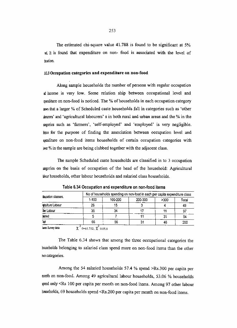
253
The estimated chi-square value 41.788 is found to be significant at 5%
Jei. It is found that expenditure on non- food is associated with the level of
mcation.
jj.3 Occupation categories and expenditure on non-food
Along sample households the number of persons with regular occupation
DI income is very low. Some relation ship between occupational level and
~diture on non-food is noticed. The % of households in each occupation category
OOWS that a larger % of Scheduled caste households fall in categories such as 'other
Wlourers' and 'agricultural labourers' s in both rural and urban areas and the % in the
;ategories such as 'farmers', 'self-employed' and 'employed' is very negligible.
Hence for the purpose of finding the association between occupation level and
apenditure on non-food items households of certain occupation categories with
Ilwer % in the sample are being clubbed together with the adjacent class.
The sample Scheduled caste households are classified in to 3 occupation
categories on the basis of occupation of the head of the household: Agricultural
labour households, other labour households and salaried class households.
Table 6.34 Occupation and expenditure on non-food items
ImIpation classes. No of households spending on non-food in each per capita expenditure class
1-100 100-200 200-300 >300 Total
~Iture Labour 26 15 3 4 49 "'rLabour 35 34 17 11 97 !laried 5 7 11 31 54 lolal 66 56 31 46 200 !ooR2: Survey data
l l X 0=61.752, X 0.05,6
The Table 6.34 shows that among the three occupational categories the
households belonging to salaried class spend more on non-food items than the other
two categories.
Among the 54 salaried households 57.4 % spend >Rs.300 per capita per
month on non-food. Among 49 agricultural labour households, 53.06 % households
spend only <Rs 100 per capita per month on non-food items. Among 97 other labour
households, 69 households spend <Rs.200 per capita per month on non-food items.

254
Of the 46 households who spend greater than Rs. 300 per capita per
month on non- food 31 belonged to salaried class, 11 belonged to other labour
lIouseholds and 5 belonged to Agriculture labour households
Of the 66 households who spend less than Rs.1 00 per capita per month on
non-food, only 5 belonged to salaried class 35 to other labour households and 26 to
agricultural labour households.
The estimated,l value (61.752) is found to be significant at 5 % levds. It
is found that expenditure on non-food is associated with the type of occupation.
6.9.3.4 Rural Urban Factor and expenditure on Non-food items
Table 6.35 gives the relationship between place of residence factor and
per capita expenditure on non-food. The Sample Scheduled caste households have
been classified in to two categories based on the place of residence namely, rural and
urban. The 200 sample households have been grouped into 4 per capita expenditure
classes on the basis of expenditure on non-food items
Scheduled caste households belonging to urban sector show tendency of
spending more on non-food item than rural Scheduled caste households.
Among the sample households in rural areas, 74% of households spent
<Rs.200 per capita per month on non-food items in rural while 15% households
spend >Rs. 300 per capita per month on non- food items.
Among 100 urban samples only 48% households spend <Rs.200 per
capita per month on non-food and 32% households spend >Rs 300 per capita per
month on non-food. Among the 66 Scheduled caste households, who spend below
Rs.lOO per capita per month on non-food, 73% belong to rural and only 27%
belonged to urban sector. Similarly among the 47 Scheduled caste households who
spend above Rs.300 per capita per month on non-food, 68% belonged to urban sector
and only 32% belonged to rural sector.

255
It is found that rural Scheduled caste consumers tend to spend less on
m-food than their counter parts in urban sample.
Table 6.35 Rural urban Factor and expenditure on Non-food items
Region No of households spending on non-food item each per capita expenditure class
1-100 100-200 200-300 >300 Total
Rural 48 26 11 15 100
Urban 18 30 20 32 100
Total 66 56 31 47 200
_ Survey data 2 2 X 0 =22.684. X 0.05,3 =7.815
The estimated X2 value (22.684) is found to be significant at 5% level for
j d.f. There is association between level of non-food expenditure and region of
IlSidence. Urban households spend more on non-food consumption.
Hence the third hypothesis is accepted that there is significant association
Oetween consumption expenditure and income, education, occupation and area of
residence.
6.10 Monthly Per capita Consumption Expenditure among Decile groups
Differences in consumption pattern of poorer and richer segment of
population (ranked by MPCE) in the sample area has been attempted by using in
appropriate deciles of the MPCE distnbution of class limits
Tables 6.36 and 6.37 give consumption of broad groups of food and non
food items per person for a period of 30 days for each decile group. It is observed that
regarding food consumption lowest 10 % of popUlation account for 4.75 % of the
total MPCE for the entire rural sample, while top 10% account for 13.32% that is 3
limes higher than the % for lowest decile group.
Among food items the highest expenditure of the top 10% is for Milk &
milk products. Other items are Fruits, Meat, fish & egg, Pulses, cooked food
purchased and Edible oil. While for the lowest decile group the highest % is for the
item Cereals. Other items are Salt, Spices, Sugar, and Edible oil.

256
It is found that regarding non-food consumption lowest 10% of
popUlation account for only 2.83% of the total MPCE for the entire rural sample
while top 10% account for 19.23 % i.e. About 6 times greater than % for the lowest
decile group. Among non-food items for the top decile group items attracting more
expenditures are Miscellaneous goods and services, Entertainment. Durable goods,
other miscellaneous goods and Travel.
Figure 6.4 Monthly Per capita Consumption Expenditure.among Decile groups
III
,. le
7t
t" tse
fa .. Ill. It
ID
0
• ............................. ........... a ......................... + .............. .
• • •
2 3 4 5 6 7 8
Decile group
•
9
-+- Ru ... 1 Food --RI ... " 101 food ..... Urbaa· Food ....... Urbaa • loa food
•
10 11
The figure shows that the households in the bottom decile groups for both
rural and urban sector spend greater % of total expenditure on food compared to top
decile group. For the top decile group % of expenditure on non-food is found very high.
For the lowest decile group the item attracting highest expenditure is Fuel
& light. All other non-food items constitute only very low % of expenditure
compared to higher decile group. It is found that the disparities among Scheduled
castes in the distribution of consumption expenditure is much higher in the rural
sector. Disparities in MPCE can be assumed to be the reflection of prevalence of wide
spread inequalities in the distribution of income, educational and occupation
differences among households in the sample area.

257
Table 6.36 Percentage of consumption of broad groups of food and non-food items per person for a period of 30 days for each declle group - Rural
terns Bottom 10% 10-20% ~30% ~% ~0-5O% 50-60% ~0-70% ~0-80% 80-90% ~op 10%
Cereals 7.68 9.07 9.39 10.46 8.31 10.60 11.68 11.72 14.47 6.63
PUlses 3.05 3.81 6.85 10.43 4.n 10.41 11.86 14.99 16.52 17.31
~ilk & milk products 1.54 5.40 3.16 8.03 3.95 10.05 18.39 16.21 7.95 25.32
dibleoil 4.98 4.94 8.06 8.69 5.92 14.43 10.34 11.12 15.33 16.19
Meat, fish & egg 3.45 4.13 6.19 7.29 6.96 10.63 10.92 16.57 16.42 17.44
Vegetables 3.83 4.60 7.01 6.04 4.02 9.02 12.27 21.43 17.28 14.50
ruits 3.17 5.00 8.13 9.17 7.33 10.45 13.88 10.98 11.07 20.81
~ugar 5.83 5.06 8.25 7.65 8.10 12.49 10.16 11.95 18.72 11.79
~verages 3.47 5.35 6.63 7.16 6.25 11.16 12.05 17.93 17.53 12.46
Salt 7.43 8.65 10.57 10.93 7.08 9.29 17.77 9.22 10.52 8.52
Spices 5.93 5.59 7.83 10.68 9.18 12.34 9.85 11.55 14.00 13.06
Cooked food purchased 0.15 0.99 1.49 5.64 6.06 5.87 3.63 23.06 36.31 16.81
ood total 4.75 5.83 7.14 8.66 6.99 10.27 10.99 14.81 17.25 13.32
Pan, tobacco & intoxicants 2.65 5.67 8.82 6.32 6.25 10.65 8.93 11.55 21.70 17.46
uel & light 7.93 7.56 9.07 9.60 7.63 9.49 9.83 10.82 14.29 13.77
Clothing 3.04 4.66 5.53 7.10 6.31 11.24 12.30 13.51 15.48 20.84
Footwear 2.74 3.12 4.60 6.59 4.00 10.78 18.39 15.09 16.53 18.16
ducation 3.56 4.95 9.71 3.07 4.94 3.18 15.15 20.70 16.50 18.25
~edical 2.35 3.13 4.05 4.79 5.40 10.08 10.52 11.11 38.13 10.45
ntertainment 0.00 3.94 2.75 5.00 4.15 3.28 13.42 17.03 22.83 27.60
Goods for personal care 4.22 3.47 6.51 8.21 6.04 8.53 14.63 14.64 17.09 16.67
Contribution 0.21 0.23 1.12 4.86 5.07 8.58 25.40 21.35 7,98 25.20
~ise. consumer goods 1.75 2.21 3.55 6.21 5.28 7.56 18.89 17.89 14.37 22.28
Ilravel 0.23 2.37 2.67 5.33 4.33 4.41 15.57 23.79 17.08 24.23
~ent 0.00 0.00 0.00 0.00 0.00 0.00 0.00 0.00 0.00 0.00
axes 0.00 0.61 0.00 0.00 0.00 24.15 34.66 28.98 ·0.00 11.59
Mise. goods and services 1.36 2.24 3.31 5.95 5.01 6.85 18.13 19.44 14.99 22.72
purable goods 0.02 0.16 0.15 4.12 2.17 7.14 13.37 13.90 32.66 26.31
~I non food total 2.83 4.10 5.79 6.26 5.53 8.87 12.75 14.34 20.30 19.23
~otal consumer expenditure 3.92 5.09 6.56 7.62 6.36 9.67 11.75 14.60 18.57 15.87
Source: Survey data
All
100
100
100
100
100
100
100
100
100
100
100
100
100
100
100
100
100
100
100
100
100
100
100
100
p.OC
100
100
100
100
100

258
Table 6.37. Percentage of consumption of broad groups of food and non-food items
per person for a period of 30 days for each decile group· Urban
Items Bottom 10-20% 20-30% 30-40% 10% 40-50% 50-60% 60-70% 70-80% 80-90% Top 10%
Cereals 2.41 6.31 3.86 7.90 8.37 7.94 8.98 14.22 14.86 25.15 Pulses 0.50 2.22 1.23 3.23 5.95 4.62 6.71 15.60 14.43 45.51 Milk & milk products 0.00 0.00 0.10 2.43 4.50 3.00 9.23 6.86 17.64 56.25 Edible 0 1.17 2.03 2.72 4.22 6.43 7.97 8.93 13.75 16.12 36.66 Meat, fish & egg 0.76 0.92 2.22 2.38 8.16 6.32 10.05 15.32 16.86 37.01 Vegetables 0.75 2.71 3.36 3.70 5.55 4.70 6.98 9.14 21.47 41.63
Fruilf 1.39 2.38 1.83 3.14 6.56 4.73 6.97 15.99 17.81 39.19
Sugar 1.48 5.19 3.91 5.19 9.17 7.91 7.42 15.95 14.97 '"'0 "" ~o.ov
Beverages 0.67 0.82 1.93 3.79 7.64 7.88 7.72 13.95 17.29 38.31
Salt 2.48 6.41 4.69 7.93 11.85 10.99 9.71 14.42 12.85 18.68
Spices 1.04 3.82 2.37 4.07 6.47 6.79 8.80 13.97 15.45 37.22
Cooked food purchased 0.00 0.58 3.53 5.40 9.00 11.88 3.68 17.57 15.78 32.59
Food total 1.23 3.12 2.77 4.87 7.41 6.99 8.12 13.90 16.40 35.20
Pan, tobacco & intoxicants 1.03 2.16 5.64 8.23 5.43 13.99 12.76 13.78 17.10 19.89
Fuel & light 2.58 5.53 3.43 7.18 9.99 10.78 8.58 15.14 13.83 22.96
Clothing 0.99 1.71 1.61 2.68 6.39 4.39 6.44 12.75 17.78 45.27
Footwear 0.49 1.87 1.22 2.62 5.67 4.56 6.69 13.02 15.42 48.44
Education 0.66 0.79 0.90 3.00 9.68 3.68 6.46 7.34 19.10 48.40
Medical 0.89 3.65 0.94 3.88 5.63 10.63 8.34 12.89 29.63 23.53
Entertainment 1.35 0.37 1.84 1.84 8.12 2.00 2.75 10.26 19.63 51.85
Goods for personal care 1.03 2.57 1.96 3.70 6.99 7.22 9.52 14.17 15.64 37.20
Contribution 0.00 1.62 0.44 0.65 6.23 1.22 1.99 3.74 11.36 72.75
Misc. consumer goods 0.65 1.88 1.32 2.20 6.84 4.05 5.51 9.38 14.45 53.71
Travel 0.99 0.71 0.61 1.47 5.85 5.18 2.77 4.75 11.58 66.09
Source: Survey data
All
100
100
100 100
100
100
100 , ,,,, .vv
100
100
100
100
100
100
100
100
100
100
100
100
100
100
100
100
We find that in the consumption of food the lowest declie group account
for 1.23% of the total MPCE while the highest decile group in the urban sector
accounted for 35.20% of total MPCE on food. The condition of the lowest decile is
found to be much worse in the urban sector than rural sector. The disparities between
Scheduled caste households in the distribution of total MPCE is found to be higher in
urban sample than rural sample.
The comparatively better position of rural Scheduled castes than urban
Scheduled castes belonging to lowest decile group may be considered to be the result
of the fact that consumption out of home grown stocks, through gift or loan
substitutes purchases in cash to a certain extent in rural sector. Other items attracting

259
more expenditure for lower decile group are Cereals, Salt, Sugar, and Edible oil. For
top decile group items with more expenditure are Milk & milk products, Vegetables,
Beverages, Fruits, and meat fish & egg. It is found that the top decile SC population
spend lavishly on these items. This is in tune with the general trend among Kerala
households in both urban and rural especially belonging to higher MPCE classes.
Among non-food items it is found that lowest 10% of the population
account for 1.04% to total MPCE on non-food bi urban sample households. While
-top 10% account for 43.48%. Lowest decile group being unable to spend even enough
for food do not find a place in the non-food expenditure at all. Of the total
expenditure on most of the non-food items, the top decile group constitutes a major
share. The important items are Miscellaneous goods and services, Entertainment,
Durable goods, Clothing and Footwear. The disparities in MPCE distribution is found
to be wider in urban than in rural sector among SC's.
Figures 6.5 and 6.6 gives Consumption of food and non-food items in
rural and urban group in bottom 10-% group. Figure 6.7 and 6.8 gives Consumption
of food and non-food items in rural and urban group in top 10-% group. There is
widespread differences observed the distribution of total expenditure between food
and non-food items between the bottom and top decile groups. Hence the second
hypothesis is accepted that there is significant difference in the average consumption
expenditure of different decile groups.
Figure 6.5 MPCE on food and non-food items in rural for bottom Decile group
Rural
Source: Survey data
OFood
oNon food

260
Figure 6.6 MPCE on food and non-food items in urban for bottom Decile group
Urban
50% .Food
oNon food
Source: Survey data
Figure 6.7 MPCE on food and non-food items in rural for top Decile group
Rural
48% mJFood
oNon food
Source: Survey data
Figure 6.8 MPCE on food and non-food items in urban for top Decile group
I Urban I
Source: Survey data
El Food
ONonfood

261
6.11 Sources of consumption
As per the findings on the living standards of Scheduled castes by the
commission in 1982, the Scheduled castes had very low levels of consumption. Their
food items were, the little quantity of unhusked paddy they got as cooli; roots and
Fruits they collect from fields, fish they caught from paddy fields, and the carcass of
animals. The innutrition food, filthy habits, wretched conditions of life and ignorance
made their life miserable and somewhat similar to that of animals. In. the forest areas -they were collecting honey, forest produces and hunting. They hunted wild animals
for food.
These conditions of the Scheduled castes have undergone drastic changes.
The following table reveals the different sources of household consumption of
Scheduled castes at present for the sample areas.
Total expenditure includes consumption out of purchases, home grown
stock and gift or loan and free collection. The higher % of expenditure on certain
items such as Milk & milk products, Edible oil, Vegetables, meat egg, fish, Fruits,
and Spices is found to be due to the increased consumption out of home grown stock.
Table 6.38 gives different sources of total consumption expenditure for
sample rural and urban Households. Table shows that consumption out of cash
~urchase constitutes the major source of total consumption expenditure both in rural
and urban areas for all items.

Ta
ble
. 6
.38
Pe
rce
nta
ge
Of co
nsu
mp
tio
n o
ut o
f ca
sh
pu
rch
ase
, h
om
eg
row
n a
nd
gif
t lo
an
In
to
tal co
nsu
mp
tio
n e
xp
en
dit
ure
fo
r
rura
l a
nd
urb
an
sa
mp
les
for
dif
fere
nt i
tem
s.
Rice
& ot
her c
erea
ls Ve
geta
bles
M
eat f
ish e
gg
Oil
and
fats
M
ilk a
nd m
ilk p
rodu
cts
Frui
ts a
nd n
uts
Con
dim
ents
and
spi
ces
Fuel
and
ligh
t
Rura
l Ur
ban
Rur
al
Urb
an
Rura
l U
rban
R
ural
U
rban
R
ural
U
rban
R
ural
U
rban
R
ural
U
rban
R
ural
Ur
ban --
Cash
Pur
chas
e 91
.4
99.3
81
.2
96.6
95
.0
96.8
94
.4
100.
0 80
.6
92.9
42
.6
59.1
93
.4
96.2
46
.7
58.3
Hom
e gr
own
5.3
0.1
18.6
3.
0 4.
8 2.
8 5.
6 0.
0 19
.4
7.1
49.2
22
.6
5.2
0.1
13.9
3.
6
Gift
loan
, fre
e co
llect
ion.
3.
3 0.
6 0.
2 0.
4 0.
3 0.
4 0.
0 0.
0 0.
0 0.
0 8.
2 18
.3
1.4
3.7
39.4
38
.2
Tota
l 10
0.0
100.
0 10
0.0
100.
0 10
0.0
100.
0 10
0.0
100.
0 10
0.0
100.
0 10
0.0
100.
0 10
0.0
100.
0 10
0.0
100.
0
Sour
ce: S
urve
y Da
ta
N
C\
N

263
It is found that consumption out of homegrown stock constitutes a good
e of total consumption among rural sample for many items of .consumption.
IOrtion of consumption out of homegrown stock is highest for the items Fruits &
: in both rural (49.2%) and urban (22.6%) sectors. People in Kerala are known for
r high consumption of coconut kernel and oil. According to household
sumption surveys, the per capita average intake of c(,~onut products in terms of oil
ivalent was 10.023 kg in 198518•
Other items reporting higher proportion of home grown stock in total
lSumption in rural sector are Milk & milk products (19.4%) and Vegetables
1.6%). Oil & fats, Cereals, Spices, meat, fish, & egg also show considerable
round 5%) proportion of home grown consumption in rural areas. In urban sector
is is a negligible phenomena for almost all food items except milk, Vegetables, and
[cat, fish & egg.
Proportion of consumption out of gift, loan and free collection constitutes
~gible % in both rural and urban sectors regarding almost all items of
llSumption. This indicates that there is significant change in the source of
ISehold consumption of Scheduled castes from the past periods. They are
~ding on their cash purchases or their own home grown products for
~ption and no much dependence is on the gifts or loans or free food items
lected or received from elsewhere in their total consumption.
! Per capita Consumption of Individual Items - food
Per capita expenditure estimates for different items of consumption
uding food, tobacco& fuel, Clothing and Footwear, Education and Medical
:use, and other miscellaneous items are presented based on sample data from rural
wan areas.
This section gives an analysis of the per capita consumption expenditure
IlD.ple rural and urban households on individual items. Sample households have
categorized in to various monthly per capita expenditure classes in Table 6.39.
of rural households and 84% of urban population come under the broad per

264
capita monthly expenditure class of Rs.1-800 and the remaining 6% in rural and 16%
in urban sectors among the sample population selected belonged to >Rs.800.
Table. 6.39 Distribution of sample households by mon IY per cap. consumpl.on eXI len • ure ful .~ f dl
Monthly per capita Rural Urban
consumption exPenditure No. of House % No. of % holds households
1·200 28 28 13 13
200-400 36 36 34 34
~600 20 20 20 20
600-800 10 10 17 17
>800 6 6 16 16 Source: Survey data
The per capita expenditure data collected under individual items of
consumption however cannot be accurate as there are chances of unaccounted
expenses and recall lapses
As per the table on average MPCE given earlier, average MPCE for the
rural sector was found to be Rs.372.57 and for the urban sector Rs.526.20. Average
MPCE on food items for rural sector was found to be Rs.21 1.90 (56.88%) and for the
urban sector Rs.239.23 (45.48%). For the non-food items average MPCE for rural
sector was Rs.160.67 (43.12%) and for urban sector Rs.286.97 (54.54%).
6.12.1 Consumption of Cereals
Of the 200 sample households the expenditure data on Cereals of all
households were available. The Table 6.40 shows that the number of households,
which spent between Rs.50-60 per person monthly, was highest in the sample in both
rural as well as urban. Nearly 19% of the households fell under this expenditure class
in the rural area and 21 % in the urban.

265
Table 6. 40 Monthly per capita expenditure on Cereals by households
Per capita Rural Urban
Expenditure class No. households % Cu. No. of households % Cu. Frequency Frequency
Below-30 2 2 2 3 3 3
30-40 9 9 11 9 9 12
40-50 13 13 24 14 14 26
50-60 19 19 43 21 21 47
60-70 12 12 55 17 17 64
70-85 18 18 73 13 13 77
85-100 13 13 86 6 6 83
Above-100 14 14 100 17 17 100
Total 100 100 100 100
Source: Survey data
There were 11 % of families in rural sample whose per capita expenditure
per month on Cereals was below Rs. 40 and the corresponding % in urban sample
was 12. Families, which consumed Cereals worth less than Rs.1.66 per person a day
(Less than Rs.50 per head per month) was more than 20% in rural and nearly 26%in
urban areas. The % of families whose per capita daily expenditure on Cereals
exceeded Rs.3.33 was 14% in the rural area while the % in urban was 17%. Mean
cereal expenditure for the rural sample was RS.71.92 and urban sample was Rs. 68.52.
[As per Table 6.20]
6.12.2 Consumption of Pulses
Pulses do not form major consumption item for all the sample families.
Table 6.41 shows that about 30% of the households in rural did not expend any
amount on Pulses and 26% in urban. In addition 77% of those who consumed Pulses
in rural spent only less than Rs.I0 per head a month and likewise more than 60%in
urban. If those who expended less than Rs.20 per person are included, the % of those
who spent nominally on this item in rural will go up adding another 18% in rural and
26% in urban.

266
Table 6.41 Monthly per capita expenditure on Pulses by households
Perca~ita Rural Urban
Expenditure class No.of % Cu. No.of households % Cu. households freQuency frequency
- 1-10 54 n,14 n,14 45 60.81 60.81
10-20 13 18.57 95.71 19 25.68 86.49
20-30 2 2.86 98.57 , 7 9.46 95.95
30& Above 1 1.43 100 3 4.05 100
Total 70 100 74 100
Source: survey data
The majority of the house holds came under the expenditure class of
below Rs 10. During the survey it is noticed that generally poor families do not
consume Pulses though they expend on cosmetics and toiletries. Extreme cases of
Pulses consumption (Rs.30& above) were found among only 1 % of the sample rural
household and 4% among urban households
6.12.3 Consumption of Milk & milk products
The Table 6.42 shows that 64 sample Scheduled caste households are
missing from Milk & milk products consumption in rural and 57 in urban. They could
not afford to spend on this item as they belonged to the lower il1come category; even
though it is a nutritious item. Among those who spend 70% belonged to the per capita
expenditure classes of below Rs. 30 in rural sample and 40 % in urban sample. There
were only 2 households whose per capita consumption was wroth more than Rs.60 a
month in rural area and 7 households in urban.
It was noticed that many of them who belong to higher expenditure
classes were not particular about spending on milk though they allocate pretty good
amount to the consumption of meat, egg and fish. This indicates the particular food
habits of Scheduled castes in the study area and their preference to non-vegetarian
food.

267
T bl 642 M hi d't a e . ont Iy per capita expen I ure on M'lk& 'Ik d b h I ml pro ucts ,y ouseholds
Per capita Expenditure Rural Urban
class No of % Cu. No. of % Cu. households Frequency households Frequency
1-10 6 16.67 16.67 3 6.98 6.98 10-20 8 22.22 38.89 3 6.98 13.96 20-30 11 30.56 69.45 11 25.58 39.54 30-40 4 11.11 80.56 7 16.28 55.82 40-50 3 8.33 88.89 7 16.28 72.10 50-60 2 5.56 94.45 5 11.63 83.73
Above 60 2 5.56 100 7 16.28 100 Total 36 100.00 43 100
SoIIca: SuMy data
6.12.4 Consumption of Edible oil
Among the rural sample Scheduled caste households all households
reported expenditure on Edible oil.50%of the families belonged to the per capita
monthly expenditure class of below Rs.I0 in rural area and 41 %in urban area. The
households, which expended more than Rs.30 per head, formed 6% of the sample in
rural and 12% in urban sample.
T bl 643 M thl 't a e . on Iy per capl a expen d't I ure on Ed'bl 'I b h I eOI ,y h Id ouse 0 S
Per capita Expenditure Rural Urban
class No.of % Cu. No.of % Cu. households Frequency households Frequency
1-10 50 50.00 50 41 41.41 41.41 10-20 36 36.00 86 27 27.27 68.68 20-30 8 8.00 64 19 19.19 87.87 30-40 4 4.00 98 7 7.07 94.94
Above 40 2 2.00 100 5 5.05 100 Total 100 100.00 99 100
Source: Survey data
. It was noticed that both rural and urban consumers are not inclined to the
consumption of sophisticated oil brands. Most of the consumers are not using modem
types of oil.
6.12.5 Consumption of Sugar
All rural and urban sample households had spent on Sugar consumption.
The households clustered in the expenditure classes of below Rs.20.constituted 97%

268
in rural and 90%in urban. Sugar as a food item, cannot be consumed at a higher level
due to health reasons. Even the middle-income families had not spent much on this
item, unlike any non-food items. The level of Sugar consumption would not go up
beyond a certain level unlike in the case of non-food, non -essential commodities.
Table 6,44 Monthly per caDita expenditure on Sugar by households
Per capita Expenditure Rural Urban
class No. of % Cu. No. of % Cu. households frequency households Frequency
1-10 81 81.00 81 61 61.00 61
10-20 16 16.00 97 29 29.00 90
Above 20 2 3.00 100 10 10.00 100
Total 100 100.00 100 100 Source: Survey data
6,12.6 Consumption of Meat, fish & egg.
As revealed in the secondary data analysis the Scheduled castes of Kerala
prefer non-vegetarian food. It is found that the consumption of Meat, fish & egg
constitutes one of the prominent items in the consumption basket of Scheduled castes
The primary data showed that for a considerable % sample population, it is an
inevitable item of consumption. They are able to spend only a relatively small amount
on this item.
T bl 645 M thl 't a e. , on IY per capl a expen d't I ure on M t f' h & ea I IS b h h Id egg )Y ouse 0 S
Per capita Expenditure Rural Urban
class No.of % Cu. No.of % Cu. households Frequency households Frequency
1-10 26 27.96 27.96 27 27.84 27.84 10-20 29 31.18 59.14 17 17.53 45.37 20-30 13 13.98 73.12 18 18.56 63.93 30-40 9 9.68 82.80 12 12.37 76.30 40-50 4 4.30 87.10 4 4.12 80.42 50-60 4 4.30 91.40 6 6.19 86.61 60-70 3 3.23 94.63 3 3.09 89.70 70-85 2 2.15 96.78 4 4.12 93.82 85-100 1 1.08 97.86 4 4.12 97.94
Above 100 2 2.15 100 2 2.06 100 Total 93 100.00 97 100
Souroe: SuMy data

269
Table 6.45 show that 28 % of both the rural and urban sample households
spend only below Rs.I0 on the item. While in the rural sector 31.18% of household3
spend Rs. 10-20 on the item in the urban the % was 17.53. Thus 59% in rural and
45.37% in urban spend below Rs 20 on the item. 13% of households in rural and 20% in
urban had an average per capita expenditure of more than Rs. 50 on the item. Thus the
upper expenditure classes spend more on the item among sample Scheduled caste
households
6.12.7 Consumption of Vegetables
In the rural sector 7 households are missing from the vegetable
consumption and 9 in urban. Table 6.46 shows that among those who spend on the
item, 72% in rural and 71 % in urban spend below Rs.20 per capita per month on the
item. In the rural sector only 5.39% and in urban 6.60 % of households spend more
than Rs. 50 on Vegetables. Vegetable was one of the items for which consumption
out of homegrown stock was reported. It was found that consumption of Vegetables
was not as common as meat, egg & fish among the sample households.
Table.6.46 Monthly per capita consumption expenditure on V t bl b h h Id ege a es )y ouse 0 S
Per capita Expenditure Rural Urban
class No.of % Cu. No.of % Cu. households Frequency households Frequency
1-10 40 43.01 43.01 35 38.46 38.46 10-20 27 29.03 72.04 29 31.87 70.33 20-30 6 6.45 78.49 9 9.89 80.22 30-40 10 10.75 89.24 7 7.69 87.91 40-50 5 5.38 94.62 5 5.49 93.40
Above 50 5 5.39 100 6 6.60 100 Total 93 100.00 91 100
Source: Survey data
6.12.8 Consumption of Fruits & nuts
As per Table 6.47 it was found that 8% of the sample households did not
consume either Fruits or nuts in rural and 4%. In rural sector 49.2 % of the
consumption of Fruits & nuts was out of homegrown stock and in the urban sector
consumption out of home grown stock constituted 22.6 % of the total consumption of
the item. This has been presented in table 6.38.1t is apparent that consumption of this
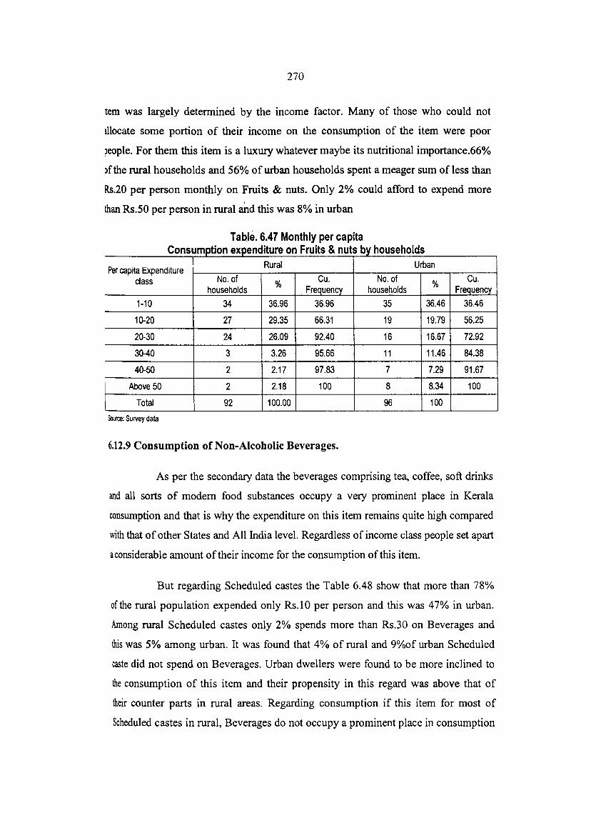
270
tern was largely detennined by the income factor. Many of those who could not
lllocate some portion of their income on the consumption of the item were poor
~eople. For them this item is a luxury whatever maybe its nutritional importance.66%
i)f the rural households and 56% of urban households spent a meager sum of less than
Rs.20 per person monthly on Fruits & nuts. Only 2% could afford to expend more
than Rs.50 per person in rural and this was 8% in urban
Table. 6.47 Monthly per capita c onsumptlon expen I ure on rUI s nu s ,y ouse 0 S d't F't & t b h h Id
Per capita Expenditure ! Rural Urban
class No. of % Cu. No. of % Cu. households FreQuency households FreQuency
1-10 34 36.96 36.96 35 36.46 36.46
10-20 27 29.35 66.31 19 19.79 56.25
20-30 24 26.09 92.40 16 16.67 72.92
30-40 3 3.26 95.66 11 11.46 84.38
40-50 2 2.17 97.83 7 7.29 91.67
f;;bove 50 2 2.18 100 8 8.34 100
Total 92 100.00 96 100
Source: Survey data
6.12.9 Consumption of Non-Alcoholic Beverages.
As per the secondary data the beverages comprising tea, coffee, soft drinks
and all sorts of modem food substances occupy a very prominent place in Kerala
consumption and that is why the expenditure on this item remains quite high compared
with that of other States and All India level. Regardless of income class people set apart
aconsiderable amount oftheir income for the consumption of this item.
But regarding Scheduled castes the Table 6.48 show that more than 78%
of the rural population expended only Rs.I0 per person and this was 47% in urban.
Among rural Scheduled castes only 2% spends more than Rs.30 on Beverages and
this was 5% among urban. It was found that 4% of rural and 9%of urban Scheduled
caste did not spend on Beverages. Urban dwellers were found to be more inclined to
the consumption of this item and their propensity in this regard was above that of
their counter parts in rural areas. Regarding consumption if this item for most of
Scheduled castes in rural, Beverages do not occupy a prominent place in consumption

... ..." L. I 1
basket. But the higher MPCE classes of rural and urban samples show preference to
this item.
Table 6.48 Monthly per capita expenditure on Beverages by households
I Per capita Expenditure Rural Urban
I class No. of Cu. No. of Cu. households
% Frequency households
% Frequency
1·10 75 78.13 78.13 43 47.25 47.25
10-20 16 16.67 94.80 36 39.56 86.81
20·30 3 3.13 97.93 7 7.69 94.50
Above 30 2 2.08 100 5 5.49 100
I Total 96 100.00 91 100
Source: Survey data
6.12.10 Consumption of Spices
As per Table 6.49 out of 99 families 83% of the households fell in the
expenditure class of below Rs.20 per head in rural and out of a sample of 100 families
78% fell ir. the expenditure class of below Rs 20 per head in urban. Like Cereals,
Spices also constitute an ingredient in Scheduled castes diet. It is an inevitable item in
the food basket of rural and urban Scheduled castes. 5.05%of Scheduled castes in
rural belonged to the expenditure class of above Rs 30 and the same was 6% in case
of urban sector.
Table 6.49 Monthly per capita expenditure on Spices by households
i Per capita Expeflditure Rural Urban
: class No. of I % Cu. No. of % Cu.
i I
l
households Frequency households Frequency
1·10 40 40.40 40.40 41 41.00 41
10·20 42 42.42 82.82 37 37.00 78 .'
20·30 12 12.12 94.94 16 16.00 94
Above 30 5 5.05 100 6 6.00 100
Total 99 100.00 100 100
Source: Survey data
6.12.11 Consumption of Salt
As per Table 6.50 out of the 100 rural families, 99% of households fell in
the expenditure class of below Rs.20 per head and all the 100 urban families fell -.-
under this category.

272
Table 6, 50 Monthly per capita expenditure on Salt by households
Per capita Expenditure Rural Urban
class No. of % Cu. No. of % Cu. households FreQuency hOuseholds Frequency
1-10 99 99.00 99 100 100.00 100
10-20 1 1.00 100 0 0.00 0
Total 100 100.00 100 100
Source: Survey data
Extreme levels of consumption are not found here. This IS perhaps
because there is a limit for the quantity for salt that one could consume.
6,12.12 Expenditure on cooked food purchased
Table 6.51 shows MPCE on cooked food purchased for the sample households.
T bl 651 M thl 't t' a e , on Iy per capl a consumpllon expen d't k d f d h d I ure on coo e 00 purc ase
I Per ca~ta Expenditure Rural Urban
class No. of % Cu. No. of % Cu. households Frequency households Frequency
1-50 21 53.84 53.84 32 66.66 66.66
50-100 10 25.64 79.48 14 29.16 95.82
Greater than 100 8 20.51 100 2 4.16 100
Total 39 100.00 48 100
Source: Survey data
I
It was found that about 60% of the total rural households did not spend on
cooked food purchased from outside their homes and more than half of those who
spend spend less than Rs. 50 per capita per month on the item. There are 20% of
households who spend more than Rs. 100 on the item in the rural sector. It was found
that most of the Scheduled castes in the sample area being agricultural laboures or
other labourers they are far off in their work place and are unable to take food from
their own houses, Not only that some of them consider it as convenient. In the urban
sector about 67% of households spend less than Rs 50 per capita per month on the
item. Among the urban households 62% reported consumption of the item urban
households showed more preference towards spending on the item especially those in

273
the higher MPCE. classes. This might be intune with the emerging conspicuous
consumption pattern among the higher income groups in Kerala as per NSSO data.
6.13 Per capita consumption of individual items: Non-food
Monthly per capita consumption expenditure on non-food items has also
been analysed to understand the difference between expenditures on food and non
food items.
6.13.1 Consumption of Pan, tobacco & intoxicants
Pan, tobacco & intoxicants form a major consumption item for almost all
the sample households. Table 6.52 shows that out of the total 200 households 184
households spent on the item. Consumption of Pan, tobacco & intoxicants is at very
high level among Scheduled castes as per the sample data. Expenditure incurred on
the items indicates that a considerable % of the popUlation consume extravagantly. In
the rural sector number of households who spend on the item is higher in the lower
expenditure classes as compared to urban. 57 % of those who spend on the item in
rural areas and 37% in urban areas have an average monthly expenditure below Rs.
30. 22% of those households in the rural sector have an average per capita
expenditure of Rs.30-60, while in the urban sector it is 36%. Similarly 10 % of rural
households have an average per capita expenditure of Rs.60-100 and the
corresponding % in urban sector was 15%. Among those who spend on the item in
rural 10% spend Rs.100-250 per capita per month on the item and for urban sample
this was 13%. It is found that moving to higher expenditure classes in the rural sector
the sample Scheduled caste households spend extravagantly on Pan, tobacco &
intoxicants. Also in rural sector even among lower expenditure classes the
expenditure on the item is found much higher. The low per capita income position of
the households along with higher expenditure on pan, tobacco, drugs & intoxicants
adversely affects their consumption standard. It is observed that those households
having larger expenditure on the item especially in the lowest expenditure classes
have not even the basic consumption requirements. This is true in case of both rural
and urban households in the sample areas and this is one of the most important
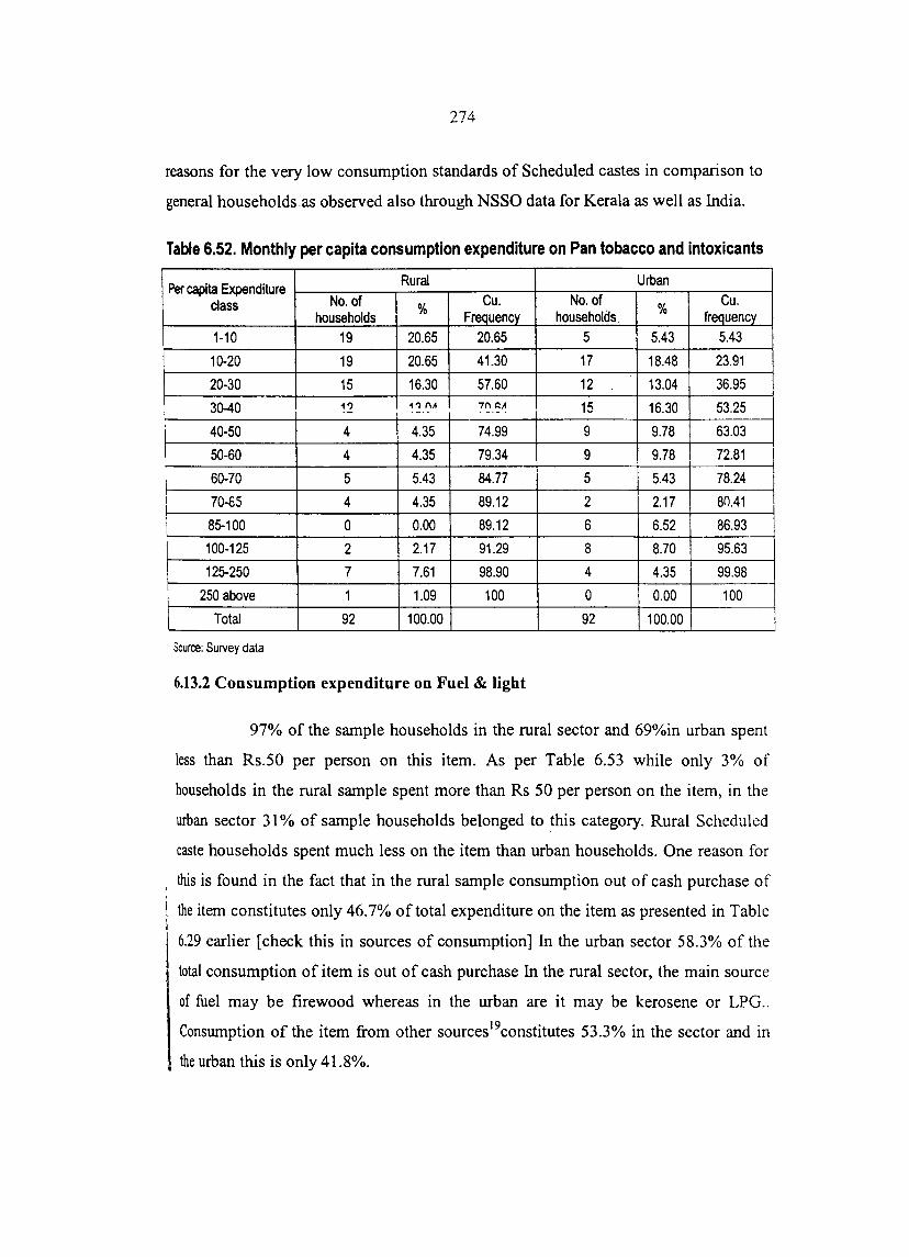
274
reasons for the very low consumption standards of Scheduled castes in comparison to
general households.as observed also through NSSO data for Kerala as well as India.
Table 6.52. Monthly per capita consumption expenditure on Pan tobacco and intoxicants
Per capita Expenditure Rural Urban
class No. of % Cu. No. of % Cu. households Frequency householas. frequency
1-10 19 20.65 20.65 5 5.43 5.43
10-20 19 20.65 41.30 17 18.48 23.91
20-30 15 16.30 57.60 12 13.04 36.95
30-40 1? 1~ nA 7n t::A 15 16.30 53.25 . -'- . . -'- .
40-50 4 4.35 74.99 9 9.78 63.03
SO-60 4 4.35 79.34 9 9.78 72.81
60-70 5 5.43 84.77 5 5.43 78.24
70-65 4 4.35 89.12 2 2.17 80.41
85-100 0 0.00 89.12 6 6.52 86.93
100-125 2 2.17 91.29 8 8.70 95.63
125-250 7 7.61 98.90 4 4.35 99.98
250 above 1 1.09 100 0 0.00 100
Total 92 100.00 92 100.00
Source: Survey data
6.13.2 Consumption expenditure on Fuel & light
97% of the sample households in the rural sector and 69%in urban spent
less than Rs.50 per person on this item. As per Table 6.53 while only 3% of
households in the rural sample spent more than Rs 50 per person on the item, in the
urban sector 31 % of sample households belonged to this category. Rural Scheduled
caste households spent much less on the item than urban households. One reason for
this is found in the fact that in the rural sample consumption out of cash purchase of
the item constitutes only 46.7% of total expenditure on the item as presented in Table
6.29 earlier [check this in sources of consumption] In the urban sector 58.3% of the
total consumption of item is out of cash purchase In the rural sector, the main source
of fuel may be firewood whereas in the urban are it may be kerosene or LPG ..
Consumption of the item from other sources19constitutes 53.3% in the sector and in
the urban this is only 41.8%.

275
Table 6,53 Monthly per capita expenditure on Fuel & lights by households . I
Per capita Expenditure i Rural I Urban
class No. of % Cu. ··No. of % Cu.
households Frequency households FreQuency 1-10 8 8.00 8 0 0.00 0
10-20 52 52.00 60 8 8.00 8
20-30 25 25.00 85 19 19.00 27
30-40 10 10.00 95 18 18.00 45 40-50 2 2.00 97 24 24.00 69
50-60 1 1.00 98 12 12.00 81
60&above 2 2.00 100 19 19.00 100
Total 100 100 100 100 _. -_._- -- - --
Source: Survey data.
6,13.3 Consumption expenditure on clothing
Table 6.S4 indicates that among the rural and urban sample households,
higher expenditure classes, expenditure on Clothing increases rapidly. In the rural
sector per capita expenditure on Clothing for the lowest 7% of households were
below Rs.SO and the corresponding in urban was 6%. 21 % of households rural and
10% in urban spend Rs. SO-lOO per capita per month on the item. 72% of households
in rural and 83% in urban spend Rs. 100-2S0 per capita per month on Clothing.
Secondary data analysis has shown that expenditure on Clothing is very
high among households in Kerala. As per sample data it is found that Scheduled caste
households in the lower MPCE classes spend very less on the item in both sectors and
those in higher MPCE classes follow !he general consumption trend observed in
Kerala for the item.
T bl 654 M thl 't a e , on IY per capl a expen d't I ure on Cl th' b h 0 mg )y h Id ouse 0 S
Per capita Expenditure Rural Urban.
class No. of % Cu. No. of % Cu.
households Frequency households Frequency 20-30 1 1.00 1.00 1 1.03 1.03 30-40 3 3.00 4.00 1 1.03 2.06 40-50 3 3.00 7.00 4 4.12 6.18 50-60 3 3.00 10.00 1 1.03 7.21 60-70 2 2.00 12.00 1 1.03 8.24 70-85 10 10.00 22.00 4 4.12 t2.36 85-100 6 6.00 28.00 4 4.12 16.48 100-250 72 72.00 100.00 81 83.5 99.98
Total 100 100 97 99.98
Source: Survey data.

276
6.13.4 Consumption expenditure on Footwear
The survey has revealed that nearly 36% of the households are not
spending any amount in their MPCE on the item. As per Table 6.55 of the 88
households who spent on the item in rural sample 65% spend on Footwear to the tune
of Rs.I-30 per head monthly. In the urban sector the corresponding % was 57%. In
the rural sample 20.45% spend on Footwear to the tune of Rs.30-70. In the urban
sector th~ corresponding % was 30.26. 14.78% of households in rural and 13.16% of
households in urban spend above Rs.70 per capita per month on Footwear.
The NSSO data showed that expenditure on this item by Scheduled castes
has gone up in recent years. During 1983 the average expenditure on the item for
Scheduled castes in rural sector in Kerala was Rs.0.39 that is 0.37 % of the total
MPCE. By 1987- 88 this has increased to Rs.0.83 ie. 0.50 % of total MPCE. In the
urban sector the corresponding change was from Rs. 0.54 ie.O.4% in 1983 to Rs.l.56
i.e. 0.85 % in 1987-88.
!
,
But in the all-India level the proportion of the total expenditure on this
item for Scheduled castes in rural sector has grown from Rs.0.79 ie. 0.83% of MPCE
in 1983 to Rs.1.18 ie 0.88% of MPCE in 1987-88 and to Rs.1. 73 ie 0.72% in 1993-
94.
T bl 655 M thl 't a e . on IIY per capl a expen d't I ure on F tw b h h Id 00 ear oy ouse 0 s Rural Urban
Per capita Expenditure class Number of %of Cum. F Number of % of households Cum. f
households households households
1-10 21 23.86 23.86 12 15.79 15.79
10-20 20 22.73 46.59 18 23.68 39.47
20-30 16 18.18 64.77 13 17.11 56.58 I
30-40 7 7.95 72.72 9 11.84 68.42
40-50 6 6.82 79.54 6 7.89 76.31
50-60 2 2.27 81.81 5 6.58 82.89
60-70 3 3.41 85.22 3 3.95 86.84
70&above 13 14.78 100.00 10 13.16 100.00
Total 88 100 76 100
Source: Survey data

I
I
277
6.13.5 Consumption expenditure on Education
Of the 200 households only 118 households reported to spend on
Education. That is 60% in rural and 58% in urban... Table 6.56 show per capita
expenditure on Education.
T bl 656 M thl a e . on Iy per capl a expen d't I ure on Ed t' b h uca Ion )y h Id ouse 0 S Rural Urban
Per capita Expenditure Number of %of Numberof ' %of Cu.
class Cum.F households households households households Frequency
10-20 4 6.67 6.67 2 3.45 3.45
20-30 1 1.67 8.34 2 3.45 6.90
30-40 4 6.67 15.01 2 3.45 10.35
40-50 4 6.67 21.68 4 6.90 17.25
50-60 5 8.33 30.01 0 0.00 17.25
60-70 5 8.33 38.34 1 1.72 18.97
70-85 6 10.00 48.34 2 3.45 22.42
85-100 8 13.33 61.67 4 6.90 29.32
100-250 23 38.34 100.01 41 70.68 100.00
Total 60 100 58 100
Source: Survey data
Since Scheduled castes receive the various types of financial assistance
for Education from government per capita expenditure estimates on the item
presented here may not be the actual picture. As per NSSO data the average MPCE
on Education among Scheduled castes has gone up in recent years. Of the households
reporting expenditure in the rural sector, 37% spend on the item between RsIO-IOO
per head per month.
In the urban sector 29.32% of households reporting expenditure, spent
between Rs.IO-IOO per head per month. In the urban sample 70.58% households
I spend between Rs 100-250 per head per month this and their % is much higher than
I, that of rural sample. Hence we find that urban Scheduled castes households in the
higher MPCE classes spent much more on the item per person compared to rural I : Scheduled caste households.
I

278
6.13.6 Consumption expenditure on Medical services
Medical expenditure is a very important item among . non-food
expenditure of Scheduled caste households. Expenditure on medicines and Medical
services of different households is detennined by a number of factors and hence
expenditure data on the item have been collected for last 30 days and also for
previous 365 days. In Table 6.57 average monthly per capita expenditure data is
presented. Nearly 17% of the households in rural are not spending any amounts on
Medical. In the rural sector, nearly 46% of the· Scheduled caste households, who
spend, spend below Rs 50 per person per month and in urban sector nearly 16%.
Among households belonging to the top expenditure class in the urban sector 84.53%
spend above Rs. 50 per capita per month as Medical expenditure and the
corresponding % for rural is 54.23%. Medical expenditure is found to be noticeably
higher per head in the upper MPCE class of urban sample than rural.
T bl 657 M thl 't a e , on Iy per capl a expen d't I ure on M d' Ib h e Ica ,y h Id ouse 0 S Rural Urban
Per capita Cu. Expenditure class Number of %of Cum.F Number of %of
households households households households Frequency
1·10 1 1.20 1.20 0 0.00 0.00
10-20 5 6.02 7.22 1 1.19 1.19
20·30 8 9.64 16.86 3 3.57 4.76
30-40 17 20.48 37.34 2 2.38 7.14
40-50 7 8.43 45.77 7 8.33 15.47
50&above 45 54.23 100.00 71 84.53 100.00
Total 83 100 84 100
Source: SUNey data.
6.13.7 Consumption expenditure on Entertainment
Table 6.58 shows that of the 200 households only 77 households spend on
entertainments. Among Scheduled caste households expenditure on the item is found
to be negligible in rural as well as urban sectors. About 85% of households who spent
on the item in the rural sector spent between Rs.I-20 per month. Scheduled caste
households in sample area are having much lower per capita expenditure on the item

279
and may be due to their lower income levels. Even in the urban sector about 84% of
households had the same expenditure pattern on the item. It is found that even for the .
upper MPCE classes of urban sector expenditure on Entertainment does not constitute
a major item among non-food items
Table 6.58. Monthly per capita expenditure on Entertainment by households
Per capita Rural Urban
Expenditure class Number of %of Cum.F Number of %of Cum.F households households households households
1·10 22 55.00 55.00 21 56.76 56.76
10-20 12 30.00 85.00 10 27.03 83.79
20-30 4 10.00 95.00 1 2.70 86.49
30-40 1 2.50 97.50 2 5.41 91.90
40·50 1 2.50 100.00 1 2.70 94.60
50&above 0 0.00 100.00 2 5.40 100.00
Total 40 100 37 100
Source: Survey data
It shows that the influence of place of residence is much less in the
determination of expenditure on recreation and Entertainment among Scheduled caste
households.
6.13.8 Consumption of Goods for personal care, toilet articles and sundry articles.
Table 6.59 shows that 85% in rural and 84% of households in urban spend
less thanRs.20. 97% of sample rural households and 94% of urban sample households
spend below Rs.50 per person on the items. Households belonging higher MPCE
classes spending more than Rs. 50 per person constitute only 4% in the urban sector
and 2% in the rural.
It is found that Scheduled caste popUlation of the sample area do not show
preference to spending more on cosmetics and other personal commodities and
whatever expenditure on the item is recorded is on account of expenditure on toilet
articles on which most of households recorded larger expenditures. Here rural urban
differences are not pronounced as in the case of certain other commodities.

i
280
T bl 659 M hi a e , , ont Iy per capita expenditure on G d f b h 00 s or persona care ,y h Id ouse 0 s Rural Urban
Per capita Expenditure class Number of %of Cum.F Number of %of Cu.
households households households households Frequency
1-10 56 57.14 57.14 36 36.36 36.36
10-20 31 31.64 88.78 25 25.25 61.61
20-30 7 7.14 95.92 29 29.29 90.90 (
30-40 1 1.02 96.94 3 3.03 93.93
40-50 1 1.02 97.96 2 2.03 95.96
50&above 2 2.04 100.00 4 4.04 100.00
Total 98 100 qq 100
Source: Survey data
6.13.9 Consumption Expenditure on Travel and conveyance
Besides Travel expenditure needs of households differ based upon the
nature of jobs, place of residence etc. Table 6.60 shows monthly per capita
expenditure on Travel by households.
a e on IY per capl a expen T bl 660 M thl 't d't I ure on T rave Ib h ,y h Id ouse 0 s
Per capita Rural Urban
Expenditure class Number of %of Cum.F Number of %of Cu. households households households households Frequency
1-10 3 4.76 4.76 2 3.28 3.28
10-20 3 4.76 9.52 4 6.56 9.84
20-30 4 6.35 15.87 3 4.92 14.76
30-40 3 4.76 20.63 4 6.56 21.32
40-50 7 11.11 31.74 5 8.20 i 29.52 J 50-60 1 1.59 33.33 1 1.64 I 31.16
60-250 42 66.56 99.89 42 68.86 100.02
Total 63 99.89 61 100.020 I Source: Survey data
67% of rural households and 69% of urban households had an average
expenditure ofRs. 60-250. 10% each in rural and urban spend below Rs.20 per capita
on the item.
I
I J ! I , I I I
I

281
The study has also collected data on other items of non-food expenditure
such as expenditure on other miscellaneous items. Taxes, rent, newspaper and
magazines, household work and food items such as cooked food purchased etc. The
data has shown that expenditure on each of these items constitute only negligible
amount {or not at all found} in the consumption baskets of SC's, hence has not
included in the analysis.
6.13.10 Consumption of Durable goo~s
Expenditure on Durable goods being not a regular item in the
consumption basket for every month, data on the item was collected for the last 30
days and also for previous 365 days. Data presented in Table 6.61 shows average one
month expenditure on the item based on 365 days expenditure data collected.
T bl 661 M thl 't t' a e . on IY per capl a consumpl10n ex pen d't I ure on o bl ura d egoo s Rural Urban
Per capita Cu. Expenditure class Number of %of Cum.F Number of %of I households households households households Frequency!
l I
1-10 11 25.00 25.00 31 38.75 38.75
10-20 10 22.73 47.73 8 10.00 48.75
20-30 4 9.09 56.82 4 5.00 53.75
30-40 2 4.55 61.37 3 3.75 57.50
40-50 5 11.36 72.73 1 1.25 58.75
50&above 12 27.27 100.00 33 41.25 100.00
Total 44 100 80 100 I Source: Survey data
44 % of the rural sample households and 80% of the urban sample
households have reported to spend on the item. This shows that Durable goods does
not constitute an important item in the consumption basket of SC's belonging to
lower expenditure classes in rural sector. Among those who spend 73% spend on the
item to the extent ofRs.I-50 per head monthly and 27% spend Rs.50-250 in the rural
sector. Among urban sample 59% of those who spend on the item spend to the extent
I ofRs.10-50 per head monthly and 41 % spend Rs.50-250.
I i ,
~ i I

282
Average expenditure on the item for the rural sample was Rs.17.96, which
con~tituted 4.82% of the total MPCE. For the urban sector average MPCE on the item
was Rs.68.80, which was 3 times greater than rural average MPCE on the item. This
constituted 13.07% of total MPCE in the urban sector.
We find that both rural and urb,an sample households are spending
considerable amount on Durable goods. Among them upper MPCE classes and urban
households spend conspicuously on the item.
As per NSSO data in Kerala rural SC's MPCE on Durable goods is
increasing in recent years. Average expenditure on the item in 1983 was Rs3.32,
which constituted 3.15 % of the total MPCE. In the urban sector as per NSSO data the
expenditure on the item in 1983 was Rs1.91 which amounted to 1.42 % of the total
MPCE. In 1987-88 expenditure on the item increased to Rs.8.25 (5 %) in rural and
Rs.2.13 (1.16 %) in urban. As per primary data, it is found that the urban SC sample
households in the upper MPCE ranges are exhibiting features of consumerism
regarding expenditure on Durable goods.
6.14 Possession of Durable goods
Household consumer goods other than food, fuel & Clothing !Footwear
are classified into "Durable goods" and a residual "Miscellaneous goods" category.
Items included here are distinguished from Miscellaneous goods by having a longer
expected lifetime of use (roughly, one year or more). Expenditure incurred on repairs
and construction of durable used for domestic purpose is included in expenditure on
Durable goods20
Durable goods used for household purposes thus include furniture and
fixtures, recreational goods such as musical instruments, T.V cassettes, cameras.
jewelry and ornaments, clocks and watches, household utensils, appliances for
cooking heating, cooling and other work such as sewing, vehicles for personal
transport, and lamps and other electrical and sanitary fittings.
Table 6.62 give estimates % of households possessing different Durable
goods in different deciles groups of population (from poorest 10% ranked by MPCE,
to richest 10%) and the entire popUlation of rural and urban areas.
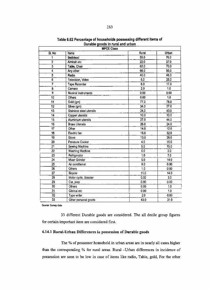
283
Table 6.62 Percentage of households possessing different items of ura e goo s In rura an ur an o bl d' Id b
MPCEClass SI. No Items Rural Urban
1 Bedstead 55.0 76.0 2 Almirah etc 22.0 37.0 3 Table, Chair 62.0 70.0 4 Any other 66.0 56.0 5 Radio 40.0 46.0 6 Television, Video 6.0 25.0 7 Tape. Recorder 6.0 17.0 8 Camera 2.0 1.0 9 Musical Instruments 0.00 0.00 10 Others 0.00 1.0 11 Gold (gm) 77.0 78.0 12 Silver (gm) 34.0 27.0 13 Stainless steel utensils 24.0 43.0 14 Copper utensils 10.0 13.0 15 Aluminium utensils 27.0 44.0 16 Brass Utensils 26.0 24.0 17 Other 14.0 12.0 18 Electric fan 15.0 32.0 19 Stove 13.0 26.0 20 Pressure Cooker 4.0 15.0 21 Sewing Machine 5.0 15.0 22 Washing Machine 0.0 2.0 23 Refrigerator 1.0 7.0 24 Mixer Grinder 5.0 14.0 25 Air conditioner 0.0 0.00 26 Others 1.0 0.00 27 Bicycle 11.0 14.0 28 Motor cycle, Scooter 0.00 3.0 29 Car, jeep 0.00 0.00 30 Others 0.00 to 31 Clinical etc 0.00 1.0 32 Type writer 2.0 0.00 33 Other personal goods 43.0 31.0
Source: Survey data.
33 different Durable goods are considered. The all decile group figures
for certain important item are considered first.
6.14.1 Rural-Urban Differences id possession of Durable goods
I
The % of possessor household in urban areas are in nearly all cases higher
than the corresponding % for rural areas. Rural -Urban differences in incidence of
possession are seen to be low in case of items like radio, Table, gold, For the other

284
durables listed in Table 6.65, the rural -urban differentials are much higher. Examples
are electric fan (rural 15%. urban 32%, stove rural 13% urban 26%).
6.14.2 Variation with over all level of living
Table 6.63: Percentage of households possessing different items of Durable , . goods in each MPCE class • rural
MPCEdass Items 0-200 200-400 400-600 600-800 >800 All Bedstead 53.6 44.4 65.0 60.0 83.3 55.0
.. Almirah etc 7.1 22.2 30.0 20.0 66.7 22.0 Table, chair 39.3 55.6 85.0 90.0 83.3 62.0 Any other 67.9 55.6 80.0 80.0 50.0 66.0 Radio 39.3 30.6 50.0 60.0 33.3 40.0 Television, Video 0.0 0.0 15.0 10.0 33.3 6.0 Tape Recorder 0.0 5.6 10.0 10.0 16.7 6.0 Camera 0.0 2.8 5.0 0.0 0.0 2.0 Musical Instruments 0.0 0.0 0.0 0.0 0.0 0.0 Others 0.0 0.0 0.0 0.0 0.0 0.0 Gold (gm) 67.9 72.2 85.0 90.0 100.0 77.0 Silver (gm) 32.1 41.7 30.0 20.0 33.3 34.0 Stainless steel utensils 17.9 16.7 30.0 40.0 50.0 24.0 Copper utensils 3.6 5.6 15.0 0.0 66.7 10.0 Aluminium Utensils 21.4 19.4 30.0 40.0 66.7 27.0 Brass Utensils 10.7 22.2 35.0 50.0 50.0 26.0 Other 7.1 5.6 20.0 30.0 50.0 14.0 Electric fan 3.6 0.0 35.0 40.0 50.0 15.0 Stove 0.0 5.6 30.0 10.0 66.7 13.0 Pressure Cooker 0.0 0.0 10.0 0.0 33.3 4.0 Sewing machine 7.1 2.8 5.0 0.0 16.7 5.0 Washing machine 0.0 0.0 0.0 0.0 0.0 0.0 Refrigerator 0.0 0.0 0.0 0.0 16.7 1.0 Mixer, Grinder 0.0 0.0 10.0 10.0 33.3 5.0 Air conditioner 0.0 0.0 0.0 0.0 0.0 0.0 Others 0.0 0.0 0.0 0.0 16.7 1.0 Bicycle 7.1 5.6 5.0 40.0 ·33.3 11.0 Motor, cycle, Scooter 0.0 0.0 0.0 0.0 0.0 0.0 Car,jeep 0.0 0.0 0.0 0.0 0.0 0.0 Others 0.0 0.0 0.0 0.0 0.0 0.0 Clinical etc. 0.0 0.0 0.0 0.0 0.0 0.0 Type writer 0.0 2.8 5.0 0.0 0.0 2.0 Other personal goods 39.3 50.0 45.0 30.0 33.3 43.0 Source: Survey data
Table 6.63 & 6.64 give the %s of households possessing each item of
Durable goods in each MPCE classes in rural and urban areas.

285
Variation with over all level of living is studied based on %s of
possessing households belonging to different ranges of household monthly per capita
consumer expenditure. Thus each of the five rural and urban MPCE groups contain
roughly same % of population both in rural and urban and may be thought of,
respectively, as the ' poorest' [in terms of level as reflected in the MPCE], the 'next
poorest', and so on up to the 'richest'.
Table 6.64 : Percentage of households possessing different items of Durable goods in each MPCE class- urban
MPr.F r.1~!':!':
Items 0-200 200-400 400-600 600-800 >800 Bedstead 61.5 64.7 80.0 82.4 100.0 Almirah etc 7.7 11.8 40.0 58.8 87.5 Table, chair 46.2 58.8 90.0 76.5 81.3 AAyother 46.2 35.3 60.0 58.8 100.0 Radio 30.8 38.2 55.0 64.7 43.8 Television, Video 0.0 8.8 10.0 41.2 81.3 Tape Recorder 0.0 2.9 15.0 29.4 50.0 Camera 0.0 0.0 0.0 0.0 6.3 Musical Instruments 0.0 0.0 0.0 0.0 0.0 others 0.0 0.0 0.0 0.0 6.3 Gold (gm) 61.5 70.6 80.0 82.4 100.0 Silver (gm) 15.4 17.6 45.0 29.4 31.3 Stainless steel utensils 61.5 41.2 20.0 29.4 75.0 Copper utensils 7.7 8.8 5.0 23.5 25.0 Aluminium Utensils 61.5 41.2 30.0 35.3 62.5 Brass Utensils 30.8 11.8 15.0 29.4 50.0 other 7.7 2.9 10.0 11.8 37.5 Electric fan 7.7 8.8 25.0 58.8 81.3 Stove 7.7 0.0 15.0 52.9 81.3 Pressure Cooker 0.0 0.0 5.0 17.6 68.8 Sewing machine 0.0 5.9 15.0 29.4 31.3 Washing machine 0.0 0.0 0.0 0.0 12.5 Refrigerator 0.0 0.0 0.0 5.9 ,37.5 Mixer, Grinder 0.0 0.0 5.0 23.5 56.3 Air conditioner 0.0 0.0 0.0 0.0 0.0 Others 0.0 0.0 0.0 0.0 0.0 Bicycle 15.4 8.8 25.0 11.8 12.5 Motor, cycle, Scooter 0.0 0.0 0.0 0.0 18.8 Car, jeep 0.0 0.0 0.0 0.0 0.0 Others 0.0 2.9 0.0 0.0 0.0 Clinical etc. 0.0 0.0 0.0 0.0 6.3 Type writer 0.0 0.0 0.0 0.0 0.0 other personal goods 15.4 17.6 40.0 41.2 50.0
Source: Survey data
All 76.0 37.0 70.0 56.0 46.0 25.0 17.0 1.0 0.0 1.0
78.0 27.0 43.0 13.0 44.0 24.0 12.0 32.0 26.0 15.0 15.0 2.0 7.0 14.0 0.0 0.0 14.0 3.0 0.0 1.0 1.0 0.0 31.0
I

286
The five ranges of MPCE to which the population of rural and urban areas
correspcnd are specified by their lower [or upper] limits. Here the object of interest is
the variation among the different MPCE groups in respect of the % of households
possessing each item of durable good s.
In figures 1-5 the % of households in .different MPCE class reporting
possession are shown graphically for five of the 33 Durable goods considered, with
the MPCE classes represented on horizontal axis.
Fiyunt u.; i.t:i~ul t: i.illlt: 11t:t:J~-!!/O of possessor households-Rural
100
90 80 -~ 70 - 60
:2 so j 40 ~
! 30 e 20 = 10
__ Radio
-4-Television, Video
--.-Tape Recorder L-_----.! ____ ---.J
i I
! 0
-10 0-200 200-400 400-600 600-800 >800
MPCEclass
Figure 6.10 Leisure time needs-% of possessor households-Urban
I I i
~I-'---Ra-d-io---II
-4-Television, Video! I --.-Tape Recorder J I
1
I 200-400 400-600 600-800 >800 I
lOO 90 - 80
~ 70 0 -:9 60 e SO .c::I ~ 40 ! 30 ~ 20
10
0
0-200
L-________________ M __ P_C_E_c_l_as_s __________________ ~ __ ~

287
6.15 Goods for leisure time needs:
Figures 6.9 and 6.10 show possession of goods for leisure time needs21
6.15.1 Radios
There is no marked contrast between rural and urban areas in the way the
incidence of possession varies over the MPCE Classes. For urban areas the curve
is seen to flatten out considerably. The % of possession in the lowest MPCE class is
30.8% . and in the highest 46%. In rural areas on the other hand the proportion of
possessor households in the lowest MPCE class is 39.3% and in the highest 40%. In
rural as well as urban areas a considerable %of households consider it as a leisure
time equipment that they can afford
6.15.2 Television and Video
There are much later arrivals on the Kerala market, compared, for the
instance, to the T.V.set. Incidence of possession in the lowest MPCE class is 0% and
highest MPCE class 33.3%in rural areas. The average for 'All' is only 6%. In the
urban sector for lowest MPCE class the % of possession is 0% and for highest MPCE
class is 81.3% Both commodities are clearly lUXUry items with the incidence of
possession rising sharply The incidence of possession curve rises sharply for upper
MPCE classes of urban sector as per NSSO data for general households. In urban
Kerala TV sets are possessed by nearly 15%_ofhouseholds in even the lowest MPCE
class and by nearly 50% households in the top MPCE class.
6.15.3 Tape Recorder
There is marked contrast between rural and urban areas in the way in
which incidence of possession varies over the MPCE classes for the urban areas the
curve is rising steadily as different from rural. The % of possession in the lowest
MPCE class is zero and in the highest 50% In the rural sector on the other harid the
proportion of possessor households in the lowest MPCE class is also zero and in the
highest MPCE class only 16.7 %.
6.15.4 Equipments for household work
Figures 6.11 and 6.12 gives possession of Equipments for household work.

288
6.15.5 Stoves
In the lowest MPCE class of rural population on3.6 % possessed stoves
and in the highest MPCE class 66.7%
100 90
- 80 ~ 0 70 -fIl 60 "0 50 -= .Cl 40 CII fIl 30 = = 20 = 10
0 -10
100
90
80 -~ 70 0 -- 60 ~ 50 -e .Cl CII
40 fIl 30 = e 20
== 10
0
-10
Figure 6.11 Labour saving Household equipment -% of possessor households-rural
I I i
r--+---St-o-ve----'j I
---Pressure Cooker
---.-- Sewing machine
-..<-Refrigerator
~ Mixer, Grinder
MPCE class
Figure 6.12 Labour saving Household equipment -% of possessor households-Urban
-+-Stove
---Pressure Cooker
---.-- Sewing machine
-+E- Refrigerator 11
~ Mixer, Grinder.J I
I !
0-200 200-400 400-600 600-800 >800
MPCE class
For urban areas figure 6.7 the variation in the % of possessing household is
not a totally different kind as in case of general households given in NSSO data. Starting
at a level of 7.7% for the lowest MPCE class, the % rise with each successive MPCE
class up to the 5th, at which point a peak (81.3%) is reached. The data thus enable one to
identity fairly accurately, the average level of living at which the stove, in urban Kerala,
begins to get substituted by "superior" equipment such as the LPG cylinder.

289
6.15.6 Pressure cookers
The % of rural possessor households is zero for the first two MPCE
classes of both rural and urban sectors. The incidence of possession then rises, ending
at 33.3% for the top MPCE class in rural and 68.8% for urban
6.15.7 Refrigerators
This commodity unmistakable luxury character not only for rural SC's
Kp.r~ht hut also for urban SC's. % of possessor households is of course much higher
in urban areas 37.5% for the highest MPCE class. In rural areas none of the
households possessed the item till the top most MPCE class where it is 16.75%
6.15.8 Sewing machine
In rural area the % of possessor households is higher [7.1%] for lowest
MPCE classes than urban [0 %]. For the highest MPCE class the % is 16.7 in rural
and 31.3 in urban. The curve is roughly linear and the propensity to possess a
machine increases only gradually with level of living,
6.15.9 Other durables
Figure 6.13 and 6.14 gives possession of other durables.
6.15.9.1 Electric Fans
The lowest MPCE class in rural sector has about 3.6 % households
possessing electric fans and the highest MPCE class 50%. The. incidence of
possession is very low for th~ lowest two MPCE classes but it goes up suddenly from
3rd MPCE class onwards The incidence of possession curve rises thereafter steeply.
The % of urban households with fans goes up from 7.7% for the lowest
MPCE class to 81.3for the highest, the slope of the incidence of possession curve
increases progressively as one move from lower to upper MPCE classes.

290
6.13 Electric fan, bicycles and two wheelers -% of possessor households-rural
so 40 30
20
I~t-~~::~~~~~~~~~ - \0 0-200 200-400 400-600 600-800 >lSVV
MPCEclass
-+-Bicycle
-4-Motor, cycle, Scooter
~ FJectric fan
6.14 Electric fan, bicycles and two wheelers -% of possessor households-urban
I ': 1
Il ~l i ~ so I CS
.c 40 1 ~ 30 1 :i3 20
10 o+-~--~~~-r--~ __ ==~~r-----'
-10 0-200 200-400 400-600 600-800 >800
MPCEclass
6.15.9.2 Motor cycles/Scooters
-+-Bicycle
-4-Motor, cycle, Scooter
----..- Electric fan
As per NSSO data the % of households with motorcycles or Scooters
raises smoothly in both rural and urban Kerala. In rural areas the % remains under 5%
up to the 9th MPCE class and then rises sharply to 24% for the highest MPCE class.
As per the sample data of rural SC's none of the SC households possessed the item
being an unreachable expenditure. In the urban sector possession of the item is
reported only for the top expenditure class [18.8 %]. This shows that even for urban
se's the item is a pure luxury.
6.15.9.3 Bicycles
The bicycle on the other hand is, a commodity affordable for many SC
households in rural as well as urban areas with the possession rate reaching a peak of 33.3
% for the top MPCE class in rural. In urban the % of possession increases from a minimum

291
of 15.45 to 25% for third MPCE class and then starts declining. The wban SC's consider it
as an 'inferior' item after they reaches a certain level of expenditure. In rural areas, by
contrast, the % of households with bicycles, rises from 7.15 % for the lowest MPCE class
and rises for each MPCE class and reaches 33.3% for the top MPCE class.
6.16 Average number possessed by households reporting possession
Table 6.65 and Table 6.66 shows for each 31 different Durable goods,
average number possessed by sample SC house holds in rural and urban areas. The
following features deserve mention.
Table 6.65 Possession of Durable goods by MPCE classes Rural
Items MPCEclass
0-200 200-400 400-600 600-800 >800 All Bedstead 1.3 1.7 2.2 2.0 3.0 1.9 Almirah etc 1.0 1.5 1.3 1.5 1.5 1.4 Table, chair 2.0 2.0 3.1 3.0 5.2 2.7 /vtyother 1.8 2.8 1.9 2.1 3:3 2.2 Radio 1.0 1.0 1.0 1.0 1.0 1.0 Television, Video - - 1.0 1.0 1.0 1.0 Tape Recorder - 1.0 1.0 1.0 1.0 1.0 Camera - 1.0 1.0 - - , 1.0 Musical Instruments - - - - - -Others - - - - - I -Gold (gm) 10.4 17.4 18.4 25.3 23.0 17.3 Silver (gm) 75.3 47.3 104.2 300.0 35.0 78.9 Stainless steel utensils 1.8 7.5 10.5 14.8 14.3 9.1 Copper utensils 1.0 6.0 1.0 - 2.3 2.5 Aluminium Utensils 1.2 1.9 4.0 7.5 4.5 3.4 Brass Utensils 1.3 1.3 1.6 3.0 2.3 1.8 Other 1.0 6.5 6.3 8.7 12.0 7.3 Electric fan 1.0 1.3 1.3 2.7 1.5 Stove - 1.0 1.0 1.0 1.0 1.0 Pressure Cooker - - 1.0 - 1.0 1.0 Sewing machine 1.0 1.0 1.0 - '1.0 1.0 Washing machine - - - - - -Refrigerator - - - - 1.0 1.0 Mixer, Grinder - - 1.0 1.0 1.0 1.0 Air conditioner - - - - - -Others - - - - 1.0 1.0 Bicycle 1.0 1.0 1.0 1.0 1.0 1.0 Motor, cycle, Scooter - - - - - -Car,jeep - - - - - -Others - - - - - -Clinical etc. - - - - - -Type writer 1.0 1.0 1.0 Other personal goods 1.5 2.3 2.6 2.7 2.5 2.2 Source. Survey data
I

292
The five ranges of MPCE to which the population of rural and urban areas
correspond are specified by their lower [or upper] limits. Here the object of interest is
the variation among the different MPCE groups in respect of the % of households
possessing each item of durable goods.
The five ranges of MPCE to which the population of rural and urban areas
correspond are specified by their lower [or upper] limits. Here the object of interest is
the variation among the different MPCE groups in respect of the % of households
possessing each item of durable good s.
Table 6.66 Possession of Durable goods by MPCE classes -Urban
MPCE class Items 0-200 200-400 400-600 600-800 >800 Bedstead 1.8 1.5 2.3 2.6 3.0 A1mirah etc 1.0 1.0 1.0 1.3 1.4 Table, chair 2.3 1.8 2.1 2.6 5.5 My other 1.5 1.3 1.9 2.4 3.4 Radio 1.0 1.0 1.0 1.0 1.0 Television, Video - 1.0 1.0 1.0 1.0 Tape Recorder - 1.0 1.0 1.0 1.0 Camera - - - - 1.0 Musical Instruments - - - - -Others - - - - 1.0 Gold (om) 12.4 11.1 25.8 40.7 77.1 Silver (gm) 23.0 29.2 41.3 68.4 34.8 Stainless steel utensils 6.3 6.9 10.0 20.2 24.8 Copper utensils 1.0 2.0 3.0 1.0 4.3 Aluminium Utensils 4.3 4.7 4.5 6.0 6.7 Brass Utensils 1.5 2.5 2.7 2.8 4.0 Other 10.0 4.0 6.0 7.0 9.5 Electric fan 2.0 1.0 1.4 1.5 2.4 Stove 1.0 - 1.0 1.0 1.4
• Pressure Cooker - - 1.0 1.0 1.7 Sewing machine - 1.0 1.0 1.0 1.0 Washino machine - - - - 1.0 Refrigerator - - - 1.0 1.0 Mixer, Grinder - - 1.0 1.0 1.0 Air conditioner - - - - -Others - - - - -Bicycle 1.0 1.0 1.0 1.0 1.0 Motor, cycle, Scooter - - - - 1.0 Car, jeep - - - - -Others - 1.0 - - -Clinical etc. - - - - 1.0 Type writer - - - - -Other personal ooods 1.0 1.3 1.8 3.0 2.6
All 2.2 1.2 2.8 2.3 1.0 1.0 1.0 1.0 -
1.0 33.1 41.1 13.6 2.4 5.2 2.9 8.1 1.8 1.2 1.5 1.0 1.0 1.0 1.0 --
1.0 1.0 -
1.0 1.0 -
2.1

293
The five ranges ofMPCE to which the population of rural and urban areas
correspond are specified by their lower [or upper] limits. Here the object of interest is
the variation among the different MPCE groups in respect of the % of households
possessing each item of durable good s.
The five ranges of MPCE to which the population of rural and urban areas
correspond are specified by their lower [or upper] limits. Here the object of interest is
the variation among the different MPCE groups in respect of the % of households
possessing each item of durable good s.
6.16.1 Furniture
Table 6.65 and 6.66 reveals that rural-urban differences are very less in
case of furniture. Among all items of furniture, almirah is the only item for which the
average number possessed by a rural SC household (1.41) is more than that in urban
areas (1.22). The average number of bedsteads, possessed by a rural household (1.85)
is less than that in urban areas (2.21). For other types of furniture, the average number
is more or less the same in two sectors.
6.16.2 TVNCRlVCP
Among the TV NCRlVCP owning households the average number of sets
owned was 1 in rural SC sample and the same in urban SC sample. This is low as
compared to the average possession of television and VCRlVCP sets for general
population in rural [1.03] and urban [1.05] Kerala as per NSSO data.
6.16.3 Radio
No variations are found in the average number of radio sets possessed by
household in urban (1.0) and rural (1.0) sectors.
6.16.4 Tape recorder
No variation in found in the average number of tape recorders possessed
by households in urban (1.0) and rural (1.0) sample areas The vast majority of
possessor households possessed only one and none of them possessed a second one.
294
6.16.5 Gold and Silver
Wide variations are observed in the average quantity of possession of
Gold and Silver in the rural and urban areas. se households possessed on an average
of 33.09 gms Gold in the urban sample area while rural sample se households
"possession was only 17.25 gms. Similarly regarding possession of silver rural se
households seen to be possessing more silver ornaments (78.91 grms) than urban
(41.07). The poor asset position of se households in the sample ar~as especially in
rural sector is revealed in this
6.16.6 Household utensils
While the average number of copper utensils possessed by rural se
households (2.50) exceeded that of urban (2.38) for all other types of household
utensils, the average number of possession per household was higher in urban areas.
Among household utensils stainless steel utensils was found to be used more by se's
both among urban and rural households.
6.16.7 Stove, pressure cooker
se households in the urban area reported an average of 1.19 stoves
possessed compared to (1) in rural areas. Implying that all possessor households in
rural sample possessed only one. In the urban sample the vast majority of possessor
households also possessed only one and less than 19 % owned a second one Average
number of pressure cookers possessed in urban area was 1.53. While in rural it was
(1) pressure cooker.
6.16.8 Mixer Grinder
Rural-urban difference was not found in the possession of mixer grinder.
Average possession of the item was equal (1) in both sample sectors.
6.16.9 Electric fan, Sewing machine
A household possessed 1.81 electric fan on an average in urban area while
the same in rural was 1.53.Regarding sewing machine number possessed was equal in
both sectors, (1) sewing machine.

295
6.16.10 Washing Machine, Refrigerator
While none of the sample se households possessed washing machine, the
urban average possession for those who possessed was (1) machine per household.
Both urban and rural areas reported equal average possession of (1) refrigerator.
6.16.11 Two Wheelers
Sample se households reported very low possession of personal vehicles a
household possessed 1 bicycle on an average in both rural and urban sample areas. Rural
sample households have not reported possession of any other two wheelers namely
motorcycles, Scooters etc. The only one which se's of sample rural area consider as
attainable is a bicycle. The average possession of Motorcycle and Scooter was (1)
For urban sample households neither rural nor urban households reported
possession of other vehicles such as car, jeep, etc.
6.16.12 Other personal goods
Among rural households the average household posseSSIOn of the
personal goods was reported to be higher (2.19) as compared to urban (2.13)
possession of the same.
6.16.13 Expenditure on Durable goods
Expenditure on durable for the sample popUlation as a whole, forms a
very small proportion of total household expenditure. Per capita household
expenditure on durables is estimated in the survey as only Rs.17.96 (4.82%) total
household spending in rural sector and Rs.68.80 (13.07%oftotal) in urban sector.

296
NOTES AND REFERENCES
1. Uma Ramaswami, (1984), "Preference and Progress. The Scheduled Caste",
Economic and Political Weekly, July 28,PP.12-14.
2. NSSO, (1996), "Survey Results on Level and Pattern of Consumer Expenditure",
based on NSS 50th round (July 1993-June 1994) data,May.
3. India, (1993(B», "Education of Scheduled Castes and Scheduled Tribes 1988-
·89", Department of Education, Government of India, New Delhi, 1989,Census of
India 1981 Controller of Publications, New Delhi.
4. Vagiswari, A, (1972), "Income Earning Trends and Social Status of the Harijan
Community in Tamil Nadu", Sangham Publishers, Madrass, P.11.
5. Jagadish, N, Bhagwati, (1985), "Wealth and Poverty", edited by Gene Grossman,
"Essays in Development Economics", VoU, Oxford University Press, Delhi,
P.178.
6. Note: Any other: Aged, Children, Unemployed.
7. Note: Other labourers includes: Construction workers, Household workers,
Headload workers and House wives.
8. Note: Employed: both in government sector and in private sector, the major
categories included are Engineer, Army, Teacher, Peon, Attender, Sweeper,
Thotty, Driver etc.
9. Note: Self Employed: Fish Selling, Beedi Making, Fire wood collection etc.
10. Survey of Income and Housing costs, Economic well being of households,
Australian bureau of statistics.
11. John Kenneth Galbraith, (1983), "The Voice of the Poor", Harward University
Press, Cambridge, P. 7 .
12. Note: Others: rented houses, layam or government accommodations free of
charge etc.
13. (a) Sharpe, I, Deanna,(1999), " Identifying poor and their consumption patterns",
University of Missouri, Columbia.

297
(b)Ghancy Abdel Muhanuned, (1999), "Family Economics and Nutrition
Review", Vo1.12,No.2, P.15.
14. NSSO, (1996), "Survey Results on Level and Pattern of Consumer Expenditure",
based on NSS 50th round (July 1993-June 1994) data, Report NoA02, May,
PP.to-lt.
15. NSSO, (2001), "Level and Pattern of Consumer Expenditure in India", 55th
round data, R~port NoA57, PP.38-41.
16. Note: Others: Students, Any other: Aged, Children. Unemployed.
17. Note: Unemployed or unable to work.
18. G.K.Nair,(2001), "Coconut Oil Increases Life Expectancy",
forumhub.comlsouthfoodl2693.05A4.html-12k, KOCH!, May 20.
19. Note: Other sources include from free collection from neighbors, forest
20. NSSO, (2002), "Survey Results On Level and Pattern of Consumer Expenditure
in India", based on NSS 55th round (July 1999-June 2000) data, Report
NoA57,Government of India,P.7.
21. Leisure time needs: Radio, Tape recorder, Television, Video.

CHAPTER 7
FINDINGS AND RECOMMENDATIONS
~ore than half a century has elapsed after India attainted independence.
Ever since then our National leaders and the successive Governments have brought
about a number of reforms with the specific objective of alleviating the poverty of the
downtrodden masses especially the backward communities. Despite all these efforts
we find that even now they continue to remain marginalized from enjoying the fruits
of development. Even in a State like Kerala which boasts of a unique development
experience, with social indicators like literacy birth rate, death rate and health status
being comparable to countries like U.S.A, the scheduled castes, especially those
living in the rural areas are still experiencing standards of living much below that of
the general popUlation. In this context, the present study made an attempt to analyse
the socio-economic background and the consumption pattern of scheduled caste
households in Idukki district. The summary of the findings on various aspects and
recommendations of the study are given in this chapter.
A comparative study of the MPCE of Scheduled castes in India and
Kerala with that of General households in India and Kerala using NSSO data has
brought out the following features:
7.1 Distribution ofMPCE among scheduled Castes
Looking to the proportion of persons in each MPCE level, it is found that,
the MPCE position of schedules castes popUlation in rural Kerala is lower than that of
the general popUlation. This is the same trend at all India level. The MPCE position
of SC's in urban Kerala is also lower than that of general population in Kerala.The
same trend is found at the all India level. However the MPCE position of rural Kerala
SC's is better than that of SC's in rural India. The MPCE position of urban Kerala
SC's is also higher than that of SC's in urban India. More percentage of SC
popUlation in rural Kerala fall in lower MPCE levels than urban SC's. Similarly in
rural India more percentage ofSC's fall in lower MPCE classes than urban SC's ..

299
Looking in to the distribution of persons in to different MPCE classes. It
is found that MPCE position of se households in both rural and urban Kerala is
lower than that of non-Sc households in both sectors in both Kerala and India. MPCE
position of SC's in both rural and urban Kerala is better than that of SC's in the All
India level. More percentage of SC's fall in lower MPCE ranges in rural Kerala than
Urban Kerala. Similuc is the trend in all-India also.
7.2 Size distribution of Scheduled Castes
Looking to the average size oi ~C households it IS tound that, In case of
rural Kerala for SC's average household size is higher than (5.24) the urban SC's
(4.75).All India level also rural SC's have larger household size (4.85) than urban
SC's (4.75).Average size of rural SC households in Kerala is higher than rural SC
households in All India. Average household size of urban SC households in Kerala is
higher than All India urban SC's. Average household size is higher in rural sector for
SC's in Kerala as well as all-India.
7.3 Proportion of Expenditure on food of SC's
Analysis of proportion of expenditure on food for scheduled Castes
provided the following findings: For rural Kerala SC's percentage expenditure on
food declined from 1983to 1987-88.Same trend is found for food expenditure in all
India also. For rural India SC's percentage expenditure on food declined from 1983 to
1993-94.Food expenditure for Kerala urban SC's declined from 983 to 1987-88.In
case of urban India SC's percentage expenditure on food declined from 83 to 93-94.
Here it is observed that the pattern similar to that of general households.
In rural Kerala for general households, percentage expenditure on food
declined from 1983 to 1987-88.In rural India for percentage expenditure on food
declined from 1983 to 63.23 in 1993-94 .. For urban Kerala general households the
percentage expenditure on food increased from 1983 to 1987-88.For urban India
general households the percentage expenditure on food changed only very little
between 1983 to 1987-88. But there was a steady decline between 1987-88 and 1993-
94.So it is found that as in case of the general households in Kerala as well as in India

" 300
percentage of expenditure on food of scheduled castes was declining between 1983-
1993-94.
7.4 Pattern of Consumption Expenditure of SC's.
It is found that (considering all expenditure classes) average MPCE of ,
SC's in rural Kerala is lower than that on general households). This is similar to the
situation of SC's and general households of all India rural sectors. In the top most
MPCE classes of Rs.300& above the average MPCE of SC's found very high in
Kerala. At All- India level in the top most MPeE classes of Rs.300& above the
average MPCE of SC's is greater than that of general households
Unlike the pattern of MPCE for the total popUlation of SC's, the top
expenditure class among Sc' s exhibit close similarly in average MPCE to the general
population in rural India. In the top expenditure class in rural average MPCE is lower
and MPCE on food is higher for general households That is the average MPCE is
higher and MPCE on food is lower for SC's in the top expenditure class. SC's
belonging to top expenditure class spend morethan general households on food items
like cereals, fish and egg and on non-food items like pan, tobacco and intoxicants,
miscellaneous goods and services and durable goods in rural India. SC's in rural India
spend less than general households on food items like pulses, milk and milk products,
fruits and nuts, beverages and refreshments and non-food items like clothing and
footwear in the top expenditure class. Considering all expenditure classes, average
MPCE of SC's in rural and urban Kerala and India is lower than that of general
households. Considering " top expenditure class" in rural and urban sector average ")
MPCE of SC's jn higher than general households on items such as cereals, meat, fish
and egg and non-food items like pan, tobacco and intoxicants, miscellaneous goods
and services and durable goods.
7.5 Per capita Expenditure.
As observed earlier average monthly per capita expenditure general
households of Kerala is found much higher than that of SC's of rural and urban
Kerala. In urban Sc's spend on food 63.08% on food and general households spend

301
5938%SC's non-food expenditure in rural Kerala was 33.48% of total MPCE and
that of general households 38.33%. The same trend was seen in urban also. MPCE on
cereals of Sc's of rural Kerala was higher than that of general households in rural
Kerala. In urban Kerala also same trend. SC's had higher average MPCE only on
cereals, and spices in rural Kerala than general households urban SC's have higher
average MPCE on sum more items sugar, and beverages and refreshments than non
SC's in urban Kerala. Among non-food in rural and urban Kerala SC's have higher
expenditure on only two items pan, tobacco and intoxicants, fuel and light. It is found
that Sc' s in both rural and urban Kerala have higher percentage expenditure on food
than general households Among food items cereals, cereal substitutes and spices are
the item that lead in the food basket of SC's than general households MPCE on non
food items pan. Tobacco and intoxicants and fuel and light exceed that of general
households in both rural and urban Kerala.
7.6 Movement in budget Share
Analysis of movement in the budget share for SC's over the period using
NSSO data 1983- 1993-94 showed that over the period from 1983- 1987-88,
expenditures have increased an all items for SC's in both Kerala and ali India rural
and urban. Proportion of expenditure on food declined while that of non-food has
increased. In food group in rural and urban items attracting more expenditures were
cereals, beverages and refreshments, meat, egg and fish and spices·. Percentage
expenditure on clothing is found to be declining while expenditure on footwear is
increasing in both sectors. In urban sector percentage of expenditure on durable goods
found decreasing during the period, and increasing in rural sector. Per capita
expenditure on the item was found less than that in rural sector.
7.7 Percentage expenditure of SC's
Looking to the percentage expenditure over the years for Kerala, it is
found that for SC's expenditure on cereals is declining over the period in both rural
and urban Kerala Similar trend s found in all India level percentage expenditure on
cereals declined steadily during the period. Increase in percentage expenditure has
been observed in case of durable goods. Increase in percentage expenditure has been
302
seen for all India SC's in rural and urban for durable goods. Expenditure on clothing
in total non-food expenditure in declining for SC's in rural sector of Kerala and
increased in urban Kerala. At all India level also clothing expenditure has been
declining for SC's.
7.8 Per capita consumption expenditure.
Looking to per capita consumption expenditure it is found that average
MPCE of SC's lower than that of general households in rural Kerala. Same trend is
tound in rural India also. In urban Kerala also average MPCE of SC's is lower than
that of general households same trend is found in urban India also.
7.9 Rliral Urban differences Kerala Consumption Pattern
Examinations of consumption pattern of rural and urban Kerala for
Scheduled castes show significant changes. In rural sector, footwear, durable goods
and total non-food are found to be consumed at an increased rate. In urban
consumption of durable goods is fast increasing. Cereals expenditure is declining for
rural SC's of Kerala. Clothing expenditure is declining for rural and increasing for
urban. In both rural and urban Kerala for SC's expenditure ratio of food and non-food
items changed showing decrease in food consumption and an increase in non-food
consumption. Similar trend is found in all-India also expenditure ratio of food and
non-food items has changed. Non-food consumption of SC's in Kerala rural SC's
higher than that of rural India SC's. For durable goods SC's in urban Kerala have
lower expenditure than urban all India SC's.
7.10 MPCE among Occupation groups.
Higher proportion of population in lower MPCE classes is seen among
labour households (agricultural labour, other labour) than all households in Kerala.
Similar trend is seen in rural India also MPCE levels casual labour households were
lower than other categories of households in urban Kerala.In urban India also same
trend has been observed MPCE among Occupation Groups for SC's. Estimation of
the two lowest and two top MPCE classes brings some important differences. At the
all India level it is found that SC's is more affected by poverty than "others" in each

303
occupation category. Incidence of poverty is more pronounced among agricultural
labour households among SC's. in the lower tail of MPCE distribution. In the upper
tail of MPCE distribution, differences among SC's is most prominent for "other type"
households.
Analysis of the consumption expenditure pattern and socio-economic
background of sample Scheduled Caste households gave the following findings.
1. The scheduled casts living in the rural sample of Idukki district belong to five
types of occupational categories viz, Agricultural labourers (17.87%) Other
labourers (25.11%), Farmers (1.70%), Regular salaried (9.15%) and Self
employed (2.98%). Percentage of unemployed in the rural sample is 8.51.
Students constituted 9.36% in the rural sample.
The scheduled caste living in the urban sample of Idukki district are engaged in
four types of occupations viz; Agricultural labourers (10.19%), Other labourers
(27.01 %), Regular salaried (17.54%) and Self employed (1.66%). The
percentage of 'others' is found to be much high among SC's.
2. Among the rural sample SC house holds literacy rate is 91 % and in the urban
sample it is 84%. There is 3.2% male illiteracy and 6.2% female illiteracy among
sample rural SC's of Idukki district. In the urban sample the male illiteracy is
3.3% and female illiteracy is 13.3%.
3. 20.9% of rural sample and 17.3% of urban sample have "below standard V",
level of education. 55.5% of rural sample and 50.5% of urban sample SC's have
education level "Standard V - Standard X".
4. Only 3.1 % of rural SC's and 13.5%"of urban SC's in sample area belong to an
educational level of "above SSLC".
5. Average household size of rural sample is 4.7 and that of urban sample 4.22.
Rural household size ofSC's is higher than urban household size. At the all India
level and for Kerala state average household size of SC's in rural sector is found
higher than that of urban SC's.
6. Average monthly per capita income of rural sample SC's (Rs.450) is lower than
the same for urban sample (Rs.634.4)

304
7. Average monthly per capita expenditure of rural sample SC's households
(Rs . .372.57) is found lower than the same for urban sample (Rs.526).
8. Average monthly per capita savings among sample SC households is very less;
lower in rural sample (Rs. 78.42) than in urban sample (Rs. 93.33).
Among sample in SC households in both rural and urban more percentage of
households fall in lower Monthly Per Capita Consumption Expenditure (MPCE)
classes as similar to the trend found between SC's in all India and all Kerala
9. The f'errent~gf" 0f sr hn11~ph0~t1~ in the MPCE class of above Rs. 355 (top
MPCE class) is higher for urban sector in Kerala (50%) than in rural sector
(20%).
10. In the top most MPCE class at all India level for SC's, the average MPCE
(Rs.448) is greater than that of general population (Rs. 445). The same trend is
found in Kerala also. This could be because they have been able to avail the
concessions offered to them, while the people in the lower MPCE classes may not
even be aware of these issues.
11. Also for the SC's belonging to the top most MPCE class in the sample rural and
urban areas have high average MPCE.
12. Unlike the pattern of MPCE for the total of SC's, the top expenditure class
among them exhibits close similarity in their average MPCE to the general
popUlation in all India and Kerala.
13. For the sample SC households in both rural and urban, proportion of food in total
expenditure is higher for lower expenditure classes and proportion of non-food
higher for higher expenditure classes as already established by theory.
14. At all India level, SC's in the top expenditure class spend more than general
households on food items such as cereals, meat, fish and egg and non-food items
like pan, tobacco and intoxicants, miscellaneous goods and services and durable
goods. They spend less than general households on food items such as pulses,
milk and milk products, fruits and nuts, beverages and refreshments and non
food items such as clothing and footwear.

305
In Kerala SC's in both rural and urban have higher percentage expenditure on
food, than general households. MPCE on pan, tobacco and intoxicants of SC's
exceeded that of general households in both rural and urban Kerala which is one
reason why they have not been able to rise up from the low standards ofliving.
15. For the sample rural SC's MPCE on food constituted 56.88% and in urban
45.46%. MPCE on non-food of sample SC's in rural constituted 43.12% where as
in urban areas it was 54.54%. Those SC's living in urban areas have adapted the
life styles of the other communities and have more or less merged in to the main
stream of the community.
16. Significant differences are there in the "total expenditure" and "expenditure on
non-food items" between SC's in rural and urban samples in the study area.
17. Mean coru:umption of food is not significantly different in rural and wban sample
area.
18. Over the period from 1983 to 1993-1994 for all India and Kerala expenditures
on all items have increased for SC's in both sectors.
The proportion of expenditure on food declined and that of non-food increased for
SC's during the period. Percentage expenditure on cereals is found declining over
the period.
19. Top most MPCE classes among rural and urban SC households in sample area
show preference towards non-food expenditure and conspicuous consumption
which is in line with the general pattern of behaviour.
20. Total expenditure of SC households consisted of consumption .out of cash
purchases; home grow stock, gift loan and free collection.
21. Results of X2 test revealed that there is significant association between monthly
per capita expenditure and income, education, occupation and place of residence
for SC's in sample area and this finding supported the third hypothesis.
It was found that higher MPCE levels are associated with higher income, higher
levels of education, better occupational status and residents in urban areas.

306
22. ·Results of regression analysis using double log model showed that there is
significant differences in the .consumption elasticity of different items among SC
households in the study area. This finding supported the initial hypothesis of the
study.
23. Significant differences exist in the consumption pattern of poorer ~d richer
segments of SC population in the sample area. Average MPCE on food and non
food items by SC's belonging to different decile groups showed disparities in the
distribution of MPCE. This finding has supported the second hypothesis of the
study.
7.11 Recommendations
The study has found that the levels of livings of the Scheduled Castes are
far below the expectations. Large percentage of the Scheduled Caste belongs to low
income groups.· This is due their very low economic status and the consequent
employment prospects in low paying occupations. The consumption standards of the
majority of Scheduled Castes are found to be much below that of General popUlation.
Effective implementation of the Schemes for their economic upliftment is needed for
improving their consumption standards
Some of the scheduled castes have a comparatively better status in
educational field. But the educational attainments of the Scheduled Castes especially in
the rural areas are much below that of General popUlation. Hence the present
educational concessions to Scheduled Castes should be continued wherever necessary.
The analysis of the occupation distribution of Scheduled Castes has revealed
a very dismal picture even after five decades of programmes for their upliftment. For
their economic upliftment a change in their occupational pattern is necessary. The
Minimum wage Act in the case of agricultura1labourers should be enforced.
In the agricultural sector the contribution of Scheduled Castes is mainly
as agricultural labourers. Their participation as cultivators is handicapped by the non
availability of cultivable land. For those few cultivators among them the lack of
resources is the main hurdle in developing their land. As the educational attainment of

307
a majority of Scheduled Castes are very iow the bulk of the population should be
provided employment in other fields. The sectors, which can absorb them. are the
agricultural and small industries sector. There are a few hailing from households
pursuing traditional and cottage industries. Regarding the case of Scheduled Castes in
Idukki district this is very important. Facilities for enlarging their activity should be
provided; others should be given employment in the agricultural sector.
Schemes for improving the health standards of women and children
among Scheduled Castes is necessary to improve their consumption standards.
Majority of the Scheduled castes having low educational status are either not aware or
are careless of the importance of better health standards. Hence they are found to be
addicted to pan, tobacco and drugs and intoxicants, which adversely affects not only
their health but also hinders their economic progress. This also adversely affects the
consumption standards of the other members ofthe households.
The housing conditions of the Scheduled castes in the study area are
found to be deplorable both in rural and urban sectors. Even though the Government
has implemented various schemes they have not been properly utilized and hence
programmes for creating better awareness regarding the schemes should be provided.
Besides the colonization programmes should be extended to the unreached areas and
the existing facilities in the colonies should be improved.
Lack of availability of enough State level data on the status of scheduled
castes and also on different sub-castes is a major problem in studying the conditions
of Scheduled Castes in Kerala. An intensive data collection on the various socio
economic aspects of Scheduled Castes is necessary to help the researchers in the field.

BIBLIOGRAPHY BOOKS
1. Andre Betelle, (1971), University of California Press, Berkeley.
2. Allen. R.G.D and Bowley, A.L, (1935), "Family Expenditure-A study of its
variations", London, Staples Press.
3. Bharadwaj, A.N, (1979), "Problems of Scheduled Castes and Scheduled Tribes
in India", P .11.
4. Chatterjee, G.S, etal, (1974), "Poverty and Income Distribution", Statistical
Publishing Society, P. 150.
5. Celestin BougIe, (1971), "Essays on the Caste System", Cambridge University
Press.
6. Celestin BougIe, (1971), "Essays on the Caste System", Translated by Pocook,
D.F, University of Sussex, P.148.
7. Deaton Angus (2000), "Poverty and inequality in India: A Re-Examination in the
1990's".
8. Dandekar, V.M and Nilakantha Rath, (1971),"Poverty in India-f', Dimensions
and Trends, January, PP.25-47.
9. Devenant, C, (1699), "An Essay Upon the Probable Methods of Making a People
Gainers in the Balance of Trade", London.
10. Deaton Angus and Muellbauer John, (1980), "Economics and Consumer
Behaviour", Cambridge University Press, London, Chapters 2,3 and 8.
11. Dumont, L,( 1970), "H.:>mo Hierarchy The Caste and its Implications", London.
12. Evans, M.K, (1969), "Macro Economic Activity Theory of Forecasting and
Control", An Econometrica Approach, Harper and Row, New York, Evanston
and London.
13. Gandhi, M.K, (1945), Yeravada Mandir, Ahmedabad, Chapter IX.
14. Gupta Anil, (1986), "Consumption Behaviour in India- A Study of All India
Consumption Estimates", Anmol Publications, Delhi, P.12.
15. Jagadish, N, Bhagwati, (1985), "Wealth and Poverty", edited by Gene Grossman,
"Essays in Development Economics", VoLl, Oxford University Press, Delhi,
P.178.
16. John Kenneth Galbraith, (1983), " the Voice of the Poor", Harward University
Press, Cambridge, P. 7.
309
17. Kunhaman, M, (1989), "Development of Tribal Economy Development of
Underdeveloped". Classical Publishing Company, New Delhi.
18. Keynes, J. r,,1, (1936), <'The General Theory of Employment Interest and
Money", Harcourt Brace, New York, P.96.
19. King, G, (1936), "Natural and Political Observations and Conclusions Upon the
State and Condition ·of England (1696) in two Tracts", by Gregory King(ed),
Bamett, G.E, Johns Hopkins Press, Puttimore.
20. Lloyd, G.H, (1771), "An Essay On the Theory lIfMoney", London.
21. Mahajan, B.M, (1983), "Consumer Behaviour in India- An Economic Study",
Concept Publishing, New Delhi, P.151.
22. More Galander, (1984), "Competing Equalities: Lwa and the Backward Classes
in India", Oxford University Press, Delhi, P.18.
23. Modigliani, F and Ando, A, (1960), "The Permanent Income and the Life Cycle
Hypothesis of Savings Behaviour Comparisons and Test", in Friend, I and Jones,
R, (eds), Consumption and Savings, Vo 1. 11, University of Pennsylvania Press,
Philadelphia, P.126.
24. Modigliani, F and Brumberg, R, (1954), "Utility Analysis and the
Consumption Function an Interpretation of Cross Section data", in Post
Keynesian Economics, (ed) Kurihara, K.K, Rutgers University Press.
25. Milton Friedman, (1957), "A Theory of Consumption Function", University of
Chicago.
26. Oommen, T.K, (1984), " Social Transformation in Rural India-Mobilisation and
State Intervation", Vikas Publishing House, New Delhi, P.118.
27. Premchand, (1962), "Vividh Prasang", VoUI, Allahabad,P.471.
28. Prais, SJ and Houthakker, H.S, (1971), "The Analysis of Family Budgets", (2nd
impression)~ Cambridge University Press, Cambridge.
29. Paswan Sanj ay, etal, (1999), "Encyclopedia of Dalits in India", Social Justice,
Vo1.7, PP. 11-45.
30. Paswan Sanjay, etal, (1999), "Encyclopedia of Dalits in India", Struggle for Self
Liberation, Vo1.2.
31. Paswan Sanjay, etal. (1999), "Encyclopedia of Dalits in India", Social Justice,
Vol.4.
32. Roger, S, Mason, (1981), "Conspicuous consumption", Gower Publishing
Company Limited, England, P.18.
33. Ravallion Martin, (1990), "Economic Development and Cultural Change"

310
34. Roy and Laha, (1954), "A Study of Consumption Pattern in India".
35. Saradhamani, K, (1981), "Study (If Kerala Village", Ajantha Publications.
India, New Delhi.
36. Srinivas, M.N, (1997), "Caste In Modem India and Other Essays", Asia
Publishing House, Bombay.
37. (a) Sharpe, I, Dear'1a, (1999), " Identifying Poor and their Consumption
Patterns", University of Missouri, Columbia.
(b) Ghancy Abdel Muhammed, (1999), .. Family Economics and Nutrition
Review", Vo1.l2, No.2, P.15.
38. Stone J.R.N, (1954(a», "The Measurement of Consumer Expenditure and
Behavior in the United Kingdom, 1920-1938", YoU, Cambridge University
Press, Cambridge.
39. Sooryamoorthy, R, (1997), "Consumption to Consumerism-In the Context to
Kerala", Classical Publishing Company, New Delhi, P.50.
40. Sinha Surjit, (1968), "Caste in India-Its Essential Pattern of Socio-Cultural
Integration, In Caste and Race: Comparitive Approach", edited by Antony Reuck
and Julie Knight, I and Church Hill, A, Ltd, London.
41. Slutsky, E, (1915), "Sulla Teoria Del Bilancio Del Consomatore", Giomale
Degli Economisti, Vo1.51 [English translation by Stigler, G.J and Boulding, K.E,
(eds), (1952), "Readings in Price Theory", Chicago University Press.
42. Schultz, H, (1938), "The Theory and Measurement of Demand", Chicago
University Press.
43. Samuelson, P.A and William, D, Nordhaus, (1995), "Economics", Mc Graw Hill,
INC, P.73.
44. Timbrell, M.C, (1976), "Consumption Functions", in Topics. in Applied Macro
Economics, Eds David, Health Field, P.167.
45. Vaidyanathan, A, (1974), "Some Aspects of Inequalities in Living Standards in
Rural India", Poverty and Income Distribution, Statistical Publishing Society,
Culcutta, PP.215-241.
46. Vagiswari, A, (1972), "Income Earning Trends and Social Status of the Harijan
Community in Tamil Nadu", Sangham Publishers, Madrass, P.ll.

311
JOURNALS
1. Ando, A and Modigliani, F, (1963), "The Life Cycle Hypothesis of Savings,
Aggregate Implications and Tests", American Economic Review, Vol.S3, No.1.
2. Bardhan, (1970), "On Minimum Level of Living and Rural Poor India",
Economic Review, Vol.V, (New Series).
3. Ball, R.J and Drake, P.S, (1964), "The Relationship Between' Aggregate
Consumption and Wealth", International Economic Review, Vol.53, No.l,
January, PP.55-84.
4. Bodkin, R.G, (1959), "Windfall Income and Consumption", AmericariEconomic
Review, Vo1.49, No.4, September, PP.602-614.
5. Behrman, R, Jere and Deolalikar, (1987), "A Case of Study for Rural South
India", Journal of Political Economy, Vol.95, No.3, PP.492-507.
6. Berchanhall, C.R, et. ai, (1989), "A Seasonal Model of Con:sumption", The
Economic Journal, September, PP.837-843.
7. Bernoulli, D, (1738), "Specimen Theoriae Novae De Mensura Sortis",
Commentori; academic Scientiarum Imperialis Petropolitance". [English
translation by Sommer, L (1954),"Exposition of a New Theory on the
Measurement of Risk", Econometrica, Vol.22.
8. Brady, D.S and Friedman, R.D, (1947), "Savings and Income Distribution", In
Studies in Income and Wealth, Vol.XV, National Bureau of Economic Research,
New York.
9. Brown, T.M, (1952), "Habit Persistence and Lags in Consumer Behaviour",
Econometrica, Vol. XX, No.3, PP.335-371, July.
10. Beegom Javernesa, M.J, (1985), "Aiyankali and the Social Awakening among
the Pulayar", Jow.nal ofKerala Studies, Vol.XII, Parts. 1-14, PP. 11-21.
11. Burney A Nadeem et. ai, (1992), "Household· Size, its Composition and
Consumption Patterns in Pakistan: An Empirical Analysis Using Micro Data",
Indian Economic Review, Department of Economics, Delhi School of
Economics,Vol. 27, Issue. 1, July, PP. 57-72.
12. Bharat Patnakar and Gail Omvedt, (1979), "The Dalit Liberation Movement in
Colonial Period", Economic and Political Weekly, Vol. XN, No.8, PP.411-4l3.
l3. Chakravarthy, S.K and Pattnaik, R.R, (1970), "Income Distribution and Saving
and Investment Pattern of Cultivating Households; A Case Study of Orissa",
Indian Journal of Agriculture Economics, Vol.25, No.3, Bombay, PP.99-11 O.
312
14. Dissanayake Mallika and Files, (1988), "Household Expenditure in Srilanka an
Engel Curve Analysis", 10urnai of Quantitative Economics, YoLlV, No.l,
January, PP.133-155, PP.117-137.
15. Davis, T.E, (1952), ·'The Consumption Function as a Tool For Prediction ",
Review of Economics and Statistics, Vo1.34.
16. Friend, I and Kravis, I.B, (1957), "Consumption Pattern and Permanent
Income", American Economic Review, Papers and Proceedings, May.
17. Farre!, M.J, (1959), "The New Theories of Consumption Function ", Economic
Journal, Vo1.69, PP.678-696.
18. Gandhi,M.K(1966), "Collected Works", XX,April-August 1921,Govemment
of India ,Navjivan
19. Houthakker, H.S, (1950), "Revealed Preference and The Utility Function",
Economica, Vo1.17.
20. Houthakker, H.S, (1961), "The Present State of Consumption Theory",
Econometrica, Vo1.29.
21. Houthakker, H.S, (1957), "An International Comparison of Household
Expenditure Patterns Commemorating the Centenary of Engel's Law",
Econometrica, Vo1.25, No.4, October, PP.532-551.
22. Iyengar, N.S, (1960), "On a Method of Computing Engel Elasticities from
Concentration Curves", Econometrica, Vo1.28.
23. Johar, R.S, Sandhu, (1982), "Consumption Pattern in Panjab", Indian Economic
Journal, Vo1.29, No.4, April-June, PP.69-85.
24. Klein, L.R, (1958), "The Friedman-Becker Illusion", Journal of Political
Economy, Vo1.66, No.6, December, P.54.
25. Kannan, K.P, (1990), "Kerala Economy at the Cross Roads", Economic and
Political Weekly, September, P.1951.
26. Kozel,Valerie et.al,(1999)A Profile and Diagnostic of Poverty In Uttar
Pradesh,Economic and Political Weekly ,January .25-31,2003,P.301.
27. Leser, C.E.V, (1963), "Forms of Engel Functions", Econometrica, Vo1.31 , No.4,
October, PP.694-703.
28. Mayor, T, (1966), "The Propensity to Consume Permanent Income", American
Economic Review, Vo1.56, ~0.5, December, PP.1158-1177.
29. Mukhopadhya, Rabindranath, (1987), "A Study of Regional Patterns of
Consumer Expenditure in Rural India", Journal of Quantitative Economics,
Vo1.lll, No.!, January.

313
30. MukheIjee. M and Chatterjee, G.S, (1967), "Trends in Distribution of National
Incomes 1950-51 to 1965-66", Economic and Political Weekly, July .
.3 L Minhas, B.S. (1970), "'Rural Poverty Land Redistribution and Development",
Indian Economic Review, Vol.V, (New Series).
32. Mahajan, B.M, (1971), "Inter-Regional Homogeneity of Consumer Behaviour in
India", Arthavijana, Vol.XIII, No.l, March, PP.I-5I.
33. Murthy, G.V.S.N, (1971), "Pattern of Consumer Expenditure In Gujatat",
Anvesak, YoU, ~ecember, PP.175-183.
34. Mehta, B. C, (1971), "Analysis of Consumption Pattern in Rajasthan",
Arthavikas, Vol, XV, NO.!, Sardhar Patel University, Vallabh Vidhya- Nagar,
Gujarat, PP.56-65.
35. Maiti Pradip, etal, (1993), "Trends in Level of Living in Urban India", Economic
and Political Weekly, November, PP.2547-2550.
36. Majeri, K, Mustafa, etal, (1993), "Consumption Savings and Investment by
Social Class in Bangladesh: Does the Rural Sector Support the Urban Sector?",
The Journal of Development Studies, Vol.30, No.l, October, PP.226-245.
37. Nayak Vijay and Prasad Shailaja, (1984), "On Levels of Living of Scheduled
Castes and Scheduled Tribes", Economic and Political Weekly, July, PP.1205-
1213.
38. Navajivan, (1924), Vol.XXIV, June 29,P.321 and in Young India (1925), CWMG,
Vol.XXVI, February 5, P.73.
39. Navajivan, (1924), Vol.XXIV, May.18, P.40.
40. Panicker, P.G.K, (1979), "Employment Income and Food in Take among
Agricultural Labour Households", Economic and Political Weekly, Vol. XIV,
No.34, Bombay, Pp.1464-1470.
41. Pendakur Krishna, (2001), "Consumption Poverty in Canada, 1969 to 1998",
Journal of Canadian Public Policy, University of Toronto Press, Volume. 27,
Issue. 2, June, pp 125-149.
42. Radhakrishna, R and Atul Sarnla, (1975), " Inflation and Disparities in the Level
of Living-Indian", Economic Journal, April-June, PP.364-373.
43. Rajuladevi,A.K.(2001), "Food Poverty and Consumption among Landless
Labour Households", Economic and Political Weekly ,July,P.2656.
44. Szuk Adam, (1980), "Measurement of Poverty: Poland in the 1980's:" Review of
Income and Wealth.

314
45. Saggar Mridul, (1994), "Scheduled Castes and Scheduled Tribes in Eastern
India", Economic and Political weekly, March, PP.567-574.
46. Saha Somesh, (1980), "Some Further Estimates of Engel Elasticities for Rural
and Urban India", Sankhya, D, The Indian Journal of Statistics 1980,Vo1.42,
Series-D, Pts. 1 and 2.PP.127-150.
47. Sen Rajkumar, (1990), "The Changing Pattern and Distribution of Consumption
Expenditure in India", Rabindra Bharathi University, Calcutta, P.232.
48. Sharma, L.R, (1982), "Poverty and Inequality in the Rural Sector of Himachal
Pradesh", Economic AtTaires, Vo1.27, No.7-9, Calcutta.
49. Sawant, S, D, (1982), "Incidence of Under Nutrition in Rural India. An Inter
regional Perspective", The Indian Economic Journal, Vo1.29, No.4, April-June,
PP. 19-49.
50. Stone Richard, (1954), "Linear Expenditure Systems and Demand Analysis, An
Application to the Pattern of British Demand", The Economic Journal, Vo1.64,
September, PP.511-527.
51. Saradamani, k, (1981), "Education, Employment and Land Ownership: Role of
Caste and Economic Factors", Economic and Political weekly, VoI.XVI, No.
36,PP.1466-1469.
52. Saggar Mridul and Pan Indranil, (1994), "Scheduled Castes and Scheduled
Tribes in Eastern India Inequality and Poverty Estimates", Economic and
Political Weekly, March, PP.567-574.
53. Samuelson, P. A, (1938), "A Note On the Pure Theory of Consumer Behaviour",
Economica. VoLS. ,
54. Samuelson, P. A. (1950), "The Problem of Integrability in Utility Theory",
Economica, VoL 17.
55. Stigler, G.J, (1954), "The Development of Utility Theory", Journal of Political
Economy, Vo1.62.
56. Stone, J.R.N, (1954(b», "Linear Expenditure System and Demand Analysis, An
Application to the Pattern of British Demand", The Economic Journal, Vo1.54,
PP.511-527.
57. Smithies, (1945), "Forecasting Post-War Demand", Econometrica, VoU3.
58. Theil, H, (1965), "The Information Approach to Demand Analysis",
Econometrica, Vo1.33, No, I,PP.67-87.
59. Uma Ramaswami, (1984), "Preference and Progress, The Scheduled Caste",
Economic and Political Weekly, July 28,PP.12-14.

60. Working, H, (1943), "Statistical Laws of Family Expenditure", Journal of
American Statistical Association, Vo1.38, PP.43-56.
61. \Vankhede. G.G, (2001), "Educational Inequalities Among Scheduled Castes in
Maharashtra", Economic and Political Weekly, May, PP.1553-1558.
62. YOW1g Sook ChW1g, (1998), "Culture and Consumption Expenditure Patterns:
Comparison Between Korean and United States Households", Journal Of
Consumer Studies and Home Economics, Volume 22 Issue 1, March, Page 39.
REPORTS.
1. Agarwal 'V:ash (1995) "Ll·teracy Among C'~1..~...1 •• 1~...1 ""-_4-_- 'T"' __ ._-' __ ._-' T __ .• __ " l~" ...,""'J.l'-'u .... ,""u, \...,...~ .. ""'., - .I.1\",,11U.":' ,,",u, .I..,.,u""., ,
National Institute for Edocational Planning and Administration, New Delhi,
India.
2. Census of India, (1991), "Primary Census Abstract, Scheduled Castes and
Scheduled Tribes", Series-12, Part II-B (ii), Kerala, P.26.
3. Census of India, (1991), " District Census Handbook", Idukki, Series-12, Part
XII-A andB.
4. Census of India, (2001), Provisional.
5. Census of India, (1991), "District Census Handbook", Idukki, P. 13.
6. Friedman, M, (1957), Fisher, M.R, (1956),"Explorations in savings Behaviour",
Bulletin of the Oxford Institute of Statistics.
7. Government of India,(1991), "Census of India".
8. Government ofL,dia,(1991), "Census of India".
9. Government of India, (1998), "Report on Rural Labour Enquiry on Consumption
Expenditure of Rural Labour Households" Labour Bureau NSSO(1993-1994),
50th round.
10. Government of Kerala, (2002-2007), "Development Report, Vazhathoppe Village
Panchayat, 10th Five year Plan 2002-2007", Kerala Development Plan, P.20.
11. Government of Kerala, (2001), "Panchayat Level Statistics, Idukki District",
Department of Economics and Statistics, Trivandrum . . ,
12. Government of Kerala, (2002-2007), "Development Report, Thodupuzha
Municipality, 10th Five year Plan 2002-2007", Kerala Development Plan, P.1.
l3. Govt. of Mauritious, (2002), "Report of Household Budget Survey", The
Department of Statistics.
14. Government of India, (1962), "Five Year Plan Reports", Planning Commission,
New Delhi.

316
IS. Government oflndia, 9th Five Year Plan Draft 1997-2002: Vol.II, P.347.
i6. Government ofIndia. Agricultural Census, (1990-91), Mini')tryof Agriculture.
17. Govenunem of India, Report of the Commissioner for Scheduled Castes and
Scheduled Tribes Part-I, 1975-76 and 1976-77, 24th Report.
18. Govenunent of Kerala, (1982), "Report of Commission on the Socio-Economic
Conditions of Scheduled Castes and ~cheduled Tribes", VoU, Part. I,
Trivandrum, PP.8-1S.
19. Govenunent of Kerala, (2002), "Economic Review", State Planning Board,
Trivandrum.
20. Indian Express Front Page, (1999), "Kerala model a non-starter for Dalits",
August 17, Express News Service, Trivandrum, August 16, www.indian
express.comlie/daily/1999 0817/front.html.
21. India, (1993(B», "Education of Scheduled Castes and Scheduled Tribes 1988-
89", Department of Education, Government of India, New Delhi, 1989,Census of
India 1981 Controller of Publications, New Delhi.
22. Joshi, P.D, (1998), "Changing Pattern of Consumption Expenditure in India and
Some Selected States", Sarvekshana, Analytical Report No.2, NSSO,
Department of Statistics, Ministry of Planning and Programme, Implementation,
Govenunent of India,PA.
23. Lanjouw et.al(2001), "Determinants of Household welfare in India :The
differential returns of Scheduled Castes", World Bank Poverty Policy Note,
Washington.
24. (a) Minhas, B.S, Jain, L.R and Tendulker,(1991 la), "Rural and urban Cost of
Living 1983 to 1987-88.Statewise and All India", Technical report
No.9104,India Statistical Institute, New Delhi, May.
(b) Minhas, B.S, Jain. L.R, (1990), "Incidence of Rural Poverty in Different States
and All India 1970-71 to 1983", In Agricultural Development Policy Adjustment
and Reorientation (Golden Jubilee Volume of Indian Society of Agricultural
Economics), Oxford IBH Publishing Company, New Delhi, PP.342-381.
2S. NSSO,(1989), "Survey Results of A Note On Pattern of Consumer Expenditure
of Scheduled Caste and Scheduled Tribe Households", based on NSS 38th
round(J anuary-December) data,Sarvekshana,P.3.
26. Nair, G.K,(2001), "Coconut Oil Increases Life Expectancy",
forumhub.comlsouthfoodl2693.0SA4.h!ml-12k, KOCHI, May 20.

317
27. NSSO.(2001), "Level and Pattem of Consumer Expenditure in India",based on
55t~' round data Report No.457, Minister of Statistics. Government of India, New
Delhi, P.4.
28. NHDR,(2001)," National Human Development Report", Rank at national leveL
29. NHDR, (2001), Planning Commission, Rank at national level.
30. NCAS, (2001). "Land for Life: Promise and Performance of Land Reforms in
Madhya Pradesh", www.ncasindia.or~.
31. NSSO, (1996), "Survey Results on Level and Pattern of Consumer Expenditure",
based on NSS 50lh round (July 1993-June 1994) data, Report No.402, May,
PP.10-1l.
32. NSSO, (1991), "Employment and Unemployment Situation of Scheduled Caste
and Scheduled Tribe Population During Late Eighties", based on NSS 43rd round
(July 1987 - June 1988) data, issue No. 49, Sarvekshana, October- December.
33. NSSO (1993), "A Note on the Fourth Quinquennial Survey on Consumer
Expenditure", based on 43rd round (July 1987-June 1988) data, Sarvekshana ,
The Journal ofNSSO,VOL.XVII,No.2,Issue No.57,Oct-Dec.
34. NSSO, (1997), "Survey Results on Consumption of Some Important
Commodities in India", based on NSS 50th round (July 1993-June 94) data,
Report No.404. Government of India, March. P.28.
35. NSSO. (1997). "Use of Durable Goods by Indian: Households,1993-94",based
on NSS 50th round data, Department of Statistics, Government of India,
September, P.1.
36. NSSO.(1997), "Household Consumer Expenditure and Employment Situation in
India", based on NSS 53rd round data, Report No.442, Department of Statistics,
Govenunent of India, October-1998, PP.3-5.
37. (a) NSSO, 27th round (October 1972-September 1973)
NSSO, 43rd round (July 1987-June 1988)
(b) NSSO, 32nd round (July 1977-June 1978)
NSSO, 50th round (July 1993-June 1994)
(c) NSSO, 38th round (January 1983-December 1983)
NSSO,55th round (July 1999-June 2000)
88. NSSO,(1989), "Survey Result On A Note On Pattern of Consumer Expenditure
of Scheduled Caste and S~heduled Tribe Households", based on 38th round
(January-December) data, Sarvekshana,(January 1989-March 1989), P.l. ,)

318
89. NSSO, (1996), "Survey Results on Level and Pattern of Consumer Expenditure",
based on NSS 50th round (July 1993-June 1994) data,May.
90. (a) NSSO,(l998), " Level and Pattern of Consumer Expenditure" based on 50th
round data, Sarvekshana, Issue No.74, Vol.XXI,No.3,January-March.
(b) NSSO, (1993), Sarvekshana, Issue No.57, Vo1.XVII, No.2, October
December.
91. (a) NSSO,(1989), "Survey Result On A Note On Pattern of Consumer
Expenditure of Scheduled Caste and Scheduled Tribe Households", based on
38th round (January-March) data,Sarvekshana,P.6,P.8.
92. NSSO,(1993), " 43rd round data, Sarvekshana, 57th lssue, Vol.XVII, No.2,
October-December.
93. Ojha, P.D, (1970), "A Configuration of Indian poverty, Inequality and levels of
living", Reserve Bank of India Bulletin, New Delhi.
94. Report (1999), "Survey Resylts on Household Expenditure", Department of .' .
Statistics Government ofMalasya.
95. Survey of Income and Housing costs, Economic well being of households,
Australian bureau of statistics.
96. Srikant, L.M, (1951) "Report of the Commissioner for Scheduled Castes and
Scheduled Tribes for the period ending 31 st December", Government of India.
97. Subramanian and Deaton, (1991), "Gender effects in Indian Consumption
Patterns", Sarvekshana, Issue No. 47, PP.I-9.
98. UNDP, (1998), "Human Development Report", Oxford University Press, New
York, P.29.
99. UNDP, Analysis of National Development Problems, India,
www.undp.org.inlreportIHDR97Ihdrforcs.htm-20k.
WORKING PAPERS
1. Kuznets, S, (1942), "Uses of National Income in Peace and War", Occasional
Paper, No.6, New York, National Bureau of Economic Research.
2. NCAER, (1965), "All India Rural Household Survey, 1962", Occasional
Paperl3.
3. Murthy, K.N. (2001), "Effects of changes in household size, consumer taste and
preferences on demand pattern in India", Working Paper No. 72, Center for
Development Economics, Delhi School of Economics.

319
SEl\tINAR PAPERS
1. Andrew Mckay(2000), "Relationship between household consumption and
inequality in Indian states", School of Economics University on Nottingham.
2. Akbay Cuma,(2001), "Food Consumption Patterns Of Socioeconomic Groups:
An Application Of Censored System Of Equations ", International Conference In
Economics, September, Ankara.
3. Bhattia, (1974), "Consumption Pattern and Price Movements in Himachal
Pradesh: In Symposium on Social and Economic Problem of Hilly Ares",
Directorate of Economic and Statistics, Himachal Pradesh Government, PP.94-
97.
4. Mukherjee, S.M and Kishore, (1982), "Poverty in Himachal Pradesh", 111
Seminar on Economic Development in Western Himalayas, Department of
Economics, Himachal Pradesh University (MIMEO), Shimla, PP.1D2-103.
DOCTORAL THESES
1. Nanda Urmi, (1992), "The Psycho-Social Parameters of Socio-Economic
Mobility and Poverty", Unpublished Doctoral Dissertation, University of
Allahabad.
2. Selvanathan, S, (1986), "Occupational Diversity and Mobility Among Scheduled
Castes in Tamil Nudu", lawaharlal Nehru University (Abstract of Doctoral
Theses), December, PP.274-278.
3. Sooryamoorthy, R, (1991), "The Emergence of Consumerism 111 Kerala",
Doctoral Dissertation, University of Kerala, Trivandrum.
WEBSITES
1. www,ncasindia.org
2. www.indianexpress.comlie/daily/19990817/front.htm1.
3. www.undp.org.inlreportlHDR97lhdrforcs.htm-20k
4. forumhub.comlSouthfoofI2693.0S.4·t.08.html-12k