Contagion between Developed and Emerging Markets

Mr Asheen BhagwandinProf Christopher Malikane

___________________

i

Contagion between Developed and Emerging Markets

Author: Mr Asheen Ashwin Bhagwandin

Supervisor: Prof Christopher Malikane

Research Report submitted to Wits Business School, the University of the Witwatersrand. in partial fulfilment of the Master of Management in

Finance and Investment.

Johannesburg, 2020

Declaration

___________________

ii

Declaration I declare that this research report is my own unaided work. It is being submitted for the

degree of Master of Management in Finance and Investment at Wits Business School,

the University of the Witwatersrand, Johannesburg. It has not been submitted before for

any degree or examination at any other University.

____________________________________

Asheen Ashwin Bhagwandin

5th day of October in the year 2020

Abstract

___________________

iii

Abstract

This study examines the existence of contagion effects between the developed global

economy and the BRICS economies (Brazil, Russia, India, China and South Africa)

through the examination of linkages between global risk shocks and these markets. A

structural vector autoregressive model with block exogeneity restrictions was estimated

using macroeconomic and financial data for the BRICS markets and United States data

(specifically the Volatility Index and the Federal Fund Rate) as proxies for global risk, all

of a monthly frequency. Our primary findings are that contagion effects are present in

exchange rates (besides China), sovereign credit default swap spreads and equity prices

of our emerging domestic markets as a response of these variables to global risk shocks,

although the magnitude of these effects varies by variable type and country. We do not

observe significant responses to global risk shocks in government bond yields (besides

Russian bonds) and exchange rates, and are thus unable to conclude, from our analysis,

whether contagion effects affect these emerging market variables.

Contents

___________________

iv

Contents

Declaration ........................................................................................................................ ii

Abstract ............................................................................................................................ iii

Contents ........................................................................................................................... iv

1. Introduction .............................................................................................................. 1

1.1. Background and Significance .................................................................................... 1

1.2. Problem Statement ..................................................................................................... 2

1.3. Research Objectives .................................................................................................. 3

1.4. Structure ..................................................................................................................... 3

2. Literature Review ..................................................................................................... 5

2.1. Financial Contagion and Network Analysis .............................................................. 5

2.2. Bankruptcy Cascades, Diversification and Integration ............................................. 7

2.3. Attention Allocation Theory ...................................................................................... 8

2.4. Equity Market Contagion .......................................................................................... 9

2.5. Measurement of Contagion and Econometric Issues .............................................. 10

2.6. Contagion to Emerging Economies ......................................................................... 12

3. Methodological Considerations .............................................................................. 14

3.1. Initial Inferences from the Preliminary Literature Review ..................................... 14

3.2. Model Rationale ...................................................................................................... 15

4. Data Sources and Transformations ......................................................................... 17

4.1. Domestic Variables: Macroeconomic Variables ..................................................... 17

4.1.1. Exchange Rates ............................................................................................... 17

4.1.2. Interest Rates .................................................................................................. 18

4.1.3. Domestic Variables: Financial Variables ....................................................... 18

4.1.4. Foreign Variables: Global Proxies ................................................................. 19

___________________

v

4.1.5. Data Transformations ..................................................................................... 19

4.1.6. Data Limitations ............................................................................................. 19

5. Model Estimation ................................................................................................... 21

5.1. Reduced Form Equation of Contagion Effects ........................................................ 21

5.1.1. Model Specifications ...................................................................................... 21

5.1.2. Block Exogeneity Restrictions ....................................................................... 22

5.1.3. Identification Problem .................................................................................... 22

6. Empirical Results .................................................................................................... 26

6.1. Brazilian Impulse Response Functions .................................................................... 27

6.2. Russian Impulse Response Functions ...................................................................... 29

6.3. Indian Impulse Response Functions ........................................................................ 31

6.4. Chinese Impulse Response Functions ..................................................................... 33

6.5. South African Impulse Response Function ............................................................. 35

6.6. Initial Impulse Responses ........................................................................................ 37

6.7. Summative Results .................................................................................................. 39

6.8. Model Robustness Analysis ..................................................................................... 41

6.9. Robustness Analysis: Sample Period ...................................................................... 42

6.10. Robustness Analysis: Measure of Global Risk ...................................................... 43

6.11. Robustness Analysis: Identification Scheme ......................................................... 44

7. Conclusion .............................................................................................................. 46

8. Recommendations for Further Study ...................................................................... 48

9. References .............................................................................................................. 50

Appendix A ........................................................................................................................ a

___________________

vi

Figures

Figure 1: A(0) Matrix Specifications ....................................................................................... 24

Figure 2: Brazilian Impulse Response Functions .................................................................... 27

Figure 3: Russian Impulse Response Functions ...................................................................... 29

Figure 4: Indian Impulse Response Functions ......................................................................... 31

Figure 5: Chinese Impulse Response Functions ...................................................................... 33

Figure 6: South African Impulse Response Functions ............................................................ 35

Figure 8: Initial Impulse Response by Country ....................................................................... 37

Figure 7: Initial Impulse Response by Variable Type ............................................................. 37

Figure 9: All Impulse Response Functions to Global Risk Shock ........................................... 39

Figure 10: Impulse Response Functions to Robustness Test of Alteration of Sample Period 42

Figure 11: Impulse Response Functions to Robustness Test of Alteration of Global Risk

Measure .................................................................................................................................... 43

Figure 12: Impulse Response Functions to Robustness Test of Alteration of Identification

Scheme ..................................................................................................................................... 44

Figure 13: A(0) Matrix Specifications for Testing Robustness when Altering Identification

Scheme ..................................................................................................................................... 45

Tables

Table 1: Country Openness indicated by Trade as a Percentage of GDP ................................ 24

Table 2: Data Sources ................................................................................................................ a

___________________

vii

List of Abbreviations

BRICS Brazil, Russia, India, China, South Africa

CBOE Chicago Board Options Exchange

CDS Credit Default Swaps

DAG Directed Acyclic Graph

DCC Dynamic Conditional Correlation

GARCH Model Generalised Autoregressive Conditional Heteroscedasticity Model

GDP

IMF

JSE

NYSE

Gross Domestic Product

International Monetary Fund

Johannesburg Stock Exchange

New York Stock Exchange

RTX

SENSEX

SSE

SVAR Model

Russian Traded Index

Bombay Stock Exchange Sensitive Index

Shanghai Stock Exchange

Structural Vector Autoregressive Model

US United States

VAR Model Vector Autoregressive Model

VIX Volatility Index

Introduction

___________________

1

1. Introduction

1.1. Background and Significance

In a global economy consisting of highly integrated financial systems, the spread of crises

through financial contagion is a significant risk many players in the economic system face

(Prabha, Barth & Kim, 2009). In recent years, this contagion effect has been witnessed

on a global stage during events such as the Eurozone debt crisis, where extensive

monetary integration assisted in the spread of sovereign debt default across several

countries during the crisis (Baldwin & Giavazzi, 2015). Tabarrei (2014), through an

analysis of the exposure of emerging economies to banks in Greece, Ireland, Italy,

Portugal and Spain, indicates the significance of contagion effects through multinational

banks. The study provides evidence, through an investigation of the common lender

channel in international banking flows as a channel for contagion, that emerging

economies with the highest exposure to the banking systems of developed nations are the

most vulnerable to contagion effects due to widespread deleveraging in these developed

banking systems.

Contagion effects are also evident during the subprime mortgage crisis in the US, the

effects of which spilled over rapidly to various sectors of the US economy as well as other

countries, leading to global banking sector failure, stock market crashes and economic

recession (Prabha, Barth & Kim, 2009). Analyses by Frank and Hesse (2009) have

identified indications of contagion effects by analysing variables proxying the market

pressure in the US during the subprime mortgage crisis and have found correlation

between these variables and emerging market variables.

Problem Statement

___________________

2

Understanding the extent and effects of financial shocks spread through contagion from

the global economy to that of each of the BRICS countries (Brazil, Russia, India, China

and South Africa) would have the potential to identify the mechanism through which

these crises are spread to these emerging market economies. Through this understanding,

macroeconomic, monetary and financial risk management policies can be updated to

mitigate these contagion effects better, thus shielding these emerging market economies

from the resulting negative outcomes. Further, this increased understanding may assist

investors in managing the risks to which asset prices are exposed due to these financial

system shocks.

1.2. Problem Statement

The problem that this study aims to explain is highlighted in the following question. Do

contagion effects exist between the global economy and emerging markets?

Much research has been conducted on the analysis of contagion, especially regarding the

subprime mortgage crisis that originated in the US (Prabha, Barth & Kim, 2009). The

salient implications of these studies on our study are described in the initial discussion of

the methodology. From a preliminary review of the literature, the spread of financial

crises due to contagion, from a global level to the BRICS countries, has not been as

extensively studied as amongst larger or more developed economies. This creates great

potential for further research and literary exploration in the context of this topic.

Research Objectives

___________________

3

1.3. Research Objectives

This study aims to identify whether contagion effects exist through analysing the spread

of financial shocks from the global economy, proxied by US factors, to the emerging

economies of the BRICS countries.

The first objective of this study is to identify the optimal modelling technique that could

be utilised to examine the spread of these financial shocks from the global economy to

emerging markets. The second objective is to identify the macroeconomic variables,

financial indicators and global risk factors that would best aid the analysis of financial

risk shocks between the global economy and the BRICS markets. The final objective of

this study is to identify the existence of contagion effects through the impact and

significance of risk shocks on the identified variables.

Yildirim (2016) provides an analysis on the effects of global crises on asset markets in

five fragile emerging markets through a structural vector autoregressive model with block

exogeneity. This procedure, when altered to include macroeconomic factors and asset

prices, as well as an examination of the effects of contagion on the BRICS markets, will

form the basis of this paper.

1.4. Structure

The remainder of this investigation will consist of a literature review, which identifies

and analyses a sample of relevant papers on the topic of contagion, of which the essential

findings are extracted and summarised. This is followed by an overview of our

methodology. In this section we identify the findings from the preliminary literature

review to be integrated into our methodology. We then describe the rationale for the

Structure

___________________

4

choice of model before delving into the specifics of the analysed datasets, as well as the

specifications and structure of the estimated model.

This is followed by a section detailing the empirical results, the concluding inferences of

the study and, finally, recommendations for future study considerations and expansion.

Literature Review

___________________

5

2. Literature Review

In this literature review, we analyse a sample of relevant studies related to financial

contagion and distil their salient points that may have implications on future studies of a

similar nature. These implications are further investigated in the context of this study in

the methodology section.

2.1. Financial Contagion and Network Analysis

The concept of financial networks where contagion is spread through financial linkages

has been explored widely in literature. Leitner (2005) discussed this concept in the context

of private sector banks with surplus liquidity being able to bail out those that are less

liquid in the face of contagion risk, thus creating an informal form of mutual insurance

through optimal linkages. Leitner (2005) characterises the optimal network design

through exploring the trade-off of spreading risk amongst the network and the potential

for a network-wide collapse, taking into account the assumption of a network

coordination mechanism.

Allen and Babus (2008) have expanded their consideration from an interbank view, to

one which includes investment banks and microfinance institutions, purporting that

network analysis is crucial in the understanding of financial phenomena, especially in the

context of these intermediary institutions. The considerations of financial institutions as

interlinked nodes is briefly introduced as a means of meaningfully describing and

analysing the theory of financial networks (Allen & Babus, 2008).

The structure of financial networks is examined more robustly by Glasserman and Young

(2015) through the Eisenberg-Noe framework of node analysis, combining each node in

Financial Contagion and Network Analysis

___________________

6

a network’s net worth, external leverage and financial connectivity into a contagion index

that indicates each node’s influence on potential failure through contagion effects. This

model is useful in identifying a financial institution’s potential impact on the network in

which it is integrated.

The analysis indicated that network structure may be less relevant to contagion effects

through loss spillover in an integrated network. Rather, it may be more relevant to the

amplification effects where a chain of nodes causes a cycle of losses through the

amplification of the initial shock of a payment obligation not being made (Glasserman &

Young, 2015).

Summer (2013) provides an overview of recent studies regarding interbank contagion, as

well as a discussion of theoretical concepts regarding network models of default cascades,

and their major findings and limitations. Summer (2013) examines the question of

whether a network of financial exposure that is extremely interconnected may mitigate

aggregate risk through diversification, thus making the system more resistant to shocks,

or whether these networks are prone to the contagion of shocks, considering information

asymmetries regarding the pattern of exposure.

Relying predominantly on simulation studies conducted in previous research, Summer

(2013) concludes that contagion risk is small when analysed in the context of the domino

effect of balance sheet linkages. This study suggests that weight needs to be shifted from

the traditional focus on the domino effect of default cascades to the amplifiers of the

effects of contagion, and should be combined with macroeconomic market theory,

individual behaviour and pricing. This will provide a more holistic view on contagion.

Bankruptcy Cascades, Diversification and Integration

___________________

7

2.2. Bankruptcy Cascades, Diversification and Integration

Bankruptcy cascades as a result of systemic risk being shared in an interbank market have

been explored by Tedeschi et al. (2012) in a study that considers how the diversity of

participants in financial networks and the level of their integration affect the trade-off

between their mutual insurance and potential contagion effects. The study concludes that

higher levels of interbank integration result in greater fragility of the system and larger

bankruptcy cascades due to greater systemic risk.

A study by Stiglitz (2010) further consolidates these findings from a macroeconomic

perspective, purporting that whilst there are benefits to systemic integration and

correlated business strategies, this integration reduces the effects of diversification and

increasing contagion risks. Stiglitz further comments that unintentional correlated

behaviour due to macroeconomic shocks could also induce such exposure, resulting in

bankruptcy cascades due to network fragility (Stiglitz, 2010).

Roukney et al. (2013) further explore cascading dynamics through a comprehensive

analysis that considers network topology, individual node robustness, contagion strength

and random and targeted initial shocks as the main drivers of default cascades. The study

concludes that network topology does not solely determine network stability, and the

optimal network architecture depends on a balance between the dilution effects of load

redistribution of systemic risk and failure in the network, as well as the amplification

effects of contagion.

Elliott et al. (2014) purport that increased integration in financial systems leads to

increased exposure of firms to one another, and, thus, to increases in the probability and

extent of contagion. This study examines cascades in financial networks through a model

Attention Allocation Theory

___________________

8

of cross-investments amongst firms that allows discontinuities in values. Elliot et al.

(2014) arrive at the conclusion that it is essential to differentiate between diversification

and integration, as each has discrete effects on contagion, and contains unique trade-offs

in how they impact contagion. The study alludes to the fact that an endogenous study of

a network of cross-holdings and of asset-holdings would be a beneficial next step in the

analysis of contagion.

2.3. Attention Allocation Theory

Traditional transmission mechanisms such as cross-market hedging in stock markets,

herding due to globalisation, information asymmetries and borrowing constraints,

comovement through similar trading strategies etc. are important in understanding

contagion. However, Mondria and Quintana-Domeque (2013) propose attention

allocation as a contemporary mechanism that may assist in furthering our understanding

of contagion due to its extensive theoretical backing in psychology.

Attention allocation purports that human cognition contains limited capacity for

information processing, as well as the execution of multiple simultaneous tasks. This is

in direct violation of the assumption of financial asset pricing modelling, which posits

that market investors process all available, relevant information in their decision making

(Mondria & Quintana-Domeque, 2006).

Corwin and Coughenour (2008) analyse attention allocation theory in the context of

market making on the New York Stock Exchange (NYSE). The NYSE proved a

beneficial platform to study, as the securities amongst which trading specialists are

required to divide their attention are easily identifiable, and the trading activities of the

Equity Market Contagion

___________________

9

securities in the individual specialists’ portfolios, as well as the transaction costs of

trading, can be utilised as a measurement factor for attention allocation.

The analysis provides evidence that limited attention influences the liquidity provided by

these specialists in financial markets due to the divide of attention across multiple

securities, thus resulting in potential inefficiency costs associated with the structure of

traditional markets such as the NYSE. These inefficiencies, in aggregate, may contribute

to contagion effects (Corwin & Coughenour, 2008).

Mondria and Quintana-Domeque (2013) provide a model of rational expectations of asset

prices with information processing constraints. The model aims to explain the

transmission of contagion as a change in the attention allocation of investors in the short

term. The study finds that if investors are surprised by an unanticipated financial crisis

shock, then contagion occurs through attention reallocation. If, however, a shock is

anticipated, more capacity to process information is acquired and the effect of contagion

through asset reallocation is minimised. This model thus justifies the existence of

international credit ratings agencies (Mondria & Quintana-Domeque, 2013).

2.4. Equity Market Contagion

Bekaert et al. (2014) examine how and why the effects of the US subprime mortgage

crisis spread with such volatility across such a wide array of countries and economic

sectors. This study utilises a three-factor model, distinguishing between a US factor, a

global factor and a domestic factor, to benchmark equity market comovements of 415

equity portfolios across 55 countries.

The study, through its interdependence model, finds evidence of contagion, as the model

explains 75% of total predictable return. The study also finds that contagion did not spread

Measurement of Contagion and Econometric Issues

___________________

10

indiscriminately. Rather, countries with poor economic fundamentals, relatively low

ratings of sovereign credit and high current account and fiscal deficits were more prone

to contagion and were more affected by the financial crisis (Bekaert et al., 2014).

In a similar study, Dungey and Gajurel (2014) utilise a latent factor approach that tests

for contagion by identifying the US as the crisis originating country, and the four largest

advanced economies and emerging countries by GDP from 2004 to 2010. The study found

strong evidence of contagion effects from US equity markets to equity markets in both

advanced and emerging markets.

Prior to the US subprime mortgage crisis, contagion across equity markets was studied

by Chan-Lau, Mathieson and Yao (2004), using dependence measures based on the joint

behaviour of equity market returns. This study indicated that whilst contagion effects

exist in equity markets, contagion patterns significantly differ across varying regions. It

also finds that contagion effects are of greater significance for negative returns than

positive returns, and that the use of correlation as a proxy for contagion may yield

misleading results, as external dependence measures of contagion and simple correlation

measures are not significantly correlated.

2.5. Measurement of Contagion and Econometric Issues

Forbes and Rigobon (2001) make a point of dispelling ambiguity regarding the concept

of contagion by defining it as a significant increase in cross-market linkages after a shock

to a country or group of countries. This is done to enable more precise measurement of

the phenomenon by allowing for the testing of changes in cross-market linkages after

financial shocks. Forbes and Rigobon (2001) believe this definition to be beneficial in

evaluating the effectiveness of international diversification, the justification of

Measurement of Contagion and Econometric Issues

___________________

11

multilateral intervention, as well as differentiation of the transmission mechanisms of

financial shocks.

Viale, Bessler and Kolari (2014) similarly found the development of a robust test of

contagion effects problematic due to lack of agreement on a precise definition of the

concept. This study goes on to define contagion as a spillover that cannot be explained in

terms of economic fundamentals, and a financial contagion event as a structural shift in

the transmission mechanism linking a financial market network after a local negative

shock.

Viale, Bessler and Kolari (2014) continue to build on the robust methodologies of

previous studies by furthering the development and application of directed acyclic graphs

(DAGs). These allow for the economic interpretation of the multi-factor model of asset

returns characterised by a reduced form vector autoregressive (VAR) model, providing a

contemporaneous causal structure of the innovations when minimal theoretical

knowledge exists.

Pesaran and Pick (2004) provide an econometric background to contagion and investigate

the conditions under which contagion can be differentiated from interdependence. The

paper also examines herding behaviour in financial markets. In their examination of

econometric models, Pesaran and Pick (2004) conclude that, in the presence of

interdependence, country-specific fundamentals are essential for the estimation of

contagion effects, which highlights the pitfalls of existing studies that focus on high

frequency data and ignore country specific fundamentals.

Contagion to Emerging Economies

___________________

12

To achieve a model that successfully identifies contagion, Pesaran and Pick (2004)

purport that it is essential that the data are split into “crisis” and “non-crisis” periods, as

well as divided according to the source country and affected countries.

2.6. Contagion to Emerging Economies

Through a structural vector autoregressive (SVAR) model, Yildirim (2016) examines the

effects of financial conditions on the asset markets in five fragile emerging economies.

This study examines the spread of contagion to these economies through capital flows

and asset prices by two permeating factors, namely global risk and US monetary policy.

Yildirim (2016) finds strong supporting evidence that global financial risk shocks have

significant effects on the asset prices of the examined fragile economies, with effects

varying across asset classes according to foreign holdings in these economies. This study

concludes that the strength of macroeconomic fundamentals plays a strong role in

mitigating the vulnerability to contagion, especially in the face of the disruptive effects

of the tightening of global financial conditions.

The financial interlinkages between advanced economies and emerging markets were

examined in a study by Frank and Hesse (2009) which analysed the comovements of

several financial variables. The study utilises a multivariate generalised autoregressive

conditional heteroscedasticity (GARCH) model to effectively analyse the extent of

comovements of markets by inferring the correlations of changes in the examined

variables which is essential in determining whether a recent financial crisis has become

systemic. The study concludes that during the period of the US subprime mortgage crisis,

relevant variables proxying pressures in the US market became correlated with emerging

market variables, indicating evidence of contagion effects (Frank & Hesse, 2009).

Contagion to Emerging Economies

___________________

13

Bonga-Bonga (2018), in a similar study, evaluates the extent of contagion between South

Africa and each of the remaining BRICS countries (namely Brazil, Russia, India and

China) during a period of financial crisis in each of the countries and attempts to assess

conditional correlation between South Africa and each of the other BRICS countries

during these periods. The study utilises a multivariate vector autoregressive dynamic

conditional correlation GARCH (VAR-DCC GARCH) model to assess the magnitude of

financial shock transmission in an effort to determine contagion effects.

The findings of this study conclude that interdependence exists between Brazil and South

Africa; however, South Africa is more affected by crises originating in Russia, India and

China than these countries are affected by crises originating in South Africa (Bonga-

Bonga, 2018).

Methodological Considerations

___________________

14

3. Methodological Considerations

This section follows the approach of assimilating the salient findings from the literature

review into our analysis, and subsequently describes the rationale for why the chosen

model is the best fit for the purpose of this study. This is followed by sections detailing

the specifics of the datasets utilised, the treatment of the data and the specifications of the

estimated model.

3.1. Initial Inferences from the Preliminary Literature Review

This study utilises the definition purported by Forbes and Rigobon (2001) of contagion

being characterised by the significant increase in cross-market linkages after a shock to a

country or group of countries. For the purposes of this study, the shocks are applied to the

global risk proxy, and the results of these are analysed in the studied domestic market

variables, in an attempt to analyse the transition mechanisms of these shocks, as suggested

by Forbes and Rigobon (2001).

As Summer (2013) suggests, weight in our model is shifted from default cascades to

macroeconomic variables, as well as financial indicators such as asset prices that capture

the effects of individual behaviour (in the form of sovereign credit default swaps (CDS),

government bond yields and equity prices). The emerging markets of the BRICS

economies are the domestic markets chosen for analysis due to the suggestion of Bekaert

et al. (2014) that countries with relatively poor economic fundamentals, low sovereign

credit ratings and high current account and fiscal deficits are more prone to contagion.

The BRICS countries, being classified as emerging markets, are prone to some of these

effects.

Model Rationale

___________________

15

In line with Pesaran and Pick’s (2004) econometric guidelines, the data should be split

according to source and affected country; this approach is adopted here. In the

construction of the model, periods of financial crisis and non-crisis are also included

definitively to ensure a robust model estimation. Yildirim (2016) further makes a strong

case for the use of a structural vector autoregressive model with block exogeneity in the

examination of contagion due to shocks from a global platform to emerging economies.

This study is the primary focus and theoretical backbone of our study.

3.2. Model Rationale

Our proposed methodology follows that of Yildirim (2016), utilising a structural vector

autoregressive (SVAR) model with block exogeneity in an effort to investigate the effect

of global financial shocks on the BRICS economies. Yildirim (2016) comments that using

a SVAR model with block exogeneity to analyse the impact of these shocks on emerging

economies has become the empirical standard, as it allows dynamic systems to be

dissected into two discrete blocks, namely the domestic and external markets. The

assumption that the domestic market is small, with negligible influence, can be

incorporated into this model by excluding the lag coefficient of the domestic variables

from the block equations of the external markets. This assumption of block exogeneity

allows us to mitigate the spurious contagion effects and renders a model that describes

the impact of external shocks on domestic markets more accurately and robustly.

Theoretically, a SVAR model that caters for block exogeneity also assists in efficiency

of the estimated regression by reducing the number of parameters that need to be

estimated.

___________________

16

Several variables are utilised in our model, two of which are macroeconomic variables

that are open to global influence due to the open nature of the economies examined. These

are the interest rate and exchange rate of the respective markets analysed. These factors

are supplemented with financial indicators, namely sovereign CDS spreads, government

bond yields and equity prices which provide indicators of financial market performance

within each country.

The domestic markets analysed in this study are those of the BRICS countries, as these

are emerging market economies with easily accessible data yielded by their relatively

mature financial systems. The external market that proxies the influence of global

financial markets in our analysis is that of the US, due to its monetary policy influence

on global investor risk aversion, which influences capital inflows to emerging markets.

The US has further played a primary role in driving the subprime mortgage financial

crisis. As such, in our analysis, global risk is proxied by the Volatility Index and the US

monetary policy is proxied by the US Federal Fund Rate (Yildirim, 2016).

The following sections address the datasets utilised as well as the SVAR model

specifications.

Data Sources and Transformations

___________________

17

4. Data Sources and Transformations

This section will discuss the data utilised in the estimation of the SVAR model. The

datasets contain data of monthly frequency, from January 2005 to December 2018 of all

variables, split by source (i.e. the US) and affected countries (i.e. the emerging BRICS

markets), as suggested by Pesaran and Pick (2004). The sample period of 2005 to 2018

contains data obtained during three key financial crises, namely, the subprime mortgage

crisis which had effects spanning from 2007 to 2010, the European sovereign debt crisis,

spanning from 2009 to 2012, and the taper tantrum which affected the US bond market

in 2013. Due to the sample period further containing periods of non-crisis due to the span

of observed data, we satisfy the suggestion of Pesaran and Pick (2004) of including both

crisis and non-crisis data in the model to assist accurate and robust estimation.

As suggested by Summer (2013), the data will contain both macroeconomic variables as

well as financial variables. These are described as follows.

4.1. Domestic Variables: Macroeconomic Variables

4.1.1. Exchange Rates

Exchange rate fluctuations can be indicative of changes in macroeconomic variables in

economies open to global influences, especially in small domestic markets (Ozcelebi,

2017). The exchange rate data provided are stated in terms of local currency per US

Dollar.

Interest Rates

___________________

18

4.1.2. Interest Rates

There are many macroeconomic variables that affect interest rates. Interest rates are thus

open to the various global influences that impact these variables (Kudlacek, 2008). The

specific interest rates utilised per domestic economy are as follows. The Selic rate is used

for Brazil, interbank rates are used for Russia and India, the Chinese Central Bank base

interest rate is used for China and the Prime Lending rate is used for South Africa. All

interest rates are stated in terms of percentage per annum.

4.1.3. Domestic Variables: Financial Variables

4.1.3.1. CDS Spreads

Five-year sovereign CDS spreads are utilised in our analysis, as these instruments allow

for the transfer and management of sovereign credit risk in hedging, speculating and

trading. They further reflect the general conditions of the asset markets of the country in

question (IMF, 2013).

4.1.3.2. Government Bond Yields

Five-year government bond yields are utilised to gauge adequately the effects of global

financial shocks on a country’s government bond market, which are sensitive to

macroeconomic fluctuations (Nishat & Ullah, 2017).

4.1.3.3. Equity Prices

The primary equity index is utilised for each country as an indicator of financial

performance of the equity market in each respective country. The Bovespa Index is used

for Brazil, the RTS Index is used for Russia, the SENSEX Index is used for India, the

SSE Composite Index is used for China and the JSE All Share Index is used for South

Africa.

Foreign Variables: Global Proxies

___________________

19

4.1.4. Foreign Variables: Global Proxies

As discussed, we utilise US-based variables as the basis measure for global financial

markets. This is due to strong correlations between international risk aversion and US

monetary conditions as well as the evidence suggesting that US price asset price and

market movements drive movements in emerging markets (Yildirim, 2016). The

Volatility Index, provided by the Chicago Board Options Exchange, provides a forward-

looking view of investor sentiment to market risk and volatility (CBOE, 2020). It is used

as the primary proxy for global market risk. The US Federal Fund Rate, similarly, proxies

monetary policy in the US. We utilise the US Baa corporate spread as a secondary proxy

of global risk as suggested by Yildirim (2016).

4.1.5. Data Transformations

These data will allow us to identify accurately the contagion effects of external shocks to

the BRICS economies due to the information-rich nature of the varied spread of data over

the time period analysed. To normalise the data in an effort to increase the reliability of

the estimated model, we apply logarithm transformations to all exchange rates, CDS

spreads and equity prices. Interest rates and bond yields are utilised in level form due to

being measured in percentages.

4.1.6. Data Limitations

In the collection and compilation of the data, two limitations were encountered. Firstly,

the industrial production index of each country was intended to be used as a measure of

domestic economic output for each emerging economy. Upon investigation, it was

apparent that the industrial production index data for India, China and South Africa were

Data Limitations

___________________

20

not available for the majority of the sample period and would thus not enhance the validity

or reliability of the estimated model.

Secondly, the CDS spread data for India were not available prior to October 2013. While

this is a large gap, the data for the other four domestic markets were readily available. We

thus utilised the unconditional mean imputation of the CDS spread data for the period, as

using zero values for the missing data negatively impacts the estimation of the model in

terms of logarithmic transformations (Pratama, Permanasari, Ardiyanto & Indrayani,

2016).

For details of the data sources, please refer to Appendix A.

Model Estimation

___________________

21

5. Model Estimation

The methodology utilised in the estimation of our SVAR and the generation of the

necessary impulse response functions are discussed in this section.

5.1. Reduced Form Equation of Contagion Effects

We examine the following model:

!"𝐴!,!(𝑠) 𝐴!,#(𝑠)𝐴#,!(𝑠) 𝐴#,#(𝑠)

'$

%&'

"𝑥()%*

𝑥()%+ ' = "𝜀(*

𝜀(+'

In this model 𝐴,,- represents the coefficient matrix, 𝑦( = [𝑥(* , 𝑥(+] represents a vector of

variables, and 𝜀( = [𝜀(* , 𝜀(+] is a vector of structural disturbances. 𝜀(* is a vector of

structural shocks of domestic origin, whilst 𝜀(+ is a vector of structural shocks of external

origin. 𝑥(* is a vector of variables of the open, emerging economy (representing each of

the BRICS countries in this study). 𝑥(+ represents a vector of variables of the global market

(proxied by US variables), external to the emerging economy domestic markets.

5.1.1. Model Specifications

A two-step process will be utilised to estimate this model. First, the reduced form VAR,

illustrated above, is estimated using regressions with first differences of all variables and

one lag. First differences of variables are used so as to control for non-stationarity in the

time series data. The VAR is estimated using a single lag, as we allow the autoregressive

effects of the variables on one another to exist in the model for only a single period. This

is similar to the VAR estimation of Yildirim (2016).

Block Exogeneity Restrictions

___________________

22

The block exogeneity restrictions, the specifics of which are discussed below, are applied

to the model to estimate the SVAR, and impulse response functions are subsequently

generated, bootstrapped by probability bands, using a Monte Carlo algorithm with 250

repetitions.

5.1.2. Block Exogeneity Restrictions

The model estimation is dependent on the following exogeneity assumptions. Firstly, we

assume that the financial markets of the BRICS economies, being emerging markets, are

not significant enough to exert a substantial effect on the global financial conditions. As

such, we are required to apply a restriction that allows the global variables to affect

domestic variables, both in a lagged and contemporaneous manner, but that disallows

domestic variables from affecting global ones.

Secondly, we assume that, within the global, external block, the US Federal Funds rate

exerts an effect on the Volatility Index, our measure of global risk, but not vice versa. We

thus need to build this restriction into our A(0) matrix in the estimation in our VAR.

Finally, we make the assumption that domestic variables exert contemporaneous effects

across the variable classes and markets. We thus attempt to limit restrictions on structural

parameters as far as possible amongst these variables.

5.1.3. Identification Problem

Due to the nature of SVAR estimation which utilises simultaneous equations, we are

faced with a problem of a limitation of the number of coefficients able to be estimated in

the A(0) matrix without restrictions (Hall, 1988). In an effort to estimate a ‘just identified’

Identification Problem

___________________

23

model, we need to impose a .(.)!)#

restriction on the parameters in the A(0) matrix, which

can prove extremely challenging.

Due to the limitations on Bayesian VAR estimation and parameter restrictions in EViews

11 preventing an estimation of a ‘just identified’ SVAR, we utilise a recursive

identifications scheme, namely the Cholesky Decomposition. This recursive scheme

utilises a unit triangle, imposes zero restrictions in the upper triangle of the A(0) matrix,

and allows for contemporaneous effects through non-restrictions in the lower triangle.

This scheme allows for the .(.)!)#

restriction to be satisfied and, thus, for the model to be

‘just identified’ (Hall, 1988).

In an effort to apply the aforementioned exogeneity assumptions appropriately and to

ensure a reliably estimated model, it is important that we consider the ordering of the

variables in the Cholesky scheme carefully. We thus position the US Federal Fund Rate

first in our scheme, and the Volatility Index (VIX) second, due to our first and second

block exogeneity assumption discussed previously. We then attempt to fit our variables

to the remainder of the recursive scheme matrix as closely as possible, ordering our

domestic market variables from those that would experience the least contemporaneous

effects from other variables to those that would experience the most, namely exchange

rates, interest rates, sovereign CDS spreads, government bond yields and equity prices.

We, however, reverse the order of the variables in the scheme as part of a robustness

analysis to assess whether the order of domestic variables has a significant effect on the

scheme.

In terms of the ordering of the BRICS countries (within the variable order), we utilise

trade as a percentage of GDP (in 2018) as a measure of economic openness, to ascertain

Identification Problem

___________________

24

which economies are likely to have a greater contemporaneous effect on the other

domestic economies.

We make the assumption that the greater the degree of openness of a country, the greater

its effects on the other BRICS economies in the model, and thus order countries from

most to least open per variable in the Cholesky Decomposition scheme. These data were

obtained from World Development Indicators (2020), and the summary of openness order

is illustrated in Table 1, below.

Table 1: Country Openness indicated by Trade as a Percentage of GDP

The specification of our A(0) matrix, taking

into account the aforementioned restrictions

and considerations in the recursive Cholesky

Decomposition scheme is summarised in the

matrix in Figure 1. Note that in an effort to

maintain compactness and ease of

understanding, the ordering of countries is not

described in the summary matrix.

Country Name Trade as Percentage of GDP (2018) Openness Order

South Africa 59.470% 1

Russia 51.510% 2

India 43.378% 3

China 38.246% 4

Brazil 29.082% 5

Figure 1: A(0) Matrix Specifications

Rate

Identification Problem

___________________

25

The recursive scheme in the A(0) matrix in Figure 1, applied to the SVAR results in a

‘just identified’ model estimate. The impulse responses, bootstrapped by 95% confidence

bands, can thus be utilised reliably to estimate the effects of shocks in the global risk

measure (i.e. the VIX) to the various domestic variables. These empirical results are

analysed in detail in the following section.

Empirical Results

___________________

26

6. Empirical Results

In this section, we explore the empirical results gleaned from our SVAR model. We begin

by analysing the impulse response functions. These allow us to examine the dynamic

effects of a shock to our global risk measure, the Volatility Index, on the macroeconomic

and financial variables in the model. These variables are examined per country in an effort

to determine the existence and scale of contagion effects on each variable in each of the

BRICS economies.

As suggested by Hall (1988), our impulse responses are bootstrapped by 95% confidence

bands. These are simulated using the Monte Carlo method with 250 replications in the

construction of the impulse response functions in a similar fashion to Horvath (2008).

These confidence bands will provide an indication of statistical significance of our

impulse response functions.

Secondly, we consider variations across the BRICS economies in the immediate response

of the macroeconomic and financial variables to a shock in the global financial risk factor.

We examine the varied differences in magnitude of these variables to the Volatility Index

shock to determine the extent of these variations.

The analysis of these results will provide an indication of whether contagion effects do

exist between the developed global financial markets and the BRICS economies.

Brazilian Impulse Response Functions

___________________

27

6.1. Brazilian Impulse Response Functions

We notice that the response of the Brazilian

exchange rate to a one standard deviation shock

in the global risk factor is initially positive and

significant. It, however, begins to decrease and

die out and is not significant from the second

period onwards.

The response of the Brazilian interest rate as a

result of the global risk shock is not statistically

significant throughout. This non-significant

response appears to be initially positive,

marginally decreases to period two, increases to

period three and then dies out to zero over the

remaining periods.

The response of the Brazilian CDS spread

appears to be initially positive and significant,

indicating a deterioration in domestic market

conditions. It rapidly declines to period three,

and becomes non-significant at period two

before eventually dying out.

The response of the Brazilian government bond

yield to the global risk shock is non-significant

throughout. The response is initially negative and declining, increases from period two to

Figure 2: Brazilian Impulse Response Functions

Brazilian Impulse Response Functions

___________________

28

a positive response to period three, decreases to a negative response to period four and

gradually dies out to zero. Speculatively, this negative response could be indicative of

individuals wanting to invest in what they consider to be safer investments, causing yields

to decline and bond prices to increase. The responses, however, are not statistically

significant and, thus, cannot be considered.

The response of Brazilian equity prices is initially negative and significant; it increases

sharply up to period three, although it becomes non-significant at period two and

subsequently gradually dies out.

We thus observe a decline in the Brazilian market and economy, to a deterioration in

global risk sentiment (i.e. a positive shock to the Volatility Index). We notice a

significant, negative response by equity prices. The response of the exchange rate and the

CDS spread is initially significant and positive, indicating an immediate deterioration in

the domestic economy. The responses of interest rates and bond yields are, however, not

statistically significant and thus cannot support our results.

Russian Impulse Response Functions

___________________

29

6.2. Russian Impulse Response Functions

We observe an initial, significant depreciation in

the Russian exchange rate as a result of a global

risk shock. This depreciation increases up to

period two after which the response becomes

non-significant and declines sharply to period

three. The exchange rate response marginally

increases to period four and gradually dies out.

The Russian interest rate response is not

statistically significant throughout and thus

cannot be utilised to support our analysis. It,

however, appears to decrease, below zero,

sharply from a positive response, and sharply

increases to a positive response, gradually dying

out.

The response of the Russian CDS spread

increases steeply over the first two periods from

an initial significant, positive response,

indicating a domestic economic deterioration. It

then steeply declines to zero, becoming non-

significant around period three. It increases

from period four to five and gradually dies out.

Figure 3: Russian Impulse Response Functions

Russian Impulse Response Functions

___________________

30

The response of Russian government bonds is initially positive and significant, but

declines at a rapid pace, becoming non-significant and negative between periods one and

two. The non-significant response then fluctuates, dying out over time. This indicates an

initial decrease in bond price, which is indicative of declining financial conditions in

Russia.

The equity price response to a global risk shock is initially negative and significant,

steeply increases to zero to period three, and becomes non-significant at period two. This

non-significant response marginally decreases and gradually dies out.

Overall, we observe a decline in Russian financial conditions, in response to a negative

global risk sentiment. We notice an initial significant negative response in the Russian

equity market, an initial significant depreciation of the Russian Ruble, as well as a

significant positive response in the CDS spread and bond yield, indicating economic

deterioration in Russia. The responses of interest rates are, however, not statistically

significant and thus cannot support our results.

Indian Impulse Response Functions

___________________

31

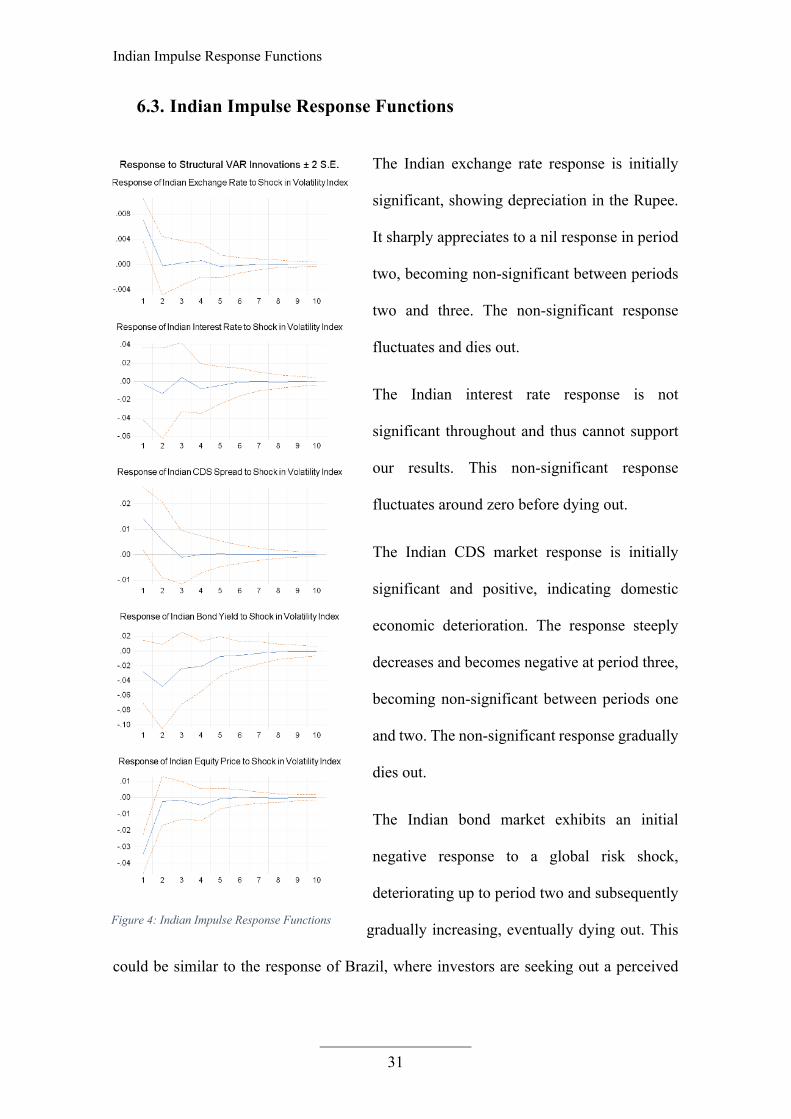
6.3. Indian Impulse Response Functions

The Indian exchange rate response is initially

significant, showing depreciation in the Rupee.

It sharply appreciates to a nil response in period

two, becoming non-significant between periods

two and three. The non-significant response

fluctuates and dies out.

The Indian interest rate response is not

significant throughout and thus cannot support

our results. This non-significant response

fluctuates around zero before dying out.

The Indian CDS market response is initially

significant and positive, indicating domestic

economic deterioration. The response steeply

decreases and becomes negative at period three,

becoming non-significant between periods one

and two. The non-significant response gradually

dies out.

The Indian bond market exhibits an initial

negative response to a global risk shock,

deteriorating up to period two and subsequently

gradually increasing, eventually dying out. This

could be similar to the response of Brazil, where investors are seeking out a perceived

Figure 4: Indian Impulse Response Functions

Indian Impulse Response Functions

___________________

32

safe haven for their investments. The responses, however, are not statistically significant

and thus cannot be considered in our analysis.

The equity market exhibits an initial significant negative response to a global risk shock.

This increases steeply to almost zero at period two, with a negative fluctuation around

period four, eventually dying out. The response becomes non-significant between periods

one and two.

The analysis above indicates a negative economic response to a global risk shock, with

the equity market indicating a significant negative response. The Rupee depreciation and

increase in CDS spreads further indicates economic decline. The responses of interest

rates and bond yields are, however, not statistically significant and thus cannot support

our results.

Chinese Impulse Response Functions

___________________

33

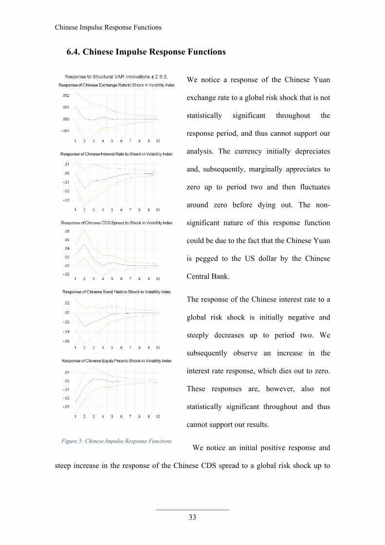
6.4. Chinese Impulse Response Functions

We notice a response of the Chinese Yuan

exchange rate to a global risk shock that is not

statistically significant throughout the

response period, and thus cannot support our

analysis. The currency initially depreciates

and, subsequently, marginally appreciates to

zero up to period two and then fluctuates

around zero before dying out. The non-

significant nature of this response function

could be due to the fact that the Chinese Yuan

is pegged to the US dollar by the Chinese

Central Bank.

The response of the Chinese interest rate to a

global risk shock is initially negative and

steeply decreases up to period two. We

subsequently observe an increase in the

interest rate response, which dies out to zero.

These responses are, however, also not

statistically significant throughout and thus

cannot support our results.

We notice an initial positive response and

steep increase in the response of the Chinese CDS spread to a global risk shock up to

Figure 5: Chinese Impulse Response Functions

Chinese Impulse Response Functions

___________________

34

period two, indicating unfavourable domestic conditions. The response becomes non-

significant between periods two and three, decreasing to zero at period four. This non-

significant response increases marginally at period five and then dies out.

The response of Chinese government bond yields is initially almost nil and decreases

steeply up to period two, again indicating a possible investment safe haven. The bond

yield response begins to increase gradually from period three, eventually dying out. This

response function is also not statistically significant throughout and thus cannot support

our analysis.

The Chinese equity market response to a global risk shock is initially negative and

significant. This gradually increases, becoming positive at period three, after which it

gradually dies out. The response becomes non-significant after period two.

The overall response of the Chinese markets indicates a negative response to the global

risk shock through significant, unfavourable CDS market and equity market responses.

The response of the bond yield, interest rate and exchange rate are, however, not

statistically significant and thus cannot support our findings.

South African Impulse Response Function

___________________

35

6.5. South African Impulse Response Function

The response of the Rand to a global risk shock

is an initial, significant depreciation. The

response decreases sharply up to period two and

gradually dies out. The response becomes non-

significant between periods one and two, and

continues as such.

The initial response of the South African

interest rate is positive and steeply increases

until period two, after which it declines sharply

to period three and gradually dies out. This

response is, however, not statistically

significant throughout, and thus cannot support

our analysis.

We observe an initial positive response to the

global risk shock in the South African CDS

market, again indicating a deterioration in

financial conditions. The error bands indicate

that this response may not be statistically

significant, appearing to extend marginally

below the x-axis. This, however, quickly

corrects with a steep increase up to period two, indicating statistical significance in the

Figure 6: South African Impulse Response Functions

South African Impulse Response Function

___________________

36

CDS spread increase. The response then steeply declines, becoming non-significant

around period three, and gradually dies out.

The response of the South African government bond yield is initially almost zero. This is

followed by a steep decrease to a negative response in period two, which could be

explained through the aforementioned safe haven argument. The yield response

subsequently increases steeply for a period before gradually dying out. This impulse

response function is, however, not statistically significant throughout, and thus cannot be

considered in our results.

The South African equity market exhibits a significant, negative initial response to the

global risk shock. Subsequently, the equity price steeply increases up to period three and

gradually dies out. The response becomes non-significant between periods one and two

and continues as such.

We thus observe the expected negative economic and financial reactions in the South

African market to a deterioration in global risk sentiment with significant currency

depreciation, CDS spread increases and equity price drops. The bond market response as

well as the interest rate response are, again, not statistically significant and thus cannot

be considered in our results.

Initial Impulse Responses

___________________

37

6.6. Initial Impulse Responses

A further means of analysing the

response of each variables to a global

risk shock is to consider the

immediate (i.e. period one) response

of each of the variables to the shock.

We present this in column chart

format grouped both by country as

well as by type of variable, for ease

of comparison.

We observe that, following a global

risk shock, the Russian and Brazilian

markets face the most pressure,

identifiable by the greater magnitude

of initial responses in

macroeconomic and financial variables. We notice fairly consistent responses across the

BRICS in exchange rates and equity prices. The discrepancy in exchange rate responses

with China’s essentially zero result could be due to the Chinese Yuan being pegged to the

US Dollar by the Chinese Central Bank. We further notice a difference in the magnitude

of initial responses of the significant impulse responses, with CDS spreads and equity

market responses appearing to be greater than interest rate responses.

We observe discrepancies in the interest rate responses as well as the government bond

yield responses. The discrepancies in interest rate responses are likely due to interest rates

-0,1

-0,05

0

0,05

0,1

0,15

0,2

Brazil Russia India China South Africa

Initail Response by Country

Exchange Interest CDS Bond Equity

-0,1

-0,05

0

0,05

0,1

0,15

0,2

Exchange Interest CDS Bond Equity

Initial Response per Variable Type

Brazil Russia India China South Africa

Figure 7: Initial Impulse Response by Country

Figure 8: Initial Impulse Response by Variable Type

Initial Impulse Responses

___________________

38

serving as a monetary policy tool of central banks in domestic economies and are thus

artificially manipulated to attain monetary policy objectives. The manually adjusted

nature of these rates results in a delay in response to global financial occurrences, and in

a level of measuring responses to maintain policy objectives and rational expectations

within domestic economies. We cannot rely on these results, however, as they are not

significantly different to zero at the 95% confidence level.

The response discrepancies in government bond yields are likely due to the behavioural

differences in the various BRICS. The initial response of Russian bonds to a global risk

shock is expected, though highly significant, resulting in increased yields and thus a

decrease in the price of government bonds. This is indicative of the deteriorating

economic conditions in Russia. A similar response is observed by the response of South

African government bond yields; however, this response is considered non-significant.

The initial response of Brazil, India and China is a decline in government bond yields,

which indicates an increase in bond prices. This response would generally be considered

unexpected, but may be rationalised, as mentioned earlier, by investors in these countries

seeking stable investments with guaranteed returns, thus opting for these government

bonds due to their highly stable nature. The response of Chinese bonds is, however,

negligible. Again, we cannot reliably utilise the results for Brazil, India, China and South

Africa to support our findings as they are not statistically significant at the 95%

confidence level.

Summative Results

___________________

39

6.7. Summative Results

It is apparent from the data and our analysis that the immediate effect of a global risk

shock on the BRICS economies varies by variable in terms of magnitude and significance.

The effects also vary greatly by country in terms of CDS spreads and government bond

yields.

A global financial risk shock is observed to have a statistically significant effect on all

five BRICS economies in terms of exchange rates (with the exception of the pegged

Chinese Yuan), CDS spreads and equity prices. We notice a positive effect on exchange

rates, signifying a currency depreciation in each country following a risk shock. The effect

on CDS spreads is also positive for all countries, indicating that a risk shock results in a

Figure 9: All Impulse Response Functions to Global Risk Shock

Summative Results

___________________

40

decline in domestic market conditions in each country. Finally, we observe a negative

effect on equity prices following a global risk shock in each country, indicating a

deterioration in domestic equity markets. The statistical significance of the impulse

responses of all three of these variables due to a global risk shock indicates the

deterioration of each domestic economy being linked to a decline in global risk sentiment

and is thus indicative of the spread of contagion effects from developed economies to the

BRICS.

The responses of the interest rates and bond yields across the BRICS, as discussed

previously, contain discrepancies and are thus difficult to interpret reliably without

conjecture. These results, however, are not statistically significant, as indicated by the

error bands in our impulse response functions. We therefore cannot reliably utilise these

responses in our interpretation of results. The clear exception to this non-significance,

however, is that of Russian government bond yields which illustrate a significant positive

response in the bond yields. This is consistent with our theoretical expectations, with a

global risk shock resulting in deteriorated market conditions and thus an increase in bond

yields and a decrease in bond prices. This exception further supports our result of the

spread of contagion effects from developed economies to those of the BRICS.

Model Robustness Analysis

___________________

41

6.8. Model Robustness Analysis

The objective of this section is to assess the SVAR model in terms of robustness. We aim

to determine whether changes to the model will affect the results analysed previously;

namely, global risk shocks exerting a significant effect on exchange rates, CDS spreads

and equity prices in each of the BRICS (besides exchange rates in China), while the

effects on interest rates and bond yields in each of the BRICS is not seen to be statistically

significant (with the exception of bond yield responses in Russia being significant). We

also aim to assess whether the magnitude of these responses is affected by country and

variable.

The factors that we will alter in the model, ceteris paribus, in an effort to investigate its

robustness are the sample period, the measure of global risk, and the identification

scheme. The results of these robustness checks are detailed below.

Robustness Analysis: Sample Period

___________________

42

6.9. Robustness Analysis: Sample Period

In an effort to assess the robustness of our model over time, we alter the sample period of

the data, ceteris paribus, before estimating the model. We utilise a sample period of

January 2002 to December 2019 for this test and analyse the impulse response functions

for this period.

The impulse response functions indicate that our findings remain relatively unchanged

with extremely similar responses in each function to a global risk shock, as well as the

same result of statistical significance and non-significance in every case, as the results of

the original time period analysed. From these results, we conclude that the model is robust

Figure 10: Impulse Response Functions to Robustness Test of Alteration of Sample Period

Robustness Analysis: Measure of Global Risk

___________________

43

in relation to changes in the sample period, with very similar responses being exhibited

over the extended period.

6.10. Robustness Analysis: Measure of Global Risk

In this analysis, the measure of global risk is altered, ceteris paribus, in an effort to gauge

the robustness of the model. We utilise the US Baa corporate spread as the proxy of global

risk appetite as opposed to the Volatility Index, similarly to Yildirim (2016), and analyse

the resulting impulse response functions.

Figure 11: Impulse Response Functions to Robustness Test of Alteration of Global Risk Measure

Robustness Analysis: Identification Scheme

___________________

44

We observe fairly similar response functions to those resulting from the original analysis.

The major differences noted are, firstly, the non-significance of the Indian CDS spread

and Russian bond yield response functions, as well as the shape of the Russian bond yield

response function. This suggests that the negative effects observed in the BRICS

economies are fairly similar, regardless of the global risk measure utilised in the model,

indicating relative robustness in the model.

6.11. Robustness Analysis: Identification Scheme

In the estimation of the SVAR model, an objective was to allow for block exogeneity in

the global risk measure (as well as the US Federal Fund Rate, proxying US monetary

policy). We thus aimed to allow for contemporaneous effects across our domestic

Figure 12: Impulse Response Functions to Robustness Test of Alteration of Identification Scheme

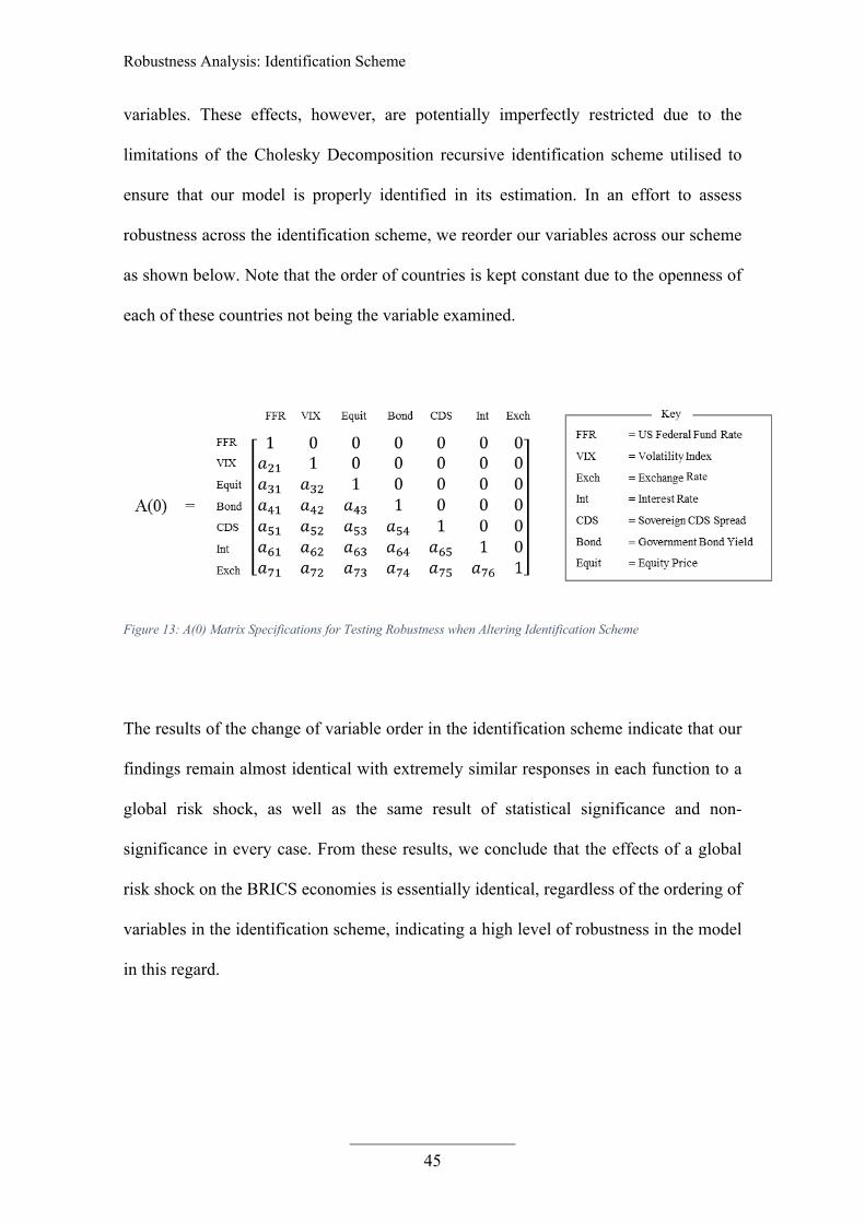
Robustness Analysis: Identification Scheme

___________________

45

variables. These effects, however, are potentially imperfectly restricted due to the

limitations of the Cholesky Decomposition recursive identification scheme utilised to

ensure that our model is properly identified in its estimation. In an effort to assess

robustness across the identification scheme, we reorder our variables across our scheme

as shown below. Note that the order of countries is kept constant due to the openness of

each of these countries not being the variable examined.

Figure 13: A(0) Matrix Specifications for Testing Robustness when Altering Identification Scheme

The results of the change of variable order in the identification scheme indicate that our

findings remain almost identical with extremely similar responses in each function to a

global risk shock, as well as the same result of statistical significance and non-

significance in every case. From these results, we conclude that the effects of a global

risk shock on the BRICS economies is essentially identical, regardless of the ordering of

variables in the identification scheme, indicating a high level of robustness in the model

in this regard.

Rate

Conclusion

___________________

46

7. Conclusion

In this study, we aimed to identify whether contagion effects exist by identifying the

spread of financial shocks from the global economy to the BRICS economies. This was

attempted by implementing a structural vector autoregressive model with block

exogeneity. A number of variables were utilised to model our SVAR. In terms of the

domestic BRICS markets, the macroeconomic factors used were exchange rates and

interest rates and the financial indicators that were utilised were sovereign CDS spreads,

government bond yields and the prices of each country’s primary equity index. The

Volatility Index and the US Federal Fund Rate were utilised as proxies for global factors

in the main analysis.

We investigated a sample period consisting of monthly data from January 2005 to

December 2018. In order to render a reliable, ‘just identified’ SVAR, the block

exogeneity assumption was implemented using the Cholesky Decomposition recursive

identification scheme with the ordering of variables carefully considered. Once the SVAR

had been estimated, impulse response functions were simulated, and bootstrapped by 95%

confidence intervals generated by utilising a Monte Carlo simulation with 250 repetitions.

Through our investigation, we conclude that global risk shocks induce statistically

significant impulse responses in the exchange rates, sovereign CDS spreads and the

equity prices in all the BRICS, with the exception of China’s pegged exchange rate.

Additionally, we further observe a significant response in Russia’s bond market.

However, we cannot draw conclusions from the impulse response functions of the BRICS

countries’ interest rates and the government bond yields (barring Russia) as these

responses to a global risk shock appear to not be statistically significant from zero. The

___________________

47

non-significance of the interest rate responses may be due to the fact that interest rates

serve as a monetary policy tool which is artificially manipulated by central banks, the

revision of which is generally prone to significant lags. As such, we may not use the

results of these impulse response functions to support our conclusion.

We can thus conclude from our analysis that the statistical significance of the impulse

responses to a global risk shock of exchange rates, CDS spreads and equity prices in each

of the BRICS (except exchange rates in China), as well as bond yields in Russia, indicates

the deterioration of each of these domestic economies. This is in line with theoretical

economic predictions, being linked to a decline in global risk sentiment, and is thus

indicative of the spread of contagion effects from the developed global economies to the

BRICS.

The robustness checks of the SVAR model in terms of sample period, global risk measure

and identification scheme indicate a high level of robustness in the estimated model,

which further supports our conclusion of the existence of contagion effects from the

global economy to the BRICS economies.

Recommendations for Further Study

___________________

48

8. Recommendations for Further Study

Through this study and the investigation that led to our final conclusion, we propose

several recommendations that could be proposed for further study on this topic.

We begin with yjr data considerations and limitations identified in this study. Firstly, we

would suggest conducting this research with data of a daily frequency, as daily data are

generally considered to contain more information than monthly data. This may potentially

increase the accuracy and reliability of the estimated model. It must be noted, however,

that this increase in data frequency would likely require software and hardware of greater

processing capacity than EViews 11 and the consumer specification machine utilised in

this study, due to the sheer volume of data observations that would need to be processed.

Secondly, we recommend utilising the industrial production index data as a further

macroeconomic variable pertinent to the domestic economies in the SVAR model. As

mentioned, complete data sets could not be obtained for the purposes of this study,

somewhat limiting our analysis from a macroeconomic variable perspective.

The next consideration we address is that of the limitations in the identification scheme

of our model due to the limited functionality of EViews 11. Due to the limitations found

in the utilisation of EViews 11 as our primary analytical tool, we were bound to the

restrictions placed on the parameters of our A(0) matrix to ensure appropriate

identification of the SVAR, and thus utilised the Cholesky Decomposition as a somewhat

effective, though imperfect solution. We recommend, in further study, the use of more

robust statistical software, such as RATS, in the estimation of the SVAR. Such software

would allow for estimation of far more complex Bayesian VARs, permitting freedom of

restrictions placed on the A(0) matrix parameters and thus providing a means to allow the

___________________

49

modelling of all contemporaneous relationships suggested by economic and financial

theory.

Our final recommendation would be, along with the software recommendations already

proposed, the ability to dynamically adjust parameter restrictions, in order to analyse the

impulse responses of shocks in individual domestic markets variables on the other

remaining BRICS markets, as well as on the measure of global risk. This would allow us

to assess whether these shocks are unidirectional or whether emerging market shocks do

affect the economies of other emerging markets, as well as the global market, thus

purporting the existence of multidirectional contagion.

References

___________________

50

9. References

Allen, F. & Babus, A. (2008) Networks in Finance. Wharton Financial Institutions Center

Working Paper No. 08-07.

Baldwin, R. & Giavazzi, F. (2015). The Eurozone Crisis. A Consensus View of the

Causes and a Few Possible Solutions. London, UK: Centre for Economic Policy

Research Press.

Bekaert, G., Ehrmann, M., Fratzscher M. & Mehl, A. (2014). The Global Crisis and

Equity Market Contagion. The Journal of Finance, 69(6), 2597-2649.

Bonga-Bonga, L. (2018). Uncovering equity market contagion among BRICS countries:

An application of the multivariate GARCH model. The Quarterly Review of

Economics and Finance, 67, 33-44.

CBOE. (2020). CBOE VIX. Turn Volatility to Your Advantage. Accessed 14 January

2020, from: http://www.cboe.com/vix

Chan-Lau, J.A., Mathieson, D.J. & Yao, J.Y. (2004). Extreme Contagion in Equity

Markets. IMF Staff Papers 51(2), 386-408.

Corwin, S.A. & Coughenour, J.F. (2008). Limited Attention and the Allocation of Effort

in Securities Trading. The Journal of Finance, 63(6), 3031-3067.

Cover Design Vectors. [JPEG]. Freepik. Retrieved 10 March 2020, from:

http://www.freepik.com/

References

___________________

51

Dungey, M. & Gajurel, D. (2014). Equity market contagion during the global financial

crisis: Evidence from the world’s eight largest economies. Economic Systems,

38(2), 161-177.

Elliott, M., Golub, B. & Jackson, M. O. (2014). Financial Networks and Contagion. The

American Economic Review, 104(10), 3115-3153.

Forbes, K. & Rigobon, R. (2001). Measuring Contagion: Conceptual and Empirical

Issues. In: Claessens, S. & Forbes, K.J. (Ed.), International Financial Contagion,

43-66. Boston, MA: Springer.

Frank, N. & Hesse, H. (2009). Financial Spillovers to Emerging Markets During the

Global Financial Crisis, IMF Working Paper No. WP/09/104.

Glasserman, P. & Young, H.P. (2015). How likely is contagion in financial networks?

Journal of Banking & Finance, 50(C), 383-399.

Hall, P. (1988). On Symmetric Bootstrap Confidence Intervals. Journal of the Royal

Statistical Society, B50, 35-45.

Horvath, R. (2008). How Important are Foreign Shocks in Small Open Economy? The

Case of Slovakia. William Davidson Institute Working Paper No. 933.

IMF. (2013). Global Financial Stability Report. Transition Challenges to Stability.

Accessed 15 January 2020, from:

https://www.imf.org/External/Pubs/FT/GFSR/2013/02/

Kudlacek, S. (2008). The Interest Rate and Related Macro Economic Variables, Notes.

Analysis of the government bond market and monetary policy. Akelius

References

___________________

52

University. Retrieved 13 January 2020, from:

https://university.akelius.com/library/pdf/the_intere_kudlacek_s0904.pdf

Leitner, Y. (2005). Financial Networks: Contagion, Commitment, and Private-Sector

Bailouts. The Journal of Finance, 60(6), 2925-2953.

Mondria, J. & Quintana-Domeque, C. (2006). Financial Contagion Through Attention

Reallocation: An Empirical Analysis. SSRN. Available online at:

https://ssrn.com/abstract=957185

Mondria, J. & Quintana-Domeque, C. (2013). Financial Contagion and Attention

Allocation. The Economic Journal, 123(568), 429-454.

Nishat, M. & Ullah, W. (2017). Analysis of the government bond market and monetary

policy. International Growth Centre. Accessed 15 January 2020, from:

https://www.theigc.org/project/analysis-of-the-government-bond-market-and-

monetary-policy/

Ozcelebi, O. (2018). Impacts of Exchange Rate Volatility on Macroeconomic and

Financial Variables: Empirical Evidence from PVAR Modelling. IntechOpen.

Retrieved 7 January 2020, from: https://www.intechopen.com/books/trade-and-

global-market/impacts-of-exchange-rate-volatility-on-macroeconomic-and-

financial-variables-empirical-evidence-from

Pesaran, M. H. & Pick, A. (2004). Econometric Issues in the Analysis of Contagion.

CESifo Working Paper No. 1176.

Prabha, A.P., Barth, J.R. & Kim, H. (2009). Spillover Effects from the U.S. Financial

Crisis: Some Time-Series Evidence from National Stock Returns. In: Gup, B.

References

___________________

53

(Ed.), THE FINANCIAL AND ECONOMIC CRISES: AN INTERNATIONAL

PERSPECTIVE. Cheltenham, UK: Edward Elgar Publishing.

Pratama, I., Permanasari, A., Ardiyanto, I. & Indrayani, R. (2016). A review of missing

values handling methods on time-series data. 2016 International Conference on

Information Technology Systems and Innovation (ICITSI). Accessed 16 January

2020, from:

https://www.researchgate.net/publication/313867740_A_review_of_missing_val

ues_handling_methods_on_time-series_data

Roukny, T., Bersini, H., Pirotte, H., Caldarelli, G. & Battiston, S. (2013). Default

Cascades in Complex Networks: Topology and Systemic Risk. Scientific Reports,

3(2759) doi:10.1013/srep02759.

Stiglitz, J.E. (2010). Risk and Global Economic Architecture: Why Full Financial

Integration may be Undesirable. National Bureau of Economic Research Working

Paper No. 15718.

Summer, M. (2013). Financial Contagion and Network Analysis. Annual Review of

Financial Economics, 5(1), 277-297.

Tabarraei. H. (2014). Euro-Crisis and Spillover Effects on the Emerging Economies. Paris

School of Economics Working Paper No. 2014-07.

Tedeschi G., Mazloumian A., Gallegati M. & Helbing D. (2012). Bankruptcy Cascades

in Interbank Markets. PLOS ONE 7(12):e52749.

doi:10.1371/journal.pone.0052749.

References

___________________

54

Viale, A.M., Bessler, D.A. & Kolari, J.W. (2014). Equity market contagion during the

global financial crisis: Evidence from the world’s eight largest economies.

Journal of Applied Economics, 17(2), 373-400.

Yildirim, Z. (2016). Global Financial Conditions and Asset Markets: Evidence from

Fragile Emerging Economies. Economic Modelling, 57(1), 208-220.

Appendix A

___________________

a

Appendix A

Brazil Russia India China South Africa

Interest RateBanco Central Do

Brazil

Federal Reserve Bank of St. Louis -

FRED

Federal Reserve Bank of St. Louis -

FRED

Federal Reserve Bank of St. Louis -

FRED

South African Reserve Bank

Exchange Rate Yahoo! Finance Yahoo! Finance Yahoo! Finance Yahoo! Finance Yahoo! Finance

5 Year Soeverign CDS Spread

Bloomberg Terminal

Bloomberg Terminal

Bloomberg Terminal

Bloomberg Terminal

Bloomberg Terminal

5 Year Government Bond Yield

Federal Reserve Bank of St. Louis -

FRED

Federal Reserve Bank of St. Louis -

FRED

Federal Reserve Bank of St. Louis -

FRED

Federal Reserve Bank of St. Louis -

FRED

Federal Reserve Bank of St. Louis -

FRED

Equity PriceBloomberg Terminal

Bloomberg Terminal

Bloomberg Terminal

Bloomberg Terminal

Bloomberg Terminal

Primary Global Risk Proxy

Volatility Index

US Monetary Policy Proxy

US Federal Fund Rate

Secondary Global Risk Proxy

US BAA Corporate Spread

Chicago Board Options Exchange - VIX Index

Federal Reserve Bank of St. Louis - FRED

Federal Reserve Bank of St. Louis - FRED

Country/Financial Variable

Macroeconomic Variables

Financial Variables

Domestic Block

Global (External)

Block

Table 2: Data Sources