Embed Size (px)
Citation preview
Content-Based Image Retrieval with Relevance
Feedback using Random Walks
Samuel Rota Bulo, Massimo Rabbi and Marcello Pelillo
Dipartimento di Scienze Ambientali, Informatica e Statistica.Universita Ca’ Foscari Venezia
via Torino, 155 - 30172 Mestre-Venezia{srotabul,mrabbi,pelillo}@dsi.unive.it
Abstract
In this paper we propose a novel approach to content-based image retrieval
with relevance feedback, which is based on the random walker algorithm
introduced in the context of interactive image segmentation. The idea is
to treat the relevant and non-relevant images labeled by the user at every
feedback round as “seed” nodes for the random walker problem. The ranking
score for each unlabeled image is computed as the probability that a random
walker starting from that image will reach a relevant seed before encountering
a non-relevant one. Our method is easy to implement, parameter-free and
scales well to large datasets. Extensive experiments on different real datasets
with several image similarity measures show the superiority of our method
over different recent approaches.
Keywords: Random Walks, Content-Based Image Retrieval, Relevance
Feedback
Preprint submitted to Pattern Recognition June 6, 2011

1. Introduction
The concept of relevance feedback, developed during the 1960s to improve
document retrieval processes [1], consists of using user feedback to judge the
relevance of search results and therefore improve their quality through itera-
tive steps. This technique has attracted the Content-Based Image Retrieval
(CBIR) community since the early 1990s and is still an active research topic
nowadays because, in contrast to text/document retrieval, judging the rel-
evance of an image for a user is an almost instantaneous task. Moreover,
by gathering feedbacks from the user a CBIR system can dramatically boost
its performance by reducing the gap between the high-level semantics in the
user’s mind and low-level image descriptors.
Different feedback models have been proposed in the literature (see e.g.,
[2] for a review): positive feedback, which allows the user to select only rele-
vant (positive) images; positive-negative feedback, where the user can specify
both relevant and non-relevant (negative) images; positive-neutral-negative
feedback, where also a neutral class is added among the user’s choices; and
feedback with (non)relevance degree, where the user implicitly ranks the im-
ages by specifying a degree of (non)relevance. The new information inferred
from the user can then be used within a short-term-learning or long-term-
learning process. The former uses the user feedback only within the user’s
query context [3, 4], while the latter updates also the image similarities in
order to benefit from the feedback in future queries [5, 6].
In order to take full advantage of the additional information deriving from
the user interaction, an effective learning method should be adopted in order
to identify relevant and non-relevant images. Moreover, since not all images
2
that have been classified as relevant by the system can be inspected by the
user an implicit ranking of the relevant images is necessary. The approaches
that the literature offers can be divided into inductive and transductive ones
according to whether unlabeled data is used in the training stage or not [7].
The inductive approaches are principally based on Support Vector Machines
(SVM) [8] and boosting [9]. They basically solve a 2-class (relevant and
non-relevant) classification problem and rank the images according to the
classification results. The main disadvantage of these approaches is the low
accuracy caused by the small sample size. Transductive approaches overcome
this problem by exploiting also the information of the unlabeled data. Among
them, we find Manifold-Ranking-Based Image Retrieval (MRBIR) [7], which
propagates a ranking score across the unlabeled data to get the improved
retrieval result, Discriminant-EM [10], which constructs a generative model
by using the unlabeled data to measure the relevance between query and
database images, and Multiple Random Walk (MRW) [11], which creates two
generative models for the two classes of relevant and non-relevant images by
means of Markov random walks. Additionally, in [12] an approach based on
Graph Laplacian is proposed, which allows to learn the embedding of the
manifold enclosing the dataset via diffusion map.
In this paper we propose a novel approach to CBIR with relevance feed-
back, which is inspired by the random walker algorithm for image segmen-
tation introduced by Grady in [13]. Our approach is close in spirit to MR-
BIR and MRW as it casts the CBIR problem with relevance feedback into
a graph-theoretic problem, where nodes are images and image similarities
represent the graph edge weights. The relevant and non-relevant images la-
3

beled by the user at every feedback round are treated as “seed” nodes for
the random walker problem and the ranking score at each unlabeled image is
computed as the probability that a random walker starting from that image
will reach a relevant seed before encountering a non-relevant one along the
graph. Among the positive properties of this formulation we have that the
algorithm is parameter-free, provided that image similarities are given, easy
to implement, and scales well to large datasets as it works also with sparse
graph abstractions of the data. Moreover, although the presented approach
is based on the positive-negative relevance feedback model, it can be eas-
ily adapted to the other models mentioned above. Extensive experiments
on different real datasets with several image similarity measures show the
superiority of our method over different recent approaches.
2. Random Walks for CBIR with Relevance Feedback
The problem of CBIR with relevance feedback can be seen as the problem
of ranking a set of images in a way as to have images visually consistent with
a query image appearing earlier in the ordering. The first K images in
the ranking are presented to the user, who has the opportunity of marking
them as relevant or non-relevant if not satisfied with the result. The user’s
feedback can then be used in order to bridge the semantic-gap between what
he perceives as similar and what the provided low-level similarities classify
as similar.
Since we will model CBIR as a graph-theoretic problem, we start intro-
ducing some basic notions. A graph is a pair G = (V,E), where V is the set
of vertices (nodes) and E ⊆ V ×V is the set of edges, each of which connects
4
two vertices. A weighted graph G = (V,E,w) is a graph with a weight func-
tion w : E → R+, which assigns a nonnegative weight to each edge in the
graph. We will denote by wij the weight associated to edge (i, j) ∈ E. The
(weighted) adjacency matrix of G is given by W = (wij), where we assume
wij = 0 if (i, j) /∈ E, while the (weighted) Laplacian matrix of G is given by
L = D −W , where D = (dij) is a diagonal matrix with dii =∑
j∈V wij.
Consider a CBIR problem, where I = {Ii}Ni=0 is a set of N+1 images, the
first of which is the query image (i.e., I0), and φ is a “low-level” similarity
measure between two images. Each image in I can be seen as a vertex of
an edge-weighted graph G = (V,E,w), where the edges set E consists of
pairs of images for which a weight is defined and the edge-weights reflect the
similarities among images, i.e., wuv = φ(Iu, Iv). The vertex set V corresponds
thus to the index set of I and therefore each image Ij ∈ I is related to a
vertex j ∈ V , vertex 0 representing the query image. In the sequel, we may
refer to the elements of V as images. Beside the graph G, which provides a
static description of the problem, we have to model the information deriving
from the user interaction. We formalize the user, who makes the query and is
involved in the feedback rounds, as a function Ψ : V → {0, 1}, which labels
images, and thus vertices of G, as relevant (1) or non-relevant (0). Note
that Ψ(0) = 1 as the query image I0 is considered relevant for the user. Let
moreover V(r)L ⊆ V , r ≥ 0, be the subset of vertices that have been labeled
by the user within the first r feedback rounds. Note that this set is always
non empty since initially V(0)L = {0}, i.e., it contains the query image. We
will also make the mild assumption that after the first feedback round, i.e.,
for r ≥ 1, at least one non-relevant image appears in V(r)L .
5

Consider now a generic feedback round r > 0. In order to take a decision
about a new ranking of the images based on the user’s feedbacks, our image
retrieval engine requires in input the graph G, the set of labeled vertices
V(r)L collected thus far and the user function Ψ, which provides the label
informations. A new ordering is then produced by assigning a weight x(r)i
to each vertex i ∈ V and by sorting the corresponding images in descending
weight order. We compactly represent all the weights assigned at round r by
a (N + 1)-dimensional column vector x(r) called ranking vector. A property
that the ranking vectors x(r) must satisfy at every round is not to violate the
user’s feedbacks. To this end we impose the following conditions,
(a) 0 ≤ x(r)i ≤ 1, for all i ∈ V ,
(b) x(r)i = Ψ(i), for all i ∈ V (r)
L ,
which guarantee that relevant images will always be top ranked, while non-
relevant ones will always be bottom ranked. Indeed, xi = 1 in the former
case, while xi = 0 in the latter. It is worth noting that we are not interested
in providing a relative ranking of the relevant images, being considered of
equal importance for the user, and therefore they all have the same weight.
Our approach to CBIR with relevance feedback is based on the idea of
interpreting similarities as an indicator of two images to be close within the
ranking. This in terms of the ranking vector means that similar images will
have similar weights, while dissimilar one may have different weights. Ac-
cording to this intuition and keeping conditions (a)-(b) in mind the solution
to our problem at feedback round r can be found by solving the following
6

convex optimization problem:
x(r) = arg minx
∑(i,j)∈E
(xi − xj)2wij ,
subject to conditions (a) and (b).
Note that each term of the energy function encloses the cost of putting two
images apart in the ordering and the higher the similarity of the two images,
the higher this cost will be. Hence, similar images are forced to be close in the
ranking. The constraint set instead guarantees that the ranking vector will
not violate the user feedbacks. Note also that condition (a) can be omitted,
because it is easy to see that all weights are bound in the interval [0, 1].
Therefore, by removing condition (a) and rewriting the energy function in
matrix form our optimization problem becomes simply
x(r) = arg minx
x>Lx ,
subject to xi = Ψ(i) for all i ∈ V (r)L .
(1)
where L is the Laplacian matrix of G. Note that the constraint set can
be completely removed by substituting the fixed components of the ranking
vector in the energy function. This can be easily seen if we opportunely
reorder the vertex set in a way as to have x> = [x>U ,x>M ], where xU is a
vector with the unknown ranking weights of the unlabeled images, while xM
is the vector with the fixed ranking weights of the images marked by the
user. Similarly, the Laplacian matrix L can be block-structured as follows
L =
LUU LUM
LMU LMM
.
7
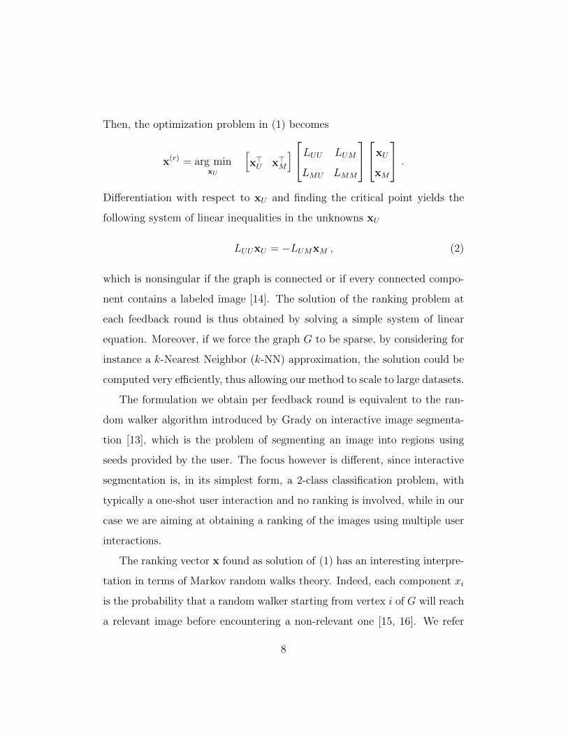
Then, the optimization problem in (1) becomes
x(r) = arg minxU
[x>U x>M
]LUU LUM
LMU LMM
xU
xM
.
Differentiation with respect to xU and finding the critical point yields the
following system of linear inequalities in the unknowns xU
LUUxU = −LUMxM , (2)
which is nonsingular if the graph is connected or if every connected compo-
nent contains a labeled image [14]. The solution of the ranking problem at
each feedback round is thus obtained by solving a simple system of linear
equation. Moreover, if we force the graph G to be sparse, by considering for
instance a k-Nearest Neighbor (k-NN) approximation, the solution could be
computed very efficiently, thus allowing our method to scale to large datasets.
The formulation we obtain per feedback round is equivalent to the ran-
dom walker algorithm introduced by Grady on interactive image segmenta-
tion [13], which is the problem of segmenting an image into regions using
seeds provided by the user. The focus however is different, since interactive
segmentation is, in its simplest form, a 2-class classification problem, with
typically a one-shot user interaction and no ranking is involved, while in our
case we are aiming at obtaining a ranking of the images using multiple user
interactions.
The ranking vector x found as solution of (1) has an interesting interpre-
tation in terms of Markov random walks theory. Indeed, each component xi
is the probability that a random walker starting from vertex i of G will reach
a relevant image before encountering a non-relevant one [15, 16]. We refer
8
to [13] for a description of other connections to discrete potential theory and
the combinatorial Dirichlet problem.
Although the presented theory assumes a positive-negative feedback model,
it is straightforward to generalize it to other models like the positive-neutral-
negative model or the feedback model with relevance degree, by simply re-
placing the user function Ψ. In the positive-neutral-negative case the range of
Ψ would be {0, 0.5, 1}, 0.5 being the score associated to a neutral judgment,
while we may have a continuous interval [0, 1] (or a quantization of it if dis-
crete values are preferred) for models where the user may specify a relevance
degree. We may even design a user function, which simulates a “hesitating”
user, who may change his opinion about feedbacks he previously provided by
simply replacing Ψ.
3. The Algorithm
In this section we summarize our CBIR engine with relevance feedback.
The pseudocode of our approach is presented in Algorithm 1. Our method
requires in input the graph G abstracting the CBIR problem, where vertex
0 ∈ V is assumed to be the query image, the user function Ψ, which encodes
the user’s feedbacks, and a scope size K, which represents the number of
images that should be presented to the user at each feedback round.
At lines 1–3 we set up the system by putting the round counter r to zero,
and by initializing the set of labeled images V(0)L to a singleton with the query
image {0}. Since our method requires at least one non-relevant image to be
specified, we can either force the image having the lowest similarity to the
query image to be non-relevant, or we can present to the user the K images
9

Algorithm 1 Random Walker for CBIR with Relevance Feedback.
Require: graph G = (V,E,w), user Ψ, scope size K
1: {Initialization}
2: r ← 0
3: V(0)L ← {0}
4: S ← get the first K closest images to the query image
5: {Present images indexed by S to the user}
6: while user is not satisfied with S do
7: r ← r + 1
8: {rth feedback round}
9: V(r)L ← V
(r−1)L ∪ S
10: x(r) ← compute the solution of (1) using V(r)L and Ψ
11: S ← get K top ranked vertices according to ranking vector x(r)
12: {Present images indexed by S to the user}
13: end while
10

that are the most similar to the query image. At line 4 we opt for the latter
solution, although the former one may work as well, and we store in the
scope S the K images that will be then presented to the user for gathering
his feedback. At line 6 we enter a loop of relevance feedback rounds, which
will be interrupted as soon as the user is satisfied with the result. We assume
implicit user satisfaction if all the images in the scope are considered relevant
by the user, which formally happens when Ψ(i) = 1 for all i ∈ S. From line
7 to 12 we start a new relevance feedback round. Therefore we increment the
round counter and update the set of labeled images with all those in the scope
S. Note that at any moment we can get the user feedback on each image in
VL through the user function Ψ. At line 10 we compute the ranking vector
as the solution of (1), which involves solving the system of linear equations
(2). The K vertices with higher score in the ranking vector are then stored
in the scope S and presented to the user for a new feedback round.
The proposed algorithm is simple and can be easily implemented. More-
over, there is no parameter that should be tuned. Note also that, as previ-
ously pointed out, the per-round complexity of the algorithm is determined
by step (10), which involves solving a (possibly sparse) linear system of N
equations. The complexity of this task is in general O(N3) for a dense Lapla-
cian matrix and O(N2) for a sparse one, if we consider direct solvers. How-
ever, we are not interested in finding an exact solution of (2), but we want
to discover the relative ordering of the components of the solution. There-
fore, iterative methods may become more appealing, because they smoothly
approach a solution and could be stopped before convergence. Additionally,
the ranking vector obtained in a round can be used to initialize the iterative
11

solver in the next one. This allows to reduce the computational complexity
up to an order of magnitude. We note finally that the running time of our
approach can be further boosted by adopting eigenvector precomputation
techniques as described in [17].
4. Related Works
Approaching the CBIR problem from a graph theoretic perspective, which
involves directly or indirectly Markov random walks, has already been done
in the past, but in a different way.
The Manifold-Ranking algorithm (MRBIR) proposed by He et al. [7] uses
the idea of exploring the relationship among all images in the database and
measures the relevance between them and a query image accordingly. This
transductive approach represents the images in the database as the vertices of
a weighted graph. The user’s relevance feedback is used to generate labeled
examples that help in propagating a ranking score for each image. The
MRBIR framework works with the only-positive as well as positive-negative
feedback models.
A further development of MRBIR by the same authors led to the Multi-
ple Random Walks (MRW) approach [11], which is also one of the methods
we compared against in our experiments. The authors’ idea is to use two
Markov random walks to compute the likelihoods for an image to belong
to the relevant/non-relevant class. These likelihoods are estimated from the
stationary distribution of two Markov chains built upon the original graph of
images with an enlarged set of vertices, which include two (positive and neg-
ative) additional absorbing boundaries. These estimations are then refined
12
by adopting an EM-like procedure.
As opposed to our approach, which is parameter-free, MRW depends on
a parameter α, which should be opportunely tuned. Moreover, the EM-like
refinement process requires a number of iterative steps that should be pre-
estimated. Similar parameters can also be found in the previous MRBIR
algorithm.
Finally, in [12] an approach has been proposed which is based on Graph
Laplacian and allows to learn the embedding of the manifold enclosing the
dataset via diffusion map. The solution of the ranking problem derives from
an unconstrained minimization problem, where the cost function is composed
by a Laplacian term governing the diffusion process and a regularization term
aimed at moving the solution towards the user’s preferences. In contrast to
this formulation, our method consists of a constrained minimization problem,
which can be seen as a limit case of the one in [12]. Indeed, the regularizing
term is replaced by constraints, which force the solution not to violate the
user’s feedback.
5. Experiments
We performed extensive experiments on real datasets with different image
similarity measures and compared against four recent algorithms for CBIR
with relevance feedback.
5.1. Experimental Setting
In our experiments we used three different datasets. The first dataset is
the Wang dataset [18], which is a subset of the known Corel dataset con-
sisting of 1000 images grouped into 10 categories (100 images per category).
13
The second dataset is the Oliva Dataset [19], which encompasses 2688 im-
ages divided into 8 categories. The last dataset is a subset of the Caltech-256
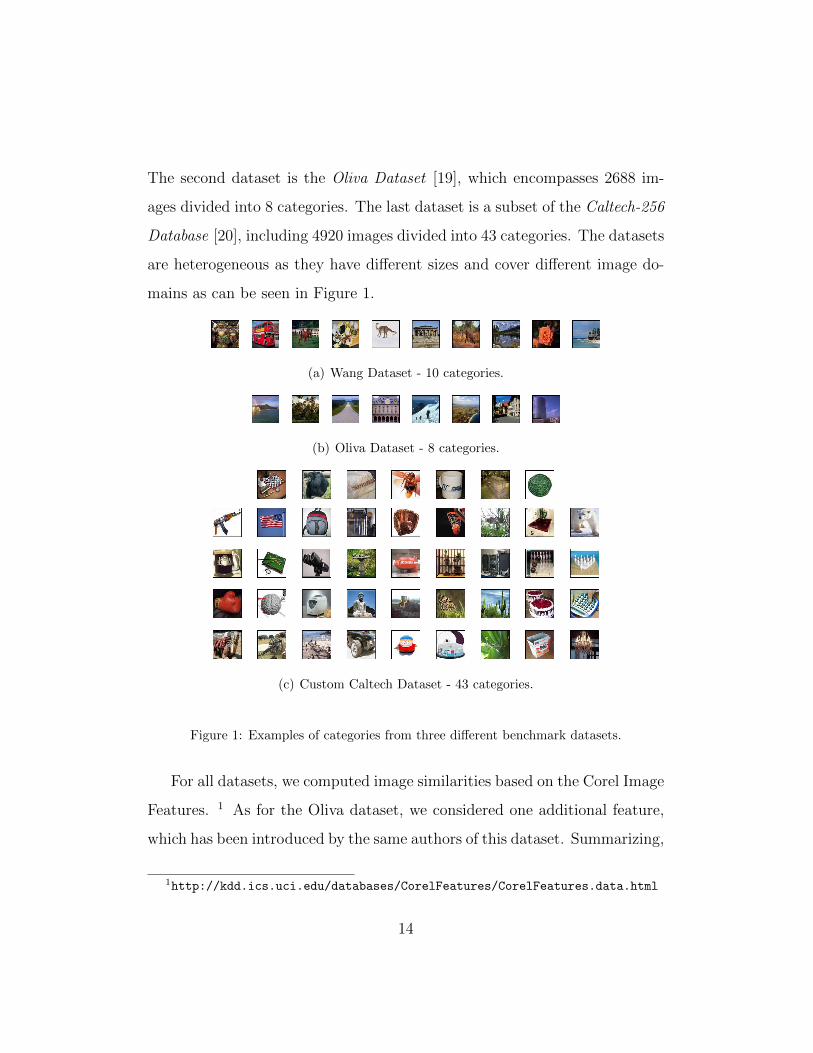
Database [20], including 4920 images divided into 43 categories. The datasets
are heterogeneous as they have different sizes and cover different image do-
mains as can be seen in Figure 1.
(a) Wang Dataset - 10 categories.
(b) Oliva Dataset - 8 categories.
(c) Custom Caltech Dataset - 43 categories.
Figure 1: Examples of categories from three different benchmark datasets.
For all datasets, we computed image similarities based on the Corel Image
Features. 1 As for the Oliva dataset, we considered one additional feature,
which has been introduced by the same authors of this dataset. Summarizing,
1http://kdd.ics.uci.edu/databases/CorelFeatures/CorelFeatures.data.html
14
the following features have been considered in our experiments:
• Color Histogram: the HSV color space is divided into 32 subspaces (32
colors: 8 ranges of H and 4 of S). The density of each color in the image
provides the values for a 32-dimensional feature vector;
• Color Histogram Layout : each image is partitioned into 4 sub-images
and a Color Histogram 4x2 is computed for each sub-image. This yields
a 32-dimensional feature vector (H x S x sub-images = 4 x 2 x 4);
• Color Moments : a 9-dimensional feature vector is computed for each
image by taking the mean, standard deviation and skewness of each
channel of the HSV color space over the image;
• Gray Level Co-Occurrence Matrix : a 20-dimensional feature vector for
each image is computed based on the gray level co-occurrence matrix
(GLCM) [21];
• Global Scene (GIST): a 60-dimensional feature vector is derived from
each image according to Oliva and Torralba’s holistic model, which
tries to represent real-world scenes using a new set of Spatial Envelope
properties [19].
We normalized the feature vectors in a way as to have each component
in the range [0, 1] following [22] and we used `1-norm to compute the dis-
similarity between images. Similarities, where needed, have been computed
using a Gaussian kernel with σ = 1.
We compared our Random Walker (RW) based approach against four
different methods:
15

• Feature Re-Weighting (FR): a method where the importance of the
feature components that best describe the relevant images category is
emphasized [23];
• Relevance Score (RS): a score is computed for each image based on
the distances between the nearest non-relevant image and the nearest
relevant one [24];
• Relevance Score stabilized (RS-S): a variant of the Relevance Score al-
gorithm, which integrates the Bayesian Query Shift framework [25];
• Multiple Random Walk (MRW): for details see Section 4.
In the case of the Wang (1000 images) and Oliva (2688 images) datasets,
we evaluated the performances of the approaches (for each combination of
feature and dataset) over 500 simulated queries, where the query images
have been randomly sampled, while for the Caltech dataset (4920 images)
we reduced the number of queries to 100 due to its large size. We measured
the quality of the results at each feedback round in terms of precision, which
is defined as
precision =n. of relevant retrieved images
scope size
and we computed the average precisions obtained over all the performed
queries in all settings. In our experiments we considered scope sizes of 20,
30 and 40.
At each feedback round, all the unlabeled images within the scope were
automatically labeled using the ground truth in order to simulate the user’s
feedback.
16

5.2. Results
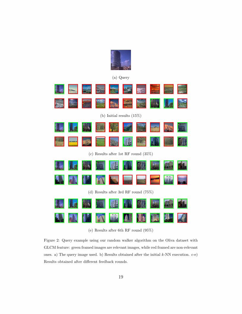
In Figure 2 we provide an example of a query result obtained by our
algorithm on the Oliva dataset with the GLCM feature. We show the results
obtained at different feedback rounds. Green framed images are relevant
ones, while red ones are non-relevant. Our approach performs well despite the
very few relevant images retrieved by the initial k-NN search. The precision
goes up to 65% at the 3th round of relevance feedback and reaches 95% at
the 6th round. It is worth noting that although the GLCM feature provides a
poor description of the image, our method is able to improve the performance
within few feedback rounds. In Figures 3-6 we report also the results obtained
on the same query by the other competing approaches.
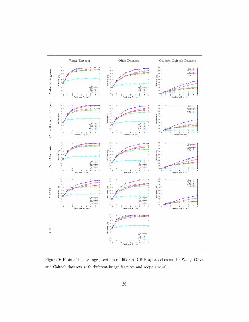
In Figures 7, 8 and 9, we summarize the results obtained in terms of
precision on all datasets, with all the considered features and methods with
scope sizes 20, 30 and 40, respectively. It is evident from an inspection of
all the plots that for all combinations of datasets, features and scope sizes
our method outperforms the competitors. On the other hand, the Feature
Re-Weighting approach turns out to be the worst method in all tests. We
also notice that it exhibits a stationary behavior after the third or fourth
round of relevance feedback.
The overall results are better, as one could expect, on datasets with nar-
row image domains and less categories, like in the case of the Wang dataset,
as opposed to larger ones like the Caltech dataset. Indeed, our algorithm,
which achieves the best results, never exceeds 60% of precision. Moreover,
the performances are definitely affected by the choice of the image features
used to describe the whole image. This can be noticed in particular in the
17
Oliva dataset, where the GIST features allow our approach to obtain very
high precision scores after few feedback rounds.
From a global perspective, it becomes apparent that approaches to CBIR
with relevance feedback based on random walks are promising. Indeed, the
MRW approach is in many cases the second best performing approach.
5.3. Running Time
In the experiments presented in the previous subsection, we worked with
dense graphs. We run the experiments with MatLab on a machine equipped
with 8 Intel Xeon 2.33 GHz CPUs and 8 GB RAM. In Figure 10 we report the
average running time per round registered by each approach on the different
datasets with the Color Histogram feature. Our RW method outperforms re-
markably the other random-walk-based approach M-RW on all the datasets.
Specifically, on the largest datasets (Oliva and Caltech) our algorithm yields
higher running time compared to FR, RS, RS-S. However, this speed differ-
ence is justified by a significantly higher precision as shown in the previous
section. On the Wang dataset, instead, our algorithm is competitive also in
terms of running time. Note that in Figure 10 we do not report the results
obtained for each feature, since the influence of the feature adopted on the
running time is on average irrelevant.
A distinct feature of our approach, and in general of random-walk-based
ones, is that it works even if we render the graph G sparse. This allows
us to considerably reduce the time needed to compute the ranking vector.
We performed preliminary experiments in order to test the gains in terms
of running time and the influence that the graph approximation has on the
precision of our RW approach. Specifically, we run experiments on the Oliva
18
(a) Query
(b) Initial results (15%)
(c) Results after 1st RF round (35%)
(d) Results after 3rd RF round (75%)
(e) Results after 6th RF round (95%)
Figure 2: Query example using our random walker algorithm on the Oliva dataset with
GLCM feature: green framed images are relevant images, while red framed are non-relevant
ones. a) The query image used. b) Results obtained after the initial k-NN execution. c-e)
Results obtained after different feedback rounds.
19

(a) Query
(b) Initial results (15%)
(c) Results after 1st RF round (10%)
(d) Results after 3rd RF round (10%)
(e) Results after 6th RF round (20%)
Figure 3: Query example using the feature re-weighting algorithm on the Oliva dataset
with GLCM feature: green framed images are relevant images, while red framed are non-
relevant ones. a) The query image used. b) Initial results obtained by the algorithm. c-e)
Results obtained after different feedback rounds.
20

(a) Query
(b) Initial results (15%)
(c) Results after 1st RF round (45%)
(d) Results after 3rd RF round (65%)
(e) Results after 6th RF round (80%)
Figure 4: Query example using the relevance score algorithm on the Oliva dataset with
GLCM feature: green framed images are relevant images, while red framed are non-relevant
ones. a) The query image used. b) Initial results obtained by the algorithm. c-e) Results
obtained after different feedback rounds.
21

(a) Query
(b) Initial results (15%)
(c) Results after 1st RF round (45%)
(d) Results after 3rd RF round (65%)
(e) Results after 6th RF round (80%)
Figure 5: Query example using the relevance score stabilized algorithm on the Oliva
dataset with GLCM feature: green framed images are relevant images, while red framed are
non-relevant ones. a) The query image used. b) Initial results obtained by the algorithm.
c-e) Results obtained after different feedback rounds.
22

(a) Query
(b) Initial results (10%)
(c) Results after 1st RF round (15%)
(d) Results after 3rd RF round (40%)
(e) Results after 6th RF round (80%)
Figure 6: Query example using the multiple random walk algorithm on the Oliva dataset
with GLCM feature: green framed images are relevant images, while red framed are non-
relevant ones. a) The query image used. b) Initial results obtained by the algorithm. c-e)
Results obtained after different feedback rounds.
23

Wang Dataset Oliva Dataset Custom Caltech Dataset
ColorHistogram
10
20
30
40
50
60
70
80
90
100
0 1 2 3 4 5 6 7 8
Pre
cisi
on (
%)
Feedback Rounds
RS RS-S
RW MRW
FR 10
20
30
40
50
60
70
80
90
100
0 1 2 3 4 5 6 7 8
Pre
cisi
on (
%)
Feedback Rounds
RS RS-S
RW MRW
FR 10
20
30
40
50
60
70
80
90
100
0 1 2 3 4 5 6 7 8
Pre
cisi
on (
%)
Feedback Rounds
RS RS-S
RW MRW
FR
ColorHistogram
Layout
10
20
30
40
50
60
70
80
90
100
0 1 2 3 4 5 6 7 8
Pre
cisi
on (
%)
Feedback Rounds
RS RS-S
RW MRW
FR 10
20
30
40
50
60
70
80
90
100
0 1 2 3 4 5 6 7 8
Pre
cisi
on (
%)
Feedback Rounds
RS RS-S
RW MRW
FR 10
20
30
40
50
60
70
80
90
100
0 1 2 3 4 5 6 7 8
Pre
cisi
on (
%)
Feedback Rounds
RS RS-S
RW MRW
FR
ColorMomen
ts
10
20
30
40
50
60
70
80
90
100
0 1 2 3 4 5 6 7 8
Pre
cisi
on (
%)
Feedback Rounds
RS RS-S
RW MRW
FR 10
20
30
40
50
60
70
80
90
100
0 1 2 3 4 5 6 7 8
Pre
cisi
on (
%)
Feedback Rounds
RS RS-S
RW MRW
FR 10
20
30
40
50
60
70
80
90
100
0 1 2 3 4 5 6 7 8
Pre
cisi
on (
%)
Feedback Rounds
RS RS-S
RW MRW
FR
GLCM
10
20
30
40
50
60
70
80
90
100
0 1 2 3 4 5 6 7 8
Pre
cisi
on (
%)
Feedback Rounds
RS RS-S
RW MRW
FR 10
20
30
40
50
60
70
80
90
100
0 1 2 3 4 5 6 7 8
Pre
cisi
on (
%)
Feedback Rounds
RS RS-S
RW MRW
FR 10
20
30
40
50
60
70
80
90
100
0 1 2 3 4 5 6 7 8
Pre
cisi
on (
%)
Feedback Rounds
RS RS-S
RW MRW
FR
GIST
10
20
30
40
50
60
70
80
90
100
0 1 2 3 4 5 6 7 8
Pre
cisi
on (
%)
Feedback Rounds
RS RS-S
RW MRW
FR
Figure 7: Plots of the average precision of different CBIR approaches on the Wang, Oliva
and Caltech datasets with different image features and scope size 20.
24

Wang Dataset Oliva Dataset Custom Caltech Dataset
ColorHistogram
10
20
30
40
50
60
70
80
90
100
0 1 2 3 4 5 6 7 8
Pre
cis
ion
(%
)
Feedback Rounds
RS RS-S
RW MRW
FR 10
20
30
40
50
60
70
80
90
100
0 1 2 3 4 5 6 7 8
Pre
cis
ion
(%
)
Feedback Rounds
RS RS-S
RW MRW
FR 10
20
30
40
50
60
70
80
90
100
0 1 2 3 4 5 6 7 8
Pre
cis
ion
(%
)
Feedback Rounds
RS RS-S
RW MRW
FR
ColorHistogram
Layout
10
20
30
40
50
60
70
80
90
100
0 1 2 3 4 5 6 7 8
Pre
cis
ion
(%
)
Feedback Rounds
RS RS-S
RW MRW
FR 10
20
30
40
50
60
70
80
90
100
0 1 2 3 4 5 6 7 8
Pre
cis
ion
(%
)
Feedback Rounds
RS RS-S
RW MRW
FR 10
20
30
40
50
60
70
80
90
100
0 1 2 3 4 5 6 7 8
Pre
cis
ion
(%
)
Feedback Rounds
RS RS-S
RW MRW
FR
ColorMomen
ts
10
20
30
40
50
60
70
80
90
100
0 1 2 3 4 5 6 7 8
Pre
cis
ion
(%
)
Feedback Rounds
RS RS-S
RW MRW
FR 10
20
30
40
50
60
70
80
90
100
0 1 2 3 4 5 6 7 8
Pre
cis
ion
(%
)
Feedback Rounds
RS RS-S
RW MRW
FR 10
20
30
40
50
60
70
80
90
100
0 1 2 3 4 5 6 7 8
Pre
cis
ion
(%
)
Feedback Rounds
RS RS-S
RW MRW
FR
GLCM
10
20
30
40
50
60
70
80
90
100
0 1 2 3 4 5 6 7 8
Pre
cis
ion
(%
)
Feedback Rounds
RS RS-S
RW MRW
FR 10
20
30
40
50
60
70
80
90
100
0 1 2 3 4 5 6 7 8
Pre
cis
ion
(%
)
Feedback Rounds
RS RS-S
RW MRW
FR 10
20
30
40
50
60
70
80
90
100
0 1 2 3 4 5 6 7 8
Pre
cis
ion
(%
)
Feedback Rounds
RS RS-S
RW MRW
FR
GIST
10
20
30
40
50
60
70
80
90
100
0 1 2 3 4 5 6 7 8
Pre
cis
ion
(%
)
Feedback Rounds
RS RS-S
RW MRW
FR
Figure 8: Plots of the average precision of different CBIR approaches on the Wang, Oliva
and Caltech datasets with different image features and scope size 30.
25
Wang Dataset Oliva Dataset Custom Caltech Dataset
ColorHistogram
10
20
30
40
50
60
70
80
90
100
0 1 2 3 4 5 6 7 8
Pre
cis
ion
(%
)
Feedback Rounds
RS RS-S
RW MRW
FR 10
20
30
40
50
60
70
80
90
100
0 1 2 3 4 5 6 7 8
Pre
cis
ion
(%
)
Feedback Rounds
RS RS-S
RW MRW
FR 10
20
30
40
50
60
70
80
90
100
0 1 2 3 4 5 6 7 8
Pre
cis
ion
(%
)
Feedback Rounds
RS RS-S
RW MRW
FR
ColorHistogram
Layout
10
20
30
40
50
60
70
80
90
100
0 1 2 3 4 5 6 7 8
Pre
cis
ion
(%
)
Feedback Rounds
RS RS-S
RW MRW
FR 10
20
30
40
50
60
70
80
90
100
0 1 2 3 4 5 6 7 8
Pre
cis
ion
(%
)
Feedback Rounds
RS RS-S
RW MRW
FR 10
20
30
40
50
60
70
80
90
100
0 1 2 3 4 5 6 7 8
Pre
cis
ion
(%
)
Feedback Rounds
RS RS-S
RW MRW
FR
ColorMomen
ts
10
20
30
40
50
60
70
80
90
100
0 1 2 3 4 5 6 7 8
Pre
cis
ion
(%
)
Feedback Rounds
RS RS-S
RW MRW
FR 10
20
30
40
50
60
70
80
90
100
0 1 2 3 4 5 6 7 8
Pre
cis
ion
(%
)
Feedback Rounds
RS RS-S
RW MRW
FR 10
20
30
40
50
60
70
80
90
100
0 1 2 3 4 5 6 7 8
Pre
cis
ion
(%
)
Feedback Rounds
RS RS-S
RW MRW
FR
GLCM
10
20
30
40
50
60
70
80
90
100
0 1 2 3 4 5 6 7 8
Pre
cis
ion
(%
)
Feedback Rounds
RS RS-S
RW MRW
FR 10
20
30
40
50
60
70
80
90
100
0 1 2 3 4 5 6 7 8
Pre
cis
ion
(%
)
Feedback Rounds
RS RS-S
RW MRW
FR 10
20
30
40
50
60
70
80
90
100
0 1 2 3 4 5 6 7 8
Pre
cis
ion
(%
)
Feedback Rounds
RS RS-S
RW MRW
FR
GIST
10
20
30
40
50
60
70
80
90
100
0 1 2 3 4 5 6 7 8
Pre
cis
ion
(%
)
Feedback Rounds
RS RS-S
RW MRW
FR
Figure 9: Plots of the average precision of different CBIR approaches on the Wang, Oliva
and Caltech datasets with different image features and scope size 40.
26

1e-05
0.0001
0.001
0.01
0.1
1
10
0 1 2 3 4 5 6 7 8
Ave
rage
tim
e pe
r ro
und
Feedback Rounds
RS RS-S
RW MRW
FR
(a) Wang dataset
1e-05
0.0001
0.001
0.01
0.1
1
10
100
0 1 2 3 4 5 6 7 8
Ave
rage
tim
e pe
r ro
und
Feedback Rounds
RS RS-S
RW MRW
FR
(b) Oliva dataset
0.001
0.01
0.1
1
10
100
1000
0 1 2 3 4 5 6 7 8
Ave
rage
tim
e pe
r ro
und
Feedback Rounds
RS RS-S
RW MRW
FR
(c) Caltech dataset
Figure 10: Average running time per round for the Wang, Oliva and Caltech datasets with
the Color Histogram feature.
dataset, by considering all features, using a k-NN graph approximation with
k = 20. Figure 11 reports the results. Surprisingly, by using the sparse graph
we registered an overall increase in the average precision of our approach, and
a considerable reduction of the average running time.
5.4. Conclusions
In this paper we proposed a novel approach to CBIR with relevance feed-
back, which is based on the random walker algorithm introduced in the con-
text of interactive image segmentation. Relevant and non-relevant images
labeled by the user at every feedback round are used as “seed” nodes for the
random walker problem. Each unlabeled image is finally ranked according
to the probability that a random walker starting from that image will reach
a relevant seed before encountering a non-relevant one. Our method is easy
to implement, it has no parameters to tune and scales well to large datasets.
Extensive experiments on different real datasets with several image similarity
measures have shown the superiority of the proposed method over different
recent approaches.
27

Precision Running time
ColorHistogram
10
20
30
40
50
60
70
80
90
100
0 1 2 3 4 5 6 7 8
Pre
cisi
on (
%)
Feedback Rounds
Original G Sparse G
0.001
0.01
0.1
1
10
0 1 2 3 4 5 6 7 8
Ave
rage
tim
e pe
r ro
und
Feedback Rounds
Original G Sparse G
ColorHistogram
Layout
10
20
30
40
50
60
70
80
90
100
0 1 2 3 4 5 6 7 8
Pre
cisi
on (
%)
Feedback Rounds
Original G Sparse G
0.001
0.01
0.1
1
0 1 2 3 4 5 6 7 8
Ave
rage
tim
e pe
r ro
und
Feedback Rounds
Original G Sparse G
ColorMomen
ts
10
20
30
40
50
60
70
80
90
100
0 1 2 3 4 5 6 7 8
Pre
cisi
on (
%)
Feedback Rounds
Original G Sparse G
0.001
0.01
0.1
1
0 1 2 3 4 5 6 7 8
Ave
rage
tim
e pe
r ro
und
Feedback Rounds
Original G Sparse G
GLCM
10
20
30
40
50
60
70
80
90
100
0 1 2 3 4 5 6 7 8
Pre
cisi
on (
%)
Feedback Rounds
Original G Sparse G
0.001
0.01
0.1
1
0 1 2 3 4 5 6 7 8
Ave
rage
tim
e pe
r ro
und
Feedback Rounds
Original G Sparse G
GIST
10
20
30
40
50
60
70
80
90
100
0 1 2 3 4 5 6 7 8
Pre
cisi
on (
%)
Feedback Rounds
Original G Sparse G
1e-05
0.0001
0.001
0.01
0.1
1
0 1 2 3 4 5 6 7 8
Ave
rage
tim
e pe
r ro
und
Feedback Rounds
Original G Sparse G
Figure 11: Comparison of the RW performance on the Oliva dataset with all features in the
cases when a dense and sparse graph G is used. The sparse graph is a k-NN approximation
of the original graph G, where k = 20.
28

References
[1] J. J. Rocchio, Document retrieval systems - optimization and evaluation,
Ph.D. thesis, Harvard Computational Laboratory, Harvard University,
Cambridge, 1966.
[2] X. S. Zhou, T. S. Huang, Relevance feedback for image retrieval: A
comprenhensive review, Multim. Systems 8 (6) (2003) 536–544.
[3] Y. Rui, T. S. Huang, M. Ortega, S. Mehrotra, Relevance feedback: A
power tool for interactive content-based image retrieval, IEEE Trans.
Circuits and Syst. for Video and Techn. 8 (5) (1998) 644–655.
[4] A. Kushki, P. Androutsos, K. N. Plataniotis, A. N. Venetsanopoulos,
Query feedback for interactive image retrieval, IEEE Trans. Circuits
and Syst. for Video and Techn. 14 (5) (2004) 644–655.
[5] J. Fournier, M. Cord, Long-term similarity learning in content-based
image retrieval., in: Int. Conf. Image Processing (ICIP), 441–444, 2002.
[6] M. Cord, P. H. Gosselin, Image Retrieval using Long-Term Semantic
Learning, in: Int. Conf. Image Processing (ICIP), 2909–2912, 2006.
[7] J. He, M. Li, H. Zhang, H. Tong, C. Zhang, Manifold-ranking based
image retrieval, in: Int. Conf. on Multimedia, 9–16, 2004.
[8] L. Zhang, F. Lin, B. Zhang, Support Vector Machine Learning for Image
Retrieval, in: Int. Conf. Image Processing (ICIP), 721–724, 2001.
[9] K. Tieu, P. Viola, Boosting image retrieval, in: IEEE Conf. Computer
Vision and Patt. Recogn. (CVPR), vol. 1, 228–235, 2000.
29

[10] Y. Wu, Q. Tian, T. Huang, Discriminant-EM algorithm with application
to image retrieval, in: Int. Conf. Image Processing (ICIP), vol. 1, 155–
162, 2000.
[11] J. He, H. Tong, M. Li, W. Y. Ma, C. Zhang, Multiple random walk and
its application in content-based image retrieval, in: Int. Workshop on
Mult. Inf. Retrieval, 151–158, 2005.
[12] H. Sahbi, P. Etyngier, J. Y. Audibert, R. Keriven, Manifold Learning
using Robust Graph Laplacian for Interactive Image Search, in: IEEE
Conf. Computer Vision and Patt. Recogn. (CVPR), 1–8, 2008.
[13] L. Grady, Random walks for image segmentation, IEEE Trans. Pattern
Anal. Machine Intell. 28 (11) (2006) 1768–1783.
[14] E. Mortensen, W. Barrett, Interactive segmentation with intelligent scis-
sors, Graph. Mod. in Image Processing 60 (5) (1998) 349–384.
[15] S. Kakutani, Markov processes and the Dirichlet problem, Proc. Jap.
Acad. 21 (21) (1945) 227–233.
[16] P. Doyle, L. Snell, Random walks and eletric networks, no. 22 in Carus
mathematical monographs, Mathematical Association of America, 1984.
[17] L. Grady, A. K. Sinop, Fast approximate Random Walker segmentation
using eigenvector precomputation, in: IEEE Conf. Computer Vision and
Patt. Recogn. (CVPR), 1–8, 2008.
[18] G. W. J. Z. Wang, J. Li, SIMPLIcity: Semantics-sensitive Integrated
30
Matching for Picture LIbraries, IEEE Trans. Pattern Anal. Machine
Intell. 23 (9) (2001) 947–963.
[19] A. Oliva, A. Torralba, Modeling the Shape of the Scene: A Holistic
Representation of the Spatial Envelope, Int. J. Comput. Vision 42 (3)
(2001) 145–175.
[20] G. Griffin, A. Holub, P. Perona, Caltech-256 object category dataset,
Tech. Rep. 7694, California Institute of Technology, 2007.
[21] R. M. Haralick, K. S. Shanmugan, I. Dunstein, Textural features for
image classification, IEEE Trans. Syst. Man & Cybern. 3 (6) (1973)
610–621.
[22] S. Aksoy, R. M. Haralick, Feature normalization and likelihood-based
similarity measures for image retrieval, Pattern Recogn. Letters 22 (5)
(2001) 563–582.
[23] G. Das, S. Ray, C. Wilson, Feature re-weighting in content-based image
retrieval, in: Int. Conf. in Image and Video Retr., 193–200, 2006.
[24] G. Giacinto, F. Roli, Instance-Based Relevance Feedback for Image Re-
trieval, in: Adv. in Neural Inform. Process. Syst. (NIPS), vol. 17, 489–
496, 2005.
[25] G. Giacinto, A nearest-neighbor approach to relevance feedback in con-
tent based image retrieval, in: Int. Conf. in Image and Video Retr.,
456–463, 2007.
31