EFFECTS OF COMPETITION AMONG INTERNET SERVICE PROVIDERS AND

CONTENT PROVIDERS ON THE NET NEUTRALITY DEBATE

Hong Guo*, Subhajyoti Bandyopadhyay**, Arthur Lim*, Yu-Chen Yang***, Kenny Cheng**

* University of Notre Dame, {hguo, arthurlim}@nd.edu

** University of Florida, {shubho.bandyopadhyay, kenny.cheng}@warrington.ufl.edu

*** National Sun Yat-sen University, ycyang@mis.nsysu.edu.tw

ABSTRACT

Supporters of net neutrality have often argued that more competition among Internet service

providers (ISPs) is beneficial for an open Internet and that the market power of the ISPs lies

at the heart of the net neutrality debate. However, the joint effects of the competition among

ISPs and among content providers have yet to be examined. We study the critical linkage

between ISP competition and content provider competition, as well as its policy implications.

We find that even under competitive pressure from a rival ISP, an ISP still has the incentive

and the ability to enforce charging content providers for priority delivery of content.

Upending the commonly held belief that content providers will always support the

preservation of net neutrality, we find that under certain conditions, it is economically

beneficial for the dominant content provider to reverse its stance on net neutrality. Our paper

also makes an important contribution in extending the traditional two-dimensional

spatial-competition literature.

Keywords: Net Neutrality, Internet Service Provider Competition, Content Provider

Competition, Packet Discrimination, Social Welfare

1

EFFECTS OF COMPETITION AMONG INTERNET SERVICE PROVIDERS AND

CONTENT PROVIDERS ON THE NET NEUTRALITY DEBATE

INTRODUCTION

The Federal Communications Commission (FCC)’s path to enforce net neutrality rules to

preserve an open Internet has been complicated and controversial. In its 2010 Open Internet

Order, the FCC proposed net neutrality rules consisting of four core principles: transparency,

no blocking, no unreasonable discrimination, and reasonable network management (FCC

2010). These rules were later struck down by the U.S. Court of Appeals for the District of

Columbia Circuit, which assessed that the FCC only has limited regulatory options for

broadband as an information service (Nagesh and Sharma 2014). During a five-month period

in 2014, to better inform its new rulemaking, the FCC solicited public comments on net

neutrality issue and received a total of 3.7 million comments, which makes it the most

commented-upon issue in the agency’s history.

The recent FCC decision to adopt new net neutrality rules that would allow

“commercially reasonable” traffic management has been criticized by several proponents of

net neutrality (Snider and Yu 2014; Wyatt 2014). Proponents of net neutrality have long

opined that a lack of effective competition in the local broadband market enables Internet

service providers (ISPs) to act as gatekeepers of content, and thus to be in a position to charge

content providers (CPs) for priority delivery of their data packets1. The appeals court made

the same argument as part of its ruling: “...if end users could immediately respond to any

given broadband provider’s attempt to impose restrictions on edge providers by switching

broadband providers, this gatekeeper power might well disappear... For example, a broadband

provider like Comcast would be unable to threaten Netflix that it would slow Netflix traffic if

1 This paid prioritization is also referred to as packet discrimination. 2

all Comcast subscribers would then immediately switch to a competing broadband provider.”

(U.S. Court of Appeals 2014)

Supporters of net neutrality have often argued that more competition among ISPs is

beneficial for an open Internet (Glaser 2014; Dunbar 2014) and that the market power of the

ISPs lies at the heart of the net neutrality debate (Mcmillan 2014; Winegarden 2014). They

argue that competition among ISPs would prevent them from gaining the market power that

currently allows them to charge consumers supra-competitive prices for Internet access

services and to potentially charge content providers for preferential delivery services. In fact,

there have been several calls to remove the barriers to a competitive broadband market

(Szoka et al. 2013). Net neutrality, however, has not been a major concern for countries with

more competitive ISP markets, such as Australia and South Korea.

In this paper, we investigate whether the presence of competition in local broadband

markets would indeed prevent ISPs from charging online content providers for preferred

delivery. Our analysis builds upon the extant research of Choi and Kim (2010) and Cheng et

al. (2011), who examined the net neutrality issue for a monopoly ISP. The contribution of our

research is to show that even under competitive pressure from a rival ISP, an ISP still has the

incentive and the ability to enforce charging content providers for priority delivery of

content.

The issue of competition among content providers has thus far taken a back seat in the

net neutrality debate. Content providers have been among the strongest proponents of net

neutrality (The Internet Association 2014). Recent developments, however, show some

deviations from this stance. Manjoo (2014) observed that in contrast to the recent grassroots

movements over the ongoing discussions regarding net neutrality regulation, the large

Internet companies “have not joined online protests, or otherwise moved to mobilize their

users in favor of new rules.” Google has been questioned for its stance on net neutrality after

3

its entry into the broadband market through Google Fiber (Singel 2013). Two important

issues remain unaddressed: to wit, how competitive pressures drive content providers to pay

for preferential delivery and how their choices affect the ISPs’ incentives to manage their

traffic.

We investigate the impact of content provider competition in the presence of ISP

competition. One question that is of particular interest is whether sufficient market power of

the content provider encourages it to abandon its support for net neutrality. We find that a

dominating content provider may be better off without net neutrality given sufficient market

power relative to that of the ISPs. We study the critical linkage between ISP competition and

content provider competition, as well as its policy implications. Our findings suggest that the

impact of net neutrality regulation on the incentives of content providers depends critically on

the market power of the competitors both within the local ISP market and within the content

market.

Apart from these policy prescriptions, this paper makes an important contribution in

extending the traditional two-dimensional spatial-competition literature. The proposed model

captures the relevant characteristics of data transmission in the net neutrality debate. More

generally, the modeling framework can be used to analyze the competition between two sets

of firms providing complementary products that are consumed together to constitute the total

end-user experience (e.g. computer hardware platforms and the software on those platforms).

The paper is organized as follows: In the next section, we review the related literature

and discuss the contributions of this paper in that context. We then propose a two-sided

market model of Internet data transmission with both ISP competition and content provider

competition. Following that, we analyze the outcomes under both net neutrality and packet

discrimination regimes, with a focus on the impact of ISP competition and content provider

competition. The paper concludes with theoretical, managerial, and policy implications.

4

LITERATURE REVIEW

In this section, we review the fast-growing literature of economic analysis of net neutrality.

For a broader review of the network neutrality literature see Krämer et al. (2013). Studies in

network interconnection (Armstrong 1998; Laffont et al. 2003; Tan et al. 2006; Chiang and

Jhang-Li 2014) focus on the issues of interconnection settlements among backbone network

providers. The issue of net neutrality, however, focuses on “last-mile” ISPs that provide

Internet access services to their local consumers.

Existing models make different assumptions about the market structure of Internet

data transmission within the last mile and find a variety of results on the key economic

outcomes (such as content innovation and social welfare, etc.) in the net neutrality debate.

Hermalin and Katz (2007) find that net neutrality reduces the set of available content

and thus leads to lower content innovation. Economides and Tåg (2012) conclude that there

are more active content providers under net neutrality, when the value of an additional

consumer to the content providers exceeds the value of an additional content provider to the

consumers. Krämer and Wiewiorra (2012) model congestion-sensitive content providers with

differing congestion-sensitivity distributions and find that content innovation is lower under

net neutrality for less congestion-sensitive content providers, and higher for more

congestion-sensitive content providers. Guo et al. (2012) find that abandoning the principle of

net neutrality can hinder the ability of startups to compete against established rivals and thus

reduce innovation at the edge.

The results are mixed when it comes to evaluating the impact of the potential net

neutrality regulation on social welfare. Some papers (Cheng et al. 2011; Guo et al. 2012;

Krämer and Wiewiorra 2012; Bourreau et al. 2014; Guo and Easley 2014) find that net

neutrality results in lower social welfare compared to packet discrimination, while others

(Hermalin and Katz 2007; Choi and Kim 2010; Economides and Hermalin 2012; Economides

5

and Tåg 2012) obtain mixed welfare results. Most of the articles agree, however, that if

packet discrimination were permitted, the ISP would be better off while content providers

would be worse off, due to the ISP's added flexibility in network management.

From the perspective of modeling ISP competition, most extant models consider a

monopoly ISP, though Hermalin and Katz (2007) and Economides and Tåg (2012) extend

their models to consider the effects of ISP competition and in either case find results similar

to the monopoly case. Bourreau et al. (2014) extend the model proposed in Krämer and

Wiewiorra (2012) to allow ISP competition. They find that the packet discrimination regime

results in higher infrastructure investment, more content innovation, and higher overall social

welfare. The ISPs, however, may be worse off under the packet discrimination regime, due to

intensified competition in the consumer market. Bykowsky and Sharkey (2014) study the

welfare effects of the zero-price rule under various conditions of the ISPs’ market power.

They find that the zero-price rule is welfare enhancing if and only if the ISP’s ability to

establish competitive prices for the content providers exceeds its ability to establish such

prices for consumers.

From the perspective of modeling content provider competition, most authors assume

that content providers are the sole providers of their own content and do not compete for

consumers. As a result, these models are unable to capture the competitive pressure on the

content providers to pay for premium delivery service under a packet discrimination regime.

Two exceptions are Choi and Kim (2010) and Cheng et al. (2011), where two content

providers compete for consumers but the content delivery service is provided by a monopolist

ISP.

To the best of our knowledge, the joint effects of the competition among content

providers and among ISPs have yet to be examined. This paper fills the research gap by

studying the linkage between the two markets. Given the different roles of content providers

6

and network providers in the “last mile” Internet access market, it is important to investigate

the impact of the competition among both these types of players on the outcomes. If one of

the two markets is modeled as a monopoly, then that monopolist has greater market power to

influence the outcomes of the other market. This is different from what is observed in reality,

where the effects of competition in one market mediate the effects of competition in the other

market.

This paper also makes a theoretical contribution to the literature of two-dimensional

spatial competition with horizontal differentiation in both dimensions. Tabuchi (1994)

considers a two-dimensional setting and finds that maximum differentiation arises along one

dimension, while minimum differentiation arises along the other dimension. Irmen and

Thisse (1998) and Ansari et al. (1998) extend this model to multiple horizontal dimensions

and find that firms maximize differentiation on one dimension while minimizing

differentiation along all others. von Ehrlich and Greiner (2013) adapt two-dimensional

spatial-competition models to the context of media markets and analyze two media outlets

providing both online and offline platforms. They find that maximum differentiation may

occur in both dimensions.

This paper deviates from the traditional two-dimensional spatial-competition models

in three ways. First, we analyze two interrelated markets with complementary products (the

markets of Internet access services and digital content), as opposed to two product attributes

in the same market, which has been considered in prior studies. Specifically, our two

dimensions represent two different duopoly markets. Consequently, consumers choose

among four product combinations. Second, we allow for different unit fit costs for the two

different markets of Internet access services and digital content. In other words, the two

markets differ in terms of competition intensity. Third, we consider the ISPs’ pricing

decisions and CPs’ content delivery service decisions. As a result, the outcome of each

7

product combination is jointly determined by firms from both the ISP market and the content

market. These three features are key characteristics of the Internet data-transmission process,

which is crucial to modeling the net neutrality issue.

MODEL

We consider two competing ISPs, 𝐶𝐶 and 𝐷𝐷, providing Internet access services to a unit

mass of consumers and content delivery services to two competing content providers (CPs)

𝑌𝑌 and 𝐺𝐺 (as shown in Figure 1).

Figure 1: Market Structure

Figure 1 also demonstrates payments the ISPs receive from consumers and potentially

from content providers. In the net neutrality regime, the ISPs charge consumers fixed fees 𝐹𝐹𝐶𝐶

and 𝐹𝐹𝐷𝐷 respectively for Internet access and this is their only revenue source. In the packet

discrimination regime, in addition to fixed fees (𝐹𝐹𝐶𝐶 and 𝐹𝐹𝐷𝐷) from consumers, the ISPs may

also charge the CPs usage-based fees 𝑝𝑝𝐶𝐶 and 𝑝𝑝𝐷𝐷 respectively for preferential delivery of

their content. In other words, the ISPs have two revenue sources in the packet discrimination

regime – Internet access fees from consumers and preferential delivery fees from content

providers. Table 1 provides a list of all notations.

Consumers

ISP C

Content Provider 𝑌𝑌 Content Provider 𝐺𝐺

ISP 𝐷𝐷

𝑝𝑝𝐶𝐶 𝑝𝑝𝐶𝐶 𝑝𝑝𝐷𝐷 𝑝𝑝𝐷𝐷

𝐹𝐹𝐶𝐶 𝐹𝐹𝐷𝐷

8

Table 1: List of Notations

Subscript 𝑎𝑎 ISP 𝑎𝑎 = 𝐶𝐶 or 𝐷𝐷 Subscript 𝑏𝑏 CP 𝑏𝑏 = 𝑌𝑌 or 𝐺𝐺 Subscript 𝑖𝑖 Outcome 𝑖𝑖 = 1,2,3,4 representing CPs’ content delivery choices on ISP 𝐶𝐶 Subscript 𝑗𝑗 Outcome 𝑗𝑗 = 1,2,3,4 representing CPs’ content delivery choices on ISP 𝐷𝐷

𝐹𝐹𝑎𝑎𝑎𝑎𝑎𝑎 Fixed fee ISP 𝑎𝑎 = 𝐶𝐶 or 𝐷𝐷 changes consumers for Internet access service in outcome 𝑖𝑖𝑗𝑗

𝑝𝑝𝑎𝑎𝑎𝑎𝑎𝑎 Usage-based fee ISP 𝑎𝑎 = 𝐶𝐶 or 𝐷𝐷 changes CPs for preferential delivery in outcome 𝑖𝑖𝑗𝑗

𝑉𝑉 Consumers’ gross valuation for each ISP-CP combination

𝐼𝐼𝑎𝑎𝑎𝑎 Indicator function to represent whether CP 𝑏𝑏 pays ISP 𝑎𝑎 for preferential delivery

𝑢𝑢𝑎𝑎𝑎𝑎𝑎𝑎𝑎𝑎(𝑥𝑥, 𝑧𝑧) Utility of the ISP-CP combination 𝑎𝑎𝑏𝑏 for consumer (𝑥𝑥, 𝑧𝑧) in outcome 𝑖𝑖𝑗𝑗 𝑁𝑁𝑎𝑎𝑎𝑎𝑎𝑎𝑎𝑎 Market share of the ISP-CP combination 𝑎𝑎𝑏𝑏 in outcome 𝑖𝑖𝑗𝑗 𝑁𝑁𝑎𝑎𝑎𝑎𝑎𝑎 Market share of ISP 𝑎𝑎 = 𝐶𝐶 or 𝐷𝐷 in outcome 𝑖𝑖𝑗𝑗 and 𝑁𝑁𝑎𝑎𝑎𝑎𝑎𝑎 = 𝑁𝑁𝑎𝑎𝑎𝑎𝑎𝑎𝑎𝑎 + 𝑁𝑁𝑎𝑎𝑎𝑎𝑎𝑎𝑎𝑎

𝑁𝑁𝑎𝑎𝑎𝑎𝑎𝑎 Market share of CP 𝑏𝑏 = 𝑌𝑌 or 𝐺𝐺 in outcome 𝑖𝑖𝑗𝑗 and 𝑁𝑁𝑎𝑎𝑎𝑎𝑎𝑎 = 𝑁𝑁𝐶𝐶𝑎𝑎𝑎𝑎𝑎𝑎 + 𝑁𝑁𝐷𝐷𝑎𝑎𝑎𝑎𝑎𝑎

𝑡𝑡 Unit fit cost for content 𝑘𝑘 Unit fit cost for Internet access service 𝑟𝑟𝑎𝑎 Revenue rate per packet of CP 𝑏𝑏 = 𝑌𝑌 or 𝐺𝐺 𝑑𝑑 Consumers’ unit delay cost (congestion cost)

𝑤𝑤𝑎𝑎𝑎𝑎𝑎𝑎𝑎𝑎 Expected waiting time (expected delay) for consumers who choose ISP 𝑎𝑎 and CP 𝑏𝑏 in outcome 𝑖𝑖𝑗𝑗

𝜆𝜆 Poisson arrival rate of content requested by each consumer, expressed in packets per unit of time.

𝜇𝜇 Capacity that the ISPs provide to the consumers, expressed in packets per unit of time

𝜋𝜋𝑎𝑎𝑎𝑎𝑎𝑎 Profit of ISP 𝑎𝑎 = 𝐶𝐶 or 𝐷𝐷 𝜋𝜋𝑎𝑎𝑎𝑎𝑎𝑎 Profit of CP 𝑏𝑏 = 𝑌𝑌 or 𝐺𝐺 𝐶𝐶𝐶𝐶𝑎𝑎𝑎𝑎 Consumer surplus of outcome 𝑖𝑖𝑗𝑗 𝐶𝐶𝑆𝑆𝑎𝑎𝑎𝑎 Social welfare of outcome 𝑖𝑖𝑗𝑗

We use a two-dimensional spatial-competition model to capture consumers’

heterogeneous preferences for both content and Internet access service, and firm competition

in these two markets. Specifically, consumers, who are characterized by their preference for

content (𝑥𝑥) and preference for Internet access service (𝑧𝑧), are uniformly distributed on the

9

unit square. Without loss of generality, we assume that the horizontal axis represents

consumers’ preference for content with (CP 𝑌𝑌 located at 0 and CP 𝐺𝐺 located at 1); the

vertical axis represents consumers’ preference for Internet access service (ISP 𝐶𝐶 located at 0

and ISP 𝐷𝐷 located at 1). Consumers have four choices (in terms of the four ISP-CP

combinations), represented by the four corners of the unit square.

Let 𝑉𝑉 be consumers’ gross valuation for each ISP-CP combination. We denote the

unit fit cost for content and Internet access service as 𝑡𝑡 and 𝑘𝑘, respectively, and use the

weighted box topology distance measure to calculate the fit cost in the consumers’ utility

functions. As shown in Figure 2, when choosing the ISP-CP combination of 𝐶𝐶𝑌𝑌, the

consumer located at (𝑥𝑥, 𝑧𝑧) incurs a fit cost for content of 𝑡𝑡𝑥𝑥 and a fit cost for Internet

access service of 𝑘𝑘𝑧𝑧. Similarly, consumer (𝑥𝑥, 𝑧𝑧)’s fit costs for the other three ISP-CP

combinations can be calculated by multiplying the unit fit cost (𝑡𝑡 or 𝑘𝑘) and the

corresponding (horizontal or vertical) distance between the consumer and the ISP-CP

combination.

Figure 2: Consumer Choice

For ISP 𝑎𝑎 = 𝐶𝐶 or 𝐷𝐷, CPs may decide whether to pay for preferential delivery of their

content. The content delivery service choice of CP 𝑏𝑏 = 𝑌𝑌 or 𝐺𝐺 can be represented by an

indicator function 𝐼𝐼𝑎𝑎𝑎𝑎, where 𝐼𝐼𝑎𝑎𝑎𝑎 = 1, if CP 𝑏𝑏 pays ISP 𝑎𝑎 for preferential delivery; 𝐼𝐼𝑎𝑎𝑎𝑎 =

Inte

rnet

acc

ess s

ervi

ce

𝐷𝐷𝑌𝑌

𝑥𝑥

𝑧𝑧

(𝑥𝑥, 𝑧𝑧)

𝐷𝐷𝐺𝐺

𝐶𝐶𝐺𝐺 𝐶𝐶𝑌𝑌 Content 0 1

0

1

10

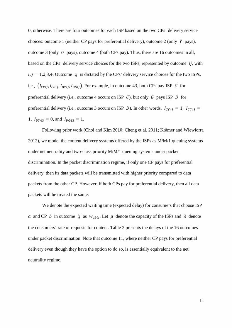
0, otherwise. There are four outcomes for each ISP based on the two CPs’ delivery service

choices: outcome 1 (neither CP pays for preferential delivery), outcome 2 (only 𝑌𝑌 pays),

outcome 3 (only 𝐺𝐺 pays), outcome 4 (both CPs pay). Thus, there are 16 outcomes in all,

based on the CPs’ delivery service choices for the two ISPs, represented by outcome 𝑖𝑖𝑗𝑗, with

𝑖𝑖, 𝑗𝑗 = 1,2,3,4. Outcome 𝑖𝑖𝑗𝑗 is dictated by the CPs’ delivery service choices for the two ISPs,

i.e., �𝐼𝐼𝐶𝐶𝑎𝑎𝑎𝑎𝑎𝑎 , 𝐼𝐼𝐶𝐶𝑎𝑎𝑎𝑎𝑎𝑎 , 𝐼𝐼𝐷𝐷𝑎𝑎𝑎𝑎𝑎𝑎 , 𝐼𝐼𝐷𝐷𝑎𝑎𝑎𝑎𝑎𝑎�. For example, in outcome 43, both CPs pay ISP 𝐶𝐶 for

preferential delivery (i.e., outcome 4 occurs on ISP 𝐶𝐶), but only 𝐺𝐺 pays ISP 𝐷𝐷 for

preferential delivery (i.e., outcome 3 occurs on ISP 𝐷𝐷). In other words, 𝐼𝐼𝐶𝐶𝑎𝑎43 = 1, 𝐼𝐼𝐶𝐶𝑎𝑎43 =

1, 𝐼𝐼𝐷𝐷𝑎𝑎43 = 0, and 𝐼𝐼𝐷𝐷𝑎𝑎43 = 1.

Following prior work (Choi and Kim 2010; Cheng et al. 2011; Krämer and Wiewiorra

2012), we model the content delivery systems offered by the ISPs as M/M/1 queuing systems

under net neutrality and two-class priority M/M/1 queuing systems under packet

discrimination. In the packet discrimination regime, if only one CP pays for preferential

delivery, then its data packets will be transmitted with higher priority compared to data

packets from the other CP. However, if both CPs pay for preferential delivery, then all data

packets will be treated the same.

We denote the expected waiting time (expected delay) for consumers that choose ISP

𝑎𝑎 and CP 𝑏𝑏 in outcome 𝑖𝑖𝑗𝑗 as 𝑤𝑤𝑎𝑎𝑎𝑎𝑎𝑎𝑎𝑎. Let 𝜇𝜇 denote the capacity of the ISPs and 𝜆𝜆 denote

the consumers’ rate of requests for content. Table 2 presents the delays of the 16 outcomes

under packet discrimination. Note that outcome 11, where neither CP pays for preferential

delivery even though they have the option to do so, is essentially equivalent to the net

neutrality regime.

11

Table 2: Delays under Packet Discrimination

Delays Neither pays 𝐷𝐷 𝑌𝑌 pays 𝐷𝐷 𝐺𝐺 pays 𝐷𝐷 Both pay 𝐷𝐷 Neither pays 𝐶𝐶

𝑤𝑤𝐶𝐶𝑎𝑎11 = 𝑤𝑤𝐶𝐶𝑎𝑎11 = 𝑤𝑤𝐷𝐷𝑎𝑎11 = 𝑤𝑤𝐷𝐷𝑎𝑎11=

1𝜇𝜇 − 𝑁𝑁𝐶𝐶𝑎𝑎11𝜆𝜆

𝑤𝑤𝐶𝐶𝑎𝑎12 = 𝑤𝑤𝐶𝐶𝑎𝑎12 =

1𝜇𝜇 − 𝑁𝑁𝐶𝐶12𝜆𝜆

𝑤𝑤𝐷𝐷𝑎𝑎12 =1

𝜇𝜇 − 𝑁𝑁𝐷𝐷𝑎𝑎12𝜆𝜆

𝑤𝑤𝐷𝐷𝑎𝑎12 =𝜇𝜇

(𝜇𝜇 − 𝑁𝑁𝐷𝐷𝑎𝑎12𝜆𝜆)(𝜇𝜇 − 𝑁𝑁𝐷𝐷12𝜆𝜆)

𝑤𝑤𝐶𝐶𝑎𝑎13 = 𝑤𝑤𝐶𝐶𝑎𝑎13 =1

𝜇𝜇 − 𝑁𝑁𝐶𝐶13𝜆𝜆

𝑤𝑤𝐷𝐷𝑎𝑎13 =𝜇𝜇

(𝜇𝜇 − 𝑁𝑁𝐷𝐷𝑎𝑎13𝜆𝜆)(𝜇𝜇 − 𝑁𝑁𝐷𝐷13𝜆𝜆)

𝑤𝑤𝐷𝐷𝑎𝑎13 =1

𝜇𝜇 − 𝑁𝑁𝐷𝐷𝑎𝑎13𝜆𝜆

𝑤𝑤𝐶𝐶𝑎𝑎14 = 𝑤𝑤𝐶𝐶𝑎𝑎14 = 𝑤𝑤𝐷𝐷𝑎𝑎14 = 𝑤𝑤𝐷𝐷𝑎𝑎14=

1𝜇𝜇 − 𝑁𝑁𝐶𝐶𝑎𝑎14𝜆𝜆

𝑌𝑌 pays 𝐶𝐶 𝑤𝑤𝐶𝐶𝑎𝑎21 =1

𝜇𝜇 − 𝑁𝑁𝐶𝐶𝑎𝑎21𝜆𝜆

𝑤𝑤𝐶𝐶𝑎𝑎21 =𝜇𝜇

(𝜇𝜇 − 𝑁𝑁𝐶𝐶𝑎𝑎21𝜆𝜆)(𝜇𝜇 − 𝑁𝑁𝐶𝐶21𝜆𝜆)

𝑤𝑤𝐷𝐷𝑎𝑎21 = 𝑤𝑤𝐷𝐷𝑎𝑎21 =1

𝜇𝜇 − 𝑁𝑁𝐷𝐷21𝜆𝜆

𝑤𝑤𝐶𝐶𝑎𝑎22 = 𝑤𝑤𝐷𝐷𝑎𝑎22 =1

𝜇𝜇 − 𝑁𝑁𝐶𝐶𝑎𝑎22𝜆𝜆

𝑤𝑤𝐶𝐶𝑎𝑎22 = 𝑤𝑤𝐷𝐷𝑎𝑎22=

𝜇𝜇(𝜇𝜇 − 𝑁𝑁𝐶𝐶𝑎𝑎22𝜆𝜆)(𝜇𝜇 − 𝑁𝑁𝐶𝐶22𝜆𝜆)

𝑤𝑤𝐶𝐶𝑎𝑎23 =1

𝜇𝜇 − 𝑁𝑁𝐶𝐶𝑎𝑎23𝜆𝜆

𝑤𝑤𝐶𝐶𝑎𝑎23 =𝜇𝜇

(𝜇𝜇 − 𝑁𝑁𝐶𝐶𝑎𝑎23𝜆𝜆)(𝜇𝜇 − 𝑁𝑁𝐶𝐶23𝜆𝜆)

𝑤𝑤𝐷𝐷𝑎𝑎23 =𝜇𝜇

(𝜇𝜇 − 𝑁𝑁𝐷𝐷𝑎𝑎23𝜆𝜆)(𝜇𝜇 − 𝑁𝑁𝐷𝐷23𝜆𝜆)

𝑤𝑤𝐷𝐷𝑎𝑎23 =1

𝜇𝜇 − 𝑁𝑁𝐷𝐷𝑎𝑎23𝜆𝜆

𝑤𝑤𝐶𝐶𝑎𝑎24 =1

𝜇𝜇 − 𝑁𝑁𝐶𝐶𝑎𝑎24𝜆𝜆

𝑤𝑤𝐶𝐶𝑎𝑎24 =𝜇𝜇

(𝜇𝜇 − 𝑁𝑁𝐶𝐶𝑎𝑎24𝜆𝜆)(𝜇𝜇 − 𝑁𝑁𝐶𝐶24𝜆𝜆)

𝑤𝑤𝐷𝐷𝑎𝑎24 = 𝑤𝑤𝐷𝐷𝑎𝑎24 =1

𝜇𝜇 − 𝑁𝑁𝐷𝐷24𝜆𝜆

𝐺𝐺 pays 𝐶𝐶 𝑤𝑤𝐶𝐶𝑎𝑎31 =𝜇𝜇

(𝜇𝜇 − 𝑁𝑁𝐶𝐶𝑎𝑎31𝜆𝜆)(𝜇𝜇 − 𝑁𝑁𝐶𝐶31𝜆𝜆)

𝑤𝑤𝐶𝐶𝑎𝑎31 =1

𝜇𝜇 − 𝑁𝑁𝐶𝐶𝑎𝑎31𝜆𝜆

𝑤𝑤𝐷𝐷𝑎𝑎31 = 𝑤𝑤𝐷𝐷𝑎𝑎31 =1

𝜇𝜇 − 𝑁𝑁𝐷𝐷31𝜆𝜆

𝑤𝑤𝐶𝐶𝑎𝑎32 =𝜇𝜇

(𝜇𝜇 − 𝑁𝑁𝐶𝐶𝑎𝑎32𝜆𝜆)(𝜇𝜇 − 𝑁𝑁𝐶𝐶32𝜆𝜆)

𝑤𝑤𝐶𝐶𝑎𝑎32 =1

𝜇𝜇 − 𝑁𝑁𝐶𝐶𝑎𝑎32𝜆𝜆

𝑤𝑤𝐷𝐷𝑎𝑎32 =1

𝜇𝜇 − 𝑁𝑁𝐷𝐷𝑎𝑎32𝜆𝜆

𝑤𝑤𝐷𝐷𝑎𝑎32 =𝜇𝜇

(𝜇𝜇 − 𝑁𝑁𝐷𝐷𝑎𝑎32𝜆𝜆)(𝜇𝜇 − 𝑁𝑁𝐷𝐷32𝜆𝜆)

𝑤𝑤𝐶𝐶𝑎𝑎33 = 𝑤𝑤𝐷𝐷𝑎𝑎33=

𝜇𝜇(𝜇𝜇 − 𝑁𝑁𝐶𝐶𝑎𝑎33𝜆𝜆)(𝜇𝜇 − 𝑁𝑁𝐶𝐶33𝜆𝜆)

𝑤𝑤𝐶𝐶𝑎𝑎33 = 𝑤𝑤𝐷𝐷𝑎𝑎33 =1

𝜇𝜇 − 𝑁𝑁𝐶𝐶𝑎𝑎33𝜆𝜆

𝑤𝑤𝐶𝐶𝑎𝑎34 =𝜇𝜇

(𝜇𝜇 − 𝑁𝑁𝐶𝐶𝑎𝑎34𝜆𝜆)(𝜇𝜇 − 𝑁𝑁𝐶𝐶34𝜆𝜆)

𝑤𝑤𝐶𝐶𝑎𝑎34 =1

𝜇𝜇 − 𝑁𝑁𝐶𝐶𝑎𝑎34𝜆𝜆

𝑤𝑤𝐷𝐷𝑎𝑎34 = 𝑤𝑤𝐷𝐷𝑎𝑎34 =1

𝜇𝜇 − 𝑁𝑁𝐷𝐷34𝜆𝜆

Both pay 𝐶𝐶

𝑤𝑤𝐶𝐶𝑎𝑎41 = 𝑤𝑤𝐶𝐶𝑎𝑎41 = 𝑤𝑤𝐷𝐷𝑎𝑎41 = 𝑤𝑤𝐷𝐷𝑎𝑎41=

1𝜇𝜇 − 𝑁𝑁𝐶𝐶𝑎𝑎41𝜆𝜆

𝑤𝑤𝐶𝐶𝑎𝑎42 = 𝑤𝑤𝐶𝐶𝑎𝑎42 =

1𝜇𝜇 − 𝑁𝑁𝐶𝐶42𝜆𝜆

𝑤𝑤𝐷𝐷𝑎𝑎42 =1

𝜇𝜇 − 𝑁𝑁𝐷𝐷𝑎𝑎42𝜆𝜆

𝑤𝑤𝐷𝐷𝑎𝑎42 =𝜇𝜇

(𝜇𝜇 − 𝑁𝑁𝐷𝐷𝑎𝑎42𝜆𝜆)(𝜇𝜇 − 𝑁𝑁𝐷𝐷42𝜆𝜆)

𝑤𝑤𝐶𝐶𝑎𝑎43 = 𝑤𝑤𝐶𝐶𝑎𝑎43 =1

𝜇𝜇 − 𝑁𝑁𝐶𝐶43𝜆𝜆

𝑤𝑤𝐷𝐷𝑎𝑎43 =𝜇𝜇

(𝜇𝜇 − 𝑁𝑁𝐷𝐷𝑎𝑎43𝜆𝜆)(𝜇𝜇 − 𝑁𝑁𝐷𝐷43𝜆𝜆)

𝑤𝑤𝐷𝐷𝑎𝑎43 =1

𝜇𝜇 − 𝑁𝑁𝐷𝐷𝑎𝑎43𝜆𝜆

𝑤𝑤𝐶𝐶𝑎𝑎44 = 𝑤𝑤𝐶𝐶𝑎𝑎44 = 𝑤𝑤𝐷𝐷𝑎𝑎44 = 𝑤𝑤𝐷𝐷𝑎𝑎44=

1𝜇𝜇 − 𝑁𝑁𝐶𝐶𝑎𝑎44𝜆𝜆

12

In summary, the consumers’ utility functions for the four ISP-CP combinations are:

𝑢𝑢𝐶𝐶𝑎𝑎𝑎𝑎𝑎𝑎(𝑥𝑥, 𝑧𝑧) = 𝑉𝑉 − 𝑡𝑡𝑥𝑥 − 𝑘𝑘𝑧𝑧 − 𝑑𝑑𝜆𝜆𝑤𝑤𝐶𝐶𝑎𝑎𝑎𝑎𝑎𝑎 − 𝐹𝐹𝐶𝐶𝑎𝑎𝑎𝑎

𝑢𝑢𝐶𝐶𝑎𝑎𝑎𝑎𝑎𝑎(𝑥𝑥, 𝑧𝑧) = 𝑉𝑉 − 𝑡𝑡(1 − 𝑥𝑥) − 𝑘𝑘𝑧𝑧 − 𝑑𝑑𝜆𝜆𝑤𝑤𝐶𝐶𝑎𝑎𝑎𝑎𝑎𝑎 − 𝐹𝐹𝐶𝐶𝑎𝑎𝑎𝑎

𝑢𝑢𝐷𝐷𝑎𝑎𝑎𝑎𝑎𝑎(𝑥𝑥, 𝑧𝑧) = 𝑉𝑉 − 𝑡𝑡𝑥𝑥 − 𝑘𝑘(1 − 𝑧𝑧) − 𝑑𝑑𝜆𝜆𝑤𝑤𝐷𝐷𝑎𝑎𝑎𝑎𝑎𝑎 − 𝐹𝐹𝐷𝐷𝑎𝑎𝑎𝑎

𝑢𝑢𝐷𝐷𝑎𝑎𝑎𝑎𝑎𝑎(𝑥𝑥, 𝑧𝑧) = 𝑉𝑉 − 𝑡𝑡(1 − 𝑥𝑥) − 𝑘𝑘(1 − 𝑧𝑧) − 𝑑𝑑𝜆𝜆𝑤𝑤𝐶𝐶𝑎𝑎𝑎𝑎𝑎𝑎 − 𝐹𝐹𝐷𝐷𝑎𝑎𝑎𝑎

where 𝑑𝑑 represents the consumers’ unit delay cost (congestion cost).

Each consumer compares the four ISP-CP combinations and chooses the option that

yields the highest utility. We denote the market share of the ISP-CP combination 𝑎𝑎𝑏𝑏 in

outcome 𝑖𝑖𝑗𝑗 as 𝑁𝑁𝑎𝑎𝑎𝑎𝑎𝑎𝑎𝑎. For example, 𝑁𝑁𝐷𝐷𝑎𝑎43 represents the market share of 𝐷𝐷𝐺𝐺 when both

CPs pay ISP 𝐶𝐶 but only 𝐺𝐺 pays ISP 𝐷𝐷.

CPs decide whether to pay ISP 𝐶𝐶, ISP 𝐷𝐷, or both. The profit of CP 𝑏𝑏 = 𝑌𝑌 or 𝐺𝐺 is:

𝜋𝜋𝑎𝑎𝑎𝑎𝑎𝑎 = �𝑁𝑁𝐶𝐶𝑎𝑎𝑎𝑎𝑎𝑎 + 𝑁𝑁𝐷𝐷𝑎𝑎𝑎𝑎𝑎𝑎�𝜆𝜆𝑟𝑟𝑎𝑎 − 𝐼𝐼𝐶𝐶𝑎𝑎𝑎𝑎𝑎𝑎𝑁𝑁𝐶𝐶𝑎𝑎𝑎𝑎𝑎𝑎𝜆𝜆𝑝𝑝𝐶𝐶𝑎𝑎𝑎𝑎 − 𝐼𝐼𝐷𝐷𝑎𝑎𝑎𝑎𝑎𝑎𝑁𝑁𝐷𝐷𝑎𝑎𝑎𝑎𝑎𝑎𝜆𝜆𝑝𝑝𝐷𝐷𝑎𝑎𝑎𝑎

where 𝑟𝑟𝑎𝑎 is the revenue rate per packet of CP 𝑏𝑏. The CPs’ profit is their revenue generated

from consumers served by both ISPs, net of their payments to the ISPs for preferential

content delivery. Without loss of generality, we assume that 𝑟𝑟𝑎𝑎 ≥ 𝑟𝑟𝑎𝑎, or, CP 𝐺𝐺 is more

effective in generating revenue from its customer base than is CP 𝑌𝑌.

ISPs make their pricing decisions. ISP 𝑎𝑎 = 𝐶𝐶 or 𝐷𝐷 selects its prices 𝐹𝐹𝑎𝑎𝑎𝑎𝑎𝑎 and 𝑝𝑝𝑎𝑎𝑎𝑎𝑎𝑎

to maximize its profit 𝜋𝜋𝑎𝑎𝑎𝑎𝑎𝑎. The decision problem of ISP 𝑎𝑎 can be formulated as:

max𝐹𝐹𝑎𝑎𝑎𝑎𝑎𝑎 ,𝑝𝑝𝑎𝑎𝑎𝑎𝑎𝑎

𝜋𝜋𝑎𝑎𝑎𝑎𝑎𝑎 = �𝑁𝑁𝑎𝑎𝑎𝑎𝑎𝑎𝑎𝑎 + 𝑁𝑁𝑎𝑎𝑎𝑎𝑎𝑎𝑎𝑎�𝐹𝐹𝑎𝑎𝑎𝑎𝑎𝑎 + �𝐼𝐼𝑎𝑎𝑎𝑎𝑎𝑎𝑎𝑎𝑁𝑁𝑎𝑎𝑎𝑎𝑎𝑎𝑎𝑎 + 𝐼𝐼𝑎𝑎𝑎𝑎𝑎𝑎𝑎𝑎𝑁𝑁𝑎𝑎𝑎𝑎𝑎𝑎𝑎𝑎�𝜆𝜆𝑝𝑝𝑎𝑎𝑎𝑎𝑎𝑎

subject to 𝑈𝑈𝑎𝑎𝑎𝑎(𝑥𝑥, 𝑧𝑧) = max�𝑢𝑢𝐶𝐶𝑎𝑎𝑎𝑎𝑎𝑎(𝑥𝑥, 𝑧𝑧),𝑢𝑢𝐶𝐶𝑎𝑎𝑎𝑎𝑎𝑎(𝑥𝑥, 𝑧𝑧),𝑢𝑢𝐷𝐷𝑎𝑎𝑎𝑎𝑎𝑎(𝑥𝑥, 𝑧𝑧),𝑢𝑢𝐷𝐷𝑎𝑎𝑎𝑎𝑎𝑎(𝑥𝑥, 𝑧𝑧)� ≥ 0

𝜋𝜋𝑎𝑎𝑎𝑎𝑎𝑎 ≥ 𝜋𝜋𝑎𝑎𝑎𝑎1𝑎𝑎1 ,𝜋𝜋𝑎𝑎𝑎𝑎2𝑎𝑎2 ,𝜋𝜋𝑎𝑎𝑎𝑎3𝑎𝑎3

𝜋𝜋𝑎𝑎𝑎𝑎𝑎𝑎 ≥ 𝜋𝜋𝑎𝑎𝑎𝑎4𝑎𝑎4 ,𝜋𝜋𝑎𝑎𝑎𝑎5𝑎𝑎5 ,𝜋𝜋𝑎𝑎𝑎𝑎6𝑎𝑎6.

The ISPs’ profit consists of two components: payment from consumers for Internet

access service and payment from CPs for preferential content delivery. The first constraint is

13

consumers’ participation constraint. Consumers choose the ISP-CP combination that yields

the highest net utility, and consumers’ participation constraint ensures that all consumers

adopt the Internet access service. This full-market-coverage assumption is commonly made in

the literature (Choi and Kim 2010; Guo et al. 2010; Cheng et al. 2011). The last two

constraints are the CPs’ incentive compatibility constraints. In response to the prices (𝐹𝐹𝑎𝑎𝑎𝑎𝑎𝑎

and 𝑝𝑝𝑎𝑎𝑎𝑎𝑎𝑎) set by the ISPs, the CPs choose whether to pay for preferential delivery and their

choices of content delivery services determine the outcomes 𝑖𝑖𝑗𝑗 for both ISPs.

The CPs’ incentive compatibility constraints ensure that neither CP has any incentive

to deviate from outcome 𝑖𝑖𝑗𝑗. In other words, given the other CP’s delivery service choice, the

profit for a CP in outcome 𝑖𝑖𝑗𝑗 needs to be higher than that with its alternative choices.

Outcomes 𝑖𝑖1𝑗𝑗1, 𝑖𝑖2𝑗𝑗2, 𝑖𝑖3𝑗𝑗3 represent 𝑌𝑌’s alternative choices and 𝑖𝑖4𝑗𝑗4, 𝑖𝑖5𝑗𝑗5, 𝑖𝑖6𝑗𝑗6 represent 𝐺𝐺’s

alternative choices. For example, for outcome 43 (both CPs pay ISP 𝐶𝐶 and only 𝐺𝐺 pays ISP

𝐷𝐷) to be an equilibrium, there are three conditions for each CP’s incentive compatibility

constraint. Given that 𝐺𝐺 pays both ISPs in outcome 43, 𝑌𝑌 has three options: (1) not pay

either ISP (outcome 33); (2) pay both ISPs (outcome 44); or (3) not pay ISP 𝐶𝐶 but pay ISP

𝐷𝐷 (outcome 34). Similarly, Given 𝑌𝑌’s payment choice in outcome 43 (it pays 𝐶𝐶 but not 𝐷𝐷),

𝐺𝐺 also has three options: (1) not pay 𝐶𝐶 but pay 𝐷𝐷 (outcome 23); (2) pay 𝐶𝐶 but not pay 𝐷𝐷

(outcome 41); or (3) not pay either ISP (outcome 21). Formally, 𝑖𝑖1𝑗𝑗1,⋯ , 𝑖𝑖6𝑗𝑗6 are defined by

the following CPs’ decisions: 𝑖𝑖1𝑗𝑗1 ↔ �1 − 𝐼𝐼𝐶𝐶𝑎𝑎𝑎𝑎𝑎𝑎, 𝐼𝐼𝐶𝐶𝑎𝑎𝑎𝑎𝑎𝑎 , 𝐼𝐼𝐷𝐷𝑎𝑎𝑎𝑎𝑎𝑎, 𝐼𝐼𝐷𝐷𝑎𝑎𝑎𝑎𝑎𝑎�, 𝑖𝑖2𝑗𝑗2 ↔ �𝐼𝐼𝐶𝐶𝑎𝑎𝑎𝑎𝑎𝑎 , 𝐼𝐼𝐶𝐶𝑎𝑎𝑎𝑎𝑎𝑎 , 1 −

𝐼𝐼𝐷𝐷𝑎𝑎𝑎𝑎𝑎𝑎 , 𝐼𝐼𝐷𝐷𝑎𝑎𝑎𝑎𝑎𝑎�, 𝑖𝑖3𝑗𝑗3 ↔ �1 − 𝐼𝐼𝐶𝐶𝑎𝑎𝑎𝑎𝑎𝑎 , 𝐼𝐼𝐶𝐶𝑎𝑎𝑎𝑎𝑎𝑎 , 1 − 𝐼𝐼𝐷𝐷𝑎𝑎𝑎𝑎𝑎𝑎, 𝐼𝐼𝐷𝐷𝑎𝑎𝑎𝑎𝑎𝑎�, 𝑖𝑖4𝑗𝑗4 ↔ �𝐼𝐼𝐶𝐶𝑎𝑎𝑎𝑎𝑎𝑎 , 1 − 𝐼𝐼𝐶𝐶𝑎𝑎𝑎𝑎𝑎𝑎 , 𝐼𝐼𝐷𝐷𝑎𝑎𝑎𝑎𝑎𝑎 , 𝐼𝐼𝐷𝐷𝑎𝑎𝑎𝑎𝑎𝑎�,

𝑖𝑖5𝑗𝑗5 ↔ �𝐼𝐼𝐶𝐶𝑎𝑎𝑎𝑎𝑎𝑎 , 𝐼𝐼𝐶𝐶𝑎𝑎𝑎𝑎𝑎𝑎 , 𝐼𝐼𝐷𝐷𝑎𝑎𝑎𝑎𝑎𝑎 , 1 − 𝐼𝐼𝐷𝐷𝑎𝑎𝑎𝑎𝑎𝑎�, and 𝑖𝑖6𝑗𝑗6 ↔ �𝐼𝐼𝐶𝐶𝑎𝑎𝑎𝑎𝑎𝑎, 1 − 𝐼𝐼𝐶𝐶𝑎𝑎𝑎𝑎𝑎𝑎 , 𝐼𝐼𝐷𝐷𝑎𝑎𝑎𝑎𝑎𝑎 , 1 − 𝐼𝐼𝐷𝐷𝑎𝑎𝑎𝑎𝑎𝑎�. The

details of the CPs’ incentive compatibility constraints are presented in Table 3.

14

Table 3: CPs’ Incentive Compatibility Constraints

IC constraints Neither pays 𝐷𝐷 𝑌𝑌 pays 𝐷𝐷 𝐺𝐺 pays 𝐷𝐷 Both pay 𝐷𝐷

Neither pays 𝐶𝐶

𝜋𝜋𝑎𝑎11≥ 𝜋𝜋𝑎𝑎21,𝜋𝜋𝑎𝑎12,𝜋𝜋𝑎𝑎22 𝜋𝜋𝑎𝑎11≥ 𝜋𝜋𝑎𝑎31,𝜋𝜋𝑎𝑎13,𝜋𝜋𝑎𝑎33

𝜋𝜋𝑎𝑎12≥ 𝜋𝜋𝑎𝑎22,𝜋𝜋𝑎𝑎11,𝜋𝜋𝑎𝑎21 𝜋𝜋𝑎𝑎12≥ 𝜋𝜋𝑎𝑎32,𝜋𝜋𝑎𝑎14,𝜋𝜋𝑎𝑎34

𝜋𝜋𝑎𝑎13≥ 𝜋𝜋𝑎𝑎23,𝜋𝜋𝑎𝑎14,𝜋𝜋𝑎𝑎24 𝜋𝜋𝑎𝑎13≥ 𝜋𝜋𝑎𝑎33,𝜋𝜋𝑎𝑎11,𝜋𝜋𝑎𝑎31

𝜋𝜋𝑎𝑎14≥ 𝜋𝜋𝑎𝑎24,𝜋𝜋𝑎𝑎13,𝜋𝜋𝑎𝑎23 𝜋𝜋𝑎𝑎14≥ 𝜋𝜋𝑎𝑎34,𝜋𝜋𝑎𝑎12,𝜋𝜋𝑎𝑎32

𝑌𝑌 pays 𝐶𝐶

𝜋𝜋𝑎𝑎21≥ 𝜋𝜋𝑎𝑎11,𝜋𝜋𝑎𝑎22,𝜋𝜋𝑎𝑎12 𝜋𝜋𝑎𝑎21≥ 𝜋𝜋𝑎𝑎41,𝜋𝜋𝑎𝑎23,𝜋𝜋𝑎𝑎43

𝜋𝜋𝑎𝑎22≥ 𝜋𝜋𝑎𝑎12,𝜋𝜋𝑎𝑎21,𝜋𝜋𝑎𝑎11 𝜋𝜋𝑎𝑎22≥ 𝜋𝜋𝑎𝑎42,𝜋𝜋𝑎𝑎24,𝜋𝜋𝑎𝑎44

𝜋𝜋𝑎𝑎23≥ 𝜋𝜋𝑎𝑎13,𝜋𝜋𝑎𝑎24,𝜋𝜋𝑎𝑎14 𝜋𝜋𝑎𝑎23≥ 𝜋𝜋𝑎𝑎43,𝜋𝜋𝑎𝑎21,𝜋𝜋𝑎𝑎41

𝜋𝜋𝑎𝑎24≥ 𝜋𝜋𝑎𝑎14,𝜋𝜋𝑎𝑎23,𝜋𝜋𝑎𝑎13 𝜋𝜋𝑎𝑎24≥ 𝜋𝜋𝑎𝑎44,𝜋𝜋𝑎𝑎22,𝜋𝜋𝑎𝑎42

𝐺𝐺 pays 𝐶𝐶

𝜋𝜋𝑎𝑎31≥ 𝜋𝜋𝑎𝑎41,𝜋𝜋𝑎𝑎32,𝜋𝜋𝑎𝑎42 𝜋𝜋𝑎𝑎31≥ 𝜋𝜋𝑎𝑎11,𝜋𝜋𝑎𝑎33,𝜋𝜋𝑎𝑎13

𝜋𝜋𝑎𝑎32≥ 𝜋𝜋𝑎𝑎42,𝜋𝜋𝑎𝑎31,𝜋𝜋𝑎𝑎41 𝜋𝜋𝑎𝑎32≥ 𝜋𝜋𝑎𝑎12,𝜋𝜋𝑎𝑎34,𝜋𝜋𝑎𝑎14

𝜋𝜋𝑎𝑎33≥ 𝜋𝜋𝑎𝑎43,𝜋𝜋𝑎𝑎34,𝜋𝜋𝑎𝑎44 𝜋𝜋𝑎𝑎33≥ 𝜋𝜋𝑎𝑎13,𝜋𝜋𝑎𝑎31,𝜋𝜋𝑎𝑎11

𝜋𝜋𝑎𝑎34≥ 𝜋𝜋𝑎𝑎44,𝜋𝜋𝑎𝑎33,𝜋𝜋𝑎𝑎43 𝜋𝜋𝑎𝑎34≥ 𝜋𝜋𝑎𝑎14,𝜋𝜋𝑎𝑎32,𝜋𝜋𝑎𝑎12

Both pay 𝐶𝐶

𝜋𝜋𝑎𝑎41≥ 𝜋𝜋𝑎𝑎31,𝜋𝜋𝑎𝑎42,𝜋𝜋𝑎𝑎32 𝜋𝜋𝑎𝑎41≥ 𝜋𝜋𝑎𝑎21,𝜋𝜋𝑎𝑎43,𝜋𝜋𝑎𝑎23

𝜋𝜋𝑎𝑎42≥ 𝜋𝜋𝑎𝑎32,𝜋𝜋𝑎𝑎41,𝜋𝜋𝑎𝑎31 𝜋𝜋𝑎𝑎42≥ 𝜋𝜋𝑎𝑎22,𝜋𝜋𝑎𝑎44,𝜋𝜋𝑎𝑎24

𝜋𝜋𝑎𝑎43≥ 𝜋𝜋𝑎𝑎33,𝜋𝜋𝑎𝑎44,𝜋𝜋𝑎𝑎34 𝜋𝜋𝑎𝑎43≥ 𝜋𝜋𝑎𝑎23,𝜋𝜋𝑎𝑎41,𝜋𝜋𝑎𝑎21

𝜋𝜋𝑎𝑎44≥ 𝜋𝜋𝑎𝑎34,𝜋𝜋𝑎𝑎43,𝜋𝜋𝑎𝑎33 𝜋𝜋𝑎𝑎44≥ 𝜋𝜋𝑎𝑎24,𝜋𝜋𝑎𝑎42,𝜋𝜋𝑎𝑎22

The sequence of decisions is as follows: In stage 1, ISPs 𝑎𝑎 = 𝐶𝐶 or 𝐷𝐷 set the fixed fee

𝐹𝐹𝑎𝑎 for end consumers and potentially a priority price of 𝑝𝑝𝑎𝑎 per packet. In stage 2, CPs 𝑏𝑏 =

𝑌𝑌 or 𝐺𝐺 decides whether to pay or not pay the ISPs 𝐶𝐶 and 𝐷𝐷 for preferential delivery of

their content. In stage 3, consumers choose their preferred CP and ISP. In the following

section, we solve for the symmetric equilibria in this game.

ANALYSIS OF NET NEUTRALITY AND PACKET DISCRIMINATION REGIMES

Consumers compare the four ISP-CP options and choose the option which yields the highest

utility. In order to derive the market shares for each option, we need to calculate the six

indifference curves based on the pairwise comparisons among them. Figure 3 demonstrates

the various possibilities of how consumers are distributed among the four options. Solving for

the exact market shares under each ISP-CP combination is difficult, since (1) there is a surfeit

of parameter values; (2) we model the packet discrimination system as a priority queue, so 15

the waiting times are a rational function of all the parameters; and (3) several of the variables

are implicitly interrelated (for example, the waiting times are functions of consumer demand,

which is dependent on the indifferent curves, that are in turn determined by the waiting times,

and in general there is no closed-form solution for these implicit relations). Thus, the market

shares under each ISP-CP option could look very different; see the dotted lines in Figure 3 as

a possible example.

In order to solve this problem, we utilize the symmetry of the corresponding market

shares when the content providers interchange their decisions on prioritizing their content

delivery. For example, if the decisions of 𝑌𝑌 and 𝐺𝐺 are simultaneously changed for ISPs 𝐶𝐶

and 𝐷𝐷, the market shares under each ISP-CP option “flips”. Depending on the shape of the

“flipped” market shares, there are two types of flips – “horizontal” or “vertical”.

Interchanging the business decisions of the CPs (vertical and horizontal flips) induces what is

called a ℤ2 × ℤ2 (or the Klein 4-group) action in group theory. We use the symmetry

associated with this group action to solve for the demand distributions. The details of this

symmetry analysis using vertical and horizontal flips can be found in the appendix. The

results of the consumer demand patterns are summarized in Lemma 1. All proofs are

relegated to the appendix.

Figure 3: General Demand Distribution

𝐷𝐷𝑌𝑌 𝐷𝐷𝐺𝐺

𝐶𝐶𝐺𝐺 𝐶𝐶𝑌𝑌

𝐷𝐷𝑌𝑌 𝐷𝐷𝐺𝐺

𝐶𝐶𝐺𝐺 𝐶𝐶𝑌𝑌

𝐷𝐷𝑌𝑌 𝐷𝐷𝐺𝐺

𝐶𝐶𝐺𝐺 𝐶𝐶𝑌𝑌

16

Lemma 1 (Consumer Demand Patterns): Depending on the ISPs’ pricing decisions and the

content providers’ delivery service choices, there are 16 possible outcomes. These outcomes

can be grouped into four classes (a through d) with similar consumer demand patterns.

Figure 4 portrays the results in Lemma 1. For outcomes 𝑖𝑖𝑗𝑗 = 11,14, 41,44 in class a,

all data packets receive equal priority and thus consumers incur the same congestion cost. As

shown in Figure 4a, the four ISP-CP combinations split the consumer market equally, i.e.,

𝑁𝑁𝐶𝐶𝑎𝑎𝑎𝑎𝑎𝑎 = 𝑁𝑁𝐶𝐶𝑎𝑎𝑎𝑎𝑎𝑎 = 𝑁𝑁𝐷𝐷𝑎𝑎𝑎𝑎𝑎𝑎 = 𝑁𝑁𝐷𝐷𝑎𝑎𝑎𝑎𝑎𝑎 = 1 4⁄ .

Figure 4a: Demand Distribution of Class a (outcomes 11, 14, 41, and 44)

For outcomes 𝑖𝑖𝑗𝑗 = 22,33 in class b, the CPs make the same delivery service choices

with either ISP. As a result, ISPs 𝐶𝐶 and 𝐷𝐷 have the same market share, i.e., 𝑁𝑁𝐶𝐶𝑎𝑎𝑎𝑎 = 𝑁𝑁𝐷𝐷𝑎𝑎𝑎𝑎 =

1 2⁄ . Within each ISP, the paying CP gets more customers than the non-paying CP, i.e.,

𝑁𝑁𝐶𝐶𝑎𝑎22 = 𝑁𝑁𝐷𝐷𝑎𝑎22 = 𝑁𝑁𝐶𝐶𝑎𝑎33 = 𝑁𝑁𝐷𝐷𝑎𝑎33 ≥ 1 4⁄ ≥ 𝑁𝑁𝐶𝐶𝑎𝑎33 = 𝑁𝑁𝐷𝐷𝑎𝑎33 = 𝑁𝑁𝐶𝐶𝑎𝑎22 = 𝑁𝑁𝐷𝐷𝑎𝑎22.

𝐷𝐷𝑌𝑌 𝐷𝐷𝐺𝐺

𝐶𝐶𝐺𝐺 𝐶𝐶𝑌𝑌 1 2⁄

1 2⁄

17

Outcome 22 Outcome 33

Figure 4b: Demand Distribution of Class b (outcomes 22 and 33)

For outcomes 𝑖𝑖𝑗𝑗 = 23,32 in class c, the CPs make the opposite delivery service

choices with the two ISPs, leading to only one CP paying for the preferential delivery on each

ISP. As a result, ISPs 𝐶𝐶 and 𝐷𝐷 have the same market share, i.e., 𝑁𝑁𝐶𝐶𝑎𝑎𝑎𝑎 = 𝑁𝑁𝐷𝐷𝑎𝑎𝑎𝑎 = 1 2⁄ .

Within each ISP, the paying CP gets more customers than the non-paying CP, i.e., 𝑁𝑁𝐶𝐶𝑎𝑎23 =

𝑁𝑁𝐷𝐷𝑎𝑎23 = 𝑁𝑁𝐶𝐶𝑎𝑎32 = 𝑁𝑁𝐷𝐷𝑎𝑎32 ≥ 1 4⁄ ≥ 𝑁𝑁𝐶𝐶𝑎𝑎32 = 𝑁𝑁𝐷𝐷𝑎𝑎32 = 𝑁𝑁𝐶𝐶𝑎𝑎23 = 𝑁𝑁𝐷𝐷𝑎𝑎23.

Outcome 23 Outcome 32

Figure 4c: Demand Distribution of Class c (outcomes 23 and 32)

𝐷𝐷𝑌𝑌 𝐷𝐷𝐺𝐺

𝐶𝐶𝐺𝐺 𝐶𝐶𝑌𝑌 1 2⁄

1 2⁄

𝑥𝑥22

𝐷𝐷𝑌𝑌 𝐷𝐷𝐺𝐺

𝐶𝐶𝐺𝐺 𝐶𝐶𝑌𝑌 1 2⁄ 𝑥𝑥33

1 2⁄

𝐷𝐷𝑌𝑌 𝐷𝐷𝐺𝐺

𝐶𝐶𝐺𝐺 𝐶𝐶𝑌𝑌

1 2⁄

𝑧𝑧𝑎𝑎23

𝑧𝑧𝑎𝑎23

1 2⁄ 𝑥𝑥𝐶𝐶23

𝑥𝑥𝐷𝐷23 𝐷𝐷𝑌𝑌 𝐷𝐷𝐺𝐺

𝐶𝐶𝐺𝐺 𝐶𝐶𝑌𝑌

1 2⁄

𝑧𝑧𝑎𝑎32

𝑧𝑧𝑎𝑎32

1 2⁄ 𝑥𝑥𝐶𝐶32

𝑥𝑥𝐷𝐷32

18

For outcomes 𝑖𝑖𝑗𝑗 = 12,13,21,31,42,43,24,34 in class d, 𝑁𝑁𝐷𝐷𝑎𝑎𝑎𝑎 ≥ 1 2⁄ ≥ 𝑁𝑁𝐶𝐶𝑎𝑎𝑎𝑎 for

outcomes 𝑖𝑖𝑗𝑗 = 12,13,42,43 and 𝑁𝑁𝐶𝐶𝑎𝑎𝑎𝑎 ≥ 1 2⁄ ≥ 𝑁𝑁𝐷𝐷𝑎𝑎𝑎𝑎 for outcomes 𝑖𝑖𝑗𝑗 = 21,31,24,34.

Outcomes in class d reveal particularly interesting demand patterns. For example, in outcome

43, although both CPs pay for preferential delivery on ISP 𝐶𝐶, 𝑌𝑌 gets fewer consumers than

𝐺𝐺 from ISP 𝐶𝐶, i.e., 𝑁𝑁𝐶𝐶𝑎𝑎43 > 𝑁𝑁𝐶𝐶𝑎𝑎43.

Outcomes 12 and 42 Outcomes 13 and 43

Outcomes 21 and 24 Outcomes 31 and 34

Figure 4d: Demand Distribution of Class d

(outcomes 12, 13, 21, 31, 42, 43, 24, and 34)

𝐷𝐷𝑌𝑌 𝐷𝐷𝐺𝐺

𝐶𝐶𝐺𝐺 𝐶𝐶𝑌𝑌

1 2⁄

1 2⁄

𝑧𝑧𝑎𝑎42

𝑧𝑧𝑎𝑎42

𝐷𝐷𝑌𝑌 𝐷𝐷𝐺𝐺

𝐶𝐶𝐺𝐺 𝐶𝐶𝑌𝑌

1 2⁄

1 2⁄

𝑧𝑧𝑎𝑎43

𝑧𝑧𝑎𝑎43

𝑥𝑥𝐷𝐷43

𝐷𝐷𝑌𝑌 𝐷𝐷𝐺𝐺

𝐶𝐶𝐺𝐺 𝐶𝐶𝑌𝑌

1 2⁄

1 2⁄

𝑧𝑧𝑎𝑎24

𝑧𝑧𝑎𝑎24

𝑥𝑥𝐷𝐷24 𝐷𝐷𝑌𝑌 𝐷𝐷𝐺𝐺

𝐶𝐶𝐺𝐺 𝐶𝐶𝑌𝑌

1 2⁄

1 2⁄

𝑧𝑧𝑎𝑎34

𝑧𝑧𝑎𝑎34

𝑥𝑥𝐶𝐶34

19

Lemma 2 (ISPs’ Strategy): Depending on market conditions, there are three possible

symmetric equilibrium pricing strategies (i.e. the 𝐹𝐹 and 𝑝𝑝 choices) for the ISPs: (a) when

𝑟𝑟𝑎𝑎 ≥ 𝑚𝑚𝑎𝑎𝑥𝑥{𝛼𝛼1,𝛽𝛽1𝑟𝑟𝑎𝑎,𝛼𝛼2 + 𝛽𝛽2𝑟𝑟𝑎𝑎}, the equilibrium is outcome 33, where only content provider

G pays for priority delivery for its customers on both ISPs; (b) when 𝛽𝛽3𝑟𝑟𝑎𝑎 ≤ 𝑟𝑟𝑎𝑎 < 𝛼𝛼1 and

𝑟𝑟𝑎𝑎 ≤ 𝛼𝛼3, the equilibrium is outcome 43 (and equivalently, equilibrium 34), where content

provider 𝐺𝐺 pays for priority delivery for its customers on both ISPs, while Y pays for

priority delivery for its customers with only one ISP2; and (c) otherwise, the equilibrium is

outcome 44, where both content providers pay for priority delivery for their customers on

both ISPs.

We diagrammatically show the results of Lemma 2 in Figure 5a. The equilibrium

results assuming 𝑟𝑟𝑎𝑎 ≥ 𝑟𝑟𝑎𝑎 can be easily generalized to the case when 𝑟𝑟𝑎𝑎 < 𝑟𝑟𝑎𝑎. Figure 5b

shows the equilibrium outcomes when the assumption of 𝑟𝑟𝑎𝑎 ≥ 𝑟𝑟𝑎𝑎 is relaxed.

Figure 5a: Equilibrium outcomes when 𝑟𝑟𝑎𝑎 ≥ 𝑟𝑟𝑎𝑎

2 This equilibrium is equivalent to the one where 𝐺𝐺 pays for priority delivery to one ISP while 𝑌𝑌 pays for priority delivery to both ISPs, in the sense that the profits of the content providers is the same in either case.

𝑟𝑟𝑎𝑎 = 𝑟𝑟𝑎𝑎

𝑟𝑟𝑎𝑎

𝑟𝑟𝑎𝑎

33

43 or 34

44

20

Figure 5b: Equilibrium outcomes when the assumption 𝑟𝑟𝑎𝑎 ≥ 𝑟𝑟𝑎𝑎 is relaxed

Figure 5: Equilibrium Outcomes

In general, ISPs will charge higher prices to content providers when only one pays for

priority delivery than when both content providers pay for priority delivery. Consumers,

however, are charged less, indicating that as the revenue generation rate 𝑟𝑟𝑎𝑎 increases, the

relative contribution to ISPs’ profit gradually switches from consumers to the content

providers. This leads to our first proposition.

Proposition 1 (Competing ISPs still have an incentive to deviate from net neutrality):

The competing ISPs’ profit is weakly higher under packet discrimination than under net

neutrality, i.e., 𝜋𝜋𝐶𝐶𝑃𝑃𝐷𝐷 = 𝜋𝜋𝐷𝐷𝑃𝑃𝐷𝐷 ≥ 𝜋𝜋𝐶𝐶𝑁𝑁𝑁𝑁 = 𝜋𝜋𝐷𝐷𝑁𝑁𝑁𝑁.

Proposition 1 shows that the competing ISPs are always better off under packet

discrimination even in the presence of ISP competition and thus have the incentive to deviate

from net neutrality. In other words, when it comes to the net neutrality debate, ISPs will

prefer abolishing net neutrality, even in the presence of ISP competition. This is a result that

has been shown to be true when the ISP is a monopoly and it continues to hold with ISP

𝑟𝑟𝑎𝑎 = 𝑟𝑟𝑎𝑎

𝑟𝑟𝑎𝑎

𝑟𝑟𝑎𝑎

33

44

43 or 34

44

22 42 or 24

21

competition. This finding is different from that of Bourreau et al. (2014), where the authors

do not model the competition between content providers, and as a result, the effect of

competition faced by the ISPs is exaggerated. Our analysis provides an explanation for the

public stance of the Internet service providers in the ongoing net neutrality debate, as they

continue to lobby for abolishing net neutrality. This result mirrors the results of Gans (2014),

even though he does not explicitly model the effects of ISP competition.

Content providers, however, have supported the preservation of net neutrality. Would

they continue to support net neutrality when there is competition between ISPs? Our next

result (Proposition 2) shows that under certain conditions, it is economically beneficial for the

dominant content provider to reverse its stance on net neutrality. In other words, some

content providers might be better off when net neutrality is abolished in the presence of

competition between ISPs. This is a crucial and, in some ways, a surprising result. Ever since

the issue of net neutrality has been publicly debated, prominent content providers like Google,

Yahoo!, Microsoft, Netflix and others have publicly supported net neutrality, and so far, the

economic analyses have mirrored the public stances of the various parties in the debate:

content providers are worse off when net neutrality is abolished, while the Internet service

providers are better off. Proposition 2 shows that under ISP competition, the support for net

neutrality from content providers – and more specifically, from the dominant content

providers – might not be so forthcoming.

Proposition 2 (CP G may be better off under packet discrimination): When CP G is

sufficiently dominant, its profit is higher under packet discrimination (corresponds to

equilibrium 33) than that under net neutrality if the intensity of competition in the ISP market

relative to that in the CP market is greater than a threshold. Formally, 𝜋𝜋𝑎𝑎𝑃𝑃𝐷𝐷 = 𝜋𝜋𝑎𝑎33∗ > 𝜋𝜋𝑎𝑎𝑁𝑁𝑁𝑁

if the ratio of 𝑡𝑡 𝑘𝑘⁄ is higher than a threshold.

22

Proposition 2 shows that under certain conditions, CP 𝐺𝐺 might in fact do better than

it could under net neutrality. When 𝑟𝑟𝑎𝑎 and 𝑟𝑟𝑎𝑎 are similar and the corresponding equilibrium

outcome is 44 (both CPs decide to pay the two ISPs), CP 𝐺𝐺 is definitely worse off under

packet discrimination than under net neutrality. As 𝑟𝑟𝑎𝑎 becomes larger relative to 𝑟𝑟𝑎𝑎,

however, and the equilibrium shifts to outcome 33 (where only G prefers to pay the two ISPs),

𝐺𝐺’s profit is at least as great as that under net neutrality. Specifically, the comparison result of

𝐺𝐺’s profit depends on the relative magnitude of the intensity of competition in the ISP and CP

markets. We can think of the unit fit costs 𝑡𝑡 and 𝑘𝑘 as the strengths of the consumer

loyalties within the CP market and within the ISP market, respectively. A more differentiated

market corresponds to a higher level of consumer loyalty. Thus, 𝑡𝑡 and 𝑘𝑘 can be interpreted

as the reverse measures of the intensity of competition in the two markets, and the ratio of

𝑡𝑡 𝑘𝑘⁄ measures the relative magnitude of the intensity of competition in the ISP market to that

in the CP market. When the intensity of competition between the content providers is

relatively low compared to that between the ISPs, such that 𝑡𝑡 𝑘𝑘⁄ is greater than a threshold,

the more efficient CP is actually better off under packet discrimination. In practice, it can be

argued that the consumer loyalty in the CP market is relatively high compared to that in the

ISP market, because digital content is more differentiated than Internet access service, which

raises the possibility that this condition is likely to hold within markets for certain types of

digital content.

This result is extremely significant. In the presence of ISP competition, a dominant

content provider (in our case, 𝐺𝐺, with 𝑟𝑟𝑎𝑎 being relatively large compared to 𝑟𝑟𝑎𝑎) might no

longer be concerned with preserving net neutrality. In fact, 𝐺𝐺 might actually eke out a higher

profit under packet discrimination, since its payments to the ISP for priority delivery might

pay off in terms of the additional revenue garnered from consumers that have switched from

a rival CP.

23

In the net neutrality debate thus far, content providers have generally been supportive

of net neutrality. This stance has been vindicated in the literature (Choi and Kim 2010; Cheng

et al. 2011), where it has been shown that content providers are never better off when ISPs

deviate from net neutrality. Those results, however, have been derived under the assumption

that there is no competition among ISPs. Indeed, a monopoly ISP can extract all the rent (and

often more) from a content provider that gains market share by paying for priority delivery.

But when there is competition among ISPs, while they do increase their profits by deviating

from net neutrality, they cannot extract the entire surplus from the content provider that

decides to pay for priority delivery of its content. The effect of competition moderates an

ISP’s ability to extract the surplus from the CPs, and in such situations, a dominant content

provider can indeed be better off when ISPs deviate from net neutrality. In such cases (for

example, in the mobile broadband market where there is effective ISP competition), we can

expect the dominant content providers to be less supportive of the need for net neutrality.

In fact, such a shift in stance might already be underway (Manjoo 2014). He observed

that “Large Internet businesses have written a few letters to regulators in support of the issue

and have participated in the back-channel lobbying effort, but they have not joined online

protests, or otherwise moved to mobilize their users in favor of new rules.” He further goes

on to speculate on the reason why the large Internet businesses have taken such a stance:

“They may be too big to bother with an issue that primarily affects the smallest Internet

companies” and that they “would escape relatively unscathed” by the paid prioritization. Our

research shows that not only would some of these large Internet companies escape “relatively

unscathed” from paid prioritization, they might actually prosper from such an arrangement.

Proposition 3 (CP Y is always worse off under packet discrimination): CP Y’s profit is

lower under packet discrimination than under net neutrality, i.e., 𝜋𝜋𝑎𝑎𝑁𝑁𝑁𝑁 ≥ 𝜋𝜋𝑎𝑎𝑃𝑃𝐷𝐷.

24

Proposition 3 reminds us that although the dominant content provider may be better

off under the packet discrimination regime, the economically less successful content provider,

e.g., a startup in a market with an established market player, is always worse off. In such

situations, packet discrimination, e.g., the option of a paid fast lane, can act as a disincentive

to entry for newer entrants in a marketplace with well-established incumbents. From a

policymaker’s perspective, in the long term, this can have a debilitating effect on content

innovation. The impact of net neutrality and packet discrimination on content innovation has

been studied from different perspectives, such as the entry of content providers (Krämer and

Wiewiorra 2012; Guo and Easley 2014), the investment of content providers (Choi and Kim

2010), and the profitability of content providers (Guo et al. 2012). Our analysis contributes to

this discussion. It shows that even in the presence of ISP competition, we do not have a ‘level

playing field’ since the dominant content provider can still marginalize a less efficient or

newer rival, to the extent that it (the dominant provider) might be better off without net

neutrality. So, in a way, the dominant CP can leverage the competition among ISPs to

become even more dominant by taking advantage of the flexible traffic management options

under a packet discrimination regime.

As Manjoo (2014) observed, recently it is the smaller Internet firms that have been

most vocal in the net neutrality debate. Companies like Etsy, where consumers can shop

directly from people around the world, “would not have been able to pay for priority access if

broadband companies ever created a fast lane online.” Its public policy director then went on

to comment that “Delays of even fractions of a second result in dropped revenue for our

users.” Our result in Proposition 3 shows that this concern is justified because the smaller

firms will certainly be negatively affected by paid prioritization.

Another way a small content provider can be in a disadvantageous position was

recently illustrated by the experience of the online backup firm Backblaze. They observed

25

that during the negotiations between Comcast and Netflix, some of their consumers, who

were served by Comcast as their ISP, were having their Backblaze services throttled. After a

thorough investigation (Backblaze 2014), Backblaze was left with only one conclusion:

“...consumers and businesses…unrelated to Netflix were punished, and all this occurred

without notice or explanation from Comcast.”

Prior studies with a monopolist ISP and competing CPs (Choi and Kim 2010; Cheng

et al. 2011) show that all content providers will be united in their stance in preserving net

neutrality. With both ISP competition and CP competition, however, our findings suggest that

under certain market conditions, it will be just the smaller content providers who will support

net neutrality.

Next, we study the welfare effect under net neutrality and packet discrimination

regimes. Consumer surplus is defined as 𝐶𝐶𝐶𝐶𝑎𝑎𝑎𝑎 = ∫ ∫ 𝑈𝑈𝑎𝑎𝑎𝑎(𝑥𝑥, 𝑧𝑧)𝑑𝑑𝑥𝑥𝑑𝑑𝑧𝑧10

10 and social welfare is

defined as 𝐶𝐶𝑆𝑆𝑎𝑎𝑎𝑎 = 𝜋𝜋𝐶𝐶𝑎𝑎𝑎𝑎 + 𝜋𝜋𝐷𝐷𝑎𝑎𝑎𝑎 + 𝜋𝜋𝑎𝑎𝑎𝑎𝑎𝑎 + 𝜋𝜋𝑎𝑎𝑎𝑎𝑎𝑎 + 𝐶𝐶𝐶𝐶𝑎𝑎𝑎𝑎.

Proposition 4 (Comparison of Social Welfare under Net Neutrality and Packet

Discrimination): Social welfare is weakly higher under packet discrimination than under net

neutrality, i.e., 𝐶𝐶𝑆𝑆𝑃𝑃𝐷𝐷 ≥ 𝐶𝐶𝑆𝑆𝑁𝑁𝑁𝑁.

Proposition 4 indicates that packet discrimination with flexible network management

options is welfare enhancing compared to the net neutrality regime. This result supports

findings in prior studies (Cheng et al. 2011; Guo et al. 2012; Krämer and Wiewiorra 2012;

Bourreau et al. 2014; Guo and Easley 2014).

26

CONCLUDING REMARKS

Theoretical Implications

We have proposed a modeling framework that captures the dynamics of two interrelated

markets – that of Internet access service and that of digital content – providing

complementary products. Duopolists compete for consumers in each market (ISPs 𝐶𝐶 and 𝐷𝐷

in the Internet access service market and CPs 𝑌𝑌 and 𝐺𝐺 in the digital content market).

Therefore consumers choose their preferred option among four product combinations (𝐶𝐶𝑌𝑌,

𝐶𝐶𝐺𝐺, 𝐷𝐷𝑌𝑌, and 𝐷𝐷𝐺𝐺). Furthermore, user experiences are jointly determined by the ISPs’ pricing

decisions and the CPs’ delivery service choices. We show that the interactions between the

two markets and the relative market power of the agents in the two markets play a critical

role in determining the equilibrium outcomes.

This modeling framework is not restricted to the Internet data transmission process

and can be applied to a wide range of other contexts, where consumers derive their utility

from a pair of complementary products. For example, in the ongoing hardware battle between

competing hardware platforms (e.g. the Apple Macintosh versus the PC), a critical factor is

software compatibility and functionality. While computer makers do not compete directly

with software manufacturers, the competition between the computer hardware platforms

nevertheless attenuates the competition between the software manufacturers, since consumers

need to “consume” both the hardware and the software for their computing needs. When

making their purchase decisions, users simultaneously consider the specifications of the

device and the compatibility and ease-of-use of the corresponding software. The competitions

between firms in both the computer hardware and software markets interact with each other

and jointly determine the experiences of the end-users.

27

Managerial and Policy Implications

Our findings have important managerial implications. We find that net neutrality regulation

(or conversely, the potential packet discrimination mechanisms) affects content providers

differently. Moreover, this impact on the content providers’ incentives and consequently

content innovation critically depends on the market power of the content provider and the

relative intensity of competition between the markets of Internet access service and digital

content. In practice, content providers strive to improve their profit margin through lowering

the cost of generating new content or licensing existing content. For example, instead of

spending money indiscriminately on licensing content from other producers, content

providers like Netflix are instead sifting through consumer viewing patterns to license (or

greenlight for internal production) only those kinds of content that will probably be viewed

extensively by their consumers. This trove of consumer information will become even more

important over time, as it can be used to make increasingly accurate predictions, which in

turn will help lower the cost of licensing content even further. In such scenarios, it is likely

that the more efficient content provider would become increasingly dominant over time,

which makes it more difficult for the less efficient content provider to compete. This is

especially true in many online markets, where there is often a large gulf between the market

leader and the next leading competitor. Our findings suggest that packet discrimination in the

presence of ISP competition amplifies the competitive advantage of the more efficient

content provider, even to the extent that the more efficient content provider is better off with

paid prioritization compared to the outcome under the net neutrality regime.

Our findings also have important policy implications for net neutrality. Our results

show that ISP competition may not substitute for net neutrality regulation, especially in the

presence of content provider competition. Without net neutrality regulation, the competing

ISPs still have the incentive to charge content providers for preferential delivery, and in the

28

presence of content provider competition, they have the ability to induce content providers to

pay for packet prioritization. Contrary to popular belief, we find that some advantaged

content providers may benefit from paid prioritization because such arrangements further

enforce their dominance in the content market. Paid prioritization, however, always hurts the

disadvantaged content providers. In order to protect and encourage content innovation, the

policy makers are advised to evaluate the specific market conditions (such as revenue

generation ability of content providers and competition intensity) of individual markets of

ISPs and CPs.

29

REFERENCES

Ansari, A., Economides, N., and Steckel, J. 1998. "The Max-Min-Min Principle of Product Differentiation," Journal of Regional Science (38:2), pp. 207-230.

Armstrong, M. 1998. "Network Interconnection in Telecommunications," Economic Journal (108:448), pp. 545-564.

Backblaze. 2014. "Findings and Analysis of Slowdowns on the Comcast Network," Backblaze White Paper, November.

Bourreau, M., Kourandi, F., and Valletti, T. 2014. "Net Neutrality with Competing Internet Platforms," Journal of Industrial Economics, Forthcoming.

Bykowsky, M., Sharkey, W. W. 2014. "Net Neutrality and Market Power: Economic Welfare with Uniform Quality of Service," Working paper.

Cheng, H. K., Bandyopadhyay, S., and Guo, H. 2011. "The Debate on Net Neutrality: A Policy Perspective," Information Systems Research (22:1), pp. 60-82.

Chiang, I. R., Jhang-Li, J. 2014. "Delivery Consolidation and Service Competition among Internet Service Providers," Journal of Management Information Systems, Forthcoming.

Choi, J. P., Kim, B. 2010. "Net Neutrality and Investment Incentives," RAND Journal of Economics (41:3), pp. 446-471.

Dunbar, F. 2014. "Net Neutrality: Competition is the Best Way to Keep an Open Playing Field on the Internet," SitNews, September 3.

Economides, N., Hermalin, B. 2012. "The Economics of Network Neutrality," RAND Journal of Economics (43:4), pp. 602-629.

Economides, N., Tåg, J. 2012. "Net Neutrality on the Internet: A Two-Sided Market Analysis," Information Economics and Policy (24:2), pp. 91-104.

FCC. 2010. "Report and Order: Preserving the Free and Open Internet," Federal Communications Commission, December 23, Available at: http://www.fcc.gov/document/preserving-open-internet-broadband-industry-practices-1.

Gans, J. S. 2014. "Weak Versus Strong Net Neutrality," Working paper.

Glaser, A. 2014. "Why the FCC can't Actually Save Net Neutrality," Electronic Frontier Foundation, January 27.

Guo, H., Easley, R. 2014. "Will the FCC make its Triple-Cushion Shot? Analyzing the Impact of Network Neutrality on Content Innovation," Working paper.

30

Guo, H., Cheng, H. K., and Bandyopadhyay, S. 2012. "Net Neutrality, Broadband Market Coverage and Innovations at the Edge," Decision Sciences (43:1), pp. 141–172.

Guo, H., Bandyopadhyay, S., Cheng, H. K., and Yang, Y. 2010. "Net Neutrality and Vertical Integration of Content and Broadband Services," Journal of Management Information Systems (27:2), pp. 243-275.

Hermalin, B. E., Katz, M. L. 2007. "The Economics of Product-Line Restrictions with an Application to the Network Neutrality Debate," Information Economics and Policy (19), pp. 215-248.

Irmen, A., Thisse, J. 1998. "Competition in Multi-Characteristics Spaces: Hotelling was almost Right," Journal of Economic Theory (78:1), pp. 76-102.

Krämer, J., Wiewiorra, L. 2012. "Network Neutrality and Congestion Sensitive Content Providers: Implications for Content Variety, Broadband Investment and Regulation," Information Systems Research (23:4), pp. 1303-1321.

Krämer, J., Wiewiorra, L., and Weinhardt, C. 2013. "Net Neutrality: A Progress Report," Telecommunications Policy (37:9), pp. 794-813, October.

Laffont, J., Marcus, S., Rey, P., and Tirole, J. 2003. "Internet Interconnection and the Off-Net-Cost Pricing Principle," RAND Journal of Economics (34:2), pp. 370-390.

Manjoo, F. 2014. "In Net Neutrality Push, Internet Giants on the Sidelines," The New York Times, November 11.

Mcmillan, R. 2014. "What Everyone Gets Wrong in the Debate Over Net Neutrality," Wired, June 23.

Nagesh, G., Sharma, A. 2014. "Court Tosses Rules of Road for Internet," Wall Street Journal, January 14.

Singel, R. 2013. "Now that It’s in the Broadband Game, Google Flip-Flops on Network Neutrality," Wired, July 30.

Snider, M., Yu, R. 2014. "Lobbying Battle Starts Over Open Internet," USA Today, May 15.

Szoka, B., Starr, M., and Henke, J. 2013. "Don’t Blame Big Cable. It’s Local Governments that Choke Broadband Competition," Wired, July 16.

Tabuchi, T. 1994. "Two-Stage Two-Dimensional Spatial Competition between Two Firms," Regional Science and Urban Economics (24:2), pp. 207-227.

Tan, Y., Chiang, I. R., and Mookerjee, V. S. 2006. "An Economic Analysis of Interconnection Arrangements between Internet Backbone Providers," Operations Research (54:4), pp. 776-788.

31

The Internet Association. 2014. "Statement on President Obama’s Net Neutrality and Patent Reform Remarks," The Internet Association, October 10.

U.S. Court of Appeals. 2014. "Verizon V. FCC," United States Court of Appeals, January 14, Available at: http://www.cadc.uscourts.gov/internet/opinions.nsf/3AF8B4D938CDEEA685257C6000532062/$file/11-1355-1474943.pdf.

von Ehrlich, M., Greiner, T. 2013. "The Role of Online Platforms for Media Markets - Two-Dimensional Spatial Competition in a Two-Sided Market," International Journal of Industrial Organization (31:6), pp. 723-737.

Winegarden, W. 2014. "You Don't Promote a Competitive Broadband Market by Prohibiting Competition," Forbes, July 15.

Wyatt, E. 2014. "F.C.C. Considering Hybrid Regulatory Approach to Net Neutrality," The New York Times, October 31.

32

ONLINE APPENDIX

Proof of Lemma 1

Consumers have four choices of ISP-CP combinations – 𝐶𝐶𝐶𝐶, 𝐶𝐶𝐶𝐶, 𝐷𝐷𝐶𝐶, and 𝐷𝐷𝐶𝐶. Consumer

demands for these four choices can be derived by analyzing the indifference curves. There are

six indifference curves based on the pairwise comparisons among the four ISP-CP combinations.

For a given outcome 𝑖𝑖𝑖𝑖, where 𝑖𝑖, 𝑖𝑖 = 1,2,3,4, these six indifference curves can be characterized

by four points 𝑥𝑥𝐶𝐶𝐶𝐶𝐶𝐶, 𝑥𝑥𝐷𝐷𝐶𝐶𝐶𝐶, 𝑧𝑧𝑌𝑌𝐶𝐶𝐶𝐶, and 𝑧𝑧𝐺𝐺𝐶𝐶𝐶𝐶: consumers located on 𝑥𝑥 = 𝑥𝑥𝐶𝐶𝐶𝐶𝐶𝐶 are indifferent between

𝐶𝐶𝐶𝐶 and 𝐶𝐶𝐶𝐶; consumers located on 𝑥𝑥 = 𝑥𝑥𝐷𝐷𝐶𝐶𝐶𝐶 are indifferent between 𝐷𝐷𝐶𝐶 and 𝐷𝐷𝐶𝐶; consumers

located on 𝑧𝑧 = 𝑧𝑧𝑌𝑌𝐶𝐶𝐶𝐶 are indifferent between 𝐶𝐶𝐶𝐶 and 𝐷𝐷𝐶𝐶; consumers located on 𝑧𝑧 = 𝑧𝑧𝐺𝐺𝐶𝐶𝐶𝐶 are

indifferent between 𝐶𝐶𝐶𝐶 and 𝐷𝐷𝐶𝐶; consumers located on the line that goes through points

�𝑥𝑥𝐶𝐶𝐶𝐶𝐶𝐶 , 𝑧𝑧𝑌𝑌𝐶𝐶𝐶𝐶� and �𝑥𝑥𝐷𝐷𝐶𝐶𝐶𝐶 , 𝑧𝑧𝐺𝐺𝐶𝐶𝐶𝐶� are indifferent between 𝐶𝐶𝐶𝐶 and 𝐷𝐷𝐶𝐶; and consumers located on the

line that goes through points �𝑥𝑥𝐶𝐶𝐶𝐶𝐶𝐶 , 𝑧𝑧𝐺𝐺𝐶𝐶𝐶𝐶� and �𝑥𝑥𝐷𝐷𝐶𝐶𝐶𝐶, 𝑧𝑧𝑌𝑌𝐶𝐶𝐶𝐶� are indifferent between 𝐶𝐶𝐶𝐶 and 𝐷𝐷𝐶𝐶.

Comparing consumers’ utility functions for the corresponding pairs of ISP-CP

combinations yields 𝑥𝑥𝐶𝐶𝐶𝐶𝐶𝐶 = 12

+ 𝑑𝑑𝑑𝑑�w𝐶𝐶𝐶𝐶𝐶𝐶𝐶𝐶−w𝐶𝐶𝐶𝐶𝐶𝐶𝐶𝐶�2𝑡𝑡

, 𝑥𝑥𝐷𝐷𝐶𝐶𝐶𝐶 = 12

+ 𝑑𝑑𝑑𝑑�w𝐷𝐷𝐶𝐶𝐶𝐶𝐶𝐶−w𝐷𝐷𝐶𝐶𝐶𝐶𝐶𝐶�2𝑡𝑡

, 𝑧𝑧𝑌𝑌𝐶𝐶𝐶𝐶 = 12

+ 𝐹𝐹𝐷𝐷−𝐹𝐹𝐶𝐶2𝑘𝑘

+

𝑑𝑑𝑑𝑑�w𝐷𝐷𝐶𝐶𝐶𝐶𝐶𝐶−w𝐶𝐶𝐶𝐶𝐶𝐶𝐶𝐶�2𝑘𝑘

, and 𝑧𝑧𝐺𝐺𝐶𝐶𝐶𝐶 = 12

+ 𝐹𝐹𝐷𝐷−𝐹𝐹𝐶𝐶2𝑘𝑘

+ 𝑑𝑑𝑑𝑑�w𝐷𝐷𝐶𝐶𝐶𝐶𝐶𝐶−w𝐶𝐶𝐶𝐶𝐶𝐶𝐶𝐶�2𝑘𝑘

. Considering symmetric equilibrium with

𝐹𝐹𝐶𝐶 = 𝐹𝐹𝐷𝐷, we have 𝑧𝑧𝑌𝑌𝐶𝐶𝐶𝐶 = 12

+ 𝑑𝑑𝑑𝑑�w𝐷𝐷𝐶𝐶𝐶𝐶𝐶𝐶−w𝐶𝐶𝐶𝐶𝐶𝐶𝐶𝐶�2𝑘𝑘

and 𝑧𝑧𝐺𝐺𝐶𝐶𝐶𝐶 = 12

+ 𝑑𝑑𝑑𝑑�w𝐷𝐷𝐶𝐶𝐶𝐶𝐶𝐶−w𝐶𝐶𝐶𝐶𝐶𝐶𝐶𝐶�2𝑘𝑘

. We observe that the

sign 𝑥𝑥𝐶𝐶𝐶𝐶𝐶𝐶 − 𝑥𝑥𝐷𝐷𝐶𝐶𝐶𝐶 is the same as the sign of 𝑧𝑧𝑌𝑌𝐶𝐶𝐶𝐶 − 𝑧𝑧𝐺𝐺𝐶𝐶𝐶𝐶.

Each outcome 𝑖𝑖𝑖𝑖 is determined by the ISPs’ pricing decisions and the corresponding

content providers’ delivery service choices. We use indicator functions 𝐼𝐼𝐶𝐶𝑌𝑌𝐶𝐶𝐶𝐶, 𝐼𝐼𝐶𝐶𝐺𝐺𝐶𝐶𝐶𝐶, 𝐼𝐼𝐷𝐷𝑌𝑌𝐶𝐶𝐶𝐶 and

𝐼𝐼𝐷𝐷𝐺𝐺𝐶𝐶𝐶𝐶, which take values of 0 or 1, to represent whether content providers 𝐶𝐶 and 𝐶𝐶 would pay for

preferential delivery on ISPs 𝐶𝐶 and 𝐷𝐷. To be consistent with the four ISP-CP combinations on

1 / 26

the unit square, we denote outcome 𝑖𝑖𝑖𝑖 by the matrix �𝐼𝐼𝐷𝐷𝑌𝑌𝐶𝐶𝐶𝐶 𝐼𝐼𝐷𝐷𝐺𝐺𝐶𝐶𝐶𝐶𝐼𝐼𝐶𝐶𝑌𝑌𝐶𝐶𝐶𝐶 𝐼𝐼𝐶𝐶𝐺𝐺𝐶𝐶𝐶𝐶

�. We introduce two types of

actions (horizontal and vertical flips) to explore the connections among the 16 outcomes:

Horizontal Flip: Decisions of 𝐶𝐶 and 𝐶𝐶 are simultaneously interchanged on ISPs 𝐶𝐶 and 𝐷𝐷.

Specifically, horizontal flip changes outcome 𝑖𝑖𝑖𝑖 dictated by �𝐼𝐼𝐷𝐷𝑌𝑌𝐶𝐶𝐶𝐶 𝐼𝐼𝐷𝐷𝐺𝐺𝐶𝐶𝐶𝐶𝐼𝐼𝐶𝐶𝑌𝑌𝐶𝐶𝐶𝐶 𝐼𝐼𝐶𝐶𝐺𝐺𝐶𝐶𝐶𝐶

� to outcome 𝑖𝑖’𝑖𝑖’

dictated by �𝐼𝐼𝐷𝐷𝐺𝐺𝐶𝐶𝐶𝐶 𝐼𝐼𝐷𝐷𝑌𝑌𝐶𝐶𝐶𝐶𝐼𝐼𝐶𝐶𝐺𝐺𝐶𝐶𝐶𝐶 𝐼𝐼𝐶𝐶𝑌𝑌𝐶𝐶𝐶𝐶

�, where 𝑖𝑖’ = �

1,3,

if 𝑖𝑖 = 1if 𝑖𝑖 = 2

2,4,

if 𝑖𝑖 = 3if 𝑖𝑖 = 4

and 𝑖𝑖’ = �

1,3,

if 𝑖𝑖 = 1if 𝑖𝑖 = 2

2,4,

if 𝑖𝑖 = 3if 𝑖𝑖 = 4

.

Vertical Flip: Decisions of 𝐶𝐶 and 𝐶𝐶 are simultaneously interchanged across ISPs 𝐶𝐶 and

𝐷𝐷. Specifically, vertical flip changes outcome 𝑖𝑖𝑖𝑖 dictated by �𝐼𝐼𝐷𝐷𝑌𝑌𝐶𝐶𝐶𝐶 𝐼𝐼𝐷𝐷𝐺𝐺𝐶𝐶𝐶𝐶𝐼𝐼𝐶𝐶𝑌𝑌𝐶𝐶𝐶𝐶 𝐼𝐼𝐶𝐶𝐺𝐺𝐶𝐶𝐶𝐶

� to outcome 𝑖𝑖𝑖𝑖 dictated

by �𝐼𝐼𝐶𝐶𝑌𝑌𝐶𝐶𝐶𝐶 𝐼𝐼𝐶𝐶𝐺𝐺𝐶𝐶𝐶𝐶𝐼𝐼𝐷𝐷𝑌𝑌𝐶𝐶𝐶𝐶 𝐼𝐼𝐷𝐷𝐺𝐺𝐶𝐶𝐶𝐶

�.

Among the 16 outcomes, some outcomes permute amongst themselves when horizontal

flip or vertical flip is applied and therefore can be grouped together into four invariant classes: (a)

Outcomes 11, 14, 41, and 44; (b) Outcomes 22 and 33; (c) Outcomes 23 and 32; (d) Outcomes

12, 13, 21, 31, 42, 43, 24, and 34. In the following discussion, we give precise description of the

changes to the indifferent customers when horizontal flip or vertical flip is applied to an outcome.

Horizontal Flip: The decisions of 𝐶𝐶 on the two ISPs are interchanged with the decisions

of 𝐶𝐶 in a given outcome. Horizontal flip changes outcome 𝑖𝑖𝑖𝑖 dictated by �𝐼𝐼𝐷𝐷𝑌𝑌𝐶𝐶𝐶𝐶 𝐼𝐼𝐷𝐷𝐺𝐺𝐶𝐶𝐶𝐶𝐼𝐼𝐶𝐶𝑌𝑌𝐶𝐶𝐶𝐶 𝐼𝐼𝐶𝐶𝐺𝐺𝐶𝐶𝐶𝐶

� to

outcome 𝑖𝑖’𝑖𝑖’ dictated by �𝐼𝐼𝐷𝐷𝐺𝐺𝐶𝐶𝐶𝐶 𝐼𝐼𝐷𝐷𝑌𝑌𝐶𝐶𝐶𝐶𝐼𝐼𝐶𝐶𝐺𝐺𝐶𝐶𝐶𝐶 𝐼𝐼𝐶𝐶𝑌𝑌𝐶𝐶𝐶𝐶

�. That is we have 𝐼𝐼𝐶𝐶𝑌𝑌𝐶𝐶′𝐶𝐶′ = 𝐼𝐼𝐶𝐶𝐺𝐺𝐶𝐶𝐶𝐶, 𝐼𝐼𝐶𝐶𝐺𝐺𝐶𝐶′𝐶𝐶′ = 𝐼𝐼𝐶𝐶𝑌𝑌𝐶𝐶𝐶𝐶, 𝐼𝐼𝐷𝐷𝑌𝑌𝐶𝐶′𝐶𝐶′ =

𝐼𝐼𝐷𝐷𝐺𝐺𝐶𝐶𝐶𝐶, and 𝐼𝐼𝐷𝐷𝐺𝐺𝐶𝐶′𝐶𝐶′ = 𝐼𝐼𝐷𝐷𝑌𝑌𝐶𝐶𝐶𝐶. When the decisions in outcome 𝑖𝑖𝑖𝑖 are changed to 𝑖𝑖’𝑖𝑖’, the decisions of

𝐶𝐶 on 𝐶𝐶 and 𝐷𝐷 and the decisions of 𝐶𝐶 on 𝐶𝐶 and 𝐷𝐷 are interchanged. The queuing priorities are

2 / 26

interchanged on ISPs 𝐶𝐶 and 𝐷𝐷. This simultaneously interchanges the waiting times and market

demand on 𝐶𝐶 and 𝐷𝐷 according to the new queuing priorities. We note that fees for all customers

are equal so the redistribution is dependent solely on waiting times. Interchanging waiting times

on ISPs 𝐶𝐶 and 𝐷𝐷 yields 𝑤𝑤𝐶𝐶𝑌𝑌𝐶𝐶′𝐶𝐶′ = 𝑤𝑤𝐶𝐶𝐺𝐺𝐶𝐶𝐶𝐶, 𝑤𝑤𝐶𝐶𝐺𝐺𝐶𝐶′𝐶𝐶′ = 𝑤𝑤𝐶𝐶𝑌𝑌𝐶𝐶𝐶𝐶, 𝑤𝑤𝐷𝐷𝑌𝑌𝐶𝐶′𝐶𝐶′ = 𝑤𝑤𝐷𝐷𝐺𝐺𝐶𝐶𝐶𝐶, and 𝑤𝑤𝐷𝐷𝐺𝐺𝐶𝐶′𝐶𝐶′ = 𝑤𝑤𝐷𝐷𝑌𝑌𝐶𝐶𝐶𝐶.

This gives 𝑥𝑥𝐶𝐶𝐶𝐶𝐶𝐶 + 𝑥𝑥𝐶𝐶𝐶𝐶′𝐶𝐶′ = 12

+ 𝑑𝑑𝑑𝑑�w𝐶𝐶𝐶𝐶𝐶𝐶𝐶𝐶−w𝐶𝐶𝐶𝐶𝐶𝐶𝐶𝐶�2𝑡𝑡

+ 12

+𝑑𝑑𝑑𝑑�w𝐶𝐶𝐶𝐶𝐶𝐶′𝐶𝐶′−w𝐶𝐶𝐶𝐶𝐶𝐶′𝐶𝐶′�

2𝑡𝑡= 1

2+ 𝑑𝑑𝑑𝑑�w𝐶𝐶𝐶𝐶𝐶𝐶𝐶𝐶−w𝐶𝐶𝐶𝐶𝐶𝐶𝐶𝐶�

2𝑡𝑡+

12− 𝑑𝑑𝑑𝑑�w𝐶𝐶𝐶𝐶𝐶𝐶𝐶𝐶−w𝐶𝐶𝐶𝐶𝐶𝐶𝐶𝐶�

2𝑡𝑡= 1, which implies 𝑥𝑥𝐶𝐶𝐶𝐶′𝐶𝐶′ = 1 − 𝑥𝑥𝐶𝐶𝐶𝐶𝐶𝐶. Similarly, we have 𝑥𝑥𝐷𝐷𝐶𝐶′𝐶𝐶′ = 1 − 𝑥𝑥𝐷𝐷𝐶𝐶𝐶𝐶,

𝑧𝑧𝑌𝑌𝐶𝐶𝐶𝐶 = 𝑧𝑧𝐺𝐺𝐶𝐶′𝐶𝐶′ , and 𝑧𝑧𝐺𝐺𝐶𝐶𝐶𝐶 = 𝑧𝑧𝑌𝑌𝐶𝐶′𝐶𝐶′ . We note that the positions of these indifferent curves relative to

the line of 𝑥𝑥 = 12 or 𝑧𝑧 = 1

2 remain the same according to the decisions of 𝐶𝐶 and 𝐶𝐶.

Vertical Flip: The decisions of 𝐶𝐶 and 𝐶𝐶 on 𝐶𝐶 are interchanged with their decisions on 𝐷𝐷

in a given outcome. Vertical flip changes outcome 𝑖𝑖𝑖𝑖 dictated by �𝐼𝐼𝐷𝐷𝑌𝑌𝐶𝐶𝐶𝐶 𝐼𝐼𝐷𝐷𝐺𝐺𝐶𝐶𝐶𝐶𝐼𝐼𝐶𝐶𝑌𝑌𝐶𝐶𝐶𝐶 𝐼𝐼𝐶𝐶𝐺𝐺𝐶𝐶𝐶𝐶

� to outcome 𝑖𝑖𝑖𝑖

dictated by �𝐼𝐼𝐶𝐶𝑌𝑌𝐶𝐶𝐶𝐶 𝐼𝐼𝐶𝐶𝐺𝐺𝐶𝐶𝐶𝐶𝐼𝐼𝐷𝐷𝑌𝑌𝐶𝐶𝐶𝐶 𝐼𝐼𝐷𝐷𝐺𝐺𝐶𝐶𝐶𝐶

�. That is we have 𝐼𝐼𝐶𝐶𝑌𝑌𝐶𝐶𝐶𝐶 = 𝐼𝐼𝐷𝐷𝑌𝑌𝐶𝐶𝐶𝐶, 𝐼𝐼𝐶𝐶𝐺𝐺𝐶𝐶𝐶𝐶 = 𝐼𝐼𝐷𝐷𝐺𝐺𝐶𝐶𝐶𝐶, 𝐼𝐼𝐷𝐷𝑌𝑌𝐶𝐶𝐶𝐶 = 𝐼𝐼𝐶𝐶𝑌𝑌𝐶𝐶𝐶𝐶 , and 𝐼𝐼𝐷𝐷𝐺𝐺𝐶𝐶𝐶𝐶 =

𝐼𝐼𝐶𝐶𝐺𝐺𝐶𝐶𝐶𝐶. When the decisions in outcome 𝑖𝑖𝑖𝑖 are changed to 𝑖𝑖𝑖𝑖, the decisions of 𝐶𝐶 and 𝐶𝐶 on 𝐶𝐶 are

swapped with the decisions of 𝐶𝐶 and 𝐶𝐶 on 𝐷𝐷. The queuing priorities are interchanged on ISPs 𝐶𝐶

and 𝐷𝐷. This simultaneously interchanges the waiting times and market demand on ISPs 𝐶𝐶 and 𝐷𝐷

according to the new queuing priorities. We note that fees for all customers are equal so the

redistribution is dependent solely on waiting times. Interchanging waiting times on ISPs 𝐶𝐶 and 𝐷𝐷

yields 𝑤𝑤𝐶𝐶𝑌𝑌𝐶𝐶𝐶𝐶 = 𝑤𝑤𝐷𝐷𝑌𝑌𝐶𝐶𝐶𝐶, 𝑤𝑤𝐶𝐶𝐺𝐺𝐶𝐶𝐶𝐶 = 𝑤𝑤𝐷𝐷𝐺𝐺𝐶𝐶𝐶𝐶, 𝑤𝑤𝐷𝐷𝑌𝑌𝐶𝐶𝐶𝐶 = 𝑤𝑤𝐶𝐶𝑌𝑌𝐶𝐶𝐶𝐶, and 𝑤𝑤𝐷𝐷𝐺𝐺𝐶𝐶𝐶𝐶 = 𝑤𝑤𝐶𝐶𝐺𝐺𝐶𝐶𝐶𝐶. This gives 𝑥𝑥𝐶𝐶𝐶𝐶𝐶𝐶 = 12

+

𝑑𝑑𝑑𝑑�w𝐶𝐶𝐶𝐶𝐶𝐶𝐶𝐶−w𝐶𝐶𝐶𝐶𝐶𝐶𝐶𝐶�2𝑘𝑘

= 12

+ 𝑑𝑑𝑑𝑑�w𝐷𝐷𝐶𝐶𝐶𝐶𝐶𝐶−w𝐷𝐷𝐶𝐶𝐶𝐶𝐶𝐶�2𝑘𝑘

= 𝑥𝑥𝐷𝐷𝐶𝐶𝐶𝐶. Similarly, 𝑥𝑥𝐷𝐷𝐶𝐶𝐶𝐶 = 𝑥𝑥𝐶𝐶𝐶𝐶𝐶𝐶 . We also have 𝑧𝑧𝑌𝑌𝐶𝐶𝐶𝐶 + 𝑧𝑧𝑌𝑌𝐶𝐶𝐶𝐶 =

12

+ 𝑑𝑑𝑑𝑑�w𝐷𝐷𝐶𝐶𝐶𝐶𝐶𝐶−w𝐶𝐶𝐶𝐶𝐶𝐶𝐶𝐶�2𝑡𝑡

+ 12

+ 𝑑𝑑𝑑𝑑�w𝐷𝐷𝐶𝐶𝐶𝐶𝐶𝐶−w𝐶𝐶𝐶𝐶𝐶𝐶𝐶𝐶�2𝑡𝑡

= 12− 𝑑𝑑𝑑𝑑�w𝐷𝐷𝐶𝐶𝐶𝐶𝐶𝐶−w𝐶𝐶𝐶𝐶𝐶𝐶𝐶𝐶�

2𝑡𝑡+ 1

2+ 𝑑𝑑𝑑𝑑�w𝐷𝐷𝐶𝐶𝐶𝐶𝐶𝐶−w𝐶𝐶𝐶𝐶𝐶𝐶𝐶𝐶�

2𝑡𝑡= 1, which

implies 𝑧𝑧𝑌𝑌𝐶𝐶𝐶𝐶 = 1 − 𝑧𝑧𝑌𝑌𝐶𝐶𝐶𝐶. Similarly, 𝑧𝑧𝐺𝐺𝐶𝐶𝐶𝐶 = 1 − 𝑧𝑧𝐺𝐺𝐶𝐶𝐶𝐶.

3 / 26

Next we apply the above results of horizontal and vertical flips to each of the classes (a)

through (d) to characterize the demand distribution under each outcome.

(Class a) Outcomes 11, 14, 41, and 44

Under outcomes 11, 14, 41, and 44, all customers have equal queuing priorities. Therefore

applying horizontal flip or vertical flip to these outcomes will not change the queuing priorities.

Hence the indifferent customers remain unchanged when horizontal flip or vertical flip is applied.

From horizontal flip relations, we have 𝑥𝑥𝐶𝐶11 = 1 − 𝑥𝑥𝐶𝐶11, 𝑥𝑥𝐷𝐷11 = 1 − 𝑥𝑥𝐷𝐷11, 𝑥𝑥𝐶𝐶14 = 1 −

𝑥𝑥𝐶𝐶14, 𝑥𝑥𝐷𝐷14 = 1 − 𝑥𝑥𝐷𝐷14, 𝑥𝑥𝐶𝐶41 = 1 − 𝑥𝑥𝐶𝐶41, 𝑥𝑥𝐷𝐷41 = 1 − 𝑥𝑥𝐷𝐷41, 𝑥𝑥𝐶𝐶44 = 1 − 𝑥𝑥𝐶𝐶44, and 𝑥𝑥𝐷𝐷44 = 1 −

𝑥𝑥𝐷𝐷44. That is 𝑥𝑥𝐶𝐶11 = 𝑥𝑥𝐶𝐶14 = 𝑥𝑥𝐶𝐶41 = 𝑥𝑥𝐶𝐶44 = 12 and 𝑥𝑥𝐷𝐷11 = 𝑥𝑥𝐷𝐷14 = 𝑥𝑥𝐷𝐷41 = 𝑥𝑥𝐷𝐷44 = 1

2. From

vertical flip relations, we have 𝑧𝑧𝐺𝐺11 = 1 − 𝑧𝑧𝐺𝐺11, 𝑧𝑧𝑌𝑌11 = 1 − 𝑧𝑧𝑌𝑌11, 𝑧𝑧𝐺𝐺14 = 1 − 𝑧𝑧𝐺𝐺14, 𝑧𝑧𝑌𝑌14 = 1 −

𝑧𝑧𝑌𝑌14, 𝑧𝑧𝐺𝐺41 = 1 − 𝑧𝑧𝐺𝐺41, 𝑧𝑧𝑌𝑌41 = 1 − 𝑧𝑧𝑌𝑌41, 𝑧𝑧𝐺𝐺44 = 1 − 𝑧𝑧𝐺𝐺44, 𝑧𝑧𝑌𝑌44 = 1 − 𝑧𝑧𝑌𝑌44. That is 𝑧𝑧𝐺𝐺11 =

𝑧𝑧𝐺𝐺14 = 𝑧𝑧𝐺𝐺41 = 𝑧𝑧𝐺𝐺44 = 12 and 𝑧𝑧𝑌𝑌11 = 𝑧𝑧𝑌𝑌14 = 𝑧𝑧𝑌𝑌41 = 𝑧𝑧𝑌𝑌44 = 1

2.

Therefore, as shown in Figure 4a, the market demand for 𝐶𝐶𝐶𝐶, 𝐷𝐷𝐶𝐶, 𝐶𝐶𝐶𝐶, and 𝐷𝐷𝐶𝐶 are equal

under outcomes 11, 14, 41, and 44. That is 𝑁𝑁𝐶𝐶𝑌𝑌11 = 𝑁𝑁𝐷𝐷𝑌𝑌11 = 𝑁𝑁𝐶𝐶𝐺𝐺11 = 𝑁𝑁𝐷𝐷𝐺𝐺11 = 14, 𝑁𝑁𝐶𝐶𝑌𝑌14 =

𝑁𝑁𝐷𝐷𝑌𝑌14 = 𝑁𝑁𝐶𝐶𝐺𝐺14 = 𝑁𝑁𝐷𝐷𝐺𝐺14 = 14, 𝑁𝑁𝐶𝐶𝑌𝑌41 = 𝑁𝑁𝐷𝐷𝑌𝑌41 = 𝑁𝑁𝐶𝐶𝐺𝐺41 = 𝑁𝑁𝐷𝐷𝐺𝐺41 = 1

4, 𝑁𝑁𝐶𝐶𝑌𝑌44 = 𝑁𝑁𝐷𝐷𝑌𝑌44 = 𝑁𝑁𝐶𝐶𝐺𝐺44 =

𝑁𝑁𝐷𝐷𝐺𝐺44 = 14.

(Class b) Outcomes 22 and 33

Under outcome 22, only 𝐶𝐶 pays for preferential delivery on both ISPs. Under outcome 33, only 𝐶𝐶

pays for preferential delivery on both ISPs. Thus 𝑤𝑤𝐶𝐶𝐺𝐺22 − 𝑤𝑤𝐶𝐶𝑌𝑌22 > 0, 𝑤𝑤𝐷𝐷𝐺𝐺22 − 𝑤𝑤𝐷𝐷𝑌𝑌22 > 0,

𝑤𝑤𝐶𝐶𝐺𝐺33 − 𝑤𝑤𝐶𝐶𝑌𝑌33 < 0, and 𝑤𝑤𝐷𝐷𝐺𝐺33 − 𝑤𝑤𝐷𝐷𝑌𝑌33 < 0.

Vertical flip does not change the decisions of 𝐶𝐶 and 𝐶𝐶 on 𝐶𝐶 and 𝐷𝐷 in outcomes 22 and 33.

Therefore we have 𝑥𝑥𝐶𝐶22 = 𝑥𝑥𝐷𝐷22 > 12, 𝑧𝑧𝑌𝑌22 = 1 − 𝑧𝑧𝑌𝑌22 ⟹ 𝑧𝑧𝑌𝑌22 = 1

2, 𝑧𝑧𝐺𝐺22 = 1 − 𝑧𝑧𝐺𝐺22 ⟹

4 / 26

𝑧𝑧𝐺𝐺22 = 12, 𝑥𝑥𝐶𝐶33 = 𝑥𝑥𝐷𝐷33 < 1

2, 𝑧𝑧𝑌𝑌33 = 1 − 𝑧𝑧𝑌𝑌33 ⟹ 𝑧𝑧𝑌𝑌33 = 1

2, and 𝑧𝑧𝐺𝐺33 = 1 − 𝑧𝑧𝐺𝐺33 ⟹ 𝑧𝑧𝐺𝐺33 = 1

2.

Moreover, horizontal flip applied to outcome 22 gives outcome 33 and vice versa. This gives

𝑥𝑥𝐶𝐶22 = 1 − 𝑥𝑥𝐶𝐶33 = 𝑥𝑥𝐷𝐷22 = 1 − 𝑥𝑥𝐷𝐷33. Thus, we simplify the notations to 𝑥𝑥𝐶𝐶22 = 𝑥𝑥𝐷𝐷22 = 𝑥𝑥22 and

𝑥𝑥𝐶𝐶33 = 𝑥𝑥𝐷𝐷33 = 𝑥𝑥33. Therefore, as shown in Figure 4b, the demands for 𝐶𝐶𝐶𝐶, 𝐷𝐷𝐶𝐶, 𝐶𝐶𝐶𝐶, and 𝐷𝐷𝐶𝐶 in

outcome 22 and 33 are related such that 𝑁𝑁𝐶𝐶𝑌𝑌22 = 𝑁𝑁𝐷𝐷𝑌𝑌22 = 𝑁𝑁𝐶𝐶𝐺𝐺33 = 𝑁𝑁𝐷𝐷𝐺𝐺33 = 1−𝑥𝑥332

and 𝑁𝑁𝐶𝐶𝑌𝑌33 =

𝑁𝑁𝐷𝐷𝑌𝑌33 = 𝑁𝑁𝐶𝐶𝐺𝐺22 = 𝑁𝑁𝐷𝐷𝐺𝐺22 = 𝑥𝑥332

.

(Class c) Outcomes 23 and 32

Under outcome 23, only 𝐶𝐶 pays for preferential delivery on 𝐶𝐶 and only 𝐶𝐶 pays for preferential

delivery on 𝐷𝐷. Under outcome 32, only 𝐶𝐶 pays for preferential delivery on 𝐶𝐶 and only 𝐶𝐶 pays for

preferential delivery on 𝐷𝐷. Thus 𝑤𝑤𝐶𝐶𝐺𝐺23 − 𝑤𝑤𝐶𝐶𝑌𝑌23 > 0, 𝑤𝑤𝐷𝐷𝐺𝐺23 − 𝑤𝑤𝐷𝐷𝑌𝑌23 < 0, 𝑤𝑤𝐶𝐶𝐺𝐺32 − 𝑤𝑤𝐶𝐶𝑌𝑌32 < 0,

and 𝑤𝑤𝐷𝐷𝐺𝐺32 − 𝑤𝑤𝐷𝐷𝑌𝑌32 > 0. Therefore we have 𝑥𝑥𝐶𝐶23 > 12

> 𝑥𝑥𝐷𝐷23 and 𝑥𝑥𝐶𝐶32 < 12

< 𝑥𝑥𝐷𝐷32. Since the

sign 𝑥𝑥𝐶𝐶𝐶𝐶𝐶𝐶 − 𝑥𝑥𝐷𝐷𝐶𝐶𝐶𝐶 is the same as the sign of 𝑧𝑧𝑌𝑌𝐶𝐶𝐶𝐶 − 𝑧𝑧𝐺𝐺𝐶𝐶𝐶𝐶 for any outcome 𝑖𝑖𝑖𝑖, we have 𝑧𝑧𝑌𝑌23 > 𝑧𝑧𝐺𝐺23,

and 𝑧𝑧𝑌𝑌32 < 𝑧𝑧𝐺𝐺32.

Observe that both horizontal flip and vertical flip applied to outcome 23 gives outcome

32 and vice versa. Through the connection of horizontal flip, we have 𝑥𝑥𝐶𝐶23 = 1 − 𝑥𝑥𝐶𝐶32, 𝑥𝑥𝐷𝐷23 =

1 − 𝑥𝑥𝐷𝐷32, 𝑧𝑧𝑌𝑌23 = 𝑧𝑧𝐺𝐺32, and 𝑧𝑧𝐺𝐺23 = 𝑧𝑧𝑌𝑌32. Through the connection of Vertical flip, we have

𝑥𝑥𝐶𝐶23 = 𝑥𝑥𝐷𝐷32, 𝑥𝑥𝐷𝐷23 = 𝑥𝑥𝐶𝐶32, 𝑧𝑧𝑌𝑌23 = 1 − 𝑧𝑧𝑌𝑌32, and 𝑧𝑧𝐺𝐺23 = 1 − 𝑧𝑧𝐺𝐺32. Combining the two set of

equalities gives 𝑥𝑥𝐷𝐷23 = 1 − 𝑥𝑥𝐶𝐶23, 𝑥𝑥𝐷𝐷32 = 1 − 𝑥𝑥𝐶𝐶32, 𝑧𝑧𝐺𝐺23 = 1 − 𝑧𝑧𝑌𝑌23, and 𝑧𝑧𝐺𝐺32 = 1 − 𝑧𝑧𝑌𝑌32.

Since 𝑧𝑧𝑌𝑌23 > 𝑧𝑧𝐺𝐺23 and 𝑧𝑧𝑌𝑌32 < 𝑧𝑧𝐺𝐺32, the last set of equalities says that 𝑧𝑧𝑌𝑌23 > 12

> 𝑧𝑧𝐺𝐺23 and

𝑧𝑧𝑌𝑌32 < 12

< 𝑧𝑧𝐺𝐺32. This says that the indifferent customers 𝑥𝑥𝐶𝐶23 and 𝑥𝑥𝐷𝐷23 (as well as 𝑥𝑥𝐶𝐶32 and

𝑥𝑥𝐷𝐷32) are symmetrically positioned on either side of 𝑥𝑥 = 12. Likewise, 𝑧𝑧𝑌𝑌23 and 𝑧𝑧𝐺𝐺23 (as well as

5 / 26

𝑧𝑧𝑌𝑌32 and 𝑧𝑧𝐺𝐺32) are symmetrically positioned on either side of 𝑧𝑧 = 12. Therefore the demands for

𝐶𝐶𝐶𝐶, 𝐷𝐷𝐶𝐶, 𝐶𝐶𝐶𝐶, and 𝐷𝐷𝐶𝐶 in outcomes 23 and 32 are related such that 𝑁𝑁𝐶𝐶𝑌𝑌23 = 𝑁𝑁𝐷𝐷𝐺𝐺23 = 𝑁𝑁𝐶𝐶𝐺𝐺32 =

𝑁𝑁𝐷𝐷𝑌𝑌32 and 𝑁𝑁𝐶𝐶𝐺𝐺23 = 𝑁𝑁𝐷𝐷𝑌𝑌23 = 𝑁𝑁𝐶𝐶𝑌𝑌32 = 𝑁𝑁𝐷𝐷𝐺𝐺32.

(Class d) Outcomes 12, 13, 21, 31, 42, 43, 24, and 34

Based on CPs’ delivery service choices in outcomes 12, 13, 21, 31, 42, 43, 24, and 34, we know

that 𝑤𝑤𝐶𝐶𝐺𝐺12 − 𝑤𝑤𝐶𝐶𝑌𝑌12 = 𝑤𝑤𝐶𝐶𝐺𝐺13 − 𝑤𝑤𝐶𝐶𝑌𝑌13 = 0, 𝑤𝑤𝐷𝐷𝐺𝐺21 − 𝑤𝑤𝐷𝐷𝑌𝑌21 = 𝑤𝑤𝐷𝐷𝐺𝐺31 − 𝑤𝑤𝐷𝐷𝑌𝑌31 = 0, 𝑤𝑤𝐷𝐷𝐺𝐺12 −

𝑤𝑤𝐷𝐷𝑌𝑌12 > 0, 𝑤𝑤𝐷𝐷𝐺𝐺13 − 𝑤𝑤𝐷𝐷𝑌𝑌13 < 0, 𝑤𝑤𝐶𝐶𝐺𝐺21 − 𝑤𝑤𝐶𝐶𝑌𝑌21 > 0, and 𝑤𝑤𝐶𝐶𝐺𝐺31 − 𝑤𝑤𝐶𝐶𝑌𝑌31 < 0. Therefore we

have 𝑥𝑥𝐶𝐶12 = 𝑥𝑥𝐶𝐶13 = 12, 𝑥𝑥𝐷𝐷21 = 𝑥𝑥𝐷𝐷31 = 1

2, 𝑥𝑥𝐷𝐷12 > 1

2> 𝑥𝑥𝐷𝐷13, and 𝑥𝑥𝐶𝐶21 > 1

2> 𝑥𝑥𝐶𝐶31. Since the sign

𝑥𝑥𝐶𝐶𝐶𝐶𝐶𝐶 − 𝑥𝑥𝐷𝐷𝐶𝐶𝐶𝐶 is the same as the sign of 𝑧𝑧𝑌𝑌𝐶𝐶𝐶𝐶 − 𝑧𝑧𝐺𝐺𝐶𝐶𝐶𝐶 for any outcome 𝑖𝑖𝑖𝑖, we have 𝑧𝑧𝑌𝑌12 < 𝑧𝑧𝐺𝐺12 and

𝑧𝑧𝑌𝑌21 > 𝑧𝑧𝐺𝐺21. Likewise, we have 𝑧𝑧𝑌𝑌13 > 𝑧𝑧𝐺𝐺13 and 𝑧𝑧𝑌𝑌31 < 𝑧𝑧𝐺𝐺31.

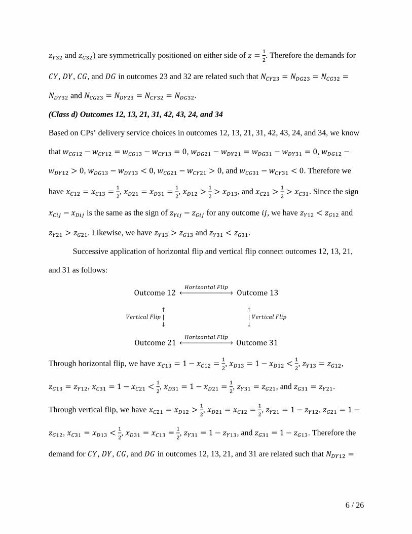
Successive application of horizontal flip and vertical flip connect outcomes 12, 13, 21,

and 31 as follows:

Outcome 12 𝐻𝐻𝐻𝐻𝐻𝐻𝐶𝐶𝐻𝐻𝐻𝐻𝐻𝐻𝑡𝑡𝐻𝐻𝐻𝐻 𝐹𝐹𝐻𝐻𝐶𝐶𝐹𝐹 �⎯⎯⎯⎯⎯⎯⎯⎯⎯⎯⎯⎯⎯� Outcome 13

𝑉𝑉𝑉𝑉𝑉𝑉𝑉𝑉𝑖𝑖𝑉𝑉𝑉𝑉𝑉𝑉 𝐹𝐹𝑉𝑉𝑖𝑖𝐹𝐹 ↑|↓

↑|↓

𝑉𝑉𝑉𝑉𝑉𝑉𝑉𝑉𝑖𝑖𝑉𝑉𝑉𝑉𝑉𝑉 𝐹𝐹𝑉𝑉𝑖𝑖𝐹𝐹

Outcome 21 𝐻𝐻𝐻𝐻𝐻𝐻𝐶𝐶𝐻𝐻𝐻𝐻𝐻𝐻𝑡𝑡𝐻𝐻𝐻𝐻 𝐹𝐹𝐻𝐻𝐶𝐶𝐹𝐹 �⎯⎯⎯⎯⎯⎯⎯⎯⎯⎯⎯⎯⎯� Outcome 31

Through horizontal flip, we have 𝑥𝑥𝐶𝐶13 = 1 − 𝑥𝑥𝐶𝐶12 = 12, 𝑥𝑥𝐷𝐷13 = 1 − 𝑥𝑥𝐷𝐷12 < 1

2, 𝑧𝑧𝑌𝑌13 = 𝑧𝑧𝐺𝐺12,

𝑧𝑧𝐺𝐺13 = 𝑧𝑧𝑌𝑌12, 𝑥𝑥𝐶𝐶31 = 1 − 𝑥𝑥𝐶𝐶21 < 12, 𝑥𝑥𝐷𝐷31 = 1 − 𝑥𝑥𝐷𝐷21 = 1

2, 𝑧𝑧𝑌𝑌31 = 𝑧𝑧𝐺𝐺21, and 𝑧𝑧𝐺𝐺31 = 𝑧𝑧𝑌𝑌21.

Through vertical flip, we have 𝑥𝑥𝐶𝐶21 = 𝑥𝑥𝐷𝐷12 > 12, 𝑥𝑥𝐷𝐷21 = 𝑥𝑥𝐶𝐶12 = 1

2, 𝑧𝑧𝑌𝑌21 = 1 − 𝑧𝑧𝑌𝑌12, 𝑧𝑧𝐺𝐺21 = 1 −

𝑧𝑧𝐺𝐺12, 𝑥𝑥𝐶𝐶31 = 𝑥𝑥𝐷𝐷13 < 12, 𝑥𝑥𝐷𝐷31 = 𝑥𝑥𝐶𝐶13 = 1

2, 𝑧𝑧𝑌𝑌31 = 1 − 𝑧𝑧𝑌𝑌13, and 𝑧𝑧𝐺𝐺31 = 1 − 𝑧𝑧𝐺𝐺13. Therefore the

demand for 𝐶𝐶𝐶𝐶, 𝐷𝐷𝐶𝐶, 𝐶𝐶𝐶𝐶, and 𝐷𝐷𝐶𝐶 in outcomes 12, 13, 21, and 31 are related such that 𝑁𝑁𝐷𝐷𝑌𝑌12 =

6 / 26

𝑁𝑁𝐷𝐷𝐺𝐺13 = 𝑁𝑁𝐶𝐶𝐺𝐺31 = 𝑁𝑁𝐶𝐶𝑌𝑌21, 𝑁𝑁𝐷𝐷𝐺𝐺12 = 𝑁𝑁𝐷𝐷𝑌𝑌13 = 𝑁𝑁𝐶𝐶𝑌𝑌31 = 𝑁𝑁𝐶𝐶𝐺𝐺21, 𝑁𝑁𝐶𝐶𝐺𝐺12 = 𝑁𝑁𝐶𝐶𝑌𝑌13 = 𝑁𝑁𝐷𝐷𝑌𝑌31 = 𝑁𝑁𝐷𝐷𝐺𝐺21,

and 𝑁𝑁𝐶𝐶𝑌𝑌12 = 𝑁𝑁𝐶𝐶𝐺𝐺13 = 𝑁𝑁𝐷𝐷𝐺𝐺31 = 𝑁𝑁𝐷𝐷𝑌𝑌21.

The demand analysis for outcomes 42, 43, 24, and 34 is the same as that in outcomes 12,

13, 21, and 31 since both CPs receive the same queuing priority when they both pay for

preferential delivery. Therefore, the demand for 𝐶𝐶𝐶𝐶, 𝐷𝐷𝐶𝐶, 𝐶𝐶𝐶𝐶, and 𝐷𝐷𝐶𝐶 in outcomes 42, 43, 24,

and 34 are related such that 𝑁𝑁𝐷𝐷𝑌𝑌42 = 𝑁𝑁𝐷𝐷𝐺𝐺43 = 𝑁𝑁𝐶𝐶𝐺𝐺34 = 𝑁𝑁𝐶𝐶𝑌𝑌24, 𝑁𝑁𝐷𝐷𝐺𝐺42 = 𝑁𝑁𝐷𝐷𝑌𝑌43 = 𝑁𝑁𝐶𝐶𝑌𝑌34 = 𝑁𝑁𝐶𝐶𝐺𝐺24,

𝑁𝑁𝐶𝐶𝐺𝐺42 = 𝑁𝑁𝐶𝐶𝑌𝑌43 = 𝑁𝑁𝐷𝐷𝑌𝑌34 = 𝑁𝑁𝐷𝐷𝐺𝐺24, and 𝑁𝑁𝐶𝐶𝑌𝑌42 = 𝑁𝑁𝐶𝐶𝐺𝐺43 = 𝑁𝑁𝐷𝐷𝐺𝐺34 = 𝑁𝑁𝐷𝐷𝑌𝑌24.

If 𝐶𝐶 and 𝐶𝐶 make identical decisions (1 or 4) on any ISP (𝐶𝐶 or 𝐷𝐷), consumers on that ISP

will receive the same queuing priority. For example, under outcomes 13 and 43, indifferent

customers of all four ISP-CP combinations are the same, which leads to identical demand

distribution for 𝐶𝐶𝐶𝐶, 𝐷𝐷𝐶𝐶, 𝐶𝐶𝐶𝐶, and 𝐷𝐷𝐶𝐶. That is 𝑁𝑁𝐶𝐶𝑌𝑌13 = 𝑁𝑁𝐶𝐶𝑌𝑌43, 𝑁𝑁𝐷𝐷𝑌𝑌13 = 𝑁𝑁𝐷𝐷𝑌𝑌43, 𝑁𝑁𝐶𝐶𝐺𝐺13 = 𝑁𝑁𝐶𝐶𝐺𝐺43,

and 𝑁𝑁𝐷𝐷𝐺𝐺13 = 𝑁𝑁𝐷𝐷𝐺𝐺43. By the same arguments above, we obtain the pairings with identical demand

distribution for 𝐶𝐶𝐶𝐶, 𝐷𝐷𝐶𝐶, 𝐶𝐶𝐶𝐶, and 𝐷𝐷𝐶𝐶: outcomes 12 and 42, outcomes 21 and 24, and outcomes

31 and 34.

Summarizing the above analysis, we conclude that the 16 outcomes can be grouped into

four classes invariant under horizontal and vertical flips with similar consumer demand patterns.

Proof of Lemma 2

We derive the ISPs’ equilibrium pricing strategies and the corresponding equilibrium outcomes

in the packet discrimination regime in the following steps: step 1, prove that any outcome

involving only 𝐶𝐶 pays on an ISP cannot be an equilibrium; step 2, derive properties of the

equilibrium fixed fee 𝐹𝐹; step 3, eliminate dominated outcomes; step 4, solve for the equilibrium

fixed fee 𝐹𝐹 and preferential delivery fee 𝐹𝐹 for the candidate outcomes; step 5, compare the

candidate outcomes and derive equilibrium outcomes.

7 / 26

Step 1: Prove that any outcome involving only 𝒀𝒀 pays on an ISP cannot be an equilibrium

In step 1, we show that there is no feasible 𝐹𝐹 for any outcome involving only 𝐶𝐶 pays on an ISP.

Therefore such outcomes (12, 21, 42, 24, 23, 32, and 22) cannot be an equilibrium. Since some

outcomes are infeasible for similar reasons, we group them together.

Outcomes 12 and 21

Here we focus on showing that there is no feasible 𝐹𝐹 for outcome 12, as the analysis for outcome

21 is similar. For outcomes 12 to be feasible, all the CPs’ incentive compatibility constraints

need to be satisfied: (1) 𝜋𝜋𝑌𝑌12 − 𝜋𝜋𝑌𝑌22 ≥ 0; (2) 𝜋𝜋𝑌𝑌12 − 𝜋𝜋𝑌𝑌11 ≥ 0; (3) 𝜋𝜋𝑌𝑌12 − 𝜋𝜋𝑌𝑌21 ≥ 0;

(4) 𝜋𝜋𝐺𝐺12 − 𝜋𝜋𝐺𝐺31 ≥ 0; (5) 𝜋𝜋𝐺𝐺12 − 𝜋𝜋𝐺𝐺14 ≥ 0; and (6) 𝜋𝜋𝐺𝐺12 − 𝜋𝜋𝐺𝐺34 ≥ 0.

Inequality (2) is −𝑁𝑁𝐷𝐷𝑌𝑌12𝐹𝐹 + (𝑁𝑁𝐶𝐶𝑌𝑌12 − 𝑁𝑁𝐶𝐶𝑌𝑌11 − 𝑁𝑁𝐷𝐷𝑌𝑌11 + 𝑁𝑁𝐷𝐷𝑌𝑌12)𝑉𝑉𝑌𝑌 ≥ 0. Since 𝑁𝑁𝐶𝐶𝑌𝑌12 +

𝑁𝑁𝐷𝐷𝑌𝑌12 > 12 and 𝑁𝑁𝐶𝐶𝑌𝑌11 + 𝑁𝑁𝐷𝐷𝑌𝑌11 = 1

2, inequality (2) can be reduced to 𝐹𝐹 ≤ (𝑁𝑁𝐶𝐶𝐶𝐶12+𝑁𝑁𝐷𝐷𝐶𝐶12−1 2⁄ )𝐻𝐻𝐶𝐶

𝑁𝑁𝐷𝐷𝐶𝐶12.

Inequality (5) is 𝑁𝑁𝐷𝐷𝐺𝐺14𝐹𝐹 + (𝑁𝑁𝐶𝐶𝐺𝐺12 − 𝑁𝑁𝐶𝐶𝐺𝐺14 + 𝑁𝑁𝐷𝐷𝐺𝐺12 − 𝑁𝑁𝐷𝐷𝐺𝐺14)𝑉𝑉𝐺𝐺 ≥ 0. Since 𝑁𝑁𝐷𝐷𝐺𝐺14 = 14,

𝑁𝑁𝐶𝐶𝐺𝐺14 + 𝑁𝑁𝐷𝐷𝐺𝐺14 = 12, and 𝑁𝑁𝐶𝐶𝐺𝐺12 + 𝑁𝑁𝐷𝐷𝐺𝐺12 < 1

2, inequality (5) can be reduced to 𝐹𝐹 ≥

(1 2⁄ −𝑁𝑁𝐶𝐶𝐶𝐶12−𝑁𝑁𝐷𝐷𝐶𝐶12)𝐻𝐻𝐶𝐶1 4⁄

.

We know that 12− 𝑁𝑁𝐶𝐶𝐺𝐺12 − 𝑁𝑁𝐷𝐷𝐺𝐺12 = 𝑁𝑁𝐶𝐶𝑌𝑌12 + 𝑁𝑁𝐷𝐷𝑌𝑌12 −

12, 𝑁𝑁𝐷𝐷𝑌𝑌12 > 1

4, and 𝑉𝑉𝐺𝐺 ≥ 𝑉𝑉𝑌𝑌 . Thus

we have (𝑁𝑁𝐶𝐶𝐶𝐶12+𝑁𝑁𝐷𝐷𝐶𝐶12−1 2⁄ )𝐻𝐻𝐶𝐶𝑁𝑁𝐷𝐷𝐶𝐶12

< (1 2⁄ −𝑁𝑁𝐶𝐶𝐶𝐶12−𝑁𝑁𝐷𝐷𝐶𝐶12)𝐻𝐻𝐶𝐶1 4⁄

. Therefore (2) and (5) are inconsistent.

Hence there is no solution for p that satisfies all incentive compatibility constraints for outcome

12.

8 / 26

Outcomes 42 and 24

Outcomes 24 and 42 are infeasible for similar reasons. Outcome 24 is not feasible since the

following incentive compatibility constraints are inconsistent: (1) 𝜋𝜋𝑌𝑌24 − 𝜋𝜋𝑌𝑌13 ≥ 0 and

(2) 𝜋𝜋𝐺𝐺24 − 𝜋𝜋𝐺𝐺44 ≥ 0.

Inequality (1) can be reduced to 𝐹𝐹 ≤ (𝑁𝑁𝐶𝐶𝐶𝐶24+𝑁𝑁𝐷𝐷𝐶𝐶24−𝑁𝑁𝐶𝐶𝐶𝐶13−𝑁𝑁𝐷𝐷𝐶𝐶13)𝐻𝐻𝐶𝐶(𝑁𝑁𝐶𝐶𝐶𝐶24+𝑁𝑁𝐷𝐷𝐶𝐶24) . Note that we have

𝑁𝑁𝐶𝐶𝑌𝑌24 + 𝑁𝑁𝐷𝐷𝑌𝑌24 − 𝑁𝑁𝐶𝐶𝑌𝑌13 − 𝑁𝑁𝐷𝐷𝑌𝑌13 = 𝑁𝑁𝐶𝐶𝑌𝑌24 + 𝑁𝑁𝐷𝐷𝑌𝑌24 −12

+ 12− 𝑁𝑁𝐶𝐶𝑌𝑌13 − 𝑁𝑁𝐷𝐷𝑌𝑌13 . Since 𝑁𝑁𝐶𝐶𝑌𝑌24 +

𝑁𝑁𝐷𝐷𝑌𝑌24 −12

= 12− 𝑁𝑁𝐶𝐶𝑌𝑌13 − 𝑁𝑁𝐷𝐷𝑌𝑌13 , we have 𝑁𝑁𝐶𝐶𝑌𝑌24 + 𝑁𝑁𝐷𝐷𝑌𝑌24 − 𝑁𝑁𝐶𝐶𝑌𝑌13 − 𝑁𝑁𝐷𝐷𝑌𝑌13 = 2 �𝑁𝑁𝐶𝐶𝑌𝑌24 +

𝑁𝑁𝐷𝐷𝑌𝑌24 −12� = 2 �1

2− 𝑁𝑁𝐶𝐶𝐺𝐺24 − 𝑁𝑁𝐷𝐷𝐺𝐺24� . Thus inequality (1) can be simplified to 𝐹𝐹 ≤

(1 2⁄ −𝑁𝑁𝐶𝐶𝐶𝐶24−𝑁𝑁𝐷𝐷𝐶𝐶24)𝐻𝐻𝐶𝐶(𝑁𝑁𝐶𝐶𝐶𝐶24+𝑁𝑁𝐷𝐷𝐶𝐶24) 2⁄

.

Inequality (2) can be reduced to 𝐹𝐹 ≥ (1 2⁄ −𝑁𝑁𝐶𝐶𝐶𝐶24−𝑁𝑁𝐷𝐷𝐶𝐶24)𝐻𝐻𝐶𝐶(1 2⁄ − 𝑁𝑁𝐷𝐷𝐶𝐶24) . Note that we have 𝑁𝑁𝐶𝐶𝑌𝑌24 +

𝑁𝑁𝐷𝐷𝑌𝑌24 + 𝑁𝑁𝐶𝐶𝐺𝐺24 + 𝑁𝑁𝐷𝐷𝐺𝐺24 = 1 . But 𝑁𝑁𝐶𝐶𝐺𝐺24 < 𝑁𝑁𝐷𝐷𝐺𝐺24 . Thus we have 𝑁𝑁𝐶𝐶𝐶𝐶24+𝑁𝑁𝐷𝐷𝐶𝐶242

> 12− 𝑁𝑁𝐷𝐷𝐺𝐺24 .

Therefore 𝐹𝐹 ≥ (1 2⁄ −𝑁𝑁𝐶𝐶𝐶𝐶24−𝑁𝑁𝐷𝐷𝐶𝐶24)𝐻𝐻𝐶𝐶(1 2⁄ − 𝑁𝑁𝐷𝐷𝐶𝐶24) > (1 2⁄ −𝑁𝑁𝐶𝐶𝐶𝐶24−𝑁𝑁𝐷𝐷𝐶𝐶24)𝐻𝐻𝐶𝐶

(𝑁𝑁𝐶𝐶𝐶𝐶24+𝑁𝑁𝐷𝐷𝐶𝐶24) 2⁄.

In addition, we know 𝑉𝑉𝐺𝐺 ≥ 𝑉𝑉𝑌𝑌 . Thus we have (1 2⁄ −𝑁𝑁𝐶𝐶𝐶𝐶24−𝑁𝑁𝐷𝐷𝐶𝐶24)𝐻𝐻𝐶𝐶(1 2⁄ − 𝑁𝑁𝐷𝐷𝐶𝐶24) >

(1 2⁄ −𝑁𝑁𝐶𝐶𝐶𝐶24−𝑁𝑁𝐷𝐷𝐶𝐶24)𝐻𝐻𝐶𝐶(𝑁𝑁𝐶𝐶𝐶𝐶24+𝑁𝑁𝐷𝐷𝐶𝐶24) 2⁄

≥ (1 2⁄ −𝑁𝑁𝐶𝐶𝐶𝐶24−𝑁𝑁𝐷𝐷𝐶𝐶24)𝐻𝐻𝐶𝐶(𝑁𝑁𝐶𝐶𝐶𝐶24+𝑁𝑁𝐷𝐷𝐶𝐶24) 2⁄

. Therefore inequalities (1) and (2) are inconsistent.

Hence outcome 24 is infeasible.

Outcomes 23 and 32

Outcomes 23 and 32 are infeasible for similar reasons. Outcome 23 is feasible provided 𝜋𝜋𝑌𝑌23 −

𝜋𝜋𝑌𝑌14 ≥ 0, i.e., �𝑁𝑁𝐶𝐶𝐺𝐺23 −14� 𝐹𝐹 + �1

2− 𝑁𝑁𝐶𝐶𝐺𝐺32 − 𝑁𝑁𝐶𝐶𝐺𝐺23� 𝑉𝑉𝑌𝑌 ≥ 0. Note that 𝑁𝑁𝐶𝐶𝐺𝐺23 + 𝑁𝑁𝐶𝐶𝑌𝑌23 = 1

2 and

𝑁𝑁𝐶𝐶𝑌𝑌23 = 𝑁𝑁𝐶𝐶𝐺𝐺32. Thus we have 𝑁𝑁𝐶𝐶𝐺𝐺23 + 𝑁𝑁𝐶𝐶𝐺𝐺32 = 12. This gives �𝑁𝑁𝐶𝐶𝐺𝐺23 −

14� 𝐹𝐹 ≥ 0. Since 𝑁𝑁𝐶𝐶𝐺𝐺23 <

9 / 26

14, we have 𝐹𝐹 ≤ 0. Hence there is no positive solution for 𝐹𝐹 and therefore outcome 23 is not

feasible.

Outcome 22

Outcome 22 is not feasible since the following incentive compatibility constraints are

inconsistent: (1) 𝜋𝜋𝑌𝑌22 − 𝜋𝜋𝑌𝑌11 ≥ 0 and (2) 𝜋𝜋𝐺𝐺22 − 𝜋𝜋𝐺𝐺44 ≥ 0.

Inequality (1) is �𝑁𝑁𝐶𝐶𝐺𝐺22 − 𝑁𝑁𝐶𝐶𝐺𝐺33 −12� 𝐹𝐹 + (𝑁𝑁𝐶𝐶𝐺𝐺33 − 𝑁𝑁𝐶𝐶𝐺𝐺22)𝑉𝑉𝑌𝑌 ≥ 0. Note that 𝑁𝑁𝐶𝐶𝐺𝐺22 +

𝑁𝑁𝐶𝐶𝑌𝑌22 = 12. Thus we have �𝑁𝑁𝐶𝐶𝐺𝐺22 − 𝑁𝑁𝐶𝐶𝐺𝐺33 −

12� = −𝑁𝑁𝐶𝐶𝐺𝐺33 − 𝑁𝑁𝐶𝐶𝑌𝑌22 = −2𝑁𝑁𝐶𝐶𝐺𝐺33 < 0. Therefore

inequality (1) can be reduced to 𝐹𝐹 ≤ �12− 𝑁𝑁𝐶𝐶𝐶𝐶22

2𝑁𝑁𝐶𝐶𝐶𝐶33� 𝑉𝑉𝑌𝑌. Inequality (2) can be reduced to 𝐹𝐹 ≥

(1 − 4𝑁𝑁𝐶𝐶𝐺𝐺22)𝑉𝑉𝐺𝐺.

Recall that 𝑁𝑁𝐶𝐶𝐺𝐺22 = 𝑁𝑁𝐶𝐶𝑌𝑌33, 𝑁𝑁𝐶𝐶𝑌𝑌22 = 𝑁𝑁𝐶𝐶𝐺𝐺33, and 𝑁𝑁𝐶𝐶𝑌𝑌33 + 𝑁𝑁𝐶𝐶𝐺𝐺33 = 12. Thus inequality (1)

may be re-written as 𝐹𝐹 ≤ �1 − 14𝑁𝑁𝐶𝐶𝐶𝐶33

� 𝑉𝑉𝑌𝑌 and inequality (2) may be re-written as 𝐹𝐹 ≥

4𝑁𝑁𝐶𝐶𝐺𝐺33 �1 − 14𝑁𝑁𝐶𝐶𝐶𝐶33

� 𝑉𝑉𝐺𝐺. Since 𝑉𝑉𝑌𝑌 ≤ 𝑉𝑉𝐺𝐺 and 4𝑁𝑁𝐶𝐶𝐺𝐺33 > 1, inequality (1) implies that 𝐹𝐹 ≤

�1 − 14𝑁𝑁𝐶𝐶𝐶𝐶33

� 𝑉𝑉𝑌𝑌 < 𝑉𝑉𝐺𝐺 but inequality (2) implies that 𝐹𝐹 ≥ 4𝑁𝑁𝐶𝐶𝐺𝐺33 �1 − 14𝑁𝑁𝐶𝐶𝐶𝐶33

� 𝑉𝑉𝐺𝐺 > 𝑉𝑉𝐺𝐺. Therefore

inequalities (1) and (2) are inconsistent and there is no feasible 𝐹𝐹 for outcome 22.

In summary, outcomes 12, 21, 42, 24, 23, 32, and 22 cannot be an equilibrium.

Step 2: Derive properties of the equilibrium fixed fee 𝑭𝑭

In step 2, we derive properties of the equilibrium fixed fee 𝐹𝐹. Here we first discuss some

properties for all 16 outcomes and thus the subscript 𝑖𝑖𝑖𝑖 is omitted in this discussion. Under the

assumption of full market coverage, the profit maximizing fixed fee 𝐹𝐹 is such that the consumers

10 / 26

of all four ISP-CP combinations (𝐶𝐶𝐶𝐶, 𝐷𝐷𝐶𝐶, 𝐶𝐶𝐶𝐶, and 𝐷𝐷𝐶𝐶) with the lowest net utility will get zero

net utility.

We now define the global utility function 𝑈𝑈(𝑥𝑥, 𝑧𝑧) for the entire market [0,1] × [0,1]. First

recall the definition of the demand distribution of each ISP-CP combinations characterized by

the utility functions.

𝑅𝑅𝐶𝐶𝑌𝑌 = {(𝑥𝑥, 𝑧𝑧) ∈ [0,1] × [0,1]; 𝑢𝑢𝐶𝐶𝑌𝑌(𝑥𝑥, 𝑧𝑧) ≥ max{𝑢𝑢𝐶𝐶𝐺𝐺(𝑥𝑥, 𝑧𝑧),𝑢𝑢𝐷𝐷𝑌𝑌(𝑥𝑥, 𝑧𝑧),𝑢𝑢𝐷𝐷𝐺𝐺(𝑥𝑥, 𝑧𝑧) } }

𝑅𝑅𝐷𝐷𝑌𝑌 = {(𝑥𝑥, 𝑧𝑧) ∈ [0,1] × [0,1]; 𝑢𝑢𝐷𝐷𝑌𝑌(𝑥𝑥, 𝑧𝑧) ≥ max{𝑢𝑢𝐷𝐷𝐺𝐺(𝑥𝑥, 𝑧𝑧),𝑢𝑢𝐶𝐶𝑌𝑌(𝑥𝑥, 𝑧𝑧),𝑢𝑢𝐶𝐶𝐺𝐺(𝑥𝑥, 𝑧𝑧)} }

𝑅𝑅𝐶𝐶𝐺𝐺 = {(𝑥𝑥, 𝑧𝑧) ∈ [0,1] × [0,1]; 𝑢𝑢𝐶𝐶𝐺𝐺(𝑥𝑥, 𝑧𝑧) ≥ max{𝑢𝑢𝐶𝐶𝑌𝑌(𝑥𝑥, 𝑧𝑧),𝑢𝑢𝐷𝐷𝐺𝐺(𝑥𝑥, 𝑧𝑧),𝑢𝑢𝐷𝐷𝑌𝑌(𝑥𝑥, 𝑧𝑧)} }

𝑅𝑅𝐷𝐷𝐺𝐺 = {(𝑥𝑥, 𝑧𝑧) ∈ [0,1] × [0,1]; 𝑢𝑢𝐷𝐷𝐺𝐺(𝑥𝑥, 𝑧𝑧) ≥ max{𝑢𝑢𝐷𝐷𝑌𝑌(𝑥𝑥, 𝑧𝑧),𝑢𝑢𝐶𝐶𝐺𝐺(𝑥𝑥, 𝑧𝑧),𝑢𝑢𝐶𝐶𝑌𝑌(𝑥𝑥, 𝑧𝑧)} }

Note that each of the following inequalities reduces to regions on [0,1] × [0,1] dictated by the

indifference customers between mutual pairs of ISP-CP combinations:

𝑢𝑢𝐶𝐶𝐺𝐺(𝑥𝑥, 𝑧𝑧) − 𝑢𝑢𝐶𝐶𝑌𝑌(𝑥𝑥, 𝑧𝑧) ≥ 0 ⟺ 𝑥𝑥 ≥ 𝑥𝑥𝐶𝐶

𝑢𝑢𝐷𝐷𝐺𝐺(𝑥𝑥, 𝑧𝑧) − 𝑢𝑢𝐷𝐷𝑌𝑌(𝑥𝑥, 𝑧𝑧) ≥ 0 ⟺ 𝑥𝑥 ≥ 𝑥𝑥𝐷𝐷

𝑢𝑢𝐷𝐷𝑌𝑌(𝑥𝑥, 𝑧𝑧) − 𝑢𝑢𝐶𝐶𝑌𝑌(𝑥𝑥, 𝑧𝑧) ≥ 0 ⟺ 𝑧𝑧 ≥ 𝑧𝑧𝑌𝑌

𝑢𝑢𝐷𝐷𝐺𝐺(𝑥𝑥, 𝑧𝑧) − 𝑢𝑢𝐶𝐶𝐺𝐺(𝑥𝑥, 𝑧𝑧) ≥ 0 ⟺ 𝑧𝑧 ≥ 𝑧𝑧𝐺𝐺

𝑢𝑢𝐷𝐷𝐺𝐺(𝑥𝑥, 𝑧𝑧) − 𝑢𝑢𝐶𝐶𝑌𝑌(𝑥𝑥, 𝑧𝑧) ≥ 0 ⟺ 𝑧𝑧 ≥ 𝐿𝐿−(𝑥𝑥)

𝑢𝑢𝐷𝐷𝑌𝑌(𝑥𝑥, 𝑧𝑧) − 𝑢𝑢𝐶𝐶𝐺𝐺(𝑥𝑥, 𝑧𝑧) ≥ 0 ⟺ 𝑧𝑧 ≥ 𝐿𝐿+(𝑥𝑥)

Then the demand distributions can be written in terms of the indifference customers as follows:

𝑅𝑅𝐶𝐶𝑌𝑌 = {(𝑥𝑥, 𝑧𝑧) ∈ [0,1] × [0,1]; 𝑥𝑥 ≤ 𝑥𝑥𝐶𝐶 , 𝑧𝑧 ≤ 𝑧𝑧𝑌𝑌, 𝑧𝑧 ≤ 𝐿𝐿−(𝑥𝑥) }

𝑅𝑅𝐷𝐷𝑌𝑌 = {(𝑥𝑥, 𝑧𝑧) ∈ [0,1] × [0,1]; 𝑥𝑥 ≤ 𝑥𝑥𝐷𝐷 , 𝑧𝑧 ≥ 𝑧𝑧𝑌𝑌, 𝑧𝑧 ≥ 𝐿𝐿+(𝑥𝑥) }

𝑅𝑅𝐶𝐶𝐺𝐺 = {(𝑥𝑥, 𝑧𝑧) ∈ [0,1] × [0,1]; 𝑥𝑥 ≥ 𝑥𝑥𝐶𝐶 , 𝑧𝑧 ≤ 𝑧𝑧𝐺𝐺 , 𝑧𝑧 ≤ 𝐿𝐿+(𝑥𝑥) }

𝑅𝑅𝐷𝐷𝐺𝐺 = {(𝑥𝑥, 𝑧𝑧) ∈ [0,1] × [0,1]; 𝑥𝑥 ≥ 𝑥𝑥𝐷𝐷 , 𝑧𝑧 ≥ 𝑧𝑧𝐺𝐺 , 𝑧𝑧 ≥ 𝐿𝐿−(𝑥𝑥) }

11 / 26

Define the global utility function 𝑈𝑈(𝑥𝑥, 𝑧𝑧) over the entire market [0,1] × [0,1]:

𝑈𝑈(𝑥𝑥, 𝑧𝑧) =

⎩⎨

⎧𝑢𝑢𝐶𝐶𝑌𝑌(𝑥𝑥, 𝑧𝑧),𝑢𝑢𝐷𝐷𝑌𝑌(𝑥𝑥, 𝑧𝑧),

if (𝑥𝑥, 𝑧𝑧) ∈ 𝑅𝑅𝐶𝐶𝑌𝑌if (𝑥𝑥, 𝑧𝑧) ∈ 𝑅𝑅𝐷𝐷𝑌𝑌

𝑢𝑢𝐶𝐶𝐺𝐺(𝑥𝑥, 𝑧𝑧),𝑢𝑢𝐷𝐷𝐺𝐺(𝑥𝑥, 𝑧𝑧),

if (𝑥𝑥, 𝑧𝑧) ∈ 𝑅𝑅𝐶𝐶𝐺𝐺if (𝑥𝑥, 𝑧𝑧) ∈ 𝑅𝑅𝐷𝐷𝐺𝐺

By definition of the demand regions 𝑅𝑅𝐶𝐶𝑌𝑌, 𝑅𝑅𝐷𝐷𝑌𝑌, 𝑅𝑅𝐶𝐶𝐺𝐺 , and 𝑅𝑅𝐷𝐷𝐺𝐺, the global utility function gives the

maximal utility value for the consumer (𝑥𝑥, 𝑧𝑧) according to its choice of ISP-CP combination. We

also note that 𝑈𝑈(𝑥𝑥, 𝑧𝑧) is a continuous function over the set [0,1] × [0,1]. Indeed, first note that

the functions 𝑢𝑢𝐶𝐶𝑌𝑌(𝑥𝑥, 𝑧𝑧), 𝑢𝑢𝐷𝐷𝑌𝑌(𝑥𝑥, 𝑧𝑧), 𝑢𝑢𝐶𝐶𝐺𝐺(𝑥𝑥, 𝑧𝑧), and 𝑢𝑢𝐷𝐷𝐺𝐺(𝑥𝑥, 𝑧𝑧) are linear functions in (𝑥𝑥, 𝑧𝑧) and

thus are all continuous. Since 𝑈𝑈(𝑥𝑥, 𝑧𝑧) is piecewise defined over demand regions 𝑅𝑅𝐶𝐶𝑌𝑌, 𝑅𝑅𝐷𝐷𝑌𝑌, 𝑅𝑅𝐶𝐶𝐺𝐺 ,

and 𝑅𝑅𝐷𝐷𝐺𝐺, we only need to check that 𝑈𝑈(𝑥𝑥, 𝑧𝑧) is continuous at each point on the boundaries

between mutual pairs of the demand regions 𝑅𝑅𝐶𝐶𝑌𝑌, 𝑅𝑅𝐷𝐷𝑌𝑌, 𝑅𝑅𝐶𝐶𝐺𝐺 , and 𝑅𝑅𝐷𝐷𝐺𝐺. We check each boundary:

• Between 𝑅𝑅𝐶𝐶𝑌𝑌 and 𝑅𝑅𝐷𝐷𝑌𝑌, the boundary is along the line 𝑧𝑧 = 𝑧𝑧𝑌𝑌 on which 𝑢𝑢𝐶𝐶𝑌𝑌 = 𝑢𝑢𝐷𝐷𝑌𝑌.

• Between 𝑅𝑅𝐶𝐶𝑌𝑌 and 𝑅𝑅𝐶𝐶𝐺𝐺 , the boundary is along the line 𝑥𝑥 = 𝑥𝑥𝐶𝐶 on which 𝑢𝑢𝐶𝐶𝑌𝑌 = 𝑢𝑢𝐶𝐶𝐺𝐺 .

• Between 𝑅𝑅𝐶𝐶𝑌𝑌 and 𝑅𝑅𝐷𝐷𝐺𝐺, the boundary is along the line 𝑧𝑧 = 𝐿𝐿−(𝑥𝑥) on which 𝑢𝑢𝐶𝐶𝑌𝑌 = 𝑢𝑢𝐷𝐷𝐺𝐺.

• Between 𝑅𝑅𝐷𝐷𝐺𝐺 and 𝑅𝑅𝐶𝐶𝐺𝐺 , the boundary is along the line 𝑧𝑧 = 𝑧𝑧𝐺𝐺 on which 𝑢𝑢𝐷𝐷𝐺𝐺 = 𝑢𝑢𝐶𝐶𝐺𝐺 .

• Between 𝑅𝑅𝐷𝐷𝐺𝐺 and 𝑅𝑅𝐷𝐷𝑌𝑌, the boundary is along the line 𝑥𝑥 = 𝑥𝑥𝐷𝐷 on which 𝑢𝑢𝐷𝐷𝐺𝐺 = 𝑢𝑢𝐷𝐷𝑌𝑌.

• Between 𝑅𝑅𝐷𝐷𝑌𝑌 and 𝑅𝑅𝐶𝐶𝐺𝐺 , the boundary is along the line 𝑧𝑧 = 𝐿𝐿+(𝑥𝑥) on which 𝑢𝑢𝐷𝐷𝑌𝑌 = 𝑢𝑢𝐶𝐶𝐺𝐺 .

Since corresponding utility functions all matches along the boundaries between mutual pairs of

the demand regions 𝑅𝑅𝐶𝐶𝑌𝑌, 𝑅𝑅𝐷𝐷𝑌𝑌, 𝑅𝑅𝐶𝐶𝐺𝐺 , and 𝑅𝑅𝐷𝐷𝐺𝐺, the global utility function 𝑈𝑈(𝑥𝑥, 𝑧𝑧) is continuous

over the entire set [0,1] × [0,1].

The global utility function 𝑈𝑈(𝑥𝑥, 𝑧𝑧) is a continuous function over the closed and bounded

set [0,1] × [0,1]. Therefore 𝑈𝑈(𝑥𝑥, 𝑧𝑧) attains its maximum and minimum at some points in the set

[0,1] × [0,1]. Under the assumption of full market coverage, the optimal fixed fees the ISPs

12 / 26

charge consumers are such that the minimum of 𝑈𝑈(𝑥𝑥, 𝑧𝑧) equal to zero. In other words, the

optimal fixed fee is the maximum fee such that all consumers get nonnegative utility.

Since 𝑈𝑈(𝑥𝑥, 𝑧𝑧) is piecewise defined by linear functions, it has no critical points in the

interior of each demand regions 𝑅𝑅𝐶𝐶𝑌𝑌, 𝑅𝑅𝐷𝐷𝑌𝑌, 𝑅𝑅𝐶𝐶𝐺𝐺 , and 𝑅𝑅𝐷𝐷𝐺𝐺. Therefore we only need to analyze the

value of 𝑈𝑈(𝑥𝑥, 𝑧𝑧) along each mutual boundaries to capture the minimum of 𝑈𝑈(𝑥𝑥, 𝑧𝑧). Before we

analyze the boundaries between 𝑅𝑅𝐶𝐶𝑌𝑌, 𝑅𝑅𝐷𝐷𝑌𝑌, 𝑅𝑅𝐶𝐶𝐺𝐺 , and 𝑅𝑅𝐷𝐷𝐺𝐺, we recall that the demand distributions

split into the three geometric types (i) 𝑥𝑥𝐶𝐶 = 𝑥𝑥𝐷𝐷 and 𝑧𝑧𝑌𝑌 = 𝑧𝑧𝐺𝐺; (ii) 𝑥𝑥𝐶𝐶 < 𝑥𝑥𝐷𝐷 and 𝑧𝑧𝑌𝑌 < 𝑧𝑧𝐺𝐺; and (iii)

𝑥𝑥𝐶𝐶 > 𝑥𝑥𝐷𝐷 and 𝑧𝑧𝑌𝑌 > 𝑧𝑧𝐺𝐺 .

The feasible outcomes 11, 14, 41, 44, and 33 are of type (i), where the demand regions

are all rectangular in shape. The feasible outcomes 31 and 34 are of type (ii), which have exactly

two rectangles, and two pentagonal regions sharing a boundary along 𝑧𝑧 = 𝐿𝐿+(𝑥𝑥). And finally,

the feasible outcomes 13 and 43 are of type (iii), which have exactly two rectangles, and two

pentagonal regions sharing a boundary along 𝑧𝑧 = 𝐿𝐿−(𝑥𝑥).

We organize the analysis into two cases (A): 𝑥𝑥𝐶𝐶 ≤ 𝑥𝑥𝐷𝐷and 𝑧𝑧𝑌𝑌 ≤ 𝑧𝑧𝐺𝐺 and (B): 𝑥𝑥𝐶𝐶 ≥ 𝑥𝑥𝐷𝐷 and

𝑧𝑧𝑌𝑌 ≥ 𝑧𝑧𝐺𝐺 . Obviously, Cases (A) and (B) overlaps in those of type (i) here the diagonal boundary

on 𝑧𝑧 = 𝐿𝐿+(𝑥𝑥) or 𝑧𝑧 = 𝐿𝐿−(𝑥𝑥) collapses to the point of intersection of these lines.

Case (A): 𝒙𝒙𝑪𝑪 ≤ 𝒙𝒙𝑫𝑫 and 𝒛𝒛𝒀𝒀 ≤ 𝒛𝒛𝑮𝑮

There are five boundaries including a segment on 𝑧𝑧 = 𝐿𝐿+(𝑥𝑥).

(A1) Boundary between 𝑅𝑅𝐶𝐶𝑌𝑌 and 𝑅𝑅𝐷𝐷𝑌𝑌. This boundary is along the horizontal line 𝑧𝑧 = 𝑧𝑧𝑌𝑌

and is the line segment joining (0, 𝑧𝑧𝑌𝑌) and the point (𝑥𝑥𝐶𝐶 , 𝑧𝑧𝑌𝑌). Since 𝑢𝑢𝐶𝐶𝑌𝑌 = 𝑢𝑢𝐷𝐷𝑌𝑌 on this boundary,

along the boundary we may write for 0 ≤ 𝑥𝑥 ≤ 𝑥𝑥𝐶𝐶 , 𝑈𝑈(𝑥𝑥, 𝑧𝑧𝑌𝑌) = 𝑢𝑢𝐶𝐶𝑌𝑌(𝑥𝑥, 𝑧𝑧𝑌𝑌) = 𝑉𝑉 − 𝑉𝑉𝑥𝑥 − 𝑘𝑘𝑧𝑧𝑌𝑌 −

𝑑𝑑𝑑𝑑𝑤𝑤𝐶𝐶𝑌𝑌 − 𝐹𝐹𝐶𝐶, or 𝑈𝑈(𝑥𝑥, 𝑧𝑧𝑌𝑌) = 𝑢𝑢𝐷𝐷𝑌𝑌(𝑥𝑥, 𝑧𝑧𝑌𝑌) = 𝑉𝑉 − 𝑉𝑉𝑥𝑥 − 𝑘𝑘(1 − 𝑧𝑧𝑌𝑌) − 𝑑𝑑𝑑𝑑𝑤𝑤𝐷𝐷𝑌𝑌 − 𝐹𝐹𝐷𝐷. In either formula,

13 / 26

we see that on this boundary 𝑈𝑈(𝑥𝑥, 𝑧𝑧) is a decreasing function of 𝑥𝑥. Therefore 𝑈𝑈(𝑥𝑥, 𝑧𝑧) minimizes

at (𝑥𝑥𝐶𝐶 , 𝑧𝑧𝑌𝑌) on the boundary between 𝑅𝑅𝐶𝐶𝑌𝑌 and 𝑅𝑅𝐷𝐷𝑌𝑌.

(A2) Boundary between 𝑅𝑅𝐷𝐷𝐺𝐺 and 𝑅𝑅𝐶𝐶𝐺𝐺 . This boundary is along the horizontal line 𝑧𝑧 = 𝑧𝑧𝐺𝐺

and is the line segment joining (𝑥𝑥𝐷𝐷 , 𝑧𝑧𝐺𝐺) and the point (1, 𝑧𝑧𝐺𝐺). Since 𝑢𝑢𝐷𝐷𝐺𝐺 = 𝑢𝑢𝐶𝐶𝐺𝐺 on this boundary,

along the boundary we may write for 𝑥𝑥𝐷𝐷 ≤ 𝑥𝑥 ≤ 1, 𝑈𝑈(𝑥𝑥, 𝑧𝑧𝐺𝐺) = 𝑢𝑢𝐶𝐶𝐺𝐺(𝑥𝑥, 𝑧𝑧𝐺𝐺) = 𝑉𝑉 − 𝑉𝑉(1 − 𝑥𝑥) −

𝑘𝑘𝑧𝑧𝐺𝐺 − 𝑑𝑑𝑑𝑑𝑤𝑤𝐶𝐶𝐺𝐺 − 𝐹𝐹𝐶𝐶 , or 𝑈𝑈(𝑥𝑥, 𝑧𝑧𝐺𝐺) = 𝑢𝑢𝐷𝐷𝐺𝐺(𝑥𝑥, 𝑧𝑧𝐺𝐺) = 𝑉𝑉 − 𝑉𝑉(1 − 𝑥𝑥) − 𝑘𝑘(1 − 𝑧𝑧𝐺𝐺) − 𝑑𝑑𝑑𝑑𝑤𝑤𝐷𝐷𝐺𝐺 − 𝐹𝐹𝐷𝐷. In

either formula, we see that on this boundary 𝑈𝑈(𝑥𝑥, 𝑧𝑧) is a increasing function of 𝑥𝑥. Therefore

𝑈𝑈(𝑥𝑥, 𝑧𝑧) minimizes at (𝑥𝑥𝐷𝐷 , 𝑧𝑧𝐺𝐺) on the boundary between 𝑅𝑅𝐷𝐷𝐺𝐺 and 𝑅𝑅𝐶𝐶𝐺𝐺 .

(A3) Boundary between 𝑅𝑅𝐶𝐶𝑌𝑌 and 𝑅𝑅𝐶𝐶𝐺𝐺 . This boundary is along the vertical line 𝑥𝑥 = 𝑥𝑥𝐶𝐶 and

is the line segment joining (𝑥𝑥𝐶𝐶 , 0) and the point (𝑥𝑥𝐶𝐶 , 𝑧𝑧𝑌𝑌). Since 𝑢𝑢𝐶𝐶𝑌𝑌 = 𝑢𝑢𝐶𝐶𝐺𝐺 on this boundary,

along the boundary we may write for 0 ≤ 𝑧𝑧 ≤ 𝑧𝑧𝑌𝑌, 𝑈𝑈(𝑥𝑥𝐶𝐶 , 𝑧𝑧) = 𝑢𝑢𝐶𝐶𝑌𝑌(𝑥𝑥𝐶𝐶 , 𝑧𝑧) = 𝑉𝑉 − 𝑉𝑉𝑥𝑥𝐶𝐶 − 𝑘𝑘𝑧𝑧 −

𝑑𝑑𝑑𝑑𝑤𝑤𝐶𝐶𝑌𝑌 − 𝐹𝐹𝐶𝐶, or 𝑈𝑈(𝑥𝑥𝐶𝐶 , 𝑧𝑧) = 𝑢𝑢𝐶𝐶𝐺𝐺(𝑥𝑥𝐶𝐶 , 𝑧𝑧) = 𝑉𝑉 − 𝑉𝑉(1 − 𝑥𝑥𝐶𝐶) − 𝑘𝑘𝑧𝑧 − 𝑑𝑑𝑑𝑑𝑤𝑤𝐶𝐶𝐺𝐺 − 𝐹𝐹𝐶𝐶 . In either formula,

we see that on this boundary 𝑈𝑈(𝑥𝑥, 𝑧𝑧) is a decreasing function of 𝑧𝑧. Therefore 𝑈𝑈(𝑥𝑥, 𝑧𝑧) minimizes

at (𝑥𝑥𝐶𝐶 , 𝑧𝑧𝑌𝑌) on the boundary between 𝑅𝑅𝐶𝐶𝑌𝑌 and 𝑅𝑅𝐶𝐶𝐺𝐺 .

(A4) Boundary between 𝑅𝑅𝐷𝐷𝐺𝐺 and 𝑅𝑅𝐷𝐷𝑌𝑌. This boundary is along the vertical line 𝑥𝑥 = 𝑥𝑥𝐷𝐷

and is the line segment joining (𝑥𝑥𝐷𝐷 , 𝑧𝑧𝐺𝐺) and the point (𝑥𝑥𝐷𝐷 , 1). Since 𝑢𝑢𝐶𝐶𝑌𝑌 = 𝑢𝑢𝐶𝐶𝐺𝐺 on this boundary,

along the boundary we may write for 𝑧𝑧𝐺𝐺 ≤ 𝑧𝑧 ≤ 1, 𝑈𝑈(𝑥𝑥𝐷𝐷 , 𝑧𝑧) = 𝑢𝑢𝐷𝐷𝑌𝑌(𝑥𝑥𝐷𝐷 , 𝑧𝑧) = 𝑉𝑉 − 𝑉𝑉𝑥𝑥𝐷𝐷 − 𝑘𝑘(1 −

𝑧𝑧) − 𝑑𝑑𝑑𝑑𝑤𝑤𝐷𝐷𝑌𝑌 − 𝐹𝐹𝐷𝐷, or 𝑈𝑈(𝑥𝑥𝐷𝐷 , 𝑧𝑧) = 𝑢𝑢𝐷𝐷𝐺𝐺(𝑥𝑥𝐷𝐷 , 𝑧𝑧) = 𝑉𝑉 − 𝑉𝑉(1 − 𝑥𝑥𝐷𝐷) − 𝑘𝑘(1 − 𝑧𝑧) − 𝑑𝑑𝑑𝑑𝑤𝑤𝐷𝐷𝐺𝐺 − 𝐹𝐹𝐷𝐷. In

either formula, we see that on this boundary 𝑈𝑈(𝑥𝑥, 𝑧𝑧) is a increasing function of 𝑧𝑧. Therefore

𝑈𝑈(𝑥𝑥, 𝑧𝑧) minimizes at (𝑥𝑥𝐷𝐷 , 𝑧𝑧𝐺𝐺) on the boundary between 𝑅𝑅𝐷𝐷𝐺𝐺 and 𝑅𝑅𝐷𝐷𝑌𝑌.

(A5) Boundary between 𝑅𝑅𝐶𝐶𝐺𝐺 and 𝑅𝑅𝐷𝐷𝑌𝑌. This boundary is along the line 𝑧𝑧 = 𝐿𝐿+(𝑥𝑥) and is

the line segment joining (𝑥𝑥𝐶𝐶 , 𝑧𝑧𝑌𝑌) and the point (𝑥𝑥𝐷𝐷 , 𝑧𝑧𝐺𝐺). We parameterize the directed line

segment as follows: For 0 ≤ 𝑠𝑠 ≤ 1, 𝑥𝑥 = (1 − 𝑠𝑠)𝑥𝑥𝐶𝐶 + 𝑠𝑠𝑥𝑥𝐷𝐷 and 𝑧𝑧 = (1 − 𝑠𝑠)𝑧𝑧𝑌𝑌 + 𝑠𝑠𝑧𝑧𝐺𝐺 . On this

14 / 26

boundary the utility function 𝑈𝑈 is a function of the parameter 𝑠𝑠. Since 𝑢𝑢𝐶𝐶𝐺𝐺 = 𝑢𝑢𝐷𝐷𝑌𝑌 on this

boundary, along the boundary we may write for 0 ≤ 𝑠𝑠 ≤ 1, 𝑈𝑈(𝑠𝑠) = 𝑢𝑢𝐷𝐷𝑌𝑌((1− 𝑠𝑠)𝑥𝑥𝐶𝐶 + 𝑠𝑠𝑥𝑥𝐷𝐷 , (1 −

𝑠𝑠)𝑧𝑧𝑌𝑌 + 𝑠𝑠𝑧𝑧𝐺𝐺) = 𝑉𝑉 − 𝑉𝑉[(1 − 𝑠𝑠)𝑥𝑥𝐶𝐶 + 𝑠𝑠𝑥𝑥𝐷𝐷] − 𝑘𝑘[1 − (1 − 𝑠𝑠)𝑧𝑧𝑌𝑌 − 𝑠𝑠𝑧𝑧𝐺𝐺] − 𝑑𝑑𝑑𝑑𝑤𝑤𝐷𝐷𝑌𝑌 − 𝐹𝐹𝐷𝐷 = 𝑉𝑉 +

𝑠𝑠𝑉𝑉(𝑥𝑥𝐶𝐶 − 𝑥𝑥𝐷𝐷) − 𝑉𝑉𝑥𝑥𝐶𝐶 − 𝑘𝑘(1 − 𝑧𝑧𝑌𝑌) + 𝑠𝑠𝑘𝑘(𝑧𝑧𝐺𝐺 − 𝑧𝑧𝑌𝑌) − 𝑑𝑑𝑑𝑑𝑤𝑤𝐷𝐷𝑌𝑌 − 𝐹𝐹𝐷𝐷, or 𝑈𝑈(𝑠𝑠) = 𝑢𝑢𝐶𝐶𝐺𝐺((1− 𝑠𝑠)𝑥𝑥𝐶𝐶 +

𝑠𝑠𝑥𝑥𝐷𝐷 , (1 − 𝑠𝑠)𝑧𝑧𝑌𝑌 + 𝑠𝑠𝑧𝑧𝐺𝐺) = 𝑉𝑉(𝑑𝑑) − 𝑉𝑉[1 − (1 − 𝑠𝑠)𝑥𝑥𝐶𝐶 − 𝑠𝑠𝑥𝑥𝐷𝐷] − 𝑘𝑘[(1 − 𝑠𝑠)𝑧𝑧𝑌𝑌 + 𝑠𝑠𝑧𝑧𝐺𝐺] − 𝑑𝑑𝑑𝑑𝑤𝑤𝐶𝐶𝐺𝐺 −

𝐹𝐹𝐶𝐶 = 𝑉𝑉(𝑑𝑑) − 𝑉𝑉(1 − 𝑥𝑥𝐶𝐶) + 𝑠𝑠𝑉𝑉(𝑥𝑥𝐷𝐷 − 𝑥𝑥𝐶𝐶) − 𝑘𝑘𝑧𝑧𝑌𝑌 + 𝑠𝑠𝑘𝑘(𝑧𝑧𝑌𝑌 − 𝑧𝑧𝐺𝐺) − 𝑑𝑑𝑑𝑑𝑤𝑤𝐶𝐶𝐺𝐺 − 𝐹𝐹𝐶𝐶 . If 𝑥𝑥𝐷𝐷 = 𝑥𝑥𝐶𝐶 and

𝑧𝑧𝑌𝑌 = 𝑧𝑧𝐺𝐺 then 𝑈𝑈(𝑠𝑠) is a constant not dependent on 𝑠𝑠. However, in general we note that the slope

of 𝑧𝑧 = 𝐿𝐿+(𝑥𝑥) is given by 𝑡𝑡𝑘𝑘

= 𝐻𝐻𝐶𝐶−𝐻𝐻𝐶𝐶𝑥𝑥𝐷𝐷−𝑥𝑥𝐶𝐶

, i.e., 𝑘𝑘(𝑧𝑧𝐺𝐺 − 𝑧𝑧𝑌𝑌) = 𝑉𝑉(𝑥𝑥𝐷𝐷 − 𝑥𝑥𝐶𝐶). Thus the values of 𝑈𝑈(𝑠𝑠)

reduces to the constant: 𝑈𝑈(𝑠𝑠) = 𝑉𝑉 − 𝑉𝑉𝑥𝑥𝐶𝐶 − 𝑘𝑘(1 − 𝑧𝑧𝑌𝑌) − 𝑑𝑑𝑑𝑑𝑤𝑤𝐷𝐷𝑌𝑌 − 𝐹𝐹𝐷𝐷 or 𝑈𝑈(𝑠𝑠) = 𝑉𝑉 − 𝑉𝑉(1 −

𝑥𝑥𝐶𝐶) − 𝑘𝑘𝑧𝑧𝑌𝑌 − 𝑑𝑑𝑑𝑑𝑤𝑤𝐶𝐶𝐺𝐺 − 𝐹𝐹𝐶𝐶. From the analysis above, we could see that 𝑈𝑈(𝑥𝑥, 𝑧𝑧) minimizes on the

points along the boundary on the line 𝑧𝑧 = 𝐿𝐿+(𝑥𝑥). In particular, 𝑈𝑈(𝑥𝑥, 𝑧𝑧) minimizes at (𝑥𝑥𝐶𝐶 , 𝑧𝑧𝑌𝑌) or

(𝑥𝑥𝐷𝐷 , 𝑧𝑧𝐺𝐺) with the same value.

Case (B): 𝒙𝒙𝑪𝑪 ≥ 𝒙𝒙𝑫𝑫and 𝒛𝒛𝒀𝒀 ≥ 𝒛𝒛𝑮𝑮

There are five boundaries including a segment on 𝑧𝑧 = 𝐿𝐿−(𝑥𝑥).

(B1) Boundary between 𝑅𝑅𝐶𝐶𝑌𝑌 and 𝑅𝑅𝐷𝐷𝑌𝑌. This boundary is along the horizontal line 𝑧𝑧 = 𝑧𝑧𝑌𝑌

and is the line segment joining (0, 𝑧𝑧𝑌𝑌) and the point (𝑥𝑥𝐷𝐷 , 𝑧𝑧𝑌𝑌). Since 𝑢𝑢𝐶𝐶𝑌𝑌 = 𝑢𝑢𝐷𝐷𝑌𝑌 on this boundary,

along the boundary we may write for 0 ≤ 𝑥𝑥 ≤ 𝑥𝑥𝐷𝐷, 𝑈𝑈(𝑥𝑥, 𝑧𝑧𝑌𝑌) = 𝑢𝑢𝐶𝐶𝑌𝑌(𝑥𝑥, 𝑧𝑧𝑌𝑌) = 𝑉𝑉 − 𝑉𝑉𝑥𝑥 − 𝑘𝑘𝑧𝑧𝑌𝑌 −

𝑑𝑑𝑑𝑑𝑤𝑤𝐶𝐶𝑌𝑌 − 𝐹𝐹𝐶𝐶, or 𝑈𝑈(𝑥𝑥, 𝑧𝑧𝑌𝑌) = 𝑢𝑢𝐷𝐷𝑌𝑌(𝑥𝑥, 𝑧𝑧𝑌𝑌) = 𝑉𝑉 − 𝑉𝑉𝑥𝑥 − 𝑘𝑘(1 − 𝑧𝑧𝑌𝑌) − 𝑑𝑑𝑑𝑑𝑤𝑤𝐷𝐷𝑌𝑌 − 𝐹𝐹𝐷𝐷. In either formula,

we see that on this boundary 𝑈𝑈(𝑥𝑥, 𝑧𝑧) is a decreasing function of 𝑥𝑥. Therefore 𝑈𝑈(𝑥𝑥, 𝑧𝑧) minimizes

at (𝑥𝑥𝐷𝐷 , 𝑧𝑧𝑌𝑌) on the boundary between 𝑅𝑅𝐶𝐶𝑌𝑌 and 𝑅𝑅𝐷𝐷𝑌𝑌.

(B2) Boundary between 𝑅𝑅𝐷𝐷𝐺𝐺 and 𝑅𝑅𝐶𝐶𝐺𝐺 . This boundary is along the horizontal line 𝑧𝑧 = 𝑧𝑧𝐺𝐺

and is the line segment joining (𝑥𝑥𝐶𝐶 , 𝑧𝑧𝐺𝐺) and the point (1, 𝑧𝑧𝐺𝐺). Since 𝑢𝑢𝐷𝐷𝐺𝐺 = 𝑢𝑢𝐶𝐶𝐺𝐺 on this boundary,

15 / 26

along the boundary we may write for 𝑥𝑥𝐶𝐶 ≤ 𝑥𝑥 ≤ 1, 𝑈𝑈(𝑥𝑥, 𝑧𝑧𝐺𝐺) = 𝑢𝑢𝐶𝐶𝐺𝐺(𝑥𝑥, 𝑧𝑧𝐺𝐺) = 𝑉𝑉 − 𝑉𝑉(1 − 𝑥𝑥) −

𝑘𝑘𝑧𝑧𝐺𝐺 − 𝑑𝑑𝑑𝑑𝑤𝑤𝐶𝐶𝐺𝐺 − 𝐹𝐹𝐶𝐶 , or 𝑈𝑈(𝑥𝑥, 𝑧𝑧𝐺𝐺) = 𝑢𝑢𝐷𝐷𝐺𝐺(𝑥𝑥, 𝑧𝑧𝐺𝐺) = 𝑉𝑉 − 𝑉𝑉(1 − 𝑥𝑥) − 𝑘𝑘(1 − 𝑧𝑧𝐺𝐺) − 𝑑𝑑𝑑𝑑𝑤𝑤𝐷𝐷𝐺𝐺 − 𝐹𝐹𝐷𝐷. In

either formula, we see that on this boundary 𝑈𝑈(𝑥𝑥, 𝑧𝑧) is a increasing function of 𝑥𝑥. Therefore

𝑈𝑈(𝑥𝑥, 𝑧𝑧) minimizes at (𝑥𝑥𝐶𝐶 , 𝑧𝑧𝐺𝐺) on the boundary between 𝑅𝑅𝐷𝐷𝐺𝐺 and 𝑅𝑅𝐶𝐶𝐺𝐺 .

(B3) Boundary between 𝑅𝑅𝐶𝐶𝑌𝑌 and 𝑅𝑅𝐶𝐶𝐺𝐺 . This boundary is along the vertical line 𝑥𝑥 = 𝑥𝑥𝐶𝐶 and

is the line segment joining (𝑥𝑥𝐶𝐶 , 0) and the point (𝑥𝑥𝐶𝐶 , 𝑧𝑧𝐺𝐺). Since 𝑢𝑢𝐶𝐶𝑌𝑌 = 𝑢𝑢𝐶𝐶𝐺𝐺 on this boundary,

along the boundary we may write for 0 ≤ 𝑧𝑧 ≤ 𝑧𝑧𝐺𝐺 , 𝑈𝑈(𝑥𝑥𝐶𝐶 , 𝑧𝑧) = 𝑢𝑢𝐶𝐶𝑌𝑌(𝑥𝑥𝐶𝐶 , 𝑧𝑧) = 𝑉𝑉 − 𝑉𝑉𝑥𝑥𝐶𝐶 − 𝑘𝑘𝑧𝑧 −

𝑑𝑑𝑑𝑑𝑤𝑤𝐶𝐶𝑌𝑌 − 𝐹𝐹𝐶𝐶, or 𝑈𝑈(𝑥𝑥𝐶𝐶 , 𝑧𝑧) = 𝑢𝑢𝐶𝐶𝐺𝐺(𝑥𝑥𝐶𝐶 , 𝑧𝑧) = 𝑉𝑉 − 𝑉𝑉(1 − 𝑥𝑥𝐶𝐶) − 𝑘𝑘𝑧𝑧 − 𝑑𝑑𝑑𝑑𝑤𝑤𝐶𝐶𝐺𝐺 − 𝐹𝐹𝐶𝐶 . In either formula,

we see that on this boundary 𝑈𝑈(𝑥𝑥, 𝑧𝑧) is a decreasing function of 𝑧𝑧. Therefore 𝑈𝑈(𝑥𝑥, 𝑧𝑧) minimizes

at (𝑥𝑥𝐶𝐶 , 𝑧𝑧𝐺𝐺) on the boundary between 𝑅𝑅𝐶𝐶𝑌𝑌 and 𝑅𝑅𝐶𝐶𝐺𝐺 .

(B4) Boundary between 𝑅𝑅𝐷𝐷𝐺𝐺 and 𝑅𝑅𝐷𝐷𝑌𝑌. This boundary is along the vertical line 𝑥𝑥 = 𝑥𝑥𝐷𝐷

and is the line segment joining (𝑥𝑥𝐷𝐷 , 𝑧𝑧𝑌𝑌) and the point (𝑥𝑥𝐷𝐷 , 1). Since 𝑢𝑢𝐶𝐶𝑌𝑌 = 𝑢𝑢𝐶𝐶𝐺𝐺 on this boundary,

along the boundary we may write for 𝑧𝑧𝑌𝑌 ≤ 𝑧𝑧 ≤ 1, 𝑈𝑈(𝑥𝑥𝐷𝐷 , 𝑧𝑧) = 𝑢𝑢𝐷𝐷𝑌𝑌(𝑥𝑥𝐷𝐷 , 𝑧𝑧) = 𝑉𝑉 − 𝑉𝑉𝑥𝑥𝐷𝐷 − 𝑘𝑘(1 −

𝑧𝑧) − 𝑑𝑑𝑑𝑑𝑤𝑤𝐷𝐷𝑌𝑌 − 𝐹𝐹𝐷𝐷, or 𝑈𝑈(𝑥𝑥𝐷𝐷 , 𝑧𝑧) = 𝑢𝑢𝐷𝐷𝐺𝐺(𝑥𝑥𝐷𝐷 , 𝑧𝑧) = 𝑉𝑉 − 𝑉𝑉(1 − 𝑥𝑥𝐷𝐷) − 𝑘𝑘(1 − 𝑧𝑧) − 𝑑𝑑𝑑𝑑𝑤𝑤𝐷𝐷𝐺𝐺 − 𝐹𝐹𝐷𝐷. In

either formula, we see that on this boundary 𝑈𝑈(𝑥𝑥, 𝑧𝑧) is a increasing function of 𝑧𝑧. Therefore

𝑈𝑈(𝑥𝑥, 𝑧𝑧) minimizes at (𝑥𝑥𝐷𝐷 , 𝑧𝑧𝑌𝑌) on the boundary between 𝑅𝑅𝐷𝐷𝐺𝐺 and 𝑅𝑅𝐷𝐷𝑌𝑌.

(B5) Boundary between 𝑅𝑅𝐶𝐶𝑌𝑌 and 𝑅𝑅𝐷𝐷𝐺𝐺. This boundary is along the line 𝑧𝑧 = 𝐿𝐿−(𝑥𝑥) and is

the line segment joining (𝑥𝑥𝐷𝐷 , 𝑧𝑧𝑌𝑌) and the point (𝑥𝑥𝐶𝐶 , 𝑧𝑧𝐺𝐺). We parameterize the directed line

segment as follows: For 0 ≤ 𝑠𝑠 ≤ 1, 𝑥𝑥 = (1 − 𝑠𝑠)𝑥𝑥𝐷𝐷 + 𝑠𝑠𝑥𝑥𝐶𝐶 and 𝑧𝑧 = (1 − 𝑠𝑠)𝑧𝑧𝑌𝑌 + 𝑠𝑠𝑧𝑧𝐺𝐺 . On this

boundary the utility function 𝑈𝑈 is a function of the parameter 𝑠𝑠. Since 𝑢𝑢𝐶𝐶𝑌𝑌 = 𝑢𝑢𝐷𝐷𝐺𝐺 on this

boundary, along the boundary we may write for 0 ≤ 𝑠𝑠 ≤ 1, 𝑈𝑈(𝑠𝑠) = 𝑢𝑢𝐷𝐷𝐺𝐺((1 − 𝑠𝑠)𝑥𝑥𝐷𝐷 + 𝑠𝑠𝑥𝑥𝐶𝐶 , (1 −

𝑠𝑠)𝑧𝑧𝑌𝑌 + 𝑠𝑠𝑧𝑧𝐺𝐺) = 𝑉𝑉 − 𝑉𝑉[1 − (1 − 𝑠𝑠)𝑥𝑥𝐷𝐷 − 𝑠𝑠𝑥𝑥𝐶𝐶] − 𝑘𝑘[1 − (1 − 𝑠𝑠)𝑧𝑧𝑌𝑌 − 𝑠𝑠𝑧𝑧𝐺𝐺] − 𝑑𝑑𝑑𝑑𝑤𝑤𝐷𝐷𝐺𝐺 − 𝐹𝐹𝐷𝐷 = 𝑉𝑉 +

𝑠𝑠𝑉𝑉(𝑥𝑥𝐶𝐶 − 𝑥𝑥𝐷𝐷) − 𝑉𝑉(1 − 𝑥𝑥𝐷𝐷) − 𝑘𝑘(1 − 𝑧𝑧𝑌𝑌) + 𝑠𝑠𝑘𝑘(𝑧𝑧𝐺𝐺 − 𝑧𝑧𝑌𝑌) − 𝑑𝑑𝑑𝑑𝑤𝑤𝐷𝐷𝐺𝐺 − 𝐹𝐹𝐷𝐷, or 𝑈𝑈(𝑠𝑠) = 𝑢𝑢𝐶𝐶𝑌𝑌((1−

16 / 26

𝑠𝑠)𝑥𝑥𝐷𝐷 + 𝑠𝑠𝑥𝑥𝐶𝐶 , (1 − 𝑠𝑠)𝑧𝑧𝑌𝑌 + 𝑠𝑠𝑧𝑧𝐺𝐺) = 𝑉𝑉 − 𝑉𝑉[(1 − 𝑠𝑠)𝑥𝑥𝐷𝐷 + 𝑠𝑠𝑥𝑥𝐶𝐶] − 𝑘𝑘[(1 − 𝑠𝑠)𝑧𝑧𝑌𝑌 + 𝑠𝑠𝑧𝑧𝐺𝐺] − 𝑑𝑑𝑑𝑑𝑤𝑤𝐶𝐶𝑌𝑌 −

𝐹𝐹𝐶𝐶 = 𝑉𝑉 − 𝑉𝑉𝑥𝑥𝐷𝐷 + 𝑠𝑠𝑉𝑉(𝑥𝑥𝐷𝐷 − 𝑥𝑥𝐶𝐶) − 𝑘𝑘𝑧𝑧𝑌𝑌 + 𝑠𝑠𝑘𝑘(𝑧𝑧𝑌𝑌 − 𝑧𝑧𝐺𝐺) − 𝑑𝑑𝑑𝑑𝑤𝑤𝐶𝐶𝑌𝑌 − 𝐹𝐹𝐶𝐶 . If 𝑥𝑥𝐷𝐷 = 𝑥𝑥𝐶𝐶 and 𝑧𝑧𝑌𝑌 = 𝑧𝑧𝐺𝐺 then

𝑈𝑈(𝑠𝑠) is a constant not dependent on 𝑠𝑠. However, in general we note that the slope of 𝑧𝑧 = 𝐿𝐿−(𝑥𝑥)

is given by: − 𝑡𝑡𝑘𝑘

= 𝐻𝐻𝐶𝐶−𝐻𝐻𝐶𝐶𝑥𝑥𝐶𝐶−𝑥𝑥𝐷𝐷

, i.e., 𝑘𝑘(𝑧𝑧𝐺𝐺 − 𝑧𝑧𝑌𝑌) = 𝑉𝑉(𝑥𝑥𝐷𝐷 − 𝑥𝑥𝐶𝐶). Thus the values of 𝑈𝑈(𝑠𝑠) reduces to the

constant: 𝑈𝑈(𝑠𝑠) = 𝑉𝑉 − 𝑉𝑉(1 − 𝑥𝑥𝐷𝐷) − 𝑘𝑘(1 − 𝑧𝑧𝑌𝑌) − 𝑑𝑑𝑑𝑑𝑤𝑤𝐷𝐷𝐺𝐺 − 𝐹𝐹𝐷𝐷 or 𝑈𝑈(𝑠𝑠) = 𝑉𝑉 − 𝑉𝑉𝑥𝑥𝐷𝐷 − 𝑘𝑘𝑧𝑧𝑌𝑌 −

𝑑𝑑𝑑𝑑𝑤𝑤𝐶𝐶𝑌𝑌 − 𝐹𝐹𝐶𝐶. From the analysis above, we could see that 𝑈𝑈(𝑥𝑥, 𝑧𝑧) minimizes on the points along

the boundary on the line 𝑧𝑧 = 𝐿𝐿−(𝑥𝑥). In particular, 𝑈𝑈(𝑥𝑥, 𝑧𝑧) minimizes at (𝑥𝑥𝐷𝐷 , 𝑧𝑧𝑌𝑌) or (𝑥𝑥𝐶𝐶 , 𝑧𝑧𝐺𝐺) with

the same value.

Maximum Fees for Case A: The maximum fees occur when the minimum of the global

utility function is zero. Therefore from the formulas in (A5), the maximum fees are given by:

𝑉𝑉 − 𝑉𝑉𝑥𝑥𝐶𝐶 − 𝑘𝑘(1 − 𝑧𝑧𝑌𝑌) − 𝑑𝑑𝑑𝑑𝑤𝑤𝐷𝐷𝑌𝑌 − 𝐹𝐹𝐷𝐷 = 0 and 𝑉𝑉 − 𝑉𝑉(1 − 𝑥𝑥𝐶𝐶) − 𝑘𝑘𝑧𝑧𝑌𝑌 − 𝑑𝑑𝑑𝑑𝑤𝑤𝐶𝐶𝐺𝐺 − 𝐹𝐹𝐶𝐶 = 0. This

gives the maximum fees: 𝐹𝐹𝐶𝐶 = 𝑉𝑉 − 𝑉𝑉 �1 − 𝑥𝑥𝐶𝐶+𝑥𝑥𝐷𝐷2

� − 𝑘𝑘 �𝐻𝐻𝐶𝐶+𝐻𝐻𝐶𝐶2

� − 𝑑𝑑𝑑𝑑𝑤𝑤𝐶𝐶𝐺𝐺 and 𝐹𝐹𝐷𝐷 = 𝑉𝑉 −

𝑉𝑉 �𝑥𝑥𝐶𝐶+𝑥𝑥𝐷𝐷2

� − 𝑘𝑘 �1 − 𝐻𝐻𝐶𝐶+𝐻𝐻𝐶𝐶2

� − 𝑑𝑑𝑑𝑑𝑤𝑤𝐷𝐷𝑌𝑌.

Maximum Fees for Case B: The maximum fees occur when the minimum of the global

utility function is zero. Therefore from the formulas in (B5), the maximum fees are given by:

𝑉𝑉 − 𝑉𝑉(1 − 𝑥𝑥𝐷𝐷) − 𝑘𝑘(1 − 𝑧𝑧𝑌𝑌) − 𝑑𝑑𝑑𝑑𝑤𝑤𝐷𝐷𝐺𝐺 − 𝐹𝐹𝐷𝐷 = 0 and 𝑉𝑉 − 𝑉𝑉𝑥𝑥𝐷𝐷 − 𝑘𝑘𝑧𝑧𝑌𝑌 − 𝑑𝑑𝑑𝑑𝑤𝑤𝐶𝐶𝑌𝑌 − 𝐹𝐹𝐶𝐶 = 0. This

gives the maximum fees: 𝐹𝐹𝐶𝐶 = 𝑉𝑉 − 𝑉𝑉 �𝑥𝑥𝐶𝐶+𝑥𝑥𝐷𝐷2

� − 𝑘𝑘 �𝐻𝐻𝐶𝐶+𝐻𝐻𝐶𝐶2

� − 𝑑𝑑𝑑𝑑𝑤𝑤𝐶𝐶𝑌𝑌 and 𝐹𝐹𝐷𝐷 = 𝑉𝑉 − 𝑉𝑉 �1 −

𝑥𝑥𝐶𝐶+𝑥𝑥𝐷𝐷2

� − 𝑘𝑘 �1 − 𝐻𝐻𝐶𝐶+𝐻𝐻𝐶𝐶2

� − 𝑑𝑑𝑑𝑑𝑤𝑤𝐷𝐷𝐺𝐺.

We next solve for the optimal fixed fee for feasible outcomes in symmetric equilibrium

when 𝐹𝐹𝐶𝐶 = 𝐹𝐹𝐷𝐷 = 𝐹𝐹.

17 / 26

Optimal 𝐹𝐹 for outcomes 11, 14, 41, and 44: All waiting times are the same and 𝑥𝑥𝐶𝐶 =

𝑥𝑥𝐷𝐷 = 𝑧𝑧𝑌𝑌 = 𝑧𝑧𝐺𝐺 = 12. Using the formulas for maximum fees above, we get 𝐹𝐹11 = 𝐹𝐹14 = 𝐹𝐹41 =

𝐹𝐹44 = 𝑉𝑉 − 𝑡𝑡2− 𝑘𝑘

2− 𝑑𝑑𝑑𝑑

𝜇𝜇−𝑑𝑑 2⁄.

Optimal 𝐹𝐹 for outcome 33: In this outcome, 𝑧𝑧𝑌𝑌33 = 𝑧𝑧𝐺𝐺33 = 12 and 𝑥𝑥𝐷𝐷33 = 𝑥𝑥𝐶𝐶33 < 1

2. We

have four formulas for F which must be consistent. We verify that those in Case A and Case B

both reduces to the following formula for 𝐹𝐹: 𝐹𝐹33 = 𝑉𝑉 − 𝑉𝑉(1 − 𝑥𝑥𝐷𝐷33) − 𝑘𝑘2− 2𝑑𝑑𝑑𝑑

2𝜇𝜇−(1−𝑥𝑥𝐷𝐷33)𝑑𝑑.

Optimal 𝐹𝐹 for outcomes 13 and 43: These outcomes have the same demand distributions

and so the same indifferent customers and waiting times. We use the formulas for Case B for

these outcomes: 𝐹𝐹43 = 𝐹𝐹13 = 𝑉𝑉 − 𝑉𝑉(1 − 𝑥𝑥𝐷𝐷43) − 𝑘𝑘(1 − 𝑧𝑧𝑌𝑌43) − 𝑑𝑑𝑑𝑑𝜇𝜇−𝑁𝑁𝐷𝐷𝐶𝐶43𝑑𝑑

.

Optimal 𝐹𝐹 for outcomes 31 and 34: These outcomes have the same demand distributions

and so the same indifferent customers and waiting times. We use the formulas for Case A for

these outcomes: 𝐹𝐹34 = 𝐹𝐹31 = 𝑉𝑉 − 𝑉𝑉(1 − 𝑥𝑥𝐶𝐶34) − 𝑘𝑘𝑧𝑧𝑌𝑌34 −𝑑𝑑𝑑𝑑

𝜇𝜇−𝑁𝑁𝐶𝐶𝐶𝐶34𝑑𝑑.

Step 3: Eliminate dominated outcomes

From Step 1, we know that any outcome involving only 𝐶𝐶 pays on an ISP cannot be an

equilibrium. Therefore, outcomes 12, 21, 22, 23, 24, 32, and 42 can be eliminated from the

equilibrium analysis as shown in the following table.

Decisions of 𝐶𝐶 and 𝐶𝐶 on ISP 𝐷𝐷 1: Neither pays 𝐷𝐷

2: 𝐶𝐶 pays 𝐷𝐷 3: 𝐶𝐶 pays 𝐷𝐷 4: both pay 𝐷𝐷

Decisions of 𝐶𝐶 and 𝐶𝐶 on ISP 𝐶𝐶

1: Neither pays 𝐶𝐶

(𝜋𝜋𝐶𝐶11,𝜋𝜋𝐷𝐷11) (𝜋𝜋𝐶𝐶12,𝜋𝜋𝐷𝐷12) (𝜋𝜋𝐶𝐶13,𝜋𝜋𝐷𝐷13) (𝜋𝜋𝐶𝐶14,𝜋𝜋𝐷𝐷14)

2: 𝐶𝐶 pays 𝐶𝐶 (𝜋𝜋𝐶𝐶21,𝜋𝜋𝐷𝐷21) (𝜋𝜋𝐶𝐶22,𝜋𝜋𝐷𝐷22) (𝜋𝜋𝐶𝐶23,𝜋𝜋𝐷𝐷23) (𝜋𝜋𝐶𝐶24,𝜋𝜋𝐷𝐷24) 3: 𝐶𝐶 pays 𝐶𝐶 (𝜋𝜋𝐶𝐶31,𝜋𝜋𝐷𝐷11) (𝜋𝜋𝐶𝐶32,𝜋𝜋𝐷𝐷32) (𝜋𝜋𝐶𝐶33,𝜋𝜋𝐷𝐷33) (𝜋𝜋𝐶𝐶34,𝜋𝜋𝐷𝐷34) 4: both pay 𝐶𝐶 (𝜋𝜋𝐶𝐶41,𝜋𝜋𝐷𝐷41) (𝜋𝜋𝐶𝐶42,𝜋𝜋42) (𝜋𝜋𝐶𝐶43,𝜋𝜋𝐷𝐷43) (𝜋𝜋𝐶𝐶44,𝜋𝜋𝐷𝐷44)

18 / 26

Next, we further eliminate other dominated outcomes by comparing CPs’ profits. Recall

that: 𝜋𝜋𝐶𝐶11 = 𝜋𝜋𝐷𝐷11 = 𝐹𝐹112

; 𝜋𝜋𝐶𝐶14 = 𝐹𝐹142

and 𝜋𝜋𝐷𝐷14 = 𝐹𝐹142

+ 𝑑𝑑𝐹𝐹142

; 𝜋𝜋𝐶𝐶41 = 𝐹𝐹412

+ 𝑑𝑑𝐹𝐹412

and 𝜋𝜋𝐷𝐷41 = 𝐹𝐹412

;

and 𝜋𝜋𝐶𝐶44 = 𝜋𝜋𝐷𝐷44 = 𝐹𝐹442

+ 𝑑𝑑𝐹𝐹442

. For outcomes 11, 14, 41, and 44, we have 𝐹𝐹11 = 𝐹𝐹14 = 𝐹𝐹41 = 𝐹𝐹44

and equal demand distributions amongst all ISP-CP combinations. Comparing pairs of these

outcomes yields 𝜋𝜋𝐷𝐷11 < 𝜋𝜋𝐷𝐷14, 𝜋𝜋𝐷𝐷41 < 𝜋𝜋𝐷𝐷44, and 𝜋𝜋𝐶𝐶14 < 𝜋𝜋𝐶𝐶44. Therefore, outcomes 11, 41, and

14 are dominated and can be eliminated from the equilibrium analysis as shown in the following

table.

Decisions of 𝐶𝐶 and 𝐶𝐶 on ISP 𝐷𝐷 1: Neither pays 𝐷𝐷

2: 𝐶𝐶 pays 𝐷𝐷 3: 𝐶𝐶 pays 𝐷𝐷 4: both pay 𝐷𝐷

Decisions of 𝐶𝐶 and 𝐶𝐶 on ISP 𝐶𝐶

1: Neither pays 𝐶𝐶

(𝜋𝜋𝐶𝐶11,𝜋𝜋𝐷𝐷11) (𝜋𝜋𝐶𝐶12,𝜋𝜋𝐷𝐷12) (𝜋𝜋𝐶𝐶13,𝜋𝜋𝐷𝐷13) (𝜋𝜋𝐶𝐶14,𝜋𝜋𝐷𝐷14)

2: 𝐶𝐶 pays 𝐶𝐶 (𝜋𝜋𝐶𝐶21,𝜋𝜋𝐷𝐷21) (𝜋𝜋𝐶𝐶22,𝜋𝜋𝐷𝐷22) (𝜋𝜋𝐶𝐶23,𝜋𝜋𝐷𝐷23) (𝜋𝜋𝐶𝐶24,𝜋𝜋𝐷𝐷24) 3: 𝐶𝐶 pays 𝐶𝐶 (𝜋𝜋𝐶𝐶31,𝜋𝜋𝐷𝐷11) (𝜋𝜋𝐶𝐶32,𝜋𝜋𝐷𝐷32) (𝜋𝜋𝐶𝐶33,𝜋𝜋𝐷𝐷33) (𝜋𝜋𝐶𝐶34,𝜋𝜋𝐷𝐷34) 4: both pay 𝐶𝐶 (𝜋𝜋𝐶𝐶41,𝜋𝜋𝐷𝐷41) (𝜋𝜋𝐶𝐶42,𝜋𝜋42) (𝜋𝜋𝐶𝐶43,𝜋𝜋𝐷𝐷43) (𝜋𝜋𝐶𝐶44,𝜋𝜋𝐷𝐷44)

Next, we compare outcomes 13, 31, 43, and 34. We know 𝐹𝐹13 = 𝐹𝐹31 = 𝐹𝐹43 = 𝐹𝐹34, and

the following demand distributions amongst all ISP-CP combinations: 𝑁𝑁𝐶𝐶𝑌𝑌13 = 𝑁𝑁𝐷𝐷𝑌𝑌31 =

𝑁𝑁𝐶𝐶𝑌𝑌43 = 𝑁𝑁𝐷𝐷𝑌𝑌34, 𝑁𝑁𝐷𝐷𝑌𝑌13 = 𝑁𝑁𝐶𝐶𝑌𝑌31 = 𝑁𝑁𝐷𝐷𝑌𝑌43 = 𝑁𝑁𝐶𝐶𝑌𝑌34, 𝑁𝑁𝐶𝐶𝐺𝐺13 = 𝑁𝑁𝐷𝐷𝐺𝐺31 = 𝑁𝑁𝐶𝐶𝐺𝐺43 = 𝑁𝑁𝐷𝐷𝐺𝐺34, and

𝑁𝑁𝐷𝐷𝐺𝐺13 = 𝑁𝑁𝐶𝐶𝐺𝐺31 = 𝑁𝑁𝐷𝐷𝐺𝐺43 = 𝑁𝑁𝐶𝐶𝐺𝐺34. Recall that 𝜋𝜋𝐶𝐶13 = (𝑁𝑁𝐶𝐶𝑌𝑌13 + 𝑁𝑁𝐶𝐶𝐺𝐺13)𝐹𝐹13, 𝜋𝜋𝐷𝐷13 =

(𝑁𝑁𝐷𝐷𝑌𝑌13 + 𝑁𝑁𝐷𝐷𝐺𝐺13)𝐹𝐹13 + 𝑑𝑑𝐹𝐹13𝑁𝑁𝐷𝐷𝐺𝐺13, 𝜋𝜋𝐶𝐶31 = (𝑁𝑁𝐶𝐶𝑌𝑌31 + 𝑁𝑁𝐶𝐶𝐺𝐺31)𝐹𝐹31 + 𝑑𝑑𝐹𝐹31𝑁𝑁𝐶𝐶𝐺𝐺31, 𝜋𝜋𝐷𝐷31 =

(𝑁𝑁𝐷𝐷𝑌𝑌31 + 𝑁𝑁𝐷𝐷𝐺𝐺31)𝐹𝐹31, 𝜋𝜋𝐶𝐶43 = (𝑁𝑁𝐶𝐶𝑌𝑌43 + 𝑁𝑁𝐶𝐶𝐺𝐺43)(𝐹𝐹43 + 𝑑𝑑𝐹𝐹43), 𝜋𝜋𝐷𝐷43 = (𝑁𝑁𝐷𝐷𝑌𝑌43 + 𝑁𝑁𝐷𝐷𝐺𝐺43)𝐹𝐹43 +

𝑑𝑑𝐹𝐹43𝑁𝑁𝐷𝐷𝐺𝐺43, 𝜋𝜋𝐶𝐶34 = (𝑁𝑁𝐶𝐶𝑌𝑌34 + 𝑁𝑁𝐶𝐶𝐺𝐺34)𝐹𝐹34 + 𝑑𝑑𝐹𝐹34𝑁𝑁𝐶𝐶𝐺𝐺34, and 𝜋𝜋𝐷𝐷34 = (𝑁𝑁𝐷𝐷𝑌𝑌34 + 𝑁𝑁𝐷𝐷𝐺𝐺34)(𝐹𝐹34 +

𝑑𝑑𝐹𝐹34). Comparing pairs of these outcomes yields 𝜋𝜋𝐶𝐶13 < 𝜋𝜋𝐶𝐶43 and 𝜋𝜋𝐷𝐷31 < 𝜋𝜋𝐷𝐷34. Therefore,

outcomes 13 and 31 are dominated and can be eliminated from the equilibrium analysis as shown

in the following table.

19 / 26

Decisions of 𝐶𝐶 and 𝐶𝐶 on ISP 𝐷𝐷 1: Neither pays 𝐷𝐷

2: 𝐶𝐶 pays 𝐷𝐷 3: 𝐶𝐶 pays 𝐷𝐷 4: both pay 𝐷𝐷

Decisions of 𝐶𝐶 and 𝐶𝐶 on ISP 𝐶𝐶

1: Neither pays 𝐶𝐶

(𝜋𝜋𝐶𝐶11,𝜋𝜋𝐷𝐷11) (𝜋𝜋𝐶𝐶12,𝜋𝜋𝐷𝐷12) (𝜋𝜋𝐶𝐶13,𝜋𝜋𝐷𝐷13) (𝜋𝜋𝐶𝐶14,𝜋𝜋𝐷𝐷14)

2: 𝐶𝐶 pays 𝐶𝐶 (𝜋𝜋𝐶𝐶21,𝜋𝜋𝐷𝐷21) (𝜋𝜋𝐶𝐶22,𝜋𝜋𝐷𝐷22) (𝜋𝜋𝐶𝐶23,𝜋𝜋𝐷𝐷23) (𝜋𝜋𝐶𝐶24,𝜋𝜋𝐷𝐷24) 3: 𝐶𝐶 pays 𝐶𝐶 (𝜋𝜋𝐶𝐶31,𝜋𝜋𝐷𝐷11) (𝜋𝜋𝐶𝐶32,𝜋𝜋𝐷𝐷32) (𝜋𝜋𝐶𝐶33,𝜋𝜋𝐷𝐷33) (𝜋𝜋𝐶𝐶34,𝜋𝜋𝐷𝐷34) 4: both pay 𝐶𝐶 (𝜋𝜋𝐶𝐶41,𝜋𝜋𝐷𝐷41) (𝜋𝜋𝐶𝐶42,𝜋𝜋42) (𝜋𝜋𝐶𝐶43,𝜋𝜋𝐷𝐷43) (𝜋𝜋𝐶𝐶44,𝜋𝜋𝐷𝐷44)

Therefore, after eliminating all the dominated outcomes, we are left with outcomes 33, 34,

43, and 44 as the only four candidate equilibria.

Step 4: Solve for the equilibrium fixed fee 𝑭𝑭 and preferential delivery fee 𝒑𝒑 for the candidate

outcomes

In step 4, we solve for the equilibrium fixed fee 𝐹𝐹 and preferential delivery fee 𝐹𝐹 for the

candidate outcomes one by one. Among the four candidate equilibria, outcome 43 and outcome

34 are symmetric. Thus, we focus on outcomes 44, 43, and 33 in this analysis.

Outcome 44

The preferential delivery fee 𝐹𝐹 for outcome 44 is determined by the following two CPs’ incentive

compatibility constraints: 𝜋𝜋𝑌𝑌44 ≥ 𝜋𝜋𝑌𝑌43 yields 𝐹𝐹44 ≤ (1 2⁄ −𝑁𝑁𝐷𝐷𝐶𝐶43−𝑁𝑁𝐶𝐶𝐶𝐶43)𝐻𝐻𝐶𝐶1 2⁄ −𝑁𝑁𝐶𝐶𝐶𝐶43

; 𝜋𝜋𝑌𝑌44 ≥ 𝜋𝜋𝑌𝑌33 yields

𝐹𝐹44 ≤ (1 2⁄ −𝑁𝑁𝐶𝐶𝐶𝐶33−𝑁𝑁𝐷𝐷𝐶𝐶33)𝐻𝐻𝐶𝐶1 2⁄

.

Therefore, 𝐹𝐹44∗ = 𝐻𝐻44𝑉𝑉𝑌𝑌, where 𝐻𝐻44 = min �1 2⁄ −𝑁𝑁𝐷𝐷𝐶𝐶43−𝑁𝑁𝐶𝐶𝐶𝐶431 2⁄ −𝑁𝑁𝐶𝐶𝐶𝐶43

, 1 2⁄ −𝑁𝑁𝐶𝐶𝐶𝐶33−𝑁𝑁𝐷𝐷𝐶𝐶331 2⁄

�. In

addition, we know from the results in Step 2 that 𝐹𝐹44∗ = 𝑉𝑉 − 𝑡𝑡2− 𝑘𝑘

2− 𝑑𝑑𝑑𝑑

𝜇𝜇−𝑑𝑑 2⁄.

20 / 26

Outcome 43

The preferential delivery fee 𝐹𝐹 for outcome 43 is determined by the following three CPs’

incentive compatibility constraints: 𝜋𝜋𝑌𝑌43 ≥ 𝜋𝜋𝑌𝑌33 yields 𝐹𝐹43 ≤(𝑁𝑁𝐶𝐶𝐶𝐶43+𝑁𝑁𝐷𝐷𝐶𝐶43−𝑁𝑁𝐶𝐶𝐶𝐶33−𝑁𝑁𝐷𝐷𝐶𝐶33)𝐻𝐻𝐶𝐶

𝑁𝑁𝐶𝐶𝐶𝐶43;

𝜋𝜋𝑌𝑌43 ≥ 𝜋𝜋𝑌𝑌44 yields 𝐹𝐹43 ≥ (1 2⁄ −𝑁𝑁𝐶𝐶𝐶𝐶43−𝑁𝑁𝐷𝐷𝐶𝐶43)𝐻𝐻𝐶𝐶1 2⁄ − 𝑁𝑁𝐶𝐶𝐶𝐶43

; 𝜋𝜋𝐺𝐺43 ≥ 𝜋𝜋𝐺𝐺41 yields 𝐹𝐹43 ≤ (𝑁𝑁𝐶𝐶𝐶𝐶43+𝑁𝑁𝐷𝐷𝐶𝐶43−1 2⁄ )𝐻𝐻𝐶𝐶𝑁𝑁𝐶𝐶𝐶𝐶43+𝑁𝑁𝐷𝐷𝐶𝐶43−1 4⁄

.

Thus, there exists a feasible 𝐹𝐹43 if and only if (1 2⁄ −𝑁𝑁𝐶𝐶𝐶𝐶43−𝑁𝑁𝐷𝐷𝐶𝐶43)𝐻𝐻𝐶𝐶1 2⁄ − 𝑁𝑁𝐶𝐶𝐶𝐶43

≤

min �(𝑁𝑁𝐶𝐶𝐶𝐶43+𝑁𝑁𝐷𝐷𝐶𝐶43−𝑁𝑁𝐶𝐶𝐶𝐶33−𝑁𝑁𝐷𝐷𝐶𝐶33)𝐻𝐻𝐶𝐶𝑁𝑁𝐶𝐶𝐶𝐶43

, (𝑁𝑁𝐶𝐶𝐶𝐶43+𝑁𝑁𝐷𝐷𝐶𝐶43−1 2⁄ )𝐻𝐻𝐶𝐶𝑁𝑁𝐶𝐶𝐶𝐶43+𝑁𝑁𝐷𝐷𝐶𝐶43−1 4⁄

� , which can be reduced to 𝑉𝑉𝐺𝐺 ≥

(𝑁𝑁𝐶𝐶𝐶𝐶43+𝑁𝑁𝐷𝐷𝐶𝐶43−1 4⁄ )𝐻𝐻𝐶𝐶1 2⁄ − 𝑁𝑁𝐶𝐶𝐶𝐶43

and 1 2⁄ −𝑁𝑁𝐶𝐶𝐶𝐶43−𝑁𝑁𝐷𝐷𝐶𝐶431 2⁄ − 𝑁𝑁𝐶𝐶𝐶𝐶43

≤ 𝑁𝑁𝐶𝐶𝐶𝐶43+𝑁𝑁𝐷𝐷𝐶𝐶43−𝑁𝑁𝐶𝐶𝐶𝐶33−𝑁𝑁𝐷𝐷𝐶𝐶33𝑁𝑁𝐶𝐶𝐶𝐶43

. When these feasible

conditions hold, we obtain 𝐹𝐹43∗ = min{𝐻𝐻𝑌𝑌43𝑉𝑉𝑌𝑌,𝐻𝐻𝐺𝐺43𝑉𝑉𝐺𝐺}, where 𝐻𝐻𝑌𝑌43 = 𝑁𝑁𝐶𝐶𝐶𝐶43+𝑁𝑁𝐷𝐷𝐶𝐶43−𝑁𝑁𝐶𝐶𝐶𝐶33−𝑁𝑁𝐷𝐷𝐶𝐶33𝑁𝑁𝐶𝐶𝐶𝐶43

and 𝐻𝐻𝐺𝐺43 = 𝑁𝑁𝐶𝐶𝐶𝐶43+𝑁𝑁𝐷𝐷𝐶𝐶43−1 2⁄𝑁𝑁𝐶𝐶𝐶𝐶43+𝑁𝑁𝐷𝐷𝐶𝐶43−1 4⁄

.

We know that in a symmetric equilibrium, 𝜋𝜋𝐶𝐶43 = 𝜋𝜋𝐷𝐷43 , i.e., (𝑁𝑁𝐷𝐷𝑌𝑌43 + 𝑁𝑁𝐷𝐷𝐺𝐺43)𝐹𝐹43 +

𝑑𝑑𝐹𝐹43𝑁𝑁𝐷𝐷𝐺𝐺43 = (𝑁𝑁𝐶𝐶𝑌𝑌43 + 𝑁𝑁𝐶𝐶𝐺𝐺43)(𝐹𝐹43 + 𝑑𝑑𝐹𝐹43) . Thus, 𝐹𝐹43∗ = (𝑁𝑁𝐶𝐶𝐶𝐶43+𝑁𝑁𝐶𝐶𝐶𝐶43−𝑁𝑁𝐷𝐷𝐶𝐶43)𝑑𝑑𝐹𝐹43∗

𝑁𝑁𝐷𝐷𝐶𝐶43+𝑁𝑁𝐷𝐷𝐶𝐶43−𝑁𝑁𝐶𝐶𝐶𝐶43−𝑁𝑁𝐶𝐶𝐶𝐶43. Note that

since 𝑁𝑁𝐶𝐶𝑌𝑌43 + 𝑁𝑁𝐶𝐶𝐺𝐺43 > 𝑁𝑁𝐷𝐷𝐺𝐺43 and 𝐹𝐹43∗ ≥ 0, we have 𝑁𝑁𝐷𝐷𝑌𝑌43 + 𝑁𝑁𝐷𝐷𝐺𝐺43 > 𝑁𝑁𝐶𝐶𝑌𝑌43 + 𝑁𝑁𝐶𝐶𝐺𝐺43.

Outcome 33

The preferential delivery fee 𝐹𝐹 for outcome 33 is determined by the following three CPs’

incentive compatibility constraints: 𝜋𝜋𝑌𝑌33 ≥ 𝜋𝜋𝑌𝑌43 yields 𝐹𝐹33 ≥(𝑁𝑁𝐶𝐶𝐶𝐶43+𝑁𝑁𝐷𝐷𝐶𝐶43−𝑁𝑁𝐶𝐶𝐶𝐶33−𝑁𝑁𝐷𝐷𝐶𝐶33)𝐻𝐻𝐶𝐶

𝑁𝑁𝐶𝐶𝐶𝐶43;

𝜋𝜋𝑌𝑌33 ≥ 𝜋𝜋𝑌𝑌44 yields 𝐹𝐹33 ≥(1 2⁄ −𝑁𝑁𝐶𝐶𝐶𝐶33−𝑁𝑁𝐷𝐷𝐶𝐶33)𝐻𝐻𝐶𝐶

1 2⁄; 𝜋𝜋𝐺𝐺33 ≥ 𝜋𝜋𝐺𝐺11 yields 𝐹𝐹33 ≤

(𝑁𝑁𝐶𝐶𝐶𝐶33+𝑁𝑁𝐷𝐷𝐶𝐶33−1 2⁄ )𝐻𝐻𝐶𝐶𝑁𝑁𝐶𝐶𝐶𝐶33+𝑁𝑁𝐷𝐷𝐶𝐶33

;

𝜋𝜋𝐺𝐺33 ≥ 𝜋𝜋𝐺𝐺13 yields 𝐹𝐹33 ≤(𝑁𝑁𝐶𝐶𝐶𝐶33+𝑁𝑁𝐷𝐷𝐶𝐶33−𝑁𝑁𝐶𝐶𝐶𝐶43−𝑁𝑁𝐷𝐷𝐶𝐶43)𝐻𝐻𝐶𝐶

𝑁𝑁𝐶𝐶𝐶𝐶33+𝑁𝑁𝐷𝐷𝐶𝐶33−𝑁𝑁𝐷𝐷𝐶𝐶43.

21 / 26

Let 𝐿𝐿33 = max �𝑁𝑁𝐶𝐶𝐶𝐶43+𝑁𝑁𝐷𝐷𝐶𝐶43−𝑁𝑁𝐶𝐶𝐶𝐶33−𝑁𝑁𝐷𝐷𝐶𝐶33𝑁𝑁𝐶𝐶𝐶𝐶43

, 1 2⁄ −𝑁𝑁𝐶𝐶𝐶𝐶33−𝑁𝑁𝐷𝐷𝐶𝐶331 2⁄

� and 𝐻𝐻33 =

min �𝑁𝑁𝐶𝐶𝐶𝐶33+𝑁𝑁𝐷𝐷𝐶𝐶33−1 2⁄𝑁𝑁𝐶𝐶𝐶𝐶33+𝑁𝑁𝐷𝐷𝐶𝐶33

, 𝑁𝑁𝐶𝐶𝐶𝐶33+𝑁𝑁𝐷𝐷𝐶𝐶33−𝑁𝑁𝐶𝐶𝐶𝐶43−𝑁𝑁𝐷𝐷𝐶𝐶43𝑁𝑁𝐶𝐶𝐶𝐶33+𝑁𝑁𝐷𝐷𝐶𝐶33−𝑁𝑁𝐷𝐷𝐶𝐶43

�. Thus, there exists a feasible 𝐹𝐹33 if and only if

𝐿𝐿33𝑉𝑉𝑌𝑌 ≤ 𝐻𝐻33𝑉𝑉𝐺𝐺. Here we note that 𝐿𝐿33 ≥1 2⁄ −𝑁𝑁𝐶𝐶𝐶𝐶33−𝑁𝑁𝐷𝐷𝐶𝐶33

1 2⁄ and 𝐻𝐻33 ≤

𝑁𝑁𝐶𝐶𝐶𝐶33+𝑁𝑁𝐷𝐷𝐶𝐶33−1 2⁄𝑁𝑁𝐶𝐶𝐶𝐶33+𝑁𝑁𝐷𝐷𝐶𝐶33

. So we

have 𝐿𝐿33𝐻𝐻33

≥1 2⁄ −𝑁𝑁𝐶𝐶𝐶𝐶33−𝑁𝑁𝐷𝐷𝐶𝐶33

1 2⁄𝑁𝑁𝐶𝐶𝐶𝐶33+𝑁𝑁𝐷𝐷𝐶𝐶33−1 2⁄

𝑁𝑁𝐶𝐶𝐶𝐶33+𝑁𝑁𝐷𝐷𝐶𝐶33

= 𝑁𝑁𝐶𝐶𝐶𝐶33+𝑁𝑁𝐷𝐷𝐶𝐶331 2⁄

> 1. When these feasible conditions hold, we obtain

𝐹𝐹33∗ = 𝐻𝐻33𝑉𝑉𝐺𝐺. In addition, we know from the results in Step 2 that 𝐹𝐹33∗ = 𝑉𝑉 − 𝑉𝑉(1 − 𝑥𝑥33) − 𝑘𝑘2−

𝑑𝑑𝑑𝑑𝜇𝜇−(1−𝑥𝑥𝐷𝐷33)𝑑𝑑 2⁄

.

We note here that the solution of price 𝐹𝐹 in outcomes 44, 43, and 33 form three non-

overlapping intervals. Specifically, we have 𝐹𝐹44 ≤ 𝐻𝐻44𝑉𝑉𝑌𝑌 ≤(1 2⁄ −𝑁𝑁𝐶𝐶𝐶𝐶43−𝑁𝑁𝐷𝐷𝐶𝐶43)𝐻𝐻𝐶𝐶

1 2⁄ − 𝑁𝑁𝐶𝐶𝐶𝐶43≤ 𝐹𝐹43 ≤

min{𝐻𝐻𝑌𝑌43𝑉𝑉𝑌𝑌,𝐻𝐻𝐺𝐺43𝑉𝑉𝐺𝐺} ≤ 𝐿𝐿33𝑉𝑉𝑌𝑌 ≤ 𝐹𝐹33 ≤ 𝐻𝐻33𝑉𝑉𝐺𝐺 . The non-overlapping solution reflects the fact

that incentive criteria for content providers in outcomes 44, 43, and 33 are mutually exclusive.

Observe also that the endpoints of the non-overlapping intervals are given by constant multiples

of the revenue rates 𝑉𝑉𝑌𝑌 and 𝑉𝑉𝐺𝐺.

Step 5: Compare the candidate outcomes and derive equilibrium outcomes

In step 5, we compare the ISPs’ profits in outcomes 44, 43, and 33 to determine the equilibrium

outcomes. Since ISPs 𝐶𝐶 and 𝐷𝐷 have the same profit level in a given outcome, we simplify the

notations to 𝜋𝜋𝐶𝐶44 = 𝜋𝜋𝐷𝐷44 = 𝜋𝜋44, 𝜋𝜋𝐶𝐶43 = 𝜋𝜋𝐷𝐷43 = 𝜋𝜋43, and 𝜋𝜋𝐶𝐶33 = 𝜋𝜋𝐷𝐷33 = 𝜋𝜋33.

Outcome 33 is the equilibrium provided all the following inequalities are satisfied:

𝐿𝐿33𝑉𝑉𝑌𝑌 ≤ 𝐻𝐻33𝑉𝑉𝐺𝐺 , 𝜋𝜋33 ≥ 𝜋𝜋43 , and 𝜋𝜋33 ≥ 𝜋𝜋44 . These reduces to the following inequalities: 𝑉𝑉𝐺𝐺 ≥

22 / 26

𝐿𝐿33𝐻𝐻𝐶𝐶𝐻𝐻33

≡ 𝛽𝛽1𝑉𝑉𝑌𝑌 , 𝑉𝑉𝐺𝐺 ≥(𝑁𝑁𝐶𝐶𝐶𝐶43+𝑁𝑁𝐶𝐶𝐶𝐶43)𝐹𝐹43

𝐻𝐻33𝑁𝑁𝐶𝐶𝐶𝐶33+ (𝑁𝑁𝐶𝐶𝐶𝐶43+𝑁𝑁𝐶𝐶𝐶𝐶43)𝐹𝐹43−𝐹𝐹33 2⁄

𝑑𝑑𝐻𝐻33𝑁𝑁𝐶𝐶𝐶𝐶33≡ 𝛼𝛼1 , and 𝑉𝑉𝐺𝐺 ≥

𝐻𝐻44𝐻𝐻𝐶𝐶 2𝐻𝐻33𝑁𝑁𝐶𝐶𝐶𝐶33

+

𝐹𝐹44−𝐹𝐹332𝑑𝑑𝐻𝐻33𝑁𝑁𝐶𝐶𝐶𝐶33

≡ 𝛽𝛽2𝑉𝑉𝑌𝑌 + 𝛼𝛼2.

Outcome 43 (or outcome 34) is the equilibrium provided all the following inequalities are

satisfied: 𝑉𝑉𝐺𝐺 ≥(𝑁𝑁𝐶𝐶𝐶𝐶43+𝑁𝑁𝐷𝐷𝐶𝐶43−1 4⁄ )𝐻𝐻𝐶𝐶

1 2⁄ − 𝑁𝑁𝐶𝐶𝐶𝐶43≡ 𝛽𝛽3𝑉𝑉𝑌𝑌 , 𝜋𝜋43 > 𝜋𝜋33 , and 𝜋𝜋43 ≥ 𝜋𝜋44 . These reduces to the

following inequalities: 𝑉𝑉𝐺𝐺 ≥ 𝛽𝛽3𝑉𝑉𝑌𝑌, 𝑉𝑉𝐺𝐺 < 𝛼𝛼1, and 𝑉𝑉𝑌𝑌 ≤2(𝑁𝑁𝐶𝐶𝐶𝐶43+𝑁𝑁𝐶𝐶𝐶𝐶43)𝐹𝐹43

𝐻𝐻44− 𝐹𝐹44−2(𝑁𝑁𝐶𝐶𝐶𝐶43+𝑁𝑁𝐶𝐶𝐶𝐶43)𝐹𝐹43

𝑑𝑑𝐻𝐻44≡

𝛼𝛼3.

When the above market conditions are not satisfied, outcome 44 is the equilibrium.

Summarizing the above analysis yields Lemma 2.

Proof of Proposition 1

Since the net neutrality regime is essentially equivalent to outcome 11, where neither CP pays for

preferential delivery even though they have the option to do so. Based on the results from

Lemma 2, we know that in the net neutrality regime, 𝜋𝜋𝐶𝐶𝑁𝑁𝑁𝑁 = 𝜋𝜋𝐷𝐷𝑁𝑁𝑁𝑁 = 𝜋𝜋11∗ = 𝐹𝐹11∗

2. In addition, there

are three possible equilibria in the packet discrimination regime, i.e., 𝜋𝜋𝐶𝐶𝑃𝑃𝐷𝐷 = 𝜋𝜋𝐷𝐷𝑃𝑃𝐷𝐷 = 𝜋𝜋33∗ =

𝐹𝐹33∗ +𝑑𝑑𝐹𝐹33∗ (1−𝑥𝑥33)2

, or 𝜋𝜋𝐶𝐶𝑃𝑃𝐷𝐷 = 𝜋𝜋𝐷𝐷𝑃𝑃𝐷𝐷 = 𝜋𝜋43∗ = 𝑁𝑁𝐶𝐶43(𝐹𝐹43∗ + 𝑑𝑑𝐹𝐹43∗ ), or 𝜋𝜋𝐶𝐶𝑃𝑃𝐷𝐷 = 𝜋𝜋𝐷𝐷𝑃𝑃𝐷𝐷 = 𝜋𝜋44∗ = 𝐹𝐹44∗ +𝑑𝑑𝐹𝐹44∗

2.

From the results in Step 3 in the proof of Lemma 2, we know 𝜋𝜋44∗ ≥ 𝜋𝜋11∗ . Therefore, we get

𝜋𝜋𝐶𝐶𝑃𝑃𝐷𝐷 = 𝜋𝜋𝐷𝐷𝑃𝑃𝐷𝐷 ≥ 𝜋𝜋44∗ ≥ 𝜋𝜋11∗ = 𝜋𝜋𝐶𝐶𝑁𝑁𝑁𝑁 = 𝜋𝜋𝐷𝐷𝑁𝑁𝑁𝑁.

Proof of Proposition 2

23 / 26

In the net neutrality regime, we know that 𝜋𝜋𝐺𝐺𝑁𝑁𝑁𝑁 = 𝜋𝜋𝐺𝐺11∗ = 𝑑𝑑𝐻𝐻𝐶𝐶2

. In the packet discrimination

regime, there are three possible equilibria – outcomes 33, 43, and 44. The corresponding profit

for content provider 𝐶𝐶 is: 𝜋𝜋𝐺𝐺33∗ = 𝑑𝑑(𝑁𝑁𝐶𝐶𝐺𝐺33 + 𝑁𝑁𝐷𝐷𝐺𝐺33)(𝑉𝑉𝐺𝐺 − 𝐹𝐹33∗ ), 𝜋𝜋𝐺𝐺43∗ = 𝑑𝑑(𝑁𝑁𝐶𝐶𝐺𝐺43 + 𝑁𝑁𝐷𝐷𝐺𝐺43)(𝑉𝑉𝐺𝐺 −

𝐹𝐹43∗ ), and 𝜋𝜋𝐺𝐺44∗ = 𝑑𝑑(𝐻𝐻𝐶𝐶−𝐹𝐹44∗ )2

. Next we focus on comparing 𝜋𝜋𝐺𝐺33∗ and 𝜋𝜋𝐺𝐺11∗ .

Recall that 𝐹𝐹33∗ = 𝐻𝐻33𝑉𝑉𝐺𝐺, where 𝐻𝐻33 = min �𝑁𝑁𝐶𝐶𝐶𝐶33+𝑁𝑁𝐷𝐷𝐶𝐶33−1 2⁄𝑁𝑁𝐶𝐶𝐶𝐶33+𝑁𝑁𝐷𝐷𝐶𝐶33

, 𝑁𝑁𝐶𝐶𝐶𝐶33+𝑁𝑁𝐷𝐷𝐶𝐶33−𝑁𝑁𝐶𝐶𝐶𝐶43−𝑁𝑁𝐷𝐷𝐶𝐶43𝑁𝑁𝐶𝐶𝐶𝐶33+𝑁𝑁𝐷𝐷𝐶𝐶33−𝑁𝑁𝐷𝐷𝐶𝐶43

�.

If 𝐹𝐹33 = (𝑁𝑁𝐶𝐶𝐶𝐶33+𝑁𝑁𝐷𝐷𝐶𝐶33−1 2⁄ )𝐻𝐻𝐶𝐶𝑁𝑁𝐶𝐶𝐶𝐶33+𝑁𝑁𝐷𝐷𝐶𝐶33

, then 𝜋𝜋𝐺𝐺33∗ = 𝑑𝑑(𝑁𝑁𝐶𝐶𝐺𝐺33 + 𝑁𝑁𝐷𝐷𝐺𝐺33) �𝑉𝑉𝐺𝐺 −(𝑁𝑁𝐶𝐶𝐶𝐶33+𝑁𝑁𝐷𝐷𝐶𝐶33−1 2⁄ )𝐻𝐻𝐶𝐶

𝑁𝑁𝐶𝐶𝐶𝐶33+𝑁𝑁𝐷𝐷𝐶𝐶33� =

𝑑𝑑𝐻𝐻𝐶𝐶2

= 𝜋𝜋𝐺𝐺11∗ . If 𝐹𝐹33 = (𝑁𝑁𝐶𝐶𝐶𝐶33+𝑁𝑁𝐷𝐷𝐶𝐶33−𝑁𝑁𝐶𝐶𝐶𝐶43−𝑁𝑁𝐷𝐷𝐶𝐶43)𝐻𝐻𝐶𝐶𝑁𝑁𝐶𝐶𝐶𝐶33+𝑁𝑁𝐷𝐷𝐶𝐶33−𝑁𝑁𝐷𝐷𝐶𝐶43

, then 𝜋𝜋𝐺𝐺33∗ = 𝑑𝑑(𝑁𝑁𝐶𝐶𝐺𝐺33 + 𝑁𝑁𝐷𝐷𝐺𝐺33) �𝑉𝑉𝐺𝐺 −

(𝑁𝑁𝐶𝐶𝐶𝐶33+𝑁𝑁𝐷𝐷𝐶𝐶33−𝑁𝑁𝐶𝐶𝐶𝐶43−𝑁𝑁𝐷𝐷𝐶𝐶43)𝐻𝐻𝐶𝐶𝑁𝑁𝐶𝐶𝐶𝐶33+𝑁𝑁𝐷𝐷𝐶𝐶33−𝑁𝑁𝐷𝐷𝐶𝐶43

� = 𝑁𝑁𝐶𝐶𝐶𝐶43(𝑁𝑁𝐶𝐶𝐶𝐶33+𝑁𝑁𝐷𝐷𝐶𝐶33)𝑑𝑑𝐻𝐻𝐶𝐶𝑁𝑁𝐶𝐶𝐶𝐶33+𝑁𝑁𝐷𝐷𝐶𝐶33−𝑁𝑁𝐷𝐷𝐶𝐶43

≥ 𝑑𝑑𝐻𝐻𝐶𝐶2

= 𝜋𝜋𝐺𝐺11∗ . Thus, CP 𝐶𝐶’s profit in

outcome 33 is higher than that in outcome 11 if and only if 𝑁𝑁𝐶𝐶𝐶𝐶33+𝑁𝑁𝐷𝐷𝐶𝐶33−𝑁𝑁𝐶𝐶𝐶𝐶43−𝑁𝑁𝐷𝐷𝐶𝐶43𝑁𝑁𝐶𝐶𝐶𝐶33+𝑁𝑁𝐷𝐷𝐶𝐶33−𝑁𝑁𝐷𝐷𝐶𝐶43

<

𝑁𝑁𝐶𝐶𝐶𝐶33+𝑁𝑁𝐷𝐷𝐶𝐶33−1 2⁄𝑁𝑁𝐶𝐶𝐶𝐶33+𝑁𝑁𝐷𝐷𝐶𝐶33

, which can be simplified to (𝑁𝑁𝐶𝐶𝐺𝐺33 + 𝑁𝑁𝐷𝐷𝐺𝐺33)𝑁𝑁𝐶𝐶𝐺𝐺43 > 𝑁𝑁𝐶𝐶𝐶𝐶33+𝑁𝑁𝐷𝐷𝐶𝐶33−𝑁𝑁𝐷𝐷𝐶𝐶432

.

From the proof of Lemma 1, we know 𝑁𝑁𝐶𝐶𝐺𝐺33 + 𝑁𝑁𝐷𝐷𝐺𝐺33 = 1 − 𝑥𝑥33, 𝑁𝑁𝐶𝐶𝐺𝐺43 = 𝐻𝐻𝐶𝐶432

, and 12−

𝑥𝑥𝐷𝐷43 = 𝑘𝑘𝑡𝑡

(𝑧𝑧𝑌𝑌43 − 𝑧𝑧𝐺𝐺43). This gives: 𝑁𝑁𝐷𝐷𝐺𝐺43 = (1 − 𝑥𝑥𝐷𝐷43)(1− 𝑧𝑧𝐺𝐺43) − 12

(𝑧𝑧𝑌𝑌43 − 𝑧𝑧𝐺𝐺43) �12−

𝑥𝑥𝐷𝐷43� = (1 − 𝑥𝑥𝐷𝐷43)(1 − 𝑧𝑧𝐺𝐺43) − 𝑘𝑘2𝑡𝑡

(𝑧𝑧𝑌𝑌43 − 𝑧𝑧𝐺𝐺43)2.

Substituting these equations into the (𝑁𝑁𝐶𝐶𝐺𝐺33 + 𝑁𝑁𝐷𝐷𝐺𝐺33)𝑁𝑁𝐶𝐶𝐺𝐺43 > 𝑁𝑁𝐶𝐶𝐶𝐶33+𝑁𝑁𝐷𝐷𝐶𝐶33−𝑁𝑁𝐷𝐷𝐶𝐶432

yields

(1 − 𝑥𝑥33) �𝐻𝐻𝐶𝐶432� > 1

2�(1 − 𝑥𝑥33) − (1 − 𝑥𝑥𝐷𝐷43)(1− 𝑧𝑧𝐺𝐺43) + 𝑘𝑘

2𝑡𝑡(𝑧𝑧𝑌𝑌43 − 𝑧𝑧𝐺𝐺43)2�. Rearranging this

inequality gives 𝑡𝑡𝑘𝑘

> (𝐻𝐻𝐶𝐶43−𝐻𝐻𝐶𝐶43)2

2(𝑥𝑥33−𝑥𝑥𝐷𝐷43)(1−𝐻𝐻𝐶𝐶43). Therefore, if the ratio of 𝑡𝑡𝑘𝑘 is higher than a threshold,

𝜋𝜋𝐺𝐺33∗ > 𝜋𝜋𝐺𝐺11∗ .

In general, comparisons of 𝜋𝜋𝐺𝐺33∗ , 𝜋𝜋𝐺𝐺44∗ , and 𝜋𝜋𝐺𝐺11∗ show that CP 𝐶𝐶’s profit may be lower,

unchanged or higher in the packet discrimination regime than that in the net neutrality regime.

24 / 26

Specifically, it is lower under equilibrium 44, but is unchanged or higher under equilibrium 33,

i.e., 𝜋𝜋𝐺𝐺33∗ ≥ 𝜋𝜋𝐺𝐺11∗ ≥ 𝜋𝜋𝐺𝐺44∗ .

Proof of Proposition 3

In the net neutrality regime, we know that 𝜋𝜋𝑌𝑌𝑁𝑁𝑁𝑁 = 𝜋𝜋𝑌𝑌11∗ = 𝑑𝑑𝐻𝐻𝐶𝐶2

. In the packet discrimination

regime, there are three possible equilibria – outcomes 33, 43, and 44. The corresponding profit

for content provider 𝐶𝐶 is: 𝜋𝜋𝑌𝑌33∗ = 𝑑𝑑𝑥𝑥33𝑉𝑉𝑌𝑌, 𝜋𝜋𝑌𝑌43∗ = 𝑑𝑑(𝑁𝑁𝑌𝑌43𝑉𝑉𝑌𝑌 − 𝑁𝑁𝐶𝐶𝑌𝑌43𝐹𝐹43∗ ), and 𝜋𝜋𝑌𝑌44∗ = 𝑑𝑑(𝐻𝐻𝐶𝐶−𝐹𝐹44∗ )2

.

We compare 𝐶𝐶’s profit in the three possible equilibria in the packet discrimination regime to its

profit in the net neutrality regime one by one. We first note that 𝜋𝜋𝑌𝑌11∗ ≥ 𝜋𝜋𝑌𝑌44∗ . Furthermore, since

𝑥𝑥33 ≤12, we get that 𝜋𝜋𝑌𝑌11∗ ≥ 𝜋𝜋𝑌𝑌33∗ . Lastly, since 𝐹𝐹44∗ ≤ 𝐹𝐹43∗ , 𝜋𝜋𝑌𝑌44∗ ≥ (𝑁𝑁𝐶𝐶𝑌𝑌43 + 𝑁𝑁𝐷𝐷𝑌𝑌43)𝑑𝑑𝑉𝑉𝑌𝑌 −

𝑁𝑁𝐶𝐶𝑌𝑌43𝑑𝑑𝐹𝐹44∗ ≥ (𝑁𝑁𝐶𝐶𝑌𝑌43 + 𝑁𝑁𝐷𝐷𝑌𝑌43)𝑑𝑑𝑉𝑉𝑌𝑌 − 𝑁𝑁𝐶𝐶𝑌𝑌43𝑑𝑑𝐹𝐹43∗ = 𝜋𝜋𝑌𝑌43∗ .

Summarizing the above, we conclude that 𝐶𝐶’s profit is higher in the net neutrality regime

than that in all three possible equilibria in the packet discrimination regime. Therefore, 𝜋𝜋𝑌𝑌𝑁𝑁𝑁𝑁 ≥

𝜋𝜋𝑌𝑌𝑃𝑃𝐷𝐷.

Proof of Proposition 4

Substituting the equilibrium prices into the social welfare formula 𝑆𝑆𝑆𝑆𝐶𝐶𝐶𝐶 = 𝜋𝜋𝐶𝐶𝐶𝐶𝐶𝐶 + 𝜋𝜋𝐷𝐷𝐶𝐶𝐶𝐶 + 𝜋𝜋𝑌𝑌𝐶𝐶𝐶𝐶 +

𝜋𝜋𝐺𝐺𝐶𝐶𝐶𝐶 + ∫ ∫ 𝑈𝑈𝐶𝐶𝐶𝐶(𝑥𝑥, 𝑧𝑧)𝑑𝑑𝑥𝑥𝑑𝑑𝑧𝑧10

10 , we get that, in the net neutrality regime, 𝑆𝑆𝑆𝑆𝑁𝑁𝑁𝑁 = 𝑆𝑆𝑆𝑆11 = 𝑉𝑉 −

𝑡𝑡+𝑘𝑘4− 𝑑𝑑𝑑𝑑

𝜇𝜇−𝑑𝑑 2⁄+ 𝑑𝑑(𝐻𝐻𝐶𝐶+𝐻𝐻𝐶𝐶)

2. In the packet discrimination regime, there are three possible equilibria –

outcomes 33, 43, and 44. The corresponding social welfare is: 𝑆𝑆𝑆𝑆33 = 𝑉𝑉 − 𝑉𝑉 �12− 𝑥𝑥332 � −

𝑘𝑘4−

𝑑𝑑𝑑𝑑𝜇𝜇−(1−𝑥𝑥33)𝑑𝑑 2⁄

+ 𝑑𝑑𝑥𝑥33𝑉𝑉𝑌𝑌 + 𝑑𝑑(1 − 𝑥𝑥33)𝑉𝑉𝐺𝐺, 𝑆𝑆𝑆𝑆43 = 𝐹𝐹43 + 𝑑𝑑(𝐻𝐻𝐶𝐶+𝐻𝐻𝐶𝐶)2

+ 𝑑𝑑(𝐻𝐻𝐶𝐶−𝐻𝐻𝐶𝐶)2

(2 − 𝑧𝑧𝑌𝑌43 − 𝑧𝑧𝐺𝐺43) �12−

25 / 26

𝑥𝑥𝐷𝐷43� + 𝑑𝑑𝑁𝑁𝑌𝑌43𝑉𝑉𝑌𝑌 + 𝑑𝑑𝑁𝑁𝐺𝐺43𝑉𝑉𝐺𝐺 + 𝑉𝑉 �𝑥𝑥𝐷𝐷43 −12� + 𝑘𝑘 �𝑧𝑧𝐺𝐺43 −

12� + 𝑘𝑘

2�𝑥𝑥𝐷𝐷43 + 1

2� (𝑧𝑧𝑌𝑌43 − 𝑧𝑧𝐺𝐺43) +

𝑡𝑡2

(𝑧𝑧𝑌𝑌43 + 𝑧𝑧𝐺𝐺43) �12− 𝑥𝑥𝐷𝐷43� + 2𝑡𝑡2

3𝑘𝑘�18− 𝑥𝑥𝐷𝐷433 � + 2𝑘𝑘2

3𝑡𝑡(𝑧𝑧𝑌𝑌433 − 𝑧𝑧𝐺𝐺433 ) − 𝑡𝑡

2𝑘𝑘(𝑉𝑉 + 2𝑘𝑘𝑧𝑧𝐺𝐺43) �1

4−

𝑥𝑥𝐷𝐷432 � − 𝑘𝑘2𝑡𝑡

(𝑉𝑉 + 2𝑘𝑘𝑧𝑧𝐺𝐺43)(𝑧𝑧𝑌𝑌432 − 𝑧𝑧𝐺𝐺432 ), and 𝑆𝑆𝑆𝑆44 = 𝑉𝑉 − 𝑡𝑡+𝑘𝑘4− 𝑑𝑑𝑑𝑑

𝜇𝜇−𝑑𝑑 2⁄+ 𝑑𝑑(𝐻𝐻𝐶𝐶+𝐻𝐻𝐶𝐶)

2.

We first note that 𝑆𝑆𝑆𝑆44 = 𝑆𝑆𝑆𝑆11. Furthermore, since 𝑥𝑥33 ≤12, we get that 𝑆𝑆𝑆𝑆33 ≥ 𝑆𝑆𝑆𝑆11.

Lastly, we compare 𝑆𝑆𝑆𝑆43 and 𝑆𝑆𝑆𝑆11. Let ∆𝑆𝑆𝑆𝑆 = 𝑆𝑆𝑆𝑆43 − 𝑆𝑆𝑆𝑆11. We can show that 𝜕𝜕∆𝑆𝑆𝑆𝑆𝜕𝜕𝜇𝜇

≥ 0 and

∆𝑆𝑆𝑆𝑆 = 0 at 𝜇𝜇 = 𝑑𝑑. Therefore, 𝑆𝑆𝑆𝑆43 ≥ 𝑆𝑆𝑆𝑆11.

Summarizing the above, we conclude that social welfare is weakly higher in all three

possible equilibria in the packet discrimination regime than that in the net neutrality regime.

Therefore, 𝑆𝑆𝑆𝑆𝑃𝑃𝐷𝐷 ≥ 𝑆𝑆𝑆𝑆𝑁𝑁𝑁𝑁.

26 / 26