Contents - Brands Delmar - Cengage · PDF fileContents How You May Use This ... Ferris Wheels and Harmonic Motion . . . . . . . . . 13 Worksheet 10.8: ... • Classify applications

Contents

How You May Use This Resource Guide ii

10 Graphs of Trigonometric Functions 1Worksheet 10.1: Sound Waves. . . . . . . . . . . . . . . . . . . . . . . . . . 4Worksheet 10.2: Discovering the Effects ofA, B, C, andD on the Graph of

y = A sin(Bt + C) + D . . . . . . . . . . . . . . . . . . . . . . . . . . 5Worksheet 10.3: Modeling Sinusoidal Graphs. . . . . . . . . . . . . . . . . . 6Worksheet 10.4: Variable Amplitude. . . . . . . . . . . . . . . . . . . . . . . 7Worksheet 10.5: Modeling Circular Motion. . . . . . . . . . . . . . . . . . . 8Worksheet 10.6: Parametric Equations and Projectile Motion. . . . . . . . . . 10Worksheet 10.7: Spreadsheets, Polar Graphing, and Making Generalizations. . 12Worksheet 10.8: Project: Ferris Wheels and Harmonic Motion. . . . . . . . . 13Worksheet 10.8: Project: Sound Applications of Trig Functions. . . . . . . . . 15

Answers 17

i

How You May Use This ResourceGuide

This guide is divided into chapters that match the chapters in the third editions ofTechnicalMathematicsandTechnical Mathematics with Calculusby John C. Peterson. The guidewas originally developed for the second editions of these books by Robert Kimball, LisaMorgan Hodge, and James A. Martin all of Wake Technical Community College, Raleigh,North Carolina. It has been modified for the third editions by the author.

Each chapter in this Resource Guide contains the objectives for that chapter, someteaching hints, guidelines based on NCTM and AMATYC standards, and activities. Theteaching hints are often linked to activities in the Resource Guide, but also include com-ments concerning the appropriate use of technology and options regarding pedagogicalstrategies that may be implemented.

The guidelines provide comments from theCrossroadsof the American MathematicalAssociation of Two-Year Colleges (AMATYC), and the Standards of the National Councilof Teachers of Mathematics, as well as other important sources. These guidelines concernboth content and pedagogy and are meant to help you consider how you will present thematerial to your students. The instructor must consider a multitude of factors in devisingclassroom strategies for a particular group of students. We all know that students learnbetter when they are actively involved in the learning process and know where what theyare learning is used. We all say that less lecture is better than more lecture, but each one ofus must decide on what works best for us as well as our students.

The activities provided in the resource guide are intended to supplement the excellentproblems found in the text. Some activities can be quickly used in class and some maybe assigned over an extended period to groups of students. Many of the activities builtaround spreadsheets can be done just as well with programmable graphing calculators; butwe think that students should learn to use the spreadsheet as a mathematical tool. Thereare obstacles to be overcome if we are to embrace this useful technology for use in ourcourses, but it is worth the effort to provide meaningful experiences with spreadsheets topeople who probably will have to use them on the job.

Whether or not you use any of the activities, we hope that this guide provides you withsome thought-provoking discussion that will lead to better teaching and quality learning.

ii

Chapter 10

Graphs of TrigonometricFunctions

Objectives

After completing this chapter, the student will be able to:

• Make a table of values and graph sine, cosine, and tangent functions;

• Use a spreadsheet and a graphing utility to graph sine, cosine, and tangent functions;

• Graph sine and cosine functions using amplitude, period, frequency, and shifts;

• Determine the amplitude, period, frequency, and shifts and model a given sinusoidalgraph with an equation;

• Determine intercepts and asymptotes of secant, cosecant, and cotangent functionsand graph these functions using a graphing utility;

• Classify applications as simple harmonic motion and model harmonic motion sym-bolically;

• Make a table of values and graph equations defined by parametric equations;

• Use a spreadsheet and a graphing utility to graph equations defined by parametricequations;

• Write a parametric set of equations as a function ofx;

• Convert polar coordinates to rectangular coordinates and rectangular to polar;

• Make a table of values and graph equations defined by polar equations;

• Use a spreadsheet and a graphing utility to graph equations defined by polar equa-tions.

1

Instructional Resource Guide, Chapter 10Peterson, Technical Mathematics, 3rd edition 2

Teaching Hints

1. Introduce graphs of sine and cosine in context of an application. Sound waves, springoscillations, seasonal temperatures, ocean tides, and circular motion are all goodexamples to use. Sketch by hand and use a graphing utility to graph. Identify theamplitude, period, and frequency of the graph and make it relative to the application.Also, model given graphs with a sine and cosine equation. (refer to Activities 10.1and 10.3)

2. Introduce addition of trig functions in the context of combining two or more soundwaves. When two notes are played simultaneous, the resulting sound wave is the sumof the two individual sound waves. For example, middleC can be modeled byy =sin(0.522πt) andC one octave higher can be modeled byy = sin(1.044πt), wheret is in milliseconds andy is the loudness of the sound. Graph the two individualwaves and the combined wave to show the graphical sum.

3. Introduce multiplication of trig functions in the context of variable amplitude. (referto Activity 10.4)

4. Introduce harmonic motion by first finding and plotting data from an application ofcircular motion, then model the plotted points. Generalize to obtainy = A sin(2πft+φ)+D or y = A sin(ωt+φ)+D, wheref is the frequency,ω is the angular velocityin radians per second, andφ is the phase angle. (refer to Activity 10.5)

5. Introduce parametric equations in the context of projectile motion. To describe thepath of a projectile, two data sets are required, one describing the horizontal positionof the object over time, the other describing the vertical height of the object overtime. (refer to Activity 10.6)

6. Introduce polar coordinates with the application of a punching press. Suppose arobot arm, pivoting at(0, 0), needs to punch a hole at a rectangular coordinate posi-tion of (5, 1) and then move to the point(3, 7) and punch another hole. Convertingthe coordinates to polar coordinates would provide the angle through which the robotarm would rotate and what radius the arm would lengthen to move from the first holeto the second.

Guidelines

Two major teaching concepts emphasized in the NCTM Standards document are that teach-ers must “Help students learn to conjecture, invent, and solve problems” and “Help studentsto connect mathematics, its ideas, and its applications.”

Students should be engaged in activities that require them to recognize graphical pat-terns and then make, test, and verify generalizations. Such exercises encourage studentsto arrive at ideas on their own and to determine if and when their ideas can be general-ized. Also, activities that connect mathematical topics to other mathematical topics and toother disciplines deepen a student’s understanding of mathematics and better enable themto relate mathematics to real-world phenomena and to use math to solve problems. TheFerris wheel project connects trig functions, circular motion, parametric equations, and thedistance formula in 2 and 3 dimensions; requires a graphing utility to solve a problem towhich everyone can relate.


Guidelines for Content

Increased Attention Decreased AttentionUse functions in modeling situations Reliance on out-of-context functions that

are overly simplifiedUnderstand periodic behavior Study of cotangent,, cosecant,, and secant

functionsExploratory graphical analysis as a partof inferential procedures

“Cookbook” problem solving withoutconnections

Visual representation of concepts

Activities

1. Sound Waves

2. Discovering the Effects ofA, B, C, andD on the Graph ofy = A sin(Bt+C)+D

3. Modeling Sinusoidal Graphs

4. Variable Amplitude

5. Modeling Circular Motion

6. Parametric Equations and Projectile Motion

7. Spreadsheets, Polar Graphing, and Making Generalizations

8. Project: Ferris Wheels and Harmonic Motion

9. Project: Sound Applications of Trig Functions


Student Worksheet 10.1

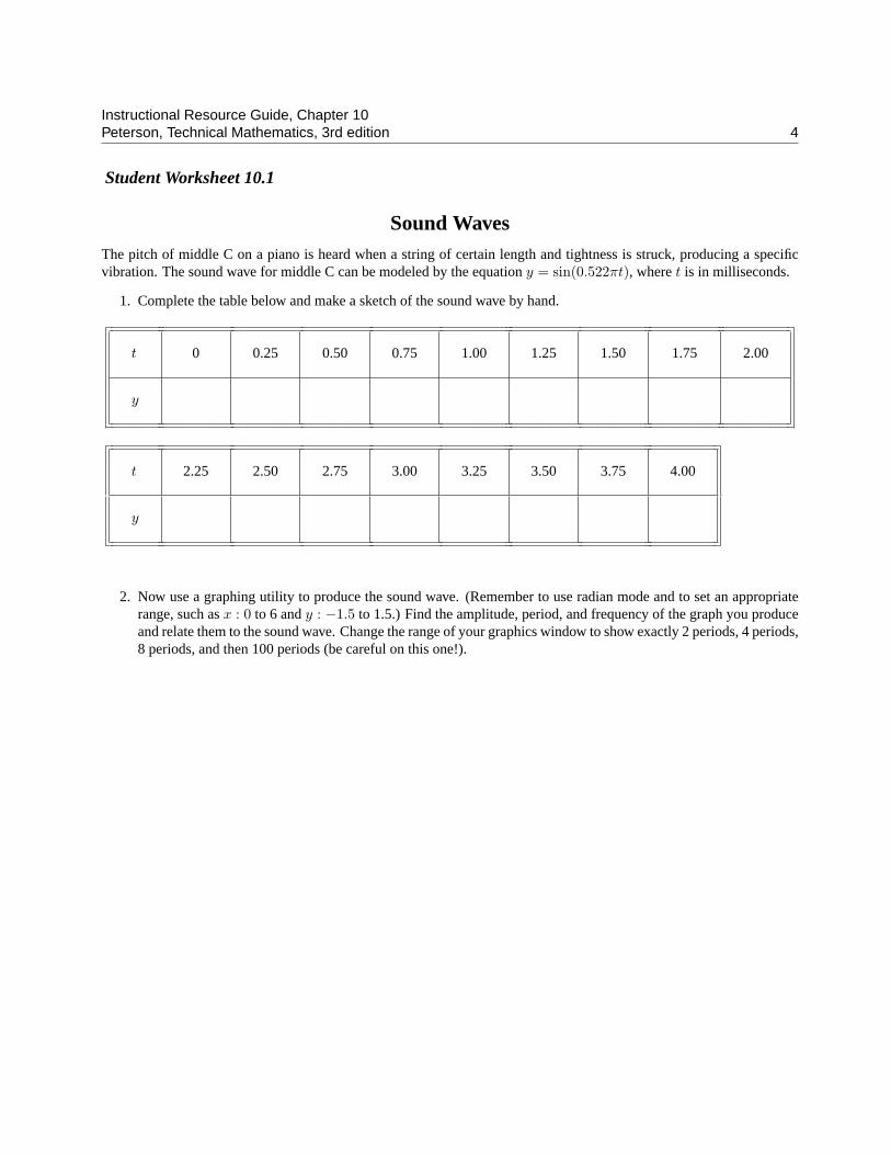
Sound WavesThe pitch of middle C on a piano is heard when a string of certain length and tightness is struck, producing a specificvibration. The sound wave for middle C can be modeled by the equationy = sin(0.522πt), wheret is in milliseconds.

1. Complete the table below and make a sketch of the sound wave by hand.

t 0 0.25 0.50 0.75 1.00 1.25 1.50 1.75 2.00

y

t 2.25 2.50 2.75 3.00 3.25 3.50 3.75 4.00

y

2. Now use a graphing utility to produce the sound wave. (Remember to use radian mode and to set an appropriaterange, such asx : 0 to 6 andy : −1.5 to 1.5.) Find the amplitude, period, and frequency of the graph you produceand relate them to the sound wave. Change the range of your graphics window to show exactly 2 periods, 4 periods,8 periods, and then 100 periods (be careful on this one!).



Discovering the Effects ofA, B, C, and D on the Graph ofy = A sin(Bt + C) + D

Rather than being given the formulas for period, amplitude, frequency, phase shifts, and vertical shifts for the func-tionsy = A sin(Bx+C)+D andy = A cos(Bx+C)+D, work in groups to complete the charts below, then recognizepatterns in the table and generalize to obtain the formulas.

Graph each function with a graphing utility and use the graph to complete the chart. After completing the chart,determine the formulas for the period, frequency, shifts, and amplitude in terms ofA, B, C, andD.

1. They = A sin(x) + D form:

A Amplitude D Vertical Shift

y = 4 sin(x)

y = 0.5 sin(x)

y = −3 sin(x)

y = sin(x) + 2

y = 3 sin(x) + 5

y = −2 sin(x) + 1

2. They = sin(Bx) form:B Period Frequency

y = sin(2x)

y = sin(4x)

y = sin(8x)

y = sin(0.5x)

y = sin(0.25x)

3. They = sin(Bx + C) form:B C Horizontal Shift

y = sin(x + π

4

)y = sin

(x − π

2

)y = sin

(2x − π

2

)y = sin

(4x − π

2

)y = sin

(x + π

2

)y = sin

(0.5x + π

2

)



Modeling Sinusoidal GraphsWrite a sine and cosine function that would model each graph shown below. For each graph, use the followingwindow settings: Xmin = 0

Xmax = 2πXscl = π/2Ymin = −5Ymax = 5Yscl = 5

.

1.

2.

3.

4.

5.

6.



Variable AmplitudeWhen two notes of similar frequency are played simultaneously, the symbolic model for the combined sound can bewritten in the form ofy = A cos(B1t) sin(B2t). SinceA cos(B1t) is the coefficient ofsin(B2t), it is the amplitude ofsin(B2t); however, since it changes value based ont values, it is called the variable amplitude. Use a graphing utility tograph the following example functions and the variable amplitude on the same screen.

Example 10.4.1 y1 = 2 cos(2x) sin(8x)y2 = 2 cos(2x)y3 = −y2 [

0, 2π, π2

]× [−2, 2, 1]

Example 10.4.2 y1 = 3 cos(3x) sin(15x)y2 = 3 cos(3x)y3 = −y2 [

0, 2π, π2

]× [−3, 3, 1]

Use a graphing utility to graph the following example functions and the variable amplitude on the same screen.

1. y1 = 2 cos(12x) sin(2x)y2 = 2 sin(2x)y3 = −y2

2. y1 = 3 cos(24x) sin(2x)y2 = 3 sin(2x)y3 = −y2

3. Do you see any patterns in the four graphical screens? Choose a hypothesis and test it with several other graphingsets of your own.



Modeling Circular Motion

Example 10.5.1 A Ferris wheel with a diameter of 50 feet makes one revolution every 12 seconds.

(a) Complete the chart below specifying distances a chair is vertically above the ground, assuming the Ferris wheelstarted when your chair was at the bottom (ground level).

(b) Plot the points on a graph.

(c) Model the graph with a sine and cosine function.

t 0 1.5 3.0 4.5 6.0 7.5 9.0 10.5 12.0

H 0

Solution

(a) Here is the completed table:

t 0 1.5 3.0 4.5 6.0 7.5 9.0 10.5 12.0

H 0 7.32 25.00 42.68 50.00 42.68 25.00 7.32 0

(b) The points from the table are plotted in Figure (a) and a curve is drawn through the points in Figure (b).

(a)[−0.1, 13, π

2

]× [−0.5, 55, 5] (b)

[−0.1, 13, π

2

]× [−0.5, 55, 5]

(c) A model that uses the cosine function isH = −25 cos(

πt6

)+ 25, where the angular velocity isπ6 rad/sec. A

model that uses the sine function isH = 25 sin(

πt6 − π

2

)+ 25, where the phase angle is−π

2 and the angularvelocity is π

6 .

After demonstrating this example, divide your class into groups and give each group a different Ferris wheel of size,angular velocity, and beginning location. Have them graph and model the heights and/or the horizontal displacementsfrom the center of the Ferris wheel. Have each group write their model on the board in a chart similar to the one below.Then, use the chart to make generalizations about circular motion with constant angular velocity.


Diameter Rotation StartingGroup (ft) (sec/rev) Location Sine Model Cosine Model

1

2

3

4

5

6



Parametric Equations and Projectile MotionSuppose that an object is thrown upward and to the right, and the data below are observed. The scatter plot of each dataset is also shown below, so we can make a guess as to what type of function could model each data set. (Technologyexists that could allow a class actually to conduct the experiment and collect such data.)

t (sec) 0 0.25 0.50 0.75 1.00

x (ft) 0 5 10 15 20

0.5 1 1.5

5

10

15

20

x

ttime

Horizontalposition

t (sec) 0 0.25 0.50 0.75 1.00

y (ft) 4 7 8 7 4

0.5 1 1.5

5

10

y

ttime

Height

Assuming the data set(t, x) is linear, the equationx = 20t can be used to model the horizontal position of the object.Assuming the data set(t, y) is quadratic, the equationy = −16(t− 0.5)22 + 8 can be used to model the vertical heightof the object. These two equations allow us to predict the location of the object at any time during the first second.

Parametric graphing allows the information given in the two graphsabove to be combined into one graph. Letting thex-axis representthe horizontal position they-axis represent the vertical height andlabeling corresponding time values on the graph puts all the graphicalinformation on one graph. This graph is shown to the right.

Now, graph the parametric set of equations on a graphing utilityand/or a spreadsheet. Trace the graph to confirm the data points pre-viously given. You may wish to change the number of points plottedby yourt-step and specify whicht-values are traced.

5 10 15 20 25

5

10

y

Horizontalposition

Height

x

t = 0

t = 0.5

t = 1.0

Exercises1. (a) Plot each of the equationsx = 104t andy = −16t2 + 104t + 50 on a regular retangualar set of axes. These

equations result when a projectile is given an initial velocity of 100 mph (147 ft per sec) at an angle of45◦ abovehorizontal and then free-falls. Remember to adjust the window settings with each new set of equations. You maywant to calculate a few(x, y) points to help decide on appropriate window settings to begin with.

(b) Graph the parametric equationsx = 104t andy = −16t2 + 104t + 50 on one graph.

2. Two motorcycles travel toward each other from Chicago and from Indianapolis, which are 350 km apart, at speeds of110 and 90 km/hr. If they start at the same time, in how many hours will they meet? Derive parametric equations for


each motorcycle and use a parametric plotting utility to graph simultaneously the location of the two motorcycles andtrace to find the time when they meet.



Spreadsheets, Polar Graphing, and Making GeneralizationsDevelop a spreadsheet that will calculate(radius, θ) values from an equation, convert the polar coordinates to rectangularcoordinates, and then plot the rectangular values. Use the spreadsheet to determine the effectB has in the polar equation(a) r = sin(Bθ), (b) r = 2 + B sin(θ), and(c) r = B + 3 sin(θ).

(Note: Depending on the experience of the student with spreadsheets, the instructor may develop the template belowfor the students. This will enable students to make only two cell changes for each new polar equation. Also, the connectedscatter plot of columns C and D should be used for the graph. Once the template is made, only change cell B2 to thefunction you wish to graph and copy cell B2 to cells B3 through B36. All the other cells should be updated automatically,including the graph. The template is shown below and three example spreadsheets follow demonstrating the effect of“B” on the graph ofr = 2 sin(Bθ).)

A B C D

θ radius x = r cos(θ) y = r sin(θ)

0 = 2 ∗ sin(2*A2) = B2*cos(A2) = B2*sin(A2)

= A2 + 0.02 = 2 ∗ sin(2*A3) = B3*cos(A3) = B3*sin(A3)



......

......




Project: Ferris Wheels and Harmonic MotionClark and Lois were excited about the fair coming to their town. Riding the Ferris wheels was their greatest thrill.Because of this, Clark was going to propose and give Lois an engagement ring while they were riding the Ferris wheel.At the fair, the crowds were so great that Clark and Lois were put on different Ferris wheels. Clark was put on the largerone and Lois was put on the smaller one. They were both at the rightmost position on each Ferris wheel when the ridebegan (t = 0). When will Clark be closest to Lois during the ride, so he can toss her the engagement ring? (Ignore theparallel distance between the two Ferris wheels.) The Ferris wheels are 11 feet apart, center-to-center, horizontally.)

11 ft

t = 0

t = 2

t = 0

t = 2

Diameter Angular Velocity

Large ferris wheel 24 1 revolution in 12 seconds

Small ferris wheel 16 1 revolution in 8 seconds

1. Complete the chart on the following page, which consists of distances between Clark and Lois at various times.

2. Write functions for the location of Clark’s position and the location of Lois’s position.

3. Using the above functions, write a function that represents the distance between Clark and Lois.

4. Graph the distance function from Exercise 3 and locate the time and position Clark and Lois are the closest. (Hint:Use parametric graphing with Clark’s position as the first equation, Lois’s position as the second equation and thedistance function as the third equation. Write the distance in terms ofxt1, xt2, yt1, andyt.)

Notice that this table assumes that the origin is at the bottom of the larger Ferris wheel.


Time Clark’s Position Lois’s Position Distance Between Them (ft)

0 (12, 12) (19, 8)√

(19− 12)2 + (8− 12)2 ≈ 8.06

2 (6, 22.39) (11, 16)

4

6

8

10

12

14

16


Note: This project also applies to Chapter 20: Trigonometric Formulas, Identities, and Equations. It could beassigned as a project that applies trigonometric identities.

Project: Sound Applications of Trig Functions

Solutions

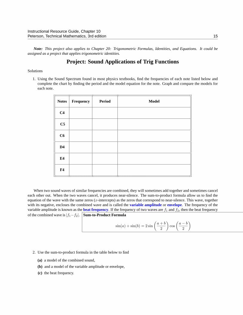
1. Using the Sound Spectrum found in most physics textbooks, find the frequencies of each note listed below andcomplete the chart by finding the period and the model equation for the note. Graph and compare the models foreach note.

Notes Frequency Period Model

C4

C5

C6

D4

E4

F4

When two sound waves of similar frequencies are combined, they will sometimes add together and sometimes canceleach other out. When the two waves cancel, it produces near-silence. The sum-to-product formula allow us to find theequation of the wave with the same zeros (x-intercepts) as the zeros that correspond to near-silence. This wave, togetherwith its negative, encloses the combined wave and is called thevariable amplitude or envelope. The frequency of thevariable amplitude is known as thebeat frequency. If the frequency of two waves aref1 andf2, then the beat frequencyof the combined wave is|f1−f2|. Sum-to-Product Formula

sin(a) + sin(b) = 2 sin(

a + b

2

)cos

(a− b

2

)

2. Use the sum-to-product formula in the table below to find

(a) a model of the combined sound,

(b) and a model of the variable amplitude or envelope,

(c) the beat frequency.


Notes Combined Model Envelope Model Beat Frequency

C4 & C5

C5 & C6

C4 & C6

C4 & D4

C4 & E4

C4 & F4

3. Graph the combined model with the envelope model to confirm the relationship between the models and the beatfrequency.

Answers


1.t 0 0.25 0.50 0.75 1.00 1.25 1.50 1.75 2.00

y 0 0.399 0.731 0.942 0.998 0.887 0.630 0.268 −0.138

t 2.25 2.50 2.75 3.00 3.25 3.50 3.75 4.00

y −0.521 −0.818 −0.980 −0.979 −0.815 −0.517 −0.133 0.273

2.

[0, 6]× [−1.5, 1.5]The amplitude is1, the period is 2π

0.522 = π0.261 ≈ 12.037, and the frequency is0.522

2π = 0.261π ≈ 0.831.

[0, 7.663]× [−1.5, 1.5]2 periods

[0, 15.326]× [−1.5, 1.5]4 periods

17

Instructional Resource Guide, AnswersPeterson, Technical Mathematics, 3rd edition 18

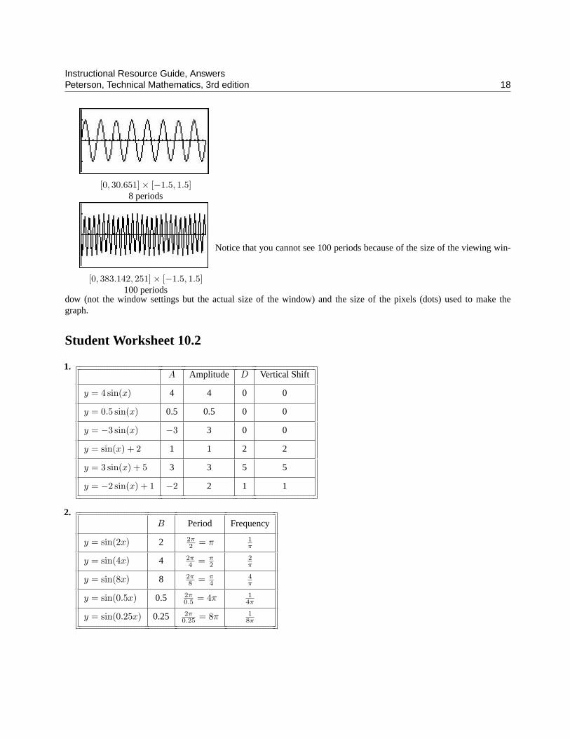
[0, 30.651]× [−1.5, 1.5]8 periods

[0, 383.142, 251]× [−1.5, 1.5]100 periods

Notice that you cannot see 100 periods because of the size of the viewing win-

dow (not the window settings but the actual size of the window) and the size of the pixels (dots) used to make thegraph.


1.A Amplitude D Vertical Shift

y = 4 sin(x) 4 4 0 0

y = 0.5 sin(x) 0.5 0.5 0 0

y = −3 sin(x) −3 3 0 0

y = sin(x) + 2 1 1 2 2

y = 3 sin(x) + 5 3 3 5 5

y = −2 sin(x) + 1 −2 2 1 1

2.B Period Frequency

y = sin(2x) 2 2π2 = π 1

π

y = sin(4x) 4 2π4 = π

22π

y = sin(8x) 8 2π8 = π

44π

y = sin(0.5x) 0.5 2π0.5 = 4π 1

4π

y = sin(0.25x) 0.25 2π0.25 = 8π 1

8π


3.B C Horizontal Shift

y = sin(x + π

4

)1 π

4 −π4

y = sin(x− π

2

)1 −π

2π2

y = sin(2x− π

2

)2 −π

4π8

y = sin(4x− π

2

)4 −π

8π32

y = sin(x + π

2

)1 π

2 −π2

y = sin(0.5x + π

2

)0.5 π −2π


1. y = 3 sin(4x)

2. y = 4 cos(2x)

3. y = −2 cos(0.5x)

4. y = 2 cos(0.5x + π

4

)5. y = 2 sin (3x) + 2

6. y = 3 cos (6x)− 2


1. The first graph was made using a TI-86 and the second graph shows the different functions in color so you can betterdifferentiate them.

[0, 2π, π

2

]× [−2, 2, 1]

π 2 π

1

−1

y

x

y = 2 cos(2x) sin(2x) is in blue,y = 2 sin(2x) is in green, and

y = −2 sin(2x) is in red.

2. The first graph was made using a TI-86 and the second graph shows the different functions in color so you can betterdifferentiate them.


[0, 2π, π

2

]× [−3, 3, 1]

π 2 π

1

2

3

−1

−2

−3

y

x

y = 3 cos(3x) sin(15x)is in blue,y = 3 sin(3x) is in green, and

y = −3 sin(3x) is in red.

3. All four graphs have periodB1π whereB1 < B2 andB2 is a multiple ofB1.


1. (a)

[0, 7, 1]× [0, 750, 50]x = 104t

[0, 7, 1]× [0, 225, 25]y = −16t2 + 104t + 50

(b)

[0, 750, 50]× [0, 225, 25]x = 104t andy = −16t2 + 104t + 50

2. For motorcycle #1, the one that travels at 110 km/hr, theequations arex = t, y = 110t and for the second motor-cycle the equations arex = t, y = 350 − 90t, wheret isin hours andy in km. As you can see from the figure be-low, they intersect whent = 1.75 hr. At that time the firstmotorcycle is 192.5 km from its starting city. The secondmotorcycle is350− 192.5 = 157.5 from its starting city.

[0, 4, 1]× [0, 350, 25]x = 104t andy = −16t2 + 104t + 50



1.Time Clark’s Position Lois’s Position Distance Between Them (ft)

0 (12, 12) (19, 8)√

(19− 12)2 + (8− 12)2 ≈ 8.06

2 (6, 22.39) (11, 16)√

(11− 6)2 + (16− 22.39)2 ≈ 8.12

4 (−6, 22.39) (3, 8) ≈ 16.97

6 (−12, 12) (11, 0) ≈ 25.94

8 (−6, 1.61) (19, 8) ≈ 25.80

10 (6, 1.61) (11, 16) ≈ 15.24

12 (12, 12) (3, 8) ≈ 9.85

14 (6, 22.39) (11, 0) ≈ 22.94

16 (−6, 22.39) (19, 8) ≈ 26.85

2. Parametric equations for Clark’s position are:

{xC(t) = 12 cos

(πt6

)yC(t) = 12 sin

(πt6

)+ 12

and for Lois the parametric equations

are:

{xL(t) = 8 cos

(πt4

)+ 11

yL(t) = 8 sin(

πt4

)+ 8

.

3. The distance between Clark and Lois isd =√

(xC(t)− xL(t))2 + (yC(t)− yL(t))2

4. From this graph, we see that whent ≈ 21.57 sec they are only 4.82 ft apart.

1. In this table, the frequencies have been rounded to the nearest whole number.

Notes Frequency Period Model in radians

C4 262 1262 sin(524πt)

C5 523 1523 sin(1026πt)

C6 1026 11026 sin(2052πt)

D4 311 1311 sin(622πt)

E4 330 1330 sin(660πt)

F4 349 1349 sin(698πt)


2.

Notes Combined Model Envelope Model Beat Frequency (Hz)

C4 & C5 2 sin(775πt) cos(251πt) 2 cos(251πt) 251



C4 & D4 2 sin(573πt) cos(49πt) 2 cos(49πt) 49

C4 & E4 2 sin(592πt) cos(68πt) 2 cos(68πt) 49

C4 & F4 2 sin(611πt) cos(87πt) 2 cos(87πt) 87

3.

Notes C4 and C5

Notes C5 and C6

Notes C4 and C6

Notes C4 and D4

Notes C4 and E4


Notes C4 and F4


1. In this table, the frequencies have been rounded to the nearest whole number.

Notes Frequency Period Model

C4 262 1262 sin(524πt) in radians

C5 523

C6 1026

D4 311

E4 330

F4 349

Documents

Contents - Brands Delmar - Cengage · PDF fileContents How You May Use This ... Ferris Wheels and Harmonic Motion . . . . . . . . . 13 Worksheet 10.8: ... • Classify applications