Embed Size (px)
Citation preview
Contents
4 Statistical Ensembles 1
4.1 References . . . . . . . . . . . . . . . . . . . . . . . . . . . . . . . . . . . . . . . . . . . . . . . . . . . . 1
4.2 Microcanonical Ensemble (µCE) . . . . . . . . . . . . . . . . . . . . . . . . . . . . . . . . . . . . . . . 2
4.2.1 The microcanonical distribution function . . . . . . . . . . . . . . . . . . . . . . . . . . . . . . 2
4.2.2 Density of states . . . . . . . . . . . . . . . . . . . . . . . . . . . . . . . . . . . . . . . . . . . . 3
4.2.3 Arbitrariness in the definition of S(E) . . . . . . . . . . . . . . . . . . . . . . . . . . . . . . . 5
4.2.4 Ultra-relativistic ideal gas . . . . . . . . . . . . . . . . . . . . . . . . . . . . . . . . . . . . . . 6
4.2.5 Discrete systems . . . . . . . . . . . . . . . . . . . . . . . . . . . . . . . . . . . . . . . . . . . . 6
4.3 The Quantum Mechanical Trace . . . . . . . . . . . . . . . . . . . . . . . . . . . . . . . . . . . . . . . 6
4.3.1 The density matrix . . . . . . . . . . . . . . . . . . . . . . . . . . . . . . . . . . . . . . . . . . 7
4.3.2 Averaging the DOS . . . . . . . . . . . . . . . . . . . . . . . . . . . . . . . . . . . . . . . . . . 8
4.3.3 Coherent states . . . . . . . . . . . . . . . . . . . . . . . . . . . . . . . . . . . . . . . . . . . . . 8
4.4 Thermal Equilibrium . . . . . . . . . . . . . . . . . . . . . . . . . . . . . . . . . . . . . . . . . . . . . . 10
4.5 Ordinary Canonical Ensemble (OCE) . . . . . . . . . . . . . . . . . . . . . . . . . . . . . . . . . . . . 12
4.5.1 Canonical distribution and partition function . . . . . . . . . . . . . . . . . . . . . . . . . . . 12
4.5.2 The difference between P (En) and Pn . . . . . . . . . . . . . . . . . . . . . . . . . . . . . . . 13
4.5.3 Averages within the OCE . . . . . . . . . . . . . . . . . . . . . . . . . . . . . . . . . . . . . . . 13
4.5.4 Entropy and free energy . . . . . . . . . . . . . . . . . . . . . . . . . . . . . . . . . . . . . . . 14
4.5.5 Fluctuations in the OCE . . . . . . . . . . . . . . . . . . . . . . . . . . . . . . . . . . . . . . . 15
4.5.6 Thermodynamics revisited . . . . . . . . . . . . . . . . . . . . . . . . . . . . . . . . . . . . . . 16
4.5.7 Generalized susceptibilities . . . . . . . . . . . . . . . . . . . . . . . . . . . . . . . . . . . . . 17
4.6 Grand Canonical Ensemble (GCE) . . . . . . . . . . . . . . . . . . . . . . . . . . . . . . . . . . . . . . 18
4.6.1 Grand canonical distribution and partition function . . . . . . . . . . . . . . . . . . . . . . . 18
i
ii CONTENTS
4.6.2 Entropy and Gibbs-Duhem relation . . . . . . . . . . . . . . . . . . . . . . . . . . . . . . . . . 19
4.6.3 Generalized susceptibilities in the GCE . . . . . . . . . . . . . . . . . . . . . . . . . . . . . . . 20
4.6.4 Fluctuations in the GCE . . . . . . . . . . . . . . . . . . . . . . . . . . . . . . . . . . . . . . . . 21
4.6.5 Gibbs ensemble . . . . . . . . . . . . . . . . . . . . . . . . . . . . . . . . . . . . . . . . . . . . 21
4.7 Statistical Ensembles from Maximum Entropy . . . . . . . . . . . . . . . . . . . . . . . . . . . . . . . 22
4.7.1 µCE . . . . . . . . . . . . . . . . . . . . . . . . . . . . . . . . . . . . . . . . . . . . . . . . . . . 22
4.7.2 OCE . . . . . . . . . . . . . . . . . . . . . . . . . . . . . . . . . . . . . . . . . . . . . . . . . . . 23
4.7.3 GCE . . . . . . . . . . . . . . . . . . . . . . . . . . . . . . . . . . . . . . . . . . . . . . . . . . . 23
4.8 Ideal Gas Statistical Mechanics . . . . . . . . . . . . . . . . . . . . . . . . . . . . . . . . . . . . . . . . 24
4.8.1 Maxwell velocity distribution . . . . . . . . . . . . . . . . . . . . . . . . . . . . . . . . . . . . 25
4.8.2 Equipartition . . . . . . . . . . . . . . . . . . . . . . . . . . . . . . . . . . . . . . . . . . . . . . 26
4.8.3 Quantum statistics and the Maxwell-Boltzmann limit . . . . . . . . . . . . . . . . . . . . . . 27
4.9 Selected Examples . . . . . . . . . . . . . . . . . . . . . . . . . . . . . . . . . . . . . . . . . . . . . . . 28
4.9.1 Spins in an external magnetic field . . . . . . . . . . . . . . . . . . . . . . . . . . . . . . . . . 28
4.9.2 Negative temperature (!) . . . . . . . . . . . . . . . . . . . . . . . . . . . . . . . . . . . . . . . 30
4.9.3 Adsorption . . . . . . . . . . . . . . . . . . . . . . . . . . . . . . . . . . . . . . . . . . . . . . . 31
4.9.4 Elasticity of wool . . . . . . . . . . . . . . . . . . . . . . . . . . . . . . . . . . . . . . . . . . . 32
4.9.5 Noninteracting spin dimers . . . . . . . . . . . . . . . . . . . . . . . . . . . . . . . . . . . . . 34
4.10 Statistical Mechanics of Molecular Gases . . . . . . . . . . . . . . . . . . . . . . . . . . . . . . . . . . 35
4.10.1 Separation of translational and internal degrees of freedom . . . . . . . . . . . . . . . . . . . 35
4.10.2 Ideal gas law . . . . . . . . . . . . . . . . . . . . . . . . . . . . . . . . . . . . . . . . . . . . . . 37
4.10.3 The internal coordinate partition function . . . . . . . . . . . . . . . . . . . . . . . . . . . . . 37
4.10.4 Rotations . . . . . . . . . . . . . . . . . . . . . . . . . . . . . . . . . . . . . . . . . . . . . . . . 37
4.10.5 Vibrations . . . . . . . . . . . . . . . . . . . . . . . . . . . . . . . . . . . . . . . . . . . . . . . . 39
4.10.6 Two-level systems : Schottky anomaly . . . . . . . . . . . . . . . . . . . . . . . . . . . . . . . 40
4.10.7 Electronic and nuclear excitations . . . . . . . . . . . . . . . . . . . . . . . . . . . . . . . . . . 42
4.11 Appendix I : Additional Examples . . . . . . . . . . . . . . . . . . . . . . . . . . . . . . . . . . . . . . 44
4.11.1 Three state system . . . . . . . . . . . . . . . . . . . . . . . . . . . . . . . . . . . . . . . . . . . 44
4.11.2 Spins and vacancies on a surface . . . . . . . . . . . . . . . . . . . . . . . . . . . . . . . . . . 44
4.11.3 Fluctuating interface . . . . . . . . . . . . . . . . . . . . . . . . . . . . . . . . . . . . . . . . . 46
4.11.4 Dissociation of molecular hydrogen . . . . . . . . . . . . . . . . . . . . . . . . . . . . . . . . . 48
Chapter 4
Statistical Ensembles
4.1 References
– F. Reif, Fundamentals of Statistical and Thermal Physics (McGraw-Hill, 1987)This has been perhaps the most popular undergraduate text since it first appeared in 1967, and with goodreason.
– A. H. Carter, Classical and Statistical Thermodynamics(Benjamin Cummings, 2000)A very relaxed treatment appropriate for undergraduate physics majors.
– D. V. Schroeder, An Introduction to Thermal Physics (Addison-Wesley, 2000)This is the best undergraduate thermodynamics book I’ve come across, but only 40% of the book treatsstatistical mechanics.
– C. Kittel, Elementary Statistical Physics (Dover, 2004)Remarkably crisp, though dated, this text is organized as a series of brief discussions of key concepts andexamples. Published by Dover, so you can’t beat the price.
– M. Kardar, Statistical Physics of Particles (Cambridge, 2007)A superb modern text, with many insightful presentations of key concepts.
– M. Plischke and B. Bergersen, Equilibrium Statistical Physics (3rd edition, World Scientific, 2006)An excellent graduate level text. Less insightful than Kardar but still a good modern treatment of the subject.Good discussion of mean field theory.
– E. M. Lifshitz and L. P. Pitaevskii, Statistical Physics (part I, 3rd edition, Pergamon, 1980)This is volume 5 in the famous Landau and Lifshitz Course of Theoretical Physics. Though dated, it stillcontains a wealth of information and physical insight.
1
2 CHAPTER 4. STATISTICAL ENSEMBLES
4.2 Microcanonical Ensemble (µCE)
4.2.1 The microcanonical distribution function
We have seen how in an ergodic dynamical system, time averages can be replaced by phase space averages:
ergodicity ⇐⇒⟨f(ϕ)
⟩T
=⟨f(ϕ)
⟩S, (4.1)
where
⟨f(ϕ)
⟩T
= limT→∞
1
T
T∫
0
dt f(ϕ(t)
). (4.2)
and⟨f(ϕ)
⟩S
=
∫dµ f(ϕ) δ
(E − H(ϕ)
)/∫dµ δ
(E − H(ϕ)
). (4.3)
Here H(ϕ) = H(q,p) is the Hamiltonian, and where δ(x) is the Dirac δ-function1. Thus, averages are taken overa constant energy hypersurface which is a subset of the entire phase space.
We’ve also seen how any phase space distribution (Λ1, . . . , Λk) which is a function of conserved quantitied Λa(ϕ)is automatically a stationary (time-independent) solution to Liouville’s equation. Note that the microcanonicaldistribution,
E(ϕ) = δ(E − H(ϕ)
)/∫dµ δ
(E − H(ϕ)
), (4.4)
is of this form, since H(ϕ) is conserved by the dynamics. Linear and angular momentum conservation generallyare broken by elastic scattering off the walls of the sample.
So averages in the microcanonical ensemble are computed by evaluating the ratio
⟨A⟩
=Tr Aδ(E − H)
Tr δ(E − H), (4.5)
where Tr means ‘trace’, which entails an integration over all phase space:
Tr A(q, p) ≡ 1
N !
N∏
i=1
∫ddpi d
dqi(2π~)d
A(q, p) . (4.6)
Here N is the total number of particles and d is the dimension of physical space in which each particle moves.The factor of 1/N !, which cancels in the ratio between numerator and denominator, is present for indistinguishableparticles. The normalization factor (2π~)−Nd renders the trace dimensionless. Again, this cancels between numer-ator and denominator. These factors may then seem arbitrary in the definition of the trace, but we’ll see how theyin fact are required from quantum mechanical considerations. So we now adopt the following metric for classicalphase space integration:
dµ =1
N !
N∏
i=1
ddpi ddqi
(2π~)d. (4.7)
1We write the Hamiltonian as H (classical or quantum) in order to distinguish it from magnetic field (H) or enthalpy (H).
4.2. MICROCANONICAL ENSEMBLE (µCE) 3
4.2.2 Density of states
The denominator,D(E) = Tr δ(E − H) , (4.8)
is called the density of states. It has dimensions of inverse energy, such that
D(E)∆E =
E+∆E∫
E
dE′
∫dµ δ(E′ − H) =
∫
E<H<E+∆E
dµ (4.9)
= # of states with energies between E and E + ∆E .
Let us now compute D(E) for the nonrelativistic ideal gas. The Hamiltonian is
H(q, p) =
N∑
i=1
p2i
2m. (4.10)
We assume that the gas is enclosed in a region of volume V , and we’ll do a purely classical calculation, neglectingdiscreteness of its quantum spectrum. We must compute
D(E) =1
N !
∫ N∏
i=1
ddpi ddqi
(2π~)dδ
(E −
N∑
i=1
p2i
2m
). (4.11)
We’ll do this calculation in two ways. First, let’s rescale pαi ≡
√2mE uα
i . We then have
D(E) =V N
N !
(√2mE
h
)Nd1
E
∫dMu δ
(u2
1 + u22 + . . .+ u2
M − 1). (4.12)
Here we have written u = (u1, u2, . . . , uM ) with M = Nd as a M -dimensional vector. We’ve also used the ruleδ(Ex) = E−1δ(x) for δ-functions. We can now write
dMu = uM−1 du dΩM , (4.13)
where dΩM is the M -dimensional differential solid angle. We now have our answer:2
D(E) =V N
N !
(√2m
h
)Nd
E12Nd−1 · 1
2 ΩNd . (4.14)
What remains is for us to compute ΩM , the total solid angle in M dimensions. We do this by a nifty mathematicaltrick. Consider the integral
IM =
∫dMu e−u2
= ΩM
∞∫
0
du uM−1 e−u2
= 12ΩM
∞∫
0
ds s12M−1
e−s = 12ΩM Γ
(12M
),
(4.15)
2The factor of 12
preceding ΩM
in eqn. 4.14 appears because δ(u2 − 1) = 12
δ(u − 1) + 12
δ(u + 1). Since u = |u| ≥ 0, the second term canbe dropped.
4 CHAPTER 4. STATISTICAL ENSEMBLES
where s = u2, and where
Γ(z) =
∞∫
0
dt tz−1 e−t (4.16)
is the Gamma function, which satisfies z Γ(z) = Γ(z + 1).3 On the other hand, we can compute IM in Cartesiancoordinates, writing
IM =
∞∫
−∞
du1 e−u2
1
M
=(√π)M
. (4.17)
Therefore
ΩM =2πM/2
Γ(M/2). (4.18)
We thereby obtain Ω2 = 2π, Ω3 = 4π, Ω4 = 2π2, etc., the first two of which are familiar.
Our final result, then, is
D(E, V,N) =V N
N !
(m
2π~2
)Nd/2 E12Nd−1
Γ(Nd/2). (4.19)
Here we have emphasized that the density of states is a function of E, V , and N . Using Stirling’s approximation,
lnN ! = N lnN −N + 12 lnN + 1
2 ln(2π) + O(N−1
), (4.20)
we may define the statistical entropy,
S(E, V,N) ≡ kB
lnD(E, V,N) = NkBφ
(E
N,V
N
)+ O(lnN) , (4.21)
where
φ
(E
N,V
N
)=d
2ln
(E
N
)+ ln
(V
N
)+d
2ln
(m
dπ~2
)+(1 + 1
2d). (4.22)
Recall kB
= 1.3806503× 10⁻¹⁶ erg/K is Boltzmann’s constant.
The second way to calculate D(E) is to first compute its Laplace transform, Z(β):
Z(β) = L[D(E)
]≡
∞∫
0
dE e−βE D(E) = Tr e−βH . (4.23)
The inverse Laplace transform is then
D(E) = L−1[Z(β)
]≡
c+i∞∫
c−i∞
dβ
2πieβE Z(β) , (4.24)
where c is such that the integration contour is to the right of any singularities of Z(β) in the complex β-plane. We
3Note that for integer argument, Γ(k) = (k − 1)!
4.2. MICROCANONICAL ENSEMBLE (µCE) 5
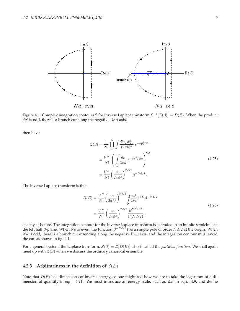
Figure 4.1: Complex integration contours C for inverse Laplace transform L−1[Z(β)
]= D(E). When the product
dN is odd, there is a branch cut along the negative Re β axis.
then have
Z(β) =1
N !
N∏
i=1
∫ddxi d
dpi
(2π~)de−βp2
i /2m
=V N
N !
∞∫
−∞
dp
2π~e−βp2/2m
Nd
=V N
N !
(m
2π~2
)Nd/2
β−Nd/2 .
(4.25)
The inverse Laplace transform is then
D(E) =V N
N !
(m
2π~2
)Nd/2 ∮
C
dβ
2πieβE β−Nd/2
=V N
N !
(m
2π~2
)Nd/2 E12Nd−1
Γ(Nd/2),
(4.26)
exactly as before. The integration contour for the inverse Laplace transform is extended in an infinite semicircle inthe left half β-plane. When Nd is even, the function β−Nd/2 has a simple pole of order Nd/2 at the origin. WhenNd is odd, there is a branch cut extending along the negative Reβ axis, and the integration contour must avoidthe cut, as shown in fig. 4.1.
For a general system, the Laplace transform, Z(β) = L[D(E)
]also is called the partition function. We shall again
meet up with Z(β) when we discuss the ordinary canonical ensemble.
4.2.3 Arbitrariness in the definition of S(E)
Note that D(E) has dimensions of inverse energy, so one might ask how we are to take the logarithm of a di-mensionful quantity in eqn. 4.21. We must introduce an energy scale, such as ∆E in eqn. 4.9, and define
6 CHAPTER 4. STATISTICAL ENSEMBLES
D(E; ∆E) = D(E)∆E and S(E; ∆E) ≡ kB
ln D(E; ∆E). The definition of statistical entropy then involves thearbitrary parameter ∆E, however this only affects S(E) in an additive way. That is,
S(E, V,N ; ∆E1) = S(E, V,N ; ∆E2) + kB
ln
(∆E1
∆E2
). (4.27)
Note that the difference between the two definitions of S depends only on the ratio ∆E1/∆E2, and is independentof E, V , and N .
4.2.4 Ultra-relativistic ideal gas
Consider an ultrarelativistic ideal gas, with single particle dispersion ε(p) = cp. We then have
Z(β) =V N
N !
ΩNd
hNd
∞∫
0
dp pd−1 e−βcp
N
=V N
N !
(Γ(d)Ωd
cd hd βd
)N.
(4.28)
The statistical entropy is S(E, V,N) = kB
lnD(E, V,N) = NkBφ(
EN ,
VN
), with
φ
(E
N,V
N
)= d ln
(E
N
)+ ln
(V
N
)+ ln
(Ωd Γ(d)
(dhc)d
)+ (d+ 1) (4.29)
4.2.5 Discrete systems
For classical systems where the energy levels are discrete, the states of the system |σ 〉 are labeled by a set ofdiscrete quantities σ1, σ2, . . ., where each variable σi takes discrete values. The number of ways of configuringthe system at fixed energy E is then
Ω(E,N) =∑
σ
δH(σ),E
, (4.30)
where the sum is over all possible configurations. Here N labels the total number of particles. For example, ifwe have N spin- 1
2 particles on a lattice which are placed in a magnetic field H , so the individual particle energyis εi = −µ0Hσ, where σ = ±1, then in a configuration in which N↑ particles have σi = +1 and N↓ = N − N↑
particles have σi = −1, the energy is E = (N↓ −N↑)µ0H . The number of configurations at fixed energy E is
Ω(E,N) =
(N
N↑
)=
N !(N2 − E
2µ0H
)!(
N2 + E
2µ0H
)!, (4.31)
since N↑/↓ = N2 ∓ E
2µ0H . The statistical entropy is S(E,N) = kB
ln Ω(E,N).
4.3 The Quantum Mechanical Trace
Thus far our understanding of ergodicity is rooted in the dynamics of classical mechanics. A Hamiltonian flowwhich is ergodic is one in which time averages can be replaced by phase space averages using the microcanonicalensemble. What happens, though, if our system is quantum mechanical, as all systems ultimately are?
4.3. THE QUANTUM MECHANICAL TRACE 7
4.3.1 The density matrix
First, let us consider that our system S will in general be in contact with a world W . We call the union of S andW the universe, U = W ∪ S. Let
∣∣N⟩
denote a quantum mechanical state of W , and let∣∣n⟩
denote a quantummechanical state of S. Then the most general wavefunction we can write is of the form
∣∣Ψ⟩
=∑
N,n
ΨN,n
∣∣N⟩⊗∣∣n⟩. (4.32)
Now let us compute the expectation value of some operator A which acts as the identity within W , meaning⟨N∣∣ A∣∣N ′
⟩= A δNN ′ , where A is the ‘reduced’ operator which acts within S alone. We then have
⟨Ψ∣∣ A∣∣Ψ⟩
=∑
N,N ′
∑
n,n′
Ψ∗N,n ΨN ′,n′ δNN ′
⟨n∣∣ A∣∣n′⟩
= Tr(ˆA),
(4.33)
whereˆ =
∑
N
∑
n,n′
Ψ∗N,n ΨN,n′
∣∣n′⟩ ⟨n∣∣ (4.34)
is the density matrix. The time-dependence of ˆ is easily found:
ˆ(t) =∑
N
∑
n,n′
Ψ∗N,n ΨN,n′
∣∣n′(t)⟩ ⟨n(t)
∣∣
= e−iHt/~ ˆ e+iHt/~ ,
(4.35)
where H is the Hamiltonian for the system S. Thus, we find
i~∂ ˆ
∂t=[H, ˆ
]. (4.36)
Note that the density matrix evolves according to a slightly different equation than an operator in the Heisenbergpicture, for which
A(t) = e+iHt/~ Ae−iHt/~ =⇒ i~∂A
∂t=[A, H
]= −
[H, A
]. (4.37)
For Hamiltonian systems, we found that the phase space distribution (q, p, t) evolved according to the Liouvilleequation,
i∂
∂t= L , (4.38)
where the Liouvillian L is the differential operator
L = −iNd∑
j=1
∂H
∂pj
∂
∂qj− ∂H
∂qj
∂
∂pj
. (4.39)
Accordingly, any distribution (Λ1, . . . , Λk) which is a function of constants of the motion Λa(q, p) is a station-ary solution to the Liouville equation: ∂t (Λ1, . . . , Λk) = 0. Similarly, any quantum mechanical density matrixwhich commutes with the Hamiltonian is a stationary solution to eqn. 4.36. The corresponding microcanonicaldistribution is
ˆE = δ(E − H
). (4.40)
8 CHAPTER 4. STATISTICAL ENSEMBLES
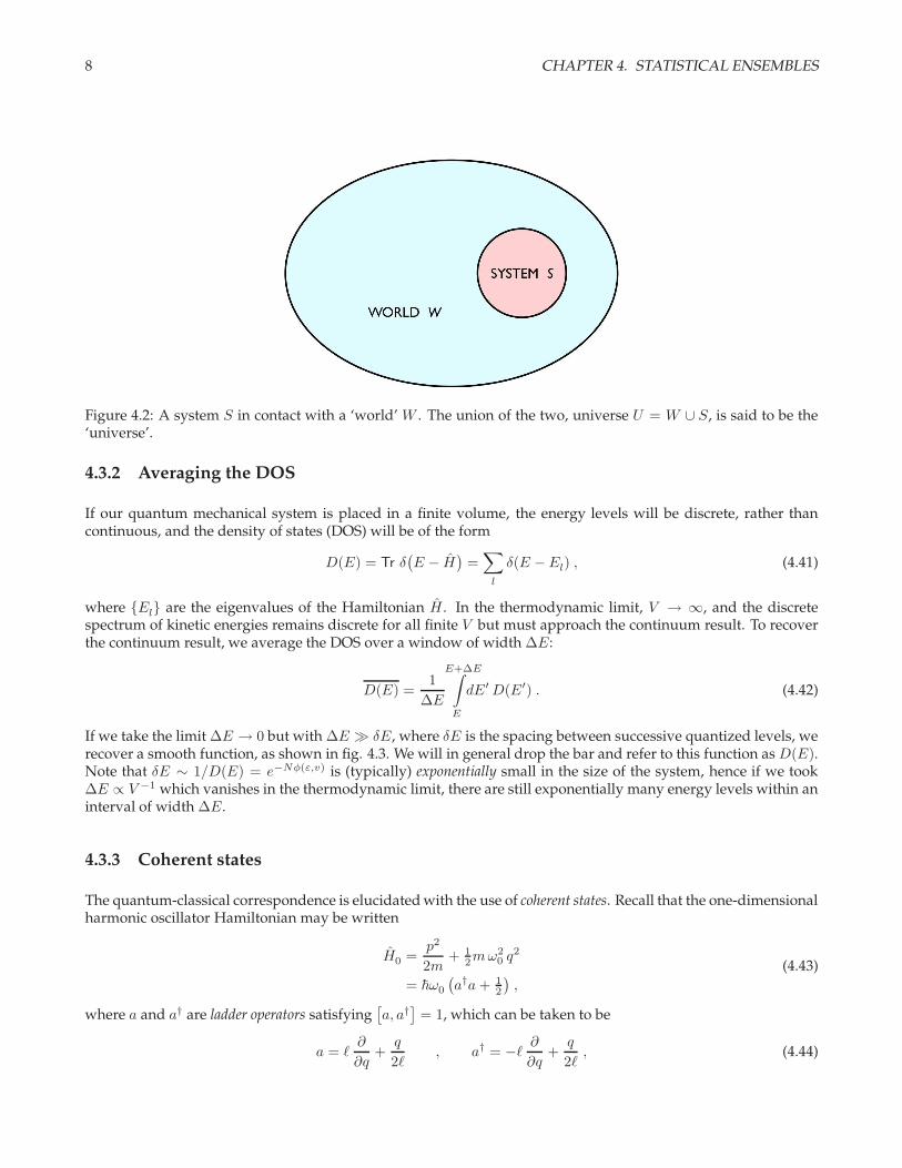
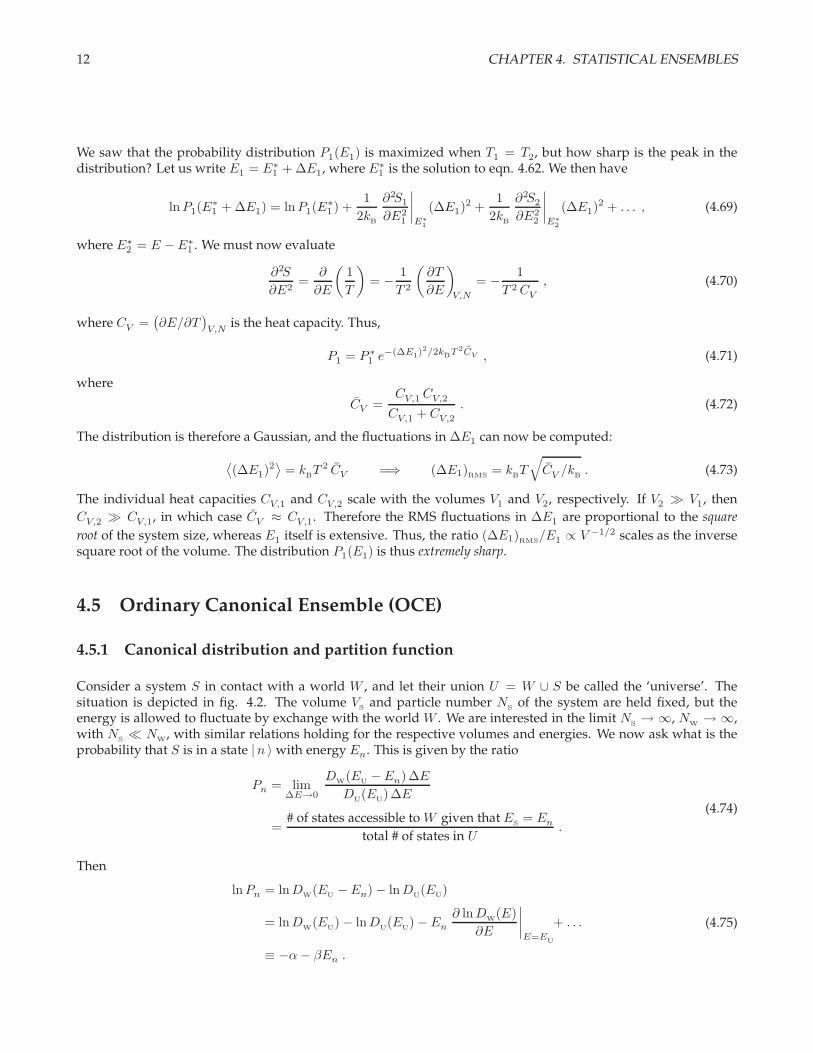
Figure 4.2: A system S in contact with a ‘world’ W . The union of the two, universe U = W ∪ S, is said to be the‘universe’.
4.3.2 Averaging the DOS
If our quantum mechanical system is placed in a finite volume, the energy levels will be discrete, rather thancontinuous, and the density of states (DOS) will be of the form
D(E) = Tr δ(E − H
)=∑
l
δ(E − El) , (4.41)
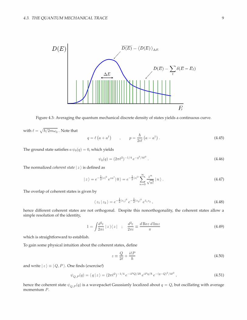
where El are the eigenvalues of the Hamiltonian H . In the thermodynamic limit, V → ∞, and the discretespectrum of kinetic energies remains discrete for all finite V but must approach the continuum result. To recoverthe continuum result, we average the DOS over a window of width ∆E:
D(E) =1
∆E
E+∆E∫
E
dE′D(E′) . (4.42)
If we take the limit ∆E → 0 but with ∆E ≫ δE, where δE is the spacing between successive quantized levels, werecover a smooth function, as shown in fig. 4.3. We will in general drop the bar and refer to this function as D(E).Note that δE ∼ 1/D(E) = e−Nφ(ε,v) is (typically) exponentially small in the size of the system, hence if we took∆E ∝ V −1 which vanishes in the thermodynamic limit, there are still exponentially many energy levels within aninterval of width ∆E.
4.3.3 Coherent states
The quantum-classical correspondence is elucidated with the use of coherent states. Recall that the one-dimensionalharmonic oscillator Hamiltonian may be written
H0 =p2
2m+ 1
2mω20 q
2
= ~ω0
(a†a+ 1
2
),
(4.43)
where a and a† are ladder operators satisfying[a, a†
]= 1, which can be taken to be
a = ℓ∂
∂q+
q
2ℓ, a† = −ℓ ∂
∂q+
q
2ℓ, (4.44)
4.3. THE QUANTUM MECHANICAL TRACE 9
Figure 4.3: Averaging the quantum mechanical discrete density of states yields a continuous curve.
with ℓ =√
~/2mω0 . Note that
q = ℓ(a+ a†
), p =
~
2iℓ
(a− a†
). (4.45)
The ground state satisfies aψ0(q) = 0, which yields
ψ0(q) = (2πℓ2)−1/4 e−q2/4ℓ2 . (4.46)
The normalized coherent state | z 〉 is defined as
| z 〉 = e−12 |z|2 eza† | 0 〉 = e−
12 |z|2
∞∑
n=0
zn
√n!
|n 〉 . (4.47)
The overlap of coherent states is given by
〈 z1 | z2 〉 = e−12 |z1|
2
e−12 |z2|
2
ez1z2 , (4.48)
hence different coherent states are not orthogonal. Despite this nonorthogonality, the coherent states allow asimple resolution of the identity,
1 =
∫d2z
2πi| z 〉〈 z | ;
d2z
2πi≡ dRez d Imz
π(4.49)
which is straightforward to establish.
To gain some physical intuition about the coherent states, define
z ≡ Q
2ℓ+iℓP
~(4.50)
and write | z 〉 ≡ |Q,P 〉. One finds (exercise!)
ψQ,P (q) = 〈 q | z 〉 = (2πℓ2)−1/4 e−iPQ/2~ eiPq/~ e−(q−Q)2/4ℓ2 , (4.51)
hence the coherent state ψQ,P (q) is a wavepacket Gaussianly localized about q = Q, but oscillating with averagemomentum P .
10 CHAPTER 4. STATISTICAL ENSEMBLES
For example, we can compute
⟨Q,P
∣∣ q∣∣Q,P
⟩=⟨z∣∣ ℓ (a+ a†)
∣∣ z⟩
= 2ℓ Re z = Q (4.52)
⟨Q,P
∣∣ p∣∣Q,P
⟩=⟨z∣∣ ~
2iℓ(a− a†)
∣∣ z⟩
=~
ℓIm z = P (4.53)
as well as
⟨Q,P
∣∣ q2∣∣Q,P
⟩=⟨z∣∣ ℓ2 (a+ a†)2
∣∣ z⟩
= Q2 + ℓ2 (4.54)
⟨Q,P
∣∣ p2∣∣Q,P
⟩= −
⟨z∣∣ ~
2
4ℓ2(a− a†)2
∣∣ z⟩
= P 2 +~
2
4ℓ2. (4.55)
Thus, the root mean square fluctuations in the coherent state |Q,P 〉 are
∆q = ℓ =
√~
2mω0
, ∆p =~
2ℓ=
√m~ω0
2, (4.56)
and ∆q · ∆p = 12 ~. Thus we learn that the coherent state ψQ,P (q) is localized in phase space, i.e. in both position
and momentum. If we have a general operator A(q, p), we can then write
⟨Q,P
∣∣ A(q, p)∣∣Q,P
⟩= A(Q,P ) + O(~) , (4.57)
where A(Q,P ) is formed from A(q, p) by replacing q → Q and p→ P .
Sinced2z
2πi≡ dRez d Imz
π=dQdP
2π~, (4.58)
we can write the trace using coherent states as
Tr A =1
2π~
∞∫
−∞
dQ
∞∫
−∞
dP⟨Q,P
∣∣ A∣∣Q,P
⟩. (4.59)
We now can understand the origin of the factor 2π~ in the denominator of each (qi, pi) integral over classical phasespace in eqn. 4.6.
Note that ω0 is arbitrary in our discussion. By increasing ω0, the states become more localized in q and more planewave like in p. However, so long as ω0 is finite, the width of the coherent state in each direction is proportional to~
1/2, and thus vanishes in the classical limit.
4.4 Thermal Equilibrium
Consider two systems in thermal contact, as depicted in fig. 4.4. The two subsystems #1 and #2 are free to exchangeenergy, but their respective volumes and particle numbers remain fixed. We assume the contact is made over asurface, and that the energy associated with that surface is negligible when compared with the bulk energies E1
and E2. Let the total energy be E = E1 + E2. Then the density of states D(E) for the combined system is
D(E) =
∫dE1D1(E1)D2(E − E1) . (4.60)
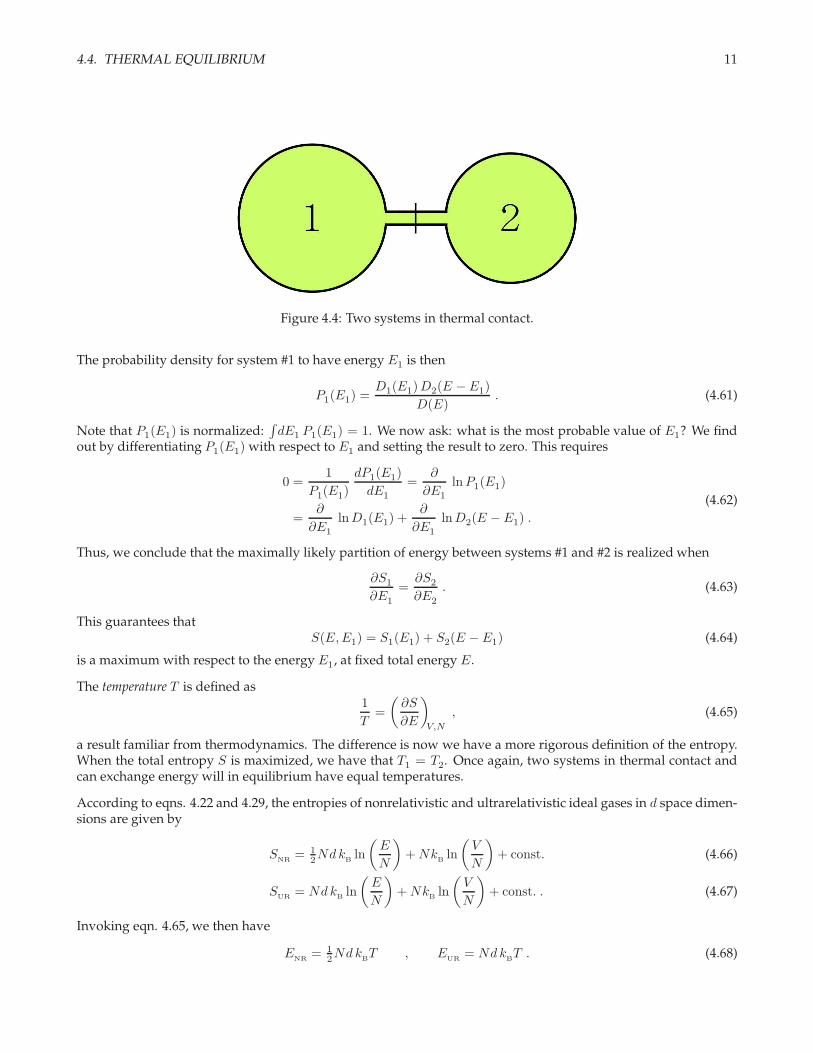
4.4. THERMAL EQUILIBRIUM 11
Figure 4.4: Two systems in thermal contact.
The probability density for system #1 to have energy E1 is then
P1(E1) =D1(E1)D2(E − E1)
D(E). (4.61)
Note that P1(E1) is normalized:∫dE1 P1(E1) = 1. We now ask: what is the most probable value of E1? We find
out by differentiating P1(E1) with respect to E1 and setting the result to zero. This requires
0 =1
P1(E1)
dP1(E1)
dE1
=∂
∂E1
lnP1(E1)
=∂
∂E1
lnD1(E1) +∂
∂E1
lnD2(E − E1) .
(4.62)
Thus, we conclude that the maximally likely partition of energy between systems #1 and #2 is realized when
∂S1
∂E1
=∂S2
∂E2
. (4.63)
This guarantees thatS(E,E1) = S1(E1) + S2(E − E1) (4.64)
is a maximum with respect to the energy E1, at fixed total energy E.
The temperature T is defined as1
T=
(∂S
∂E
)
V,N
, (4.65)
a result familiar from thermodynamics. The difference is now we have a more rigorous definition of the entropy.When the total entropy S is maximized, we have that T1 = T2. Once again, two systems in thermal contact andcan exchange energy will in equilibrium have equal temperatures.
According to eqns. 4.22 and 4.29, the entropies of nonrelativistic and ultrarelativistic ideal gases in d space dimen-sions are given by
SNR
= 12NdkB
ln
(E
N
)+Nk
Bln
(V
N
)+ const. (4.66)
SUR
= NdkB
ln
(E
N
)+Nk
Bln
(V
N
)+ const. . (4.67)
Invoking eqn. 4.65, we then have
ENR
= 12NdkB
T , EUR
= NdkBT . (4.68)
12 CHAPTER 4. STATISTICAL ENSEMBLES
We saw that the probability distribution P1(E1) is maximized when T1 = T2, but how sharp is the peak in thedistribution? Let us write E1 = E∗
1 + ∆E1, where E∗1 is the solution to eqn. 4.62. We then have
lnP1(E∗1 + ∆E1) = lnP1(E
∗1 ) +
1
2kB
∂2S1
∂E21
∣∣∣∣E∗
1
(∆E1)2 +
1
2kB
∂2S2
∂E22
∣∣∣∣E∗
2
(∆E1)2 + . . . , (4.69)
where E∗2 = E − E∗
1 . We must now evaluate
∂2S
∂E2=
∂
∂E
(1
T
)= − 1
T 2
(∂T
∂E
)
V,N
= − 1
T 2CV
, (4.70)
where CV =(∂E/∂T
)V,N
is the heat capacity. Thus,
P1 = P ∗1 e
−(∆E1)2/2kBT 2CV , (4.71)
where
CV =CV,1 CV,2
CV,1 + CV,2
. (4.72)
The distribution is therefore a Gaussian, and the fluctuations in ∆E1 can now be computed:
⟨(∆E1)
2⟩
= kBT 2 CV =⇒ (∆E1)RMS
= kBT√CV /kB
. (4.73)
The individual heat capacities CV,1 and CV,2 scale with the volumes V1 and V2, respectively. If V2 ≫ V1, then
CV,2 ≫ CV,1, in which case CV ≈ CV,1. Therefore the RMS fluctuations in ∆E1 are proportional to the square
root of the system size, whereas E1 itself is extensive. Thus, the ratio (∆E1)RMS/E1 ∝ V −1/2 scales as the inverse
square root of the volume. The distribution P1(E1) is thus extremely sharp.
4.5 Ordinary Canonical Ensemble (OCE)
4.5.1 Canonical distribution and partition function
Consider a system S in contact with a world W , and let their union U = W ∪ S be called the ‘universe’. Thesituation is depicted in fig. 4.2. The volume V
Sand particle number N
Sof the system are held fixed, but the
energy is allowed to fluctuate by exchange with the world W . We are interested in the limit NS→ ∞, N
W→ ∞,
with NS≪ N
W, with similar relations holding for the respective volumes and energies. We now ask what is the
probability that S is in a state |n 〉 with energy En. This is given by the ratio
Pn = lim∆E→0
DW
(EU− En)∆E
DU(E
U)∆E
=# of states accessible to W given that E
S= En
total # of states in U.
(4.74)
Then
lnPn = lnDW
(EU− En) − lnD
U(E
U)
= lnDW
(EU) − lnD
U(E
U) − En
∂ lnDW
(E)
∂E
∣∣∣∣E=E
U
+ . . .
≡ −α− βEn .
(4.75)
4.5. ORDINARY CANONICAL ENSEMBLE (OCE) 13
The constant β is given by
β =∂ lnD
W(E)
∂E
∣∣∣∣E=E
U
=1
kBT. (4.76)
Thus, we find Pn = e−α e−βEn . The constant α is fixed by the requirement that∑
n Pn = 1:
Pn =1
Ze−βEn , Z(T, V,N) =
∑
n
e−βEn = Tr e−βH . (4.77)
We’ve already met Z(β) in eqn. 4.23 – it is the Laplace transform of the density of states. It is also called thepartition function of the system S. Quantum mechanically, we can write the ordinary canonical density matrix as
ˆ =e−βH
Tr e−βH. (4.78)
Note that[ˆ, H
]= 0, hence the ordinary canonical distribution is a stationary solution to the evolution equation
for the density matrix. Note that the OCE is specified by three parameters: T , V , and N .
4.5.2 The difference between P (En) and Pn
Let the total energy of the Universe be fixed at EU
. The joint probability density P (ES, E
W) for the system to have
energy ES and the world to have energy EW
is
P (ES, E
W) = D
S(E
S)D
W(E
W) δ(E
U− E
S− E
W)/D
U(E
U) , (4.79)
where
DU(E
U) =
∞∫
−∞
dESD
S(E
S)D
W(E
U− E
S) , (4.80)
which ensures that∫dE
S
∫dE
WP (E
S, E
W) = 1. The probability density P (E
S) is defined such that P (E
S) dE
Sis
the (differential) probability for the system to have an energy in the range [ES, E
S+ dE
S]. The units of P (E
S) are
E−1. To obtain P (ES), we simply integrate the joint probability density P (E
S, E
W) over all possible values of E
W,
obtaining
P (ES) =
DS(E
S)D
W(E
U− E
S)
DU(E
U)
, (4.81)
as we have in eqn. 4.74.
Now suppose we wish to know the probability Pn that the system is in a particular state |n 〉 with energy En.Clearly
Pn = lim∆E→0
probability that ES∈ [En, En + ∆E]
# of S states with ES∈ [En, En + ∆E]
=P (En)∆E
DS(En)∆E
=D
W(E
U− En)
DU(E
U)
. (4.82)
4.5.3 Averages within the OCE
To compute averages within the OCE,
⟨A⟩
= Tr(ˆA)
=
∑n 〈n|A|n〉 e−βEn
∑n e
−βEn
, (4.83)
14 CHAPTER 4. STATISTICAL ENSEMBLES
where we have conveniently taken the trace in a basis of energy eigenstates. In the classical limit, we have
(ϕ) =1
Ze−βH(ϕ) , Z = Tr e−βH =
∫dµ e−βH(ϕ) , (4.84)
with dµ = 1N !
∏Nj=1(d
dqj ddpj/h
d) for identical particles (‘Maxwell-Boltzmann statistics’). Thus,
〈A〉 = Tr (A) =
∫dµ A(ϕ) e−βH(ϕ)
∫dµ e−βH(ϕ)
. (4.85)
4.5.4 Entropy and free energy
The Boltzmann entropy is defined by
S = −kB
Tr(ˆ ln ˆ) = −k
B
∑
n
Pn lnPn . (4.86)
The Boltzmann entropy and the statistical entropy S = kB
lnD(E) are identical in the thermodynamic limit.
We define the Helmholtz free energy F (T, V,N) as
F (T, V,N) = −kBT lnZ(T, V,N) , (4.87)
hencePn = eβF e−βEn , lnPn = βF − βEn . (4.88)
Therefore the entropy is
S = −kB
∑
n
Pn
(βF − βEn
)
= −FT
+〈 H 〉T
,
(4.89)
which is to sayF = E − TS , (4.90)
where
E =∑
n
PnEn =Tr H e−βH
Tr e−βH(4.91)
is the average energy. We also see that
Z = Tr e−βH =∑
n
e−βEn =⇒ E =
∑nEn e
−βEn
∑n e
−βEn
= − ∂
∂βlnZ =
∂
∂β
(βF). (4.92)
Thus, F (T, V,N) is a Legendre transform of E(S, V,N), with
dF = −S dT − p dV + µdN , (4.93)
which means
S = −(∂F
∂T
)
V,N
, p = −(∂F
∂V
)
T,N
, µ = +
(∂F
∂N
)
T,V
. (4.94)
4.5. ORDINARY CANONICAL ENSEMBLE (OCE) 15
4.5.5 Fluctuations in the OCE
In the OCE, the energy is not fixed. It therefore fluctuates about its average value E = 〈H〉. Note that
−∂E∂β
= kBT 2 ∂E
∂T=∂2 lnZ
∂β2
=Tr H2 e−βH
Tr e−βH−(
Tr H e−βH
Tr e−βH
)2
=⟨H2⟩−⟨H⟩2.
(4.95)
Thus, the heat capacity is related to the fluctuations in the energy, just as we saw at the end of §4.4:
CV =
(∂E
∂T
)
V,N
=1
kBT 2
(⟨H2⟩−⟨H⟩2)
(4.96)
For the nonrelativistic ideal gas, we found CV = d2 NkB
, hence the ratio of RMS fluctuations in the energy to theenergy itself is √⟨
(∆H)2⟩
〈H〉=
√k
BT 2CV
d2NkB
T=
√2
Nd, (4.97)
and the ratio of the RMS fluctuations to the mean value vanishes in the thermodynamic limit.
The full distribution function for the energy is
P (E) =⟨δ(E − H)
⟩=
Tr δ(E − H) e−βH
Tr e−βH=
1
ZD(E) e−βE . (4.98)
Thus,
P (E) =e−β[E−TS(E)]
∫dE e−β[E−TS(E)]
, (4.99)
where S(E) = kB
lnD(E) is the statistical entropy. Let’s write E = E + δE , where E extremizes the combinationE − T S(E), i.e. the solution to T S′(E) = 1, where the energy derivative of S is performed at fixed volume V andparticle number N . We now expand S(E + δE) to second order in δE , obtaining
S(E + δE) = S(E) +δET
−(δE)2
2T 2CV
+ . . . (4.100)
Recall that S′′(E) = ∂∂E
(1T
)= − 1
T 2CV
. Thus,
E − T S(E) = E − T S(E) +(δE)2
2T CV
+ O((δE)2
). (4.101)
Applying this to both numerator and denominator of eqn. 4.99, we obtain4
P (E) = N exp
[− (δE)2
2kBT 2CV
], (4.102)
where N = (2πkBT 2CV )−1/2 is a normalization constant which guarantees
∫dE P (E) = 1. Once again, we see that
the distribution is a Gaussian centered at 〈E〉 = E, and of width (∆E)RMS =√k
BT 2CV . This is a consequence of
the Central Limit Theorem.4In applying eqn. 4.101 to the denominator of eqn. 4.99, we shift E by E and integrate over the difference δE ≡ E − E, retaining terms up
to quadratic order in δE in the argument of the exponent.
16 CHAPTER 4. STATISTICAL ENSEMBLES
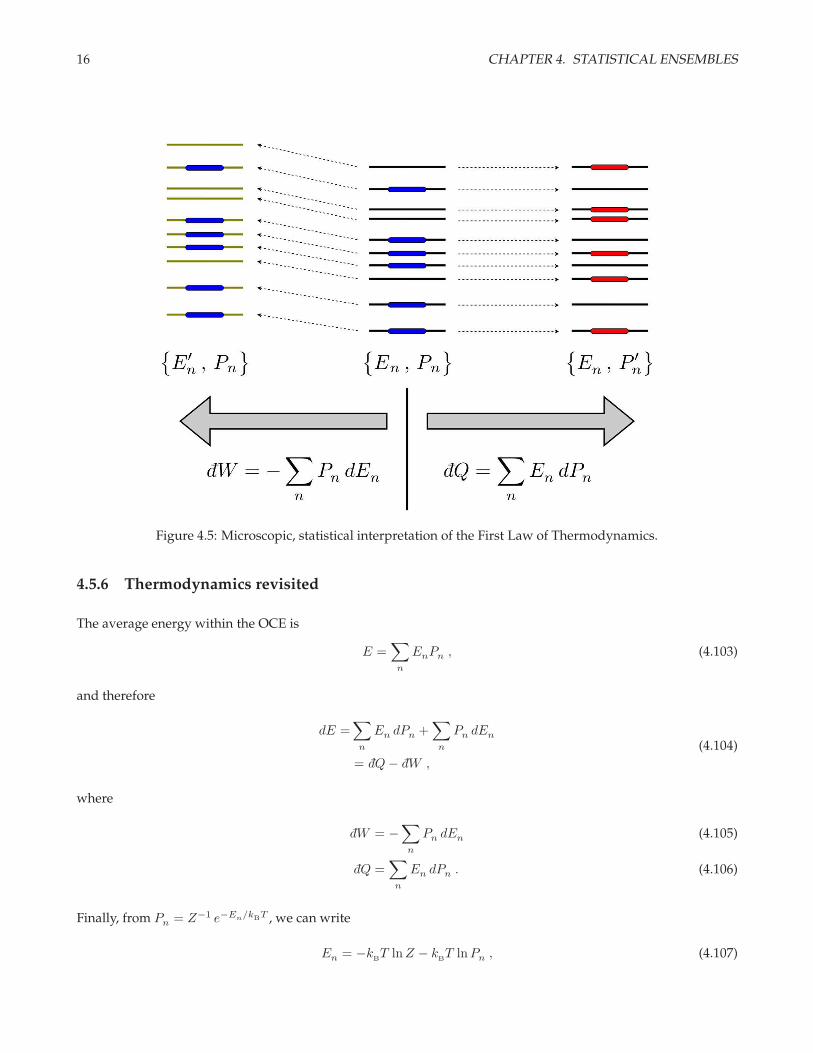
Figure 4.5: Microscopic, statistical interpretation of the First Law of Thermodynamics.
4.5.6 Thermodynamics revisited
The average energy within the OCE is
E =∑
n
EnPn , (4.103)
and therefore
dE =∑
n
En dPn +∑
n
Pn dEn
= dQ− dW ,
(4.104)
where
dW = −∑
n
Pn dEn (4.105)
dQ =∑
n
En dPn . (4.106)
Finally, from Pn = Z−1 e−En/kBT , we can write
En = −kBT lnZ − k
BT lnPn , (4.107)
4.5. ORDINARY CANONICAL ENSEMBLE (OCE) 17
with which we obtain
dQ =∑
n
En dPn
= −kBT lnZ
∑
n
dPn − kBT∑
n
lnPn dPn
= T d(− k
B
∑
n
Pn lnPn
)= T dS .
(4.108)
Note also that
dW = −∑
n
Pn dEn
= −∑
n
Pn
(∑
i
∂En
∂Xi
dXi
)
= −∑
n,i
Pn
⟨n∣∣ ∂H∂Xi
∣∣n⟩dXi ≡
∑
i
Fi dXi ,
(4.109)
so the generalized force Fi conjugate to the generalized displacement dXi is
Fi = −∑
n
Pn
∂En
∂Xi
= −⟨∂H
∂Xi
⟩. (4.110)
This is the force acting on the system5. In the chapter on thermodynamics, we defined the generalized forceconjugate to Xi as yi ≡ −Fi.
Thus we see from eqn. 4.104 that there are two ways that the average energy can change; these are depicted inthe sketch of fig. 4.5. Starting from a set of energy levels En and probabilities Pn, we can shift the energiesto E′
n. The resulting change in energy (∆E)I= −W is identified with the work done on the system. We could
also modify the probabilities to P ′n without changing the energies. The energy change in this case is the heat
absorbed by the system: (∆E)II
= Q. This provides us with a statistical and microscopic interpretation of the FirstLaw of Thermodynamics.
4.5.7 Generalized susceptibilities
Suppose our Hamiltonian is of the form
H = H(λ) = H0 − λ Q , (4.111)
where λ is an intensive parameter, such as magnetic field. Then
Z(λ) = Tr e−β(H0−λQ) (4.112)
and1
Z
∂Z
∂λ= β · 1
ZTr
(Q e−βH(λ)
)= β 〈Q〉 . (4.113)
But then from Z = e−βF we have
Q(λ, T ) = 〈 Q 〉 = −(∂F
∂λ
)
T
. (4.114)
5In deriving eqn. 4.110, we have used the so-called Feynman-Hellman theorem of quantum mechanics: d〈n|H|n〉 = 〈n| dH |n〉, if |n〉 is anenergy eigenstate.
18 CHAPTER 4. STATISTICAL ENSEMBLES
Typically we will take Q to be an extensive quantity. We can now define the susceptibility χ as
χ =1
V
∂Q
∂λ= − 1
V
∂2F
∂λ2. (4.115)
The volume factor in the denominator ensures that χ is intensive.
It is important to realize that we have assumed here that[H0 , Q
]= 0, i.e. the ‘bare’ Hamiltonian H0 and the
operator Q commute. If they do not commute, then the response functions must be computed within a properquantum mechanical formalism, which we shall not discuss here.
Note also that we can imagine an entire family of observablesQk
satisfying
[Qk , Qk′
]= 0 and
[H0 , Qk
]= 0,
for all k and k′. Then for the Hamiltonian
H (~λ) = H0 −∑
k
λk Qk , (4.116)
we have that
Qk(~λ, T ) = 〈 Qk 〉 = −(∂F
∂λk
)
T, Na, λk′ 6=k
(4.117)
and we may define an entire matrix of susceptibilities,
χkl =
1
V
∂Qk
∂λl
= − 1
V
∂2F
∂λk ∂λl
. (4.118)
4.6 Grand Canonical Ensemble (GCE)
4.6.1 Grand canonical distribution and partition function
Consider once again the situation depicted in fig. 4.2, where a system S is in contact with a world W , their unionU = W ∪S being called the ‘universe’. We assume that the system’s volume V
Sis fixed, but otherwise it is allowed
to exchange energy and particle number with W . Hence, the system’s energy ES
and particle number NS
willfluctuate. We ask what is the probability that S is in a state |n 〉 with energy En and particle number Nn. This isgiven by the ratio
Pn = lim∆E→0
DW
(EU− En , NU
−Nn)∆E
DU(E
U, N
U)∆E
=# of states accessible to W given that E
S= En and N
S= Nn
total # of states in U.
(4.119)
Then
lnPn = lnDW
(EU− En , NU
−Nn) − lnDU(E
U, N
U)
= lnDW
(EU, N
U) − lnD
U(E
U, N
U)
− En
∂ lnDW
(E,N)
∂E
∣∣∣∣E=E
UN=N
U
−Nn
∂ lnDW
(E,N)
∂N
∣∣∣∣E=E
UN=N
U
+ . . .
≡ −α− βEn + βµNn .
(4.120)
4.6. GRAND CANONICAL ENSEMBLE (GCE) 19
The constants β and µ are given by
β =∂ lnD
W(E,N)
∂E
∣∣∣∣ E=EU
N=NU
=1
kBT
(4.121)
µ = −kBT∂ lnD
W(E,N)
∂N
∣∣∣∣ E=EU
N=NU
. (4.122)
The quantity µ has dimensions of energy and is called the chemical potential. Nota bene: Some texts define the
‘grand canonical Hamiltonian’ K as
K ≡ H − µN . (4.123)
Thus, Pn = e−α e−β(En−µNn). Once again, the constant α is fixed by the requirement that∑
n Pn = 1:
Pn =1
Ξe−β(En−µNn) , Ξ(β, V, µ) =
∑
n
e−β(En−µNn) = Tr e−β(H−µN) = Tr e−βK . (4.124)
Thus, the quantum mechanical grand canonical density matrix is given by
ˆ =e−βK
Tr e−βK. (4.125)
Note that[ˆ, K
]= 0.
The quantity Ξ(T, V, µ) is called the grand partition function. It stands in relation to a corresponding free energy inthe usual way:
Ξ(T, V, µ) ≡ e−βΩ(T,V,µ) ⇐⇒ Ω = −kBT ln Ξ , (4.126)
where Ω(T, V, µ) is the grand potential, also known as the Landau free energy. The dimensionless quantity z ≡ eβµ
is called the fugacity.
If[H, N
]= 0, the grand potential may be expressed as a sum over contributions from each N sector, viz.
Ξ(T, V, µ) =∑
N
eβµN Z(T, V,N) . (4.127)
When there is more than one species, we have several chemical potentials µa, and accordingly we define
K = H −∑
a
µa Na , (4.128)
with Ξ = Tr e−βK as before.
4.6.2 Entropy and Gibbs-Duhem relation
In the GCE, the Boltzmann entropy is
S = −kB
∑
n
Pn lnPn
= −kB
∑
n
Pn
(βΩ − βEn + βµNn
)
= −ΩT
+〈H〉T
− µ 〈N〉T
,
(4.129)
20 CHAPTER 4. STATISTICAL ENSEMBLES
which saysΩ = E − TS − µN , (4.130)
where
E =∑
n
En Pn = Tr(ˆH)
(4.131)
N =∑
n
Nn Pn = Tr(ˆN). (4.132)
Therefore, Ω(T, V, µ) is a double Legendre transform of E(S, V,N), with
dΩ = −S dT − p dV −N dµ , (4.133)
which entails
S = −(∂Ω
∂T
)
V,µ
, p = −(∂Ω
∂V
)
T,µ
, N = −(∂Ω
∂µ
)
T,V
. (4.134)
Since Ω(T, V, µ) is an extensive quantity, we must be able to write Ω = V ω(T, µ). We identify the function ω(T, µ)as the negative of the pressure:
∂Ω
∂V= −kB
T
Ξ
(∂Ξ
∂V
)
T,µ
=1
Ξ
∑
n
∂En
∂Ve−β(En−µNn)
=
(∂E
∂V
)
T,µ
= −p(T, µ) .
(4.135)
Therefore,Ω = −pV , p = p(T, µ) (equation of state) . (4.136)
This is consistent with the result from thermodynamics that G = E − TS + pV = µN . Taking the differential, weobtain the Gibbs-Duhem relation,
dΩ = −S dT − p dV −N dµ = −p dV − V dp ⇒ S dT − V dp+N dµ = 0 . (4.137)
4.6.3 Generalized susceptibilities in the GCE
We can appropriate the results from §4.5.7 and apply them, mutatis mutandis, to the GCE. Suppose we have a
family of observablesQk
satisfying
[Qk , Qk′
]= 0 and
[H0 , Qk
]= 0 and
[Na , Qk
]= 0 for all k, k′, and a.
Then for the grand canonical Hamiltonian
K (~λ) = H0 −∑
a
µa Na −∑
k
λk Qk , (4.138)
we have that
Qk(~λ, T ) = 〈 Qk 〉 = −(∂Ω
∂λk
)
T,µa, λk′ 6=k
(4.139)
and we may define the matrix of generalized susceptibilities,
χkl =
1
V
∂Qk
∂λl
= − 1
V
∂2Ω
∂λk ∂λl
. (4.140)
4.6. GRAND CANONICAL ENSEMBLE (GCE) 21
4.6.4 Fluctuations in the GCE
Both energy and particle number fluctuate in the GCE. Let us compute the fluctuations in particle number. Wehave
N = 〈 N 〉 =Tr N e−β(H−µN)
Tr e−β(H−µN)=
1
β
∂
∂µln Ξ . (4.141)
Therefore,
1
β
∂N
∂µ=
Tr N2 e−β(H−µN)
Tr e−β(H−µN)−(
Tr N e−β(H−µN)
Tr e−β(H−µN)
)2
=⟨N2⟩−⟨N⟩2.
(4.142)
Note now that ⟨N2⟩−⟨N⟩2
⟨N⟩2 =
kBT
N2
(∂N
∂µ
)
T,V
=k
BT
VκT , (4.143)
where κT is the isothermal compressibility. Note:(∂N
∂µ
)
T,V
=∂(N,T, V )
∂(µ, T, V )
=∂(N,T, V )
∂(N,T, p)· ∂(N,T, p)
∂(V, T, p)·
1︷ ︸︸ ︷∂(V, T, p)
∂(N,T, µ)·∂(N,T, µ)
∂(V, T, µ)
= −N2
V 2
(∂V
∂p
)
T,N
=N2
VκT .
(4.144)
Thus,(∆N)
RMS
N=
√k
BT κT
V, (4.145)
which again scales as V −1/2.
4.6.5 Gibbs ensemble
Let the system’s particle number N be fixed, but let it exchange energy and volume with the world W . Mutatismutandis, we have
Pn = lim∆E→0
lim∆V →0
DW
(EU− En , VU
− Vn)∆E∆V
DU(E
U, V
U)∆E∆V
. (4.146)
Then
lnPn = lnDW
(EU− En , VU
− Vn) − lnDU(E
U, V
U)
= lnDW
(EU, V
U) − lnD
U(E
U, V
U)
− En
∂ lnDW
(E, V )
∂E
∣∣∣∣E=E
UV =V
U
− Vn∂ lnD
W(E, V )
∂V
∣∣∣∣E=E
UV =V
U
+ . . .
≡ −α− βEn − βp Vn .
(4.147)
22 CHAPTER 4. STATISTICAL ENSEMBLES
The constants β and p are given by
β =∂ lnD
W(E, V )
∂E
∣∣∣∣E=EU
V =VU
=1
kBT
(4.148)
p = kBT∂ lnD
W(E, V )
∂V
∣∣∣∣E=E
UV =V
U
. (4.149)
The corresponding partition function is
Y (T, p,N) = Tr e−β(H+pV ) =1
V0
∞∫
0
dV e−βpV Z(T, V,N) ≡ e−βG(T,p,N) , (4.150)
where V0 is a constant which has dimensions of volume. The factor V −10 in front of the integral renders Y di-
mensionless. Note that G(V ′0) = G(V0) + k
BT ln(V ′
0/V0), so the difference is not extensive and can be neglectedin the thermodynamic limit. In other words, it doesn’t matter what constant we choose for V0 since it contributessubextensively to G. Moreover, in computing averages, the constant V0 divides out in the ratio of numeratorand denominator. Like the Helmholtz free energy, the Gibbs free energy G(T, p,N) is also a double Legendretransform of the energy E(S, V,N), viz.
G = E − TS + pV
dG = −S dT + V dp+ µdN ,(4.151)
which entails
S = −(∂G
∂T
)
p,N
, V = +
(∂G
∂p
)
T,N
, µ = +
(∂G
∂N
)
T,p
. (4.152)
4.7 Statistical Ensembles from Maximum Entropy
The basic principle: maximize the entropy,
S = −kB
∑
n
Pn lnPn . (4.153)
4.7.1 µCE
We maximize S subject to the single constraint
C =∑
n
Pn − 1 = 0 . (4.154)
We implement the constraint C = 0 with a Lagrange multiplier, λ ≡ kBλ, writing
S∗ = S − kBλC , (4.155)
and freely extremizing over the distribution Pn and the Lagrange multiplier λ. Thus,
δS∗ = δS − kBλ δC − k
BC δλ
= −kB
∑
n
[lnPn + 1 + λ
]δPn − k
BC δλ ≡ 0 . (4.156)
4.7. STATISTICAL ENSEMBLES FROM MAXIMUM ENTROPY 23
We conclude that C = 0 and thatlnPn = −
(1 + λ
), (4.157)
and we fix λ by the normalization condition∑
n Pn = 1. This gives
Pn =1
Ω, Ω =
∑
n
Θ(E + ∆E − En)Θ(En − E) . (4.158)
Note that Ω is the number of states with energies between E and E + ∆E.
4.7.2 OCE
We maximize S subject to the two constraints
C1 =∑
n
Pn − 1 = 0 , C2 =∑
n
En Pn − E = 0 . (4.159)
We now have two Lagrange multipliers. We write
S∗ = S − kB
2∑
j=1
λj Cj , (4.160)
and we freely extremize over Pn and Cj. We therefore have
δS∗ = δS − kB
∑
n
(λ1 + λ2En
)δPn − k
B
2∑
j=1
Cj δλj
= −kB
∑
n
[lnPn + 1 + λ1 + λ2 En
]δPn − k
B
2∑
j=1
Cj δλj ≡ 0 .
(4.161)
Thus, C1 = C2 = 0 andlnPn = −
(1 + λ1 + λ2En
). (4.162)
We define λ2 ≡ β and we fix λ1 by normalization. This yields
Pn =1
Ze−βEn , Z =
∑
n
e−βEn . (4.163)
4.7.3 GCE
We maximize S subject to the three constraints
C1 =∑
n
Pn − 1 = 0 , C2 =∑
n
En Pn − E = 0 , C3 =∑
n
Nn Pn −N = 0 . (4.164)
We now have three Lagrange multipliers. We write
S∗ = S − kB
3∑
j=1
λj Cj , (4.165)
24 CHAPTER 4. STATISTICAL ENSEMBLES
and hence
δS∗ = δS − kB
∑
n
(λ1 + λ2 En + λ3Nn
)δPn − k
B
3∑
j=1
Cj δλj
= −kB
∑
n
[lnPn + 1 + λ1 + λ2En + λ3Nn
]δPn − k
B
3∑
j=1
Cj δλj ≡ 0 .
(4.166)
Thus, C1 = C2 = C3 = 0 andlnPn = −
(1 + λ1 + λ2 En + λ3Nn
). (4.167)
We define λ2 ≡ β and λ3 ≡ −βµ, and we fix λ1 by normalization. This yields
Pn =1
Ξe−β(En−µNn) , Ξ =
∑
n
e−β(En−µNn) . (4.168)
4.8 Ideal Gas Statistical Mechanics
The ordinary canonical partition function for the ideal gas was computed in eqn. 4.25. We found
Z(T, V,N) =1
N !
N∏
i=1
∫ddxi d
dpi
(2π~)de−βp2
i /2m
=V N
N !
∞∫
−∞
dp
2π~e−βp2/2m
Nd
=1
N !
(V
λdT
)N
,
(4.169)
where λT is the thermal wavelength:
λT =√
2π~2/mkBT . (4.170)
The physical interpretation of λT is that it is the de Broglie wavelength for a particle of mass mwhich has a kineticenergy of k
BT .
In the GCE, we have
Ξ(T, V, µ) =
∞∑
N=0
eβµN Z(T, V,N)
=
∞∑
N=1
1
N !
(V eµ/kBT
λdT
)N
= exp
(V eµ/kBT
λdT
).
(4.171)
From Ξ = e−Ω/kBT , we have the grand potential is
Ω(T, V, µ) = −V kBT eµ/kBT
/λd
T . (4.172)
Since Ω = −pV (see §4.6.2), we havep(T, µ) = k
BT λ−d
T eµ/kBT . (4.173)
The number density can also be calculated:
n =N
V= − 1
V
(∂Ω
∂µ
)
T,V
= λ−dT eµ/kBT . (4.174)
Combined, the last two equations recapitulate the ideal gas law, pV = NkBT .
4.8. IDEAL GAS STATISTICAL MECHANICS 25
4.8.1 Maxwell velocity distribution
The distribution function for momenta is given by
g(p) =⟨ 1
N
N∑
i=1
δ(pi − p)⟩. (4.175)
Note that g(p) =⟨δ(pi − p)
⟩is the same for every particle, independent of its label i. We compute the average
〈A〉 = Tr(Ae−βH
)/Tr e−βH . Setting i = 1, all the integrals other than that over p1 divide out between numerator
and denominator. We then have
g(p) =
∫d3p1 δ(p1 − p) e−βp2
1/2m
∫d3p1 e
−βp21/2m
= (2πmkBT )−3/2 e−βp2/2m .
(4.176)
Textbooks commonly refer to the velocity distribution f(v), which is related to g(p) by
f(v) d3v = g(p) d3p . (4.177)
Hence,
f(v) =
(m
2πkBT
)3/2
e−mv2/2kBT . (4.178)
This is known as the Maxwell velocity distribution. Note that the distributions are normalized, viz.∫d3p g(p) =
∫d3v f(v) = 1 . (4.179)
If we are only interested in averaging functions of v = |v| which are isotropic, then we can define the Maxwell
speed distribution, f(v), as
f(v) = 4π v2f(v) = 4π
(m
2πkBT
)3/2
v2 e−mv2/2kBT . (4.180)
Note that f(v) is normalized according to∞∫
0
dv f(v) = 1 . (4.181)
It is convenient to represent v in units of v0 =√k
BT/m, in which case
f(v) =1
v0ϕ(v/v0) , ϕ(s) =
√2π s
2 e−s2/2 . (4.182)
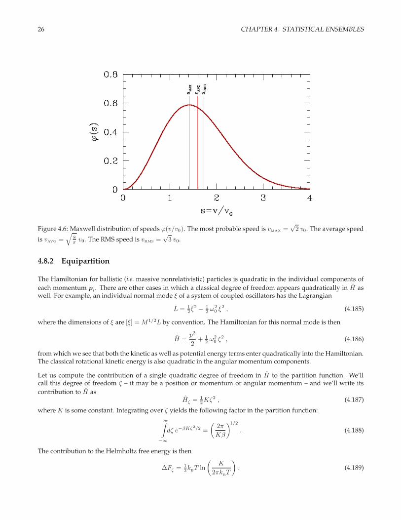
The distribution ϕ(s) is shown in fig. 4.6. Computing averages, we have
Ck ≡ 〈sk〉 =
∞∫
0
ds sk ϕ(s) = 2k/2 · 2√π
Γ(
32 + k
2
). (4.183)
Thus, C0 = 1, C1 =√
8π , C2 = 3, etc. The speed averages are
⟨vk⟩
= Ck
(k
BT
m
)k/2
. (4.184)
Note that the average velocity is 〈v〉 = 0, but the average speed is 〈v〉 =√
8kBT/πm. The speed distribution is
plotted in fig. 4.6.
26 CHAPTER 4. STATISTICAL ENSEMBLES
Figure 4.6: Maxwell distribution of speeds ϕ(v/v0). The most probable speed is vMAX =√
2 v0. The average speed
is vAVG =√
8π v0. The RMS speed is vRMS =
√3 v0.
4.8.2 Equipartition
The Hamiltonian for ballistic (i.e. massive nonrelativistic) particles is quadratic in the individual components of
each momentum pi. There are other cases in which a classical degree of freedom appears quadratically in H aswell. For example, an individual normal mode ξ of a system of coupled oscillators has the Lagrangian
L = 12 ξ
2 − 12 ω
20 ξ
2 , (4.185)
where the dimensions of ξ are [ξ] = M1/2L by convention. The Hamiltonian for this normal mode is then
H =p2
2+ 1
2 ω20 ξ
2 , (4.186)
from which we see that both the kinetic as well as potential energy terms enter quadratically into the Hamiltonian.The classical rotational kinetic energy is also quadratic in the angular momentum components.
Let us compute the contribution of a single quadratic degree of freedom in H to the partition function. We’llcall this degree of freedom ζ – it may be a position or momentum or angular momentum – and we’ll write its
contribution to H asHζ = 1
2Kζ2 , (4.187)
where K is some constant. Integrating over ζ yields the following factor in the partition function:
∞∫
−∞
dζ e−βKζ2/2 =
(2π
Kβ
)1/2
. (4.188)
The contribution to the Helmholtz free energy is then
∆Fζ = 12kB
T ln
(K
2πkBT
), (4.189)
4.8. IDEAL GAS STATISTICAL MECHANICS 27
and therefore the contribution to the internal energy E is
∆Eζ =∂
∂β
(β∆Fζ
)=
1
2β= 1
2kBT . (4.190)
We have thus derived what is commonly called the equipartition theorem of classical statistical mechanics:
To each degree of freedom which enters the Hamiltonian quadratically is associated a contribution12kB
T to the internal energy of the system. This results in a concomitant contribution of 12kB
to the heatcapacity.
We now see why the internal energy of a classical ideal gas with f degrees of freedom per molecule is E =12fNkB
T , and CV = 12NkB
. This result also has applications in the theory of solids. The atoms in a solid possesskinetic energy due to their motion, and potential energy due to the spring-like interatomic potentials which tendto keep the atoms in their preferred crystalline positions. Thus, for a three-dimensional crystal, there are sixquadratic degrees of freedom (three positions and three momenta) per atom, and the classical energy shouldbe E = 3Nk
BT , and the heat capacity CV = 3Nk
B. As we shall see, quantum mechanics modifies this result
considerably at temperatures below the highest normal mode (i.e. phonon) frequency, but the high temperaturelimit is given by the classical value CV = 3νR (where ν = N/NA is the number of moles) derived here, known asthe Dulong-Petit limit.
4.8.3 Quantum statistics and the Maxwell-Boltzmann limit
Consider a system composed of N noninteracting particles. The Hamiltonian is
H =
N∑
j=1
hj . (4.191)
The single particle Hamiltonian h has eigenstates |α 〉 with corresponding energy eigenvalues εα. What is thepartition function? Is it
H?
=∑
α1
· · ·∑
αN
e−β(ε
α1+ ε
α2+ ... + ε
αN
)= ζN , (4.192)
where ζ is the single particle partition function,
ζ =∑
α
e−βεα . (4.193)
For systems where the individual particles are distinguishable, such as spins on a lattice which have fixed positions,this is indeed correct. But for particles free to move in a gas, this equation is wrong. The reason is that forindistinguishable particles the many particle quantum mechanical states are specified by a collection of occupationnumbers nα, which tell us how many particles are in the single-particle state |α 〉. The energy is
E =∑
α
nα εα (4.194)
and the total number of particles is
N =∑
α
nα . (4.195)
28 CHAPTER 4. STATISTICAL ENSEMBLES
That is, each collection of occupation numbers nα labels a unique many particle state∣∣ nα
⟩. In the product
ζN , the collection nα occurs many times. We have therefore overcounted the contribution to ZN due to this state.By what factor have we overcounted? It is easy to see that the overcounting factor is
degree of overcounting =N !∏α nα!
,
which is the number of ways we can rearrange the labels αj to arrive at the same collection nα. This followsfrom the multinomial theorem,
(K∑
α=1
xα
)N
=∑
n1
∑
n2
· · ·∑
nK
N !
n1!n2! · · ·nK !x
n1
1 xn2
2 · · ·xnK
K δN,n1 + ...+ nK. (4.196)
Thus, the correct expression for ZN is
ZN =∑
nα
e−βP
αnαεα δN,
Pα
nα
=∑
α1
∑
α2
· · ·∑
αN
(∏α nα!
N !
)e−β(εα
1+ εα
2+ ... + εα
N).
(4.197)
When we study quantum statistics, we shall learn how to handle these constrained sums. For now it suffices tonote that in the high temperature limit, almost all the nα are either 0 or 1, hence
ZN ≈ ζN
N !. (4.198)
This is the classical Maxwell-Boltzmann limit of quantum statistical mechanics. We now see the origin of the 1/N !term which is so important in the thermodynamics of entropy of mixing.
4.9 Selected Examples
4.9.1 Spins in an external magnetic field
Consider a system of Ns spins , each of which can be either up (σ = +1) or down (σ = −1). The Hamiltonian forthis system is
H = −µ0H
Ns∑
j=1
σj , (4.199)
where now we write H for the Hamiltonian, to distinguish it from the external magnetic field H , and µ0 is themagnetic moment per particle. We treat this system within the ordinary canonical ensemble. The partition func-tion is
Z =∑
σ1
· · ·∑
σN
s
e−βH = ζNs , (4.200)
where ζ is the single particle partition function:
ζ =∑
σ=±1
eµ0Hσ/kBT = 2 cosh
(µ0H
kBT
). (4.201)
4.9. SELECTED EXAMPLES 29
The Helmholtz free energy is then
F (T,H,Ns) = −k
BT lnZ = −N
sk
BT ln
[2 cosh
(µ0H
kBT
)]. (4.202)
The magnetization is
M = −(∂F
∂H
)
T, Ns
= Ns µ0 tanh
(µ0H
kBT
). (4.203)
The energy is
E =∂
∂β
(βF)
= −Nsµ0H tanh
(µ0H
kBT
). (4.204)
Hence, E = −HM , which we already knew, from the form of H itself.
Each spin here is independent. The probability that a given spin has polarization σ is
Pσ =eβµ0Hσ
eβµ0H + e−βµ0H. (4.205)
The total probability is unity, and the average polarization is a weighted average of σ = +1 and σ = −1 contribu-tions:
P↑ + P↓ = 1 , 〈σ〉 = P↑ − P↓ = tanh
(µ0H
kBT
). (4.206)
At low temperatures T ≪ µ0H/kB, we have P↑ ≈ 1 − e−2µ0H/kBT . At high temperatures T > µ0H/kB
, the two
polarizations are equally likely, and Pσ ≈ 12
(1 +
σµ0HkB
T
).
The isothermal magnetic susceptibility is defined as
χT =
1
Ns
(∂M
∂H
)
T
=µ2
0
kBT
sech2
(µ0H
kBT
). (4.207)
(Typically this is computed per unit volume rather than per particle.) At H = 0, we have χT = µ20/kB
T , which isknown as the Curie law.
Aside
The energy E = −HM here is not the same quantity we discussed in our study of thermodynamics. In fact,the thermodynamic energy for this problem vanishes! Here is why. To avoid confusion, we’ll need to invoke anew symbol for the thermodynamic energy, E . Recall that the thermodynamic energy E is a function of exten-sive quantities, meaning E = E(S,M,N
s). It is obtained from the free energy F (T,H,N
s) by a double Legendre
transform:
E(S,M,Ns) = F (T,H,Ns) + TS +HM . (4.208)
Now from eqn. 4.202 we derive the entropy
S = −∂F∂T
= Nsk
Bln
[2 cosh
(µ0H
kBT
)]−N
s
µ0H
Ttanh
(µ0H
kBT
). (4.209)
Thus, using eqns. 4.202 and 4.203, we obtain E(S,M,Ns) = 0.
30 CHAPTER 4. STATISTICAL ENSEMBLES
The potential confusion here arises from our use of the expression F (T,H,Ns). In thermodynamics, it is the Gibbs
free energy G(T, p,N) which is a double Legendre transform of the energy: G = E − TS + pV . By analogy, withmagnetic systems we should perhaps write G = E − TS − HM , but in keeping with many textbooks we shalluse the symbol F and refer to it as the Helmholtz free energy. The quantity we’ve called E in eqn. 4.204 is in factE = E −HM , which means E = 0. The energy E(S,M,Ns) vanishes here because the spins are noninteracting.
4.9.2 Negative temperature (!)
Consider again a system of Ns
spins, each of which can be either up (+) or down (−). Let Nσ be the number ofsites with spin σ, where σ = ±1. Clearly N+ + N− = N
s. We now treat this system within the microcanonical
ensemble.
The energy of the system is
E = −HM , (4.210)
where H is an external magnetic field, and M = (N+ −N−)µ0 is the total magnetization. We now compute S(E)using the ordinary canonical ensemble. The number of ways of arranging the system with N+ up spins is
Ω =
(N
s
N+
), (4.211)
hence the entropy is
S = kB
ln Ω = −Ns kB
x ln x+ (1 − x) ln(1 − x)
(4.212)
in the thermodynamic limit: Ns → ∞, N+ → ∞, x = N+/Ns constant. Now the magnetization is M = (N+ −N−)µ0 = (2N+ −N
s)µ0, hence if we define the maximum energy E0 ≡ N
sµ0H , then
E
E0
= − M
Ns µ0
= 1 − 2x =⇒ x =E0 − E
2E0
. (4.213)
We therefore have
S(E,Ns) = −Ns kB
[(E0 − E
2E0
)ln
(E0 − E
2E0
)+
(E0 + E
2E0
)ln
(E0 + E
2E0
)]. (4.214)
We now have
1
T=
(∂S
∂E
)
Ns
=∂S
∂x
∂x
∂E=Ns kB
2E0
ln
(E0 − E
E0 + E
). (4.215)
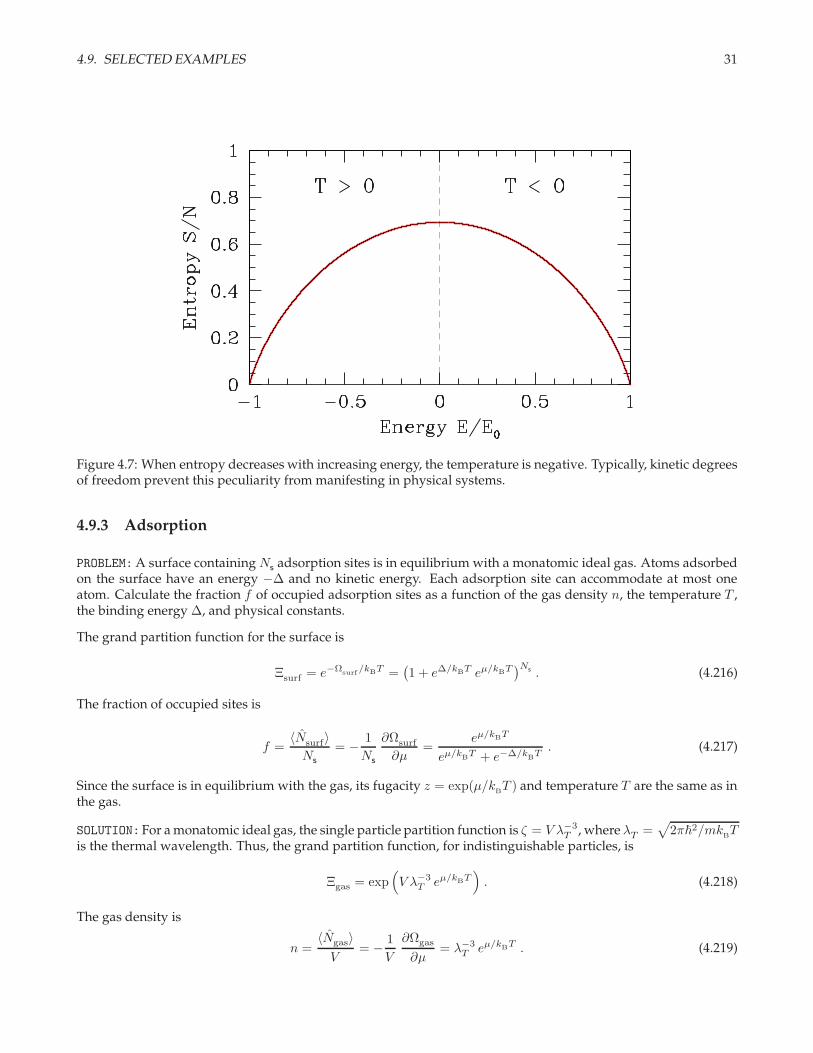
We see that the temperature is positive for −E0 ≤ E < 0 and is negative for 0 < E ≤ E0.
What has gone wrong? The answer is that nothing has gone wrong – all our calculations are perfectly correct. Thissystem does exhibit the possibility of negative temperature. It is, however, unphysical in that we have neglectedkinetic degrees of freedom, which result in an entropy function S(E,N
s) which is an increasing function of energy.
In this system, S(E,Ns) achieves a maximum of Smax = N
sk
Bln 2 at E = 0 (i.e. x = 1
2 ), and then turns over andstarts decreasing. In fact, our results are completely consistent with eqn. 4.204 : the energy E is an odd functionof temperature. Positive energy requires negative temperature! Another example of this peculiarity is providedin the appendix in §4.11.2.
4.9. SELECTED EXAMPLES 31
Figure 4.7: When entropy decreases with increasing energy, the temperature is negative. Typically, kinetic degreesof freedom prevent this peculiarity from manifesting in physical systems.
4.9.3 Adsorption
PROBLEM: A surface containing Ns adsorption sites is in equilibrium with a monatomic ideal gas. Atoms adsorbedon the surface have an energy −∆ and no kinetic energy. Each adsorption site can accommodate at most oneatom. Calculate the fraction f of occupied adsorption sites as a function of the gas density n, the temperature T ,the binding energy ∆, and physical constants.
The grand partition function for the surface is
Ξsurf = e−Ωsurf
/kBT =(1 + e∆/kBT eµ/kBT
)Ns . (4.216)
The fraction of occupied sites is
f =〈Nsurf〉Ns
= − 1
Ns
∂Ωsurf
∂µ=
eµ/kBT
eµ/kB
T + e−∆/kB
T. (4.217)
Since the surface is in equilibrium with the gas, its fugacity z = exp(µ/kBT ) and temperature T are the same as in
the gas.
SOLUTION:For a monatomic ideal gas, the single particle partition function is ζ = V λ−3T , where λT =
√2π~2/mk
BT
is the thermal wavelength. Thus, the grand partition function, for indistinguishable particles, is
Ξgas = exp(V λ−3
T eµ/kBT). (4.218)
The gas density is
n =〈Ngas〉V
= − 1
V
∂Ωgas
∂µ= λ−3
T eµ/kBT . (4.219)
32 CHAPTER 4. STATISTICAL ENSEMBLES
We can now solve for the fugacity: z = eµ/kBT = nλ3T . Thus, the fraction of occupied adsorption sites is
f =nλ3
T
nλ3T + e−∆/k
BT. (4.220)
Interestingly, the solution for f involves the constant ~.
It is always advisable to check that the solution makes sense in various limits. First of all, if the gas density tendsto zero at fixed T and ∆, we have f → 0. On the other hand, if n→ ∞ we have f → 1, which also makes sense. Atfixed n and T , if the adsorption energy is (−∆) → −∞, then once again f = 1 since every adsorption site wants tobe occupied. Conversely, taking (−∆) → +∞ results in n → 0, since the energetic cost of adsorption is infinitelyhigh.
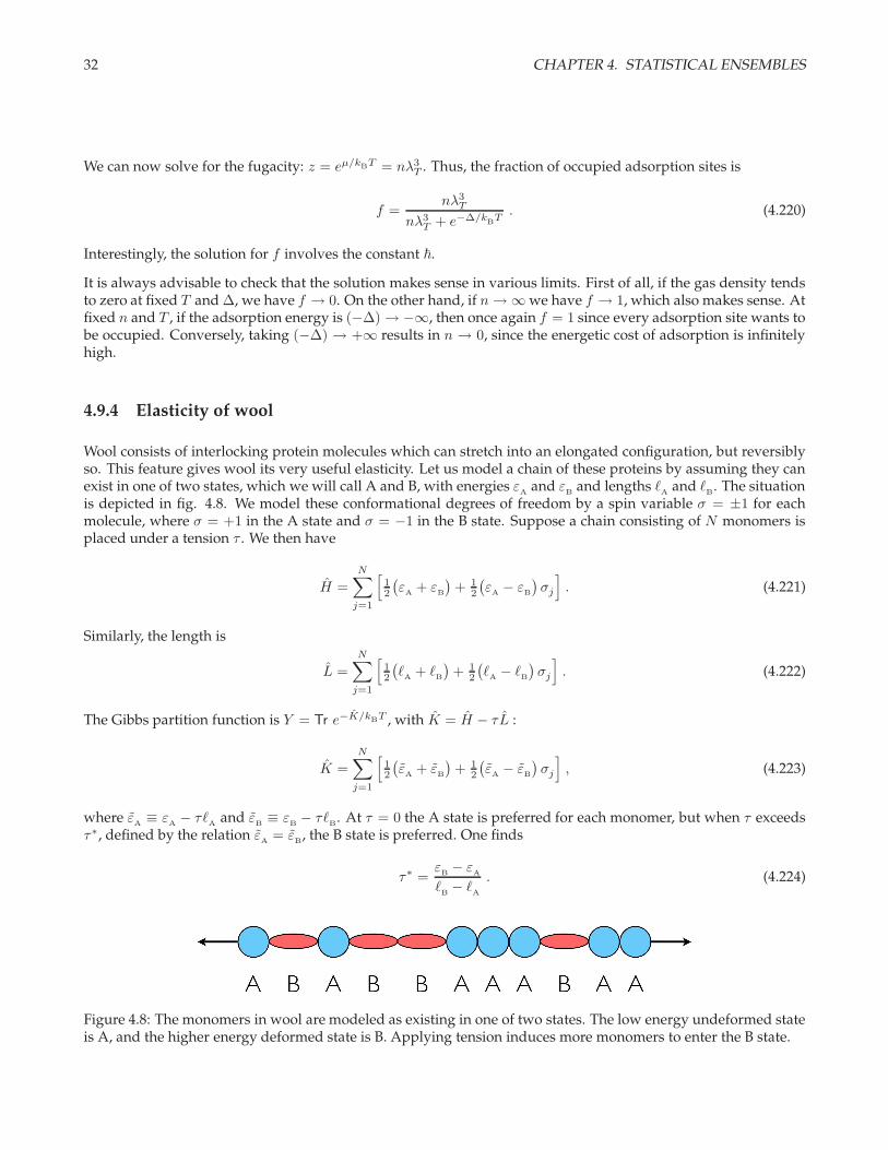
4.9.4 Elasticity of wool
Wool consists of interlocking protein molecules which can stretch into an elongated configuration, but reversiblyso. This feature gives wool its very useful elasticity. Let us model a chain of these proteins by assuming they canexist in one of two states, which we will call A and B, with energies ε
Aand ε
Band lengths ℓ
Aand ℓ
B. The situation
is depicted in fig. 4.8. We model these conformational degrees of freedom by a spin variable σ = ±1 for eachmolecule, where σ = +1 in the A state and σ = −1 in the B state. Suppose a chain consisting of N monomers isplaced under a tension τ . We then have
H =
N∑
j=1
[12
(εA
+ εB
)+ 1
2
(εA− ε
B
)σj
]. (4.221)
Similarly, the length is
L =
N∑
j=1
[12
(ℓA
+ ℓB
)+ 1
2
(ℓA− ℓ
B
)σj
]. (4.222)
The Gibbs partition function is Y = Tr e−K/kBT , with K = H − τL :
K =
N∑
j=1
[12
(εA
+ εB
)+ 1
2
(εA− ε
B
)σj
], (4.223)
where εA≡ ε
A− τℓ
Aand ε
B≡ ε
B− τℓ
B. At τ = 0 the A state is preferred for each monomer, but when τ exceeds
τ∗, defined by the relation εA
= εB
, the B state is preferred. One finds
τ∗ =εB− ε
A
ℓB− ℓ
A
. (4.224)
Figure 4.8: The monomers in wool are modeled as existing in one of two states. The low energy undeformed stateis A, and the higher energy deformed state is B. Applying tension induces more monomers to enter the B state.
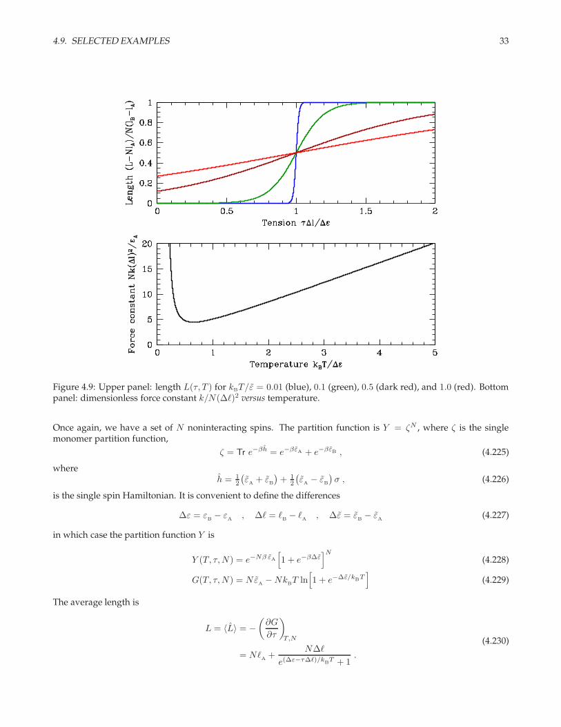
4.9. SELECTED EXAMPLES 33
Figure 4.9: Upper panel: length L(τ, T ) for kBT/ε = 0.01 (blue), 0.1 (green), 0.5 (dark red), and 1.0 (red). Bottompanel: dimensionless force constant k/N(∆ℓ)2 versus temperature.
Once again, we have a set of N noninteracting spins. The partition function is Y = ζN , where ζ is the singlemonomer partition function,
ζ = Tr e−βh = e−βεA + e−βεB , (4.225)
whereh = 1
2
(εA
+ εB
)+ 1
2
(εA− ε
B
)σ , (4.226)
is the single spin Hamiltonian. It is convenient to define the differences
∆ε = εB− ε
A, ∆ℓ = ℓ
B− ℓ
A, ∆ε = ε
B− ε
A(4.227)
in which case the partition function Y is
Y (T, τ,N) = e−Nβ εA
[1 + e−β∆ε
]N(4.228)
G(T, τ,N) = NεA−Nk
BT ln
[1 + e−∆ε/kBT
](4.229)
The average length is
L = 〈L〉 = −(∂G
∂τ
)
T,N
= NℓA
+N∆ℓ
e(∆ε−τ∆ℓ)/kB
T + 1.
(4.230)
34 CHAPTER 4. STATISTICAL ENSEMBLES
The polymer behaves as a spring, and for small τ the spring constant is
k =∂τ
∂L
∣∣∣∣τ=0
=4k
BT
N(∆ℓ)2cosh2
(∆ε
2kBT
). (4.231)
The results are shown in fig. 4.9. Note that length increases with temperature for τ < τ∗ and decreases withtemperature for τ > τ∗. Note also that k diverges at both low and high temperatures. At low T , the energy gap∆ε dominates and L = Nℓ
A, while at high temperatures k
BT dominates and L = 1
2N(ℓA
+ ℓB).
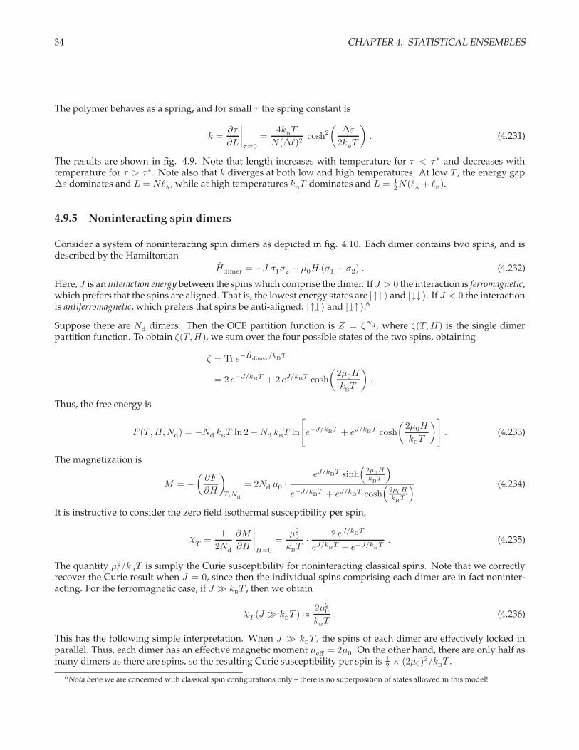
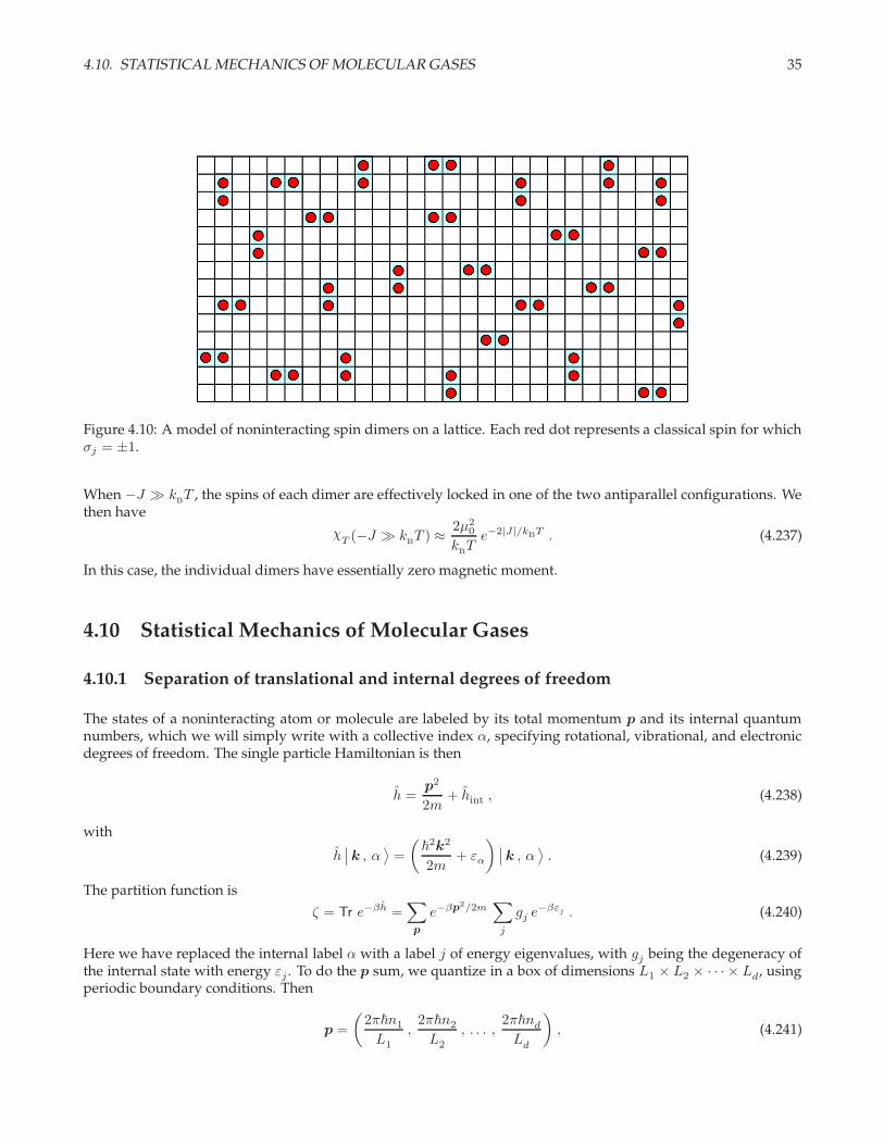
4.9.5 Noninteracting spin dimers
Consider a system of noninteracting spin dimers as depicted in fig. 4.10. Each dimer contains two spins, and isdescribed by the Hamiltonian
Hdimer = −J σ1σ2 − µ0H (σ1 + σ2) . (4.232)
Here, J is an interaction energy between the spins which comprise the dimer. If J > 0 the interaction is ferromagnetic,which prefers that the spins are aligned. That is, the lowest energy states are |↑↑ 〉 and |↓↓ 〉. If J < 0 the interactionis antiferromagnetic, which prefers that spins be anti-aligned: |↑↓ 〉 and |↓↑ 〉.6
Suppose there are Nd dimers. Then the OCE partition function is Z = ζNd , where ζ(T,H) is the single dimerpartition function. To obtain ζ(T,H), we sum over the four possible states of the two spins, obtaining
ζ = Tr e−Hdimer/kBT
= 2 e−J/kBT + 2 eJ/kBT cosh
(2µ0H
kBT
).
Thus, the free energy is
F (T,H,Nd) = −Nd kBT ln 2 −Nd kB
T ln
[e−J/kBT + eJ/kBT cosh
(2µ0H
kBT
)]. (4.233)
The magnetization is
M = −(∂F
∂H
)
T,Nd
= 2Nd µ0 ·eJ/kBT sinh
(2µ0HkB
T
)
e−J/kB
T + eJ/kB
T cosh(
2µ0HkB
T
) (4.234)
It is instructive to consider the zero field isothermal susceptibility per spin,
χT =
1
2Nd
∂M
∂H
∣∣∣∣H=0
=µ2
0
kBT
· 2 eJ/kBT
eJ/kB
T + e−J/kB
T. (4.235)
The quantity µ20/kB
T is simply the Curie susceptibility for noninteracting classical spins. Note that we correctlyrecover the Curie result when J = 0, since then the individual spins comprising each dimer are in fact noninter-acting. For the ferromagnetic case, if J ≫ k
BT , then we obtain
χT (J ≫ k
BT ) ≈ 2µ2
0
kBT. (4.236)
This has the following simple interpretation. When J ≫ kBT , the spins of each dimer are effectively locked in
parallel. Thus, each dimer has an effective magnetic moment µeff = 2µ0. On the other hand, there are only half asmany dimers as there are spins, so the resulting Curie susceptibility per spin is 1
2 × (2µ0)2/k
BT .
6Nota bene we are concerned with classical spin configurations only – there is no superposition of states allowed in this model!
4.10. STATISTICAL MECHANICS OF MOLECULAR GASES 35
Figure 4.10: A model of noninteracting spin dimers on a lattice. Each red dot represents a classical spin for whichσj = ±1.
When −J ≫ kBT , the spins of each dimer are effectively locked in one of the two antiparallel configurations. We
then have
χT (−J ≫ k
BT ) ≈ 2µ2
0
kBTe−2|J|/kBT . (4.237)
In this case, the individual dimers have essentially zero magnetic moment.
4.10 Statistical Mechanics of Molecular Gases
4.10.1 Separation of translational and internal degrees of freedom
The states of a noninteracting atom or molecule are labeled by its total momentum p and its internal quantumnumbers, which we will simply write with a collective index α, specifying rotational, vibrational, and electronicdegrees of freedom. The single particle Hamiltonian is then
h =p2
2m+ hint , (4.238)
with
h∣∣k , α
⟩=
(~
2k2
2m+ εα
) ∣∣k , α⟩. (4.239)
The partition function is
ζ = Tr e−βh =∑
p
e−βp2/2m∑
j
gj e−βεj . (4.240)
Here we have replaced the internal label α with a label j of energy eigenvalues, with gj being the degeneracy ofthe internal state with energy εj . To do the p sum, we quantize in a box of dimensions L1 × L2 × · · · × Ld, usingperiodic boundary conditions. Then
p =
(2π~n1
L1
,2π~n2
L2
, . . . ,2π~nd
Ld
), (4.241)
36 CHAPTER 4. STATISTICAL ENSEMBLES
where each ni is an integer. Since the differences between neighboring quantized p vectors are very tiny, we canreplace the sum over p by an integral:
∑
p
−→∫
ddp
∆p1 · · ·∆pd
(4.242)
where the volume in momentum space of an elementary rectangle is
∆p1 · · ·∆pd =(2π~)d
L1 · · ·Ld
=(2π~)d
V. (4.243)
Thus,
ζ = V
∫ddp
(2π~)de−p2/2mkBT
∑
j
gj e−εj/kBT = V λ−d
T ξ (4.244)
ξ(T ) =∑
j
gj e−εj/kBT . (4.245)
Here, ξ(T ) is the internal coordinate partition function. The full N -particle ordinary canonical partition function isthen
ZN =1
N !
(V
λdT
)N
ξN (T ) . (4.246)
Using Stirling’s approximation, we find the Helmholtz free energy F = −kBT lnZ is
F (T, V,N) = −NkBT
[ln
(V
NλdT
)+ 1 + ln ξ(T )
]
= −NkBT
[ln
(V
NλdT
)+ 1
]+Nϕ(T ) ,
(4.247)
where
ϕ(T ) = −kBT ln ξ(T ) (4.248)
is the internal coordinate contribution to the single particle free energy. We could also compute the partitionfunction in the Gibbs (T, p,N) ensemble:
Y (T, p,N) = e−βG(T,p,N) =1
V0
∞∫
0
dV e−βpV Z(T, V,N)
=
(k
BT
pV0
)(k
BT
p λdT
)NξN (T ) .
(4.249)
Thus, in the thermodynamic limit,
µ(T, p) =G(T, p,N)
N= k
BT ln
(p λd
T
kBT
)− k
BT ln ξ(T )
= kBT ln
(p λd
T
kBT
)+ ϕ(T ) .
(4.250)
4.10. STATISTICAL MECHANICS OF MOLECULAR GASES 37
4.10.2 Ideal gas law
Since the internal coordinate contribution to the free energy is volume-independent, we have
V =
(∂G
∂p
)
T,N
=Nk
BT
p, (4.251)
and the ideal gas law applies. The entropy is
S = −(∂G
∂T
)
p,N
= NkB
[ln
(k
BT
pλdT
)+ 1 + 1
2d
]−Nϕ′(T ) , (4.252)
and therefore the heat capacity is
Cp = T
(∂S
∂T
)
p,N
=(
12d+ 1
)Nk
B−NT ϕ′′(T ) (4.253)
CV = T
(∂S
∂T
)
V,N
= 12dNkB
−NT ϕ′′(T ) . (4.254)
Thus, any temperature variation in Cp must be due to the internal degrees of freedom.
4.10.3 The internal coordinate partition function
At energy scales of interest we can separate the internal degrees of freedom into distinct classes, writing
hint = hrot + hvib + helec (4.255)
as a sum over internal Hamiltonians governing rotational, vibrational, and electronic degrees of freedom. Then
ξint = ξrot · ξvib · ξelec . (4.256)
Associated with each class of excitation is a characteristic temperatureΘ. Rotational and vibrational temperaturesof a few common molecules are listed in table tab. 4.1.
4.10.4 Rotations
Consider a class of molecules which can be approximated as an axisymmetric top. The rotational Hamiltonian isthen
hrot =L
2a + L
2b
2I1+
L2c
2I3
=~
2L(L+ 1)
2I1+
(1
2I3− 1
2I1
)L
2c ,
(4.257)
where na.b,c(t) are the principal axes, with nc the symmetry axis, and La,b,c are the components of the angularmomentum vector L about these instantaneous body-fixed principal axes. The components of L along space-fixedaxes x, y, z are written as Lx,y,z. Note that
[Lµ , Lc
]= nν
c
[Lµ , Lν
]+[Lµ , nν
c
]Lν = iǫµνλ n
νc L
λ + iǫµνλ nλc L
ν = 0 , (4.258)
38 CHAPTER 4. STATISTICAL ENSEMBLES
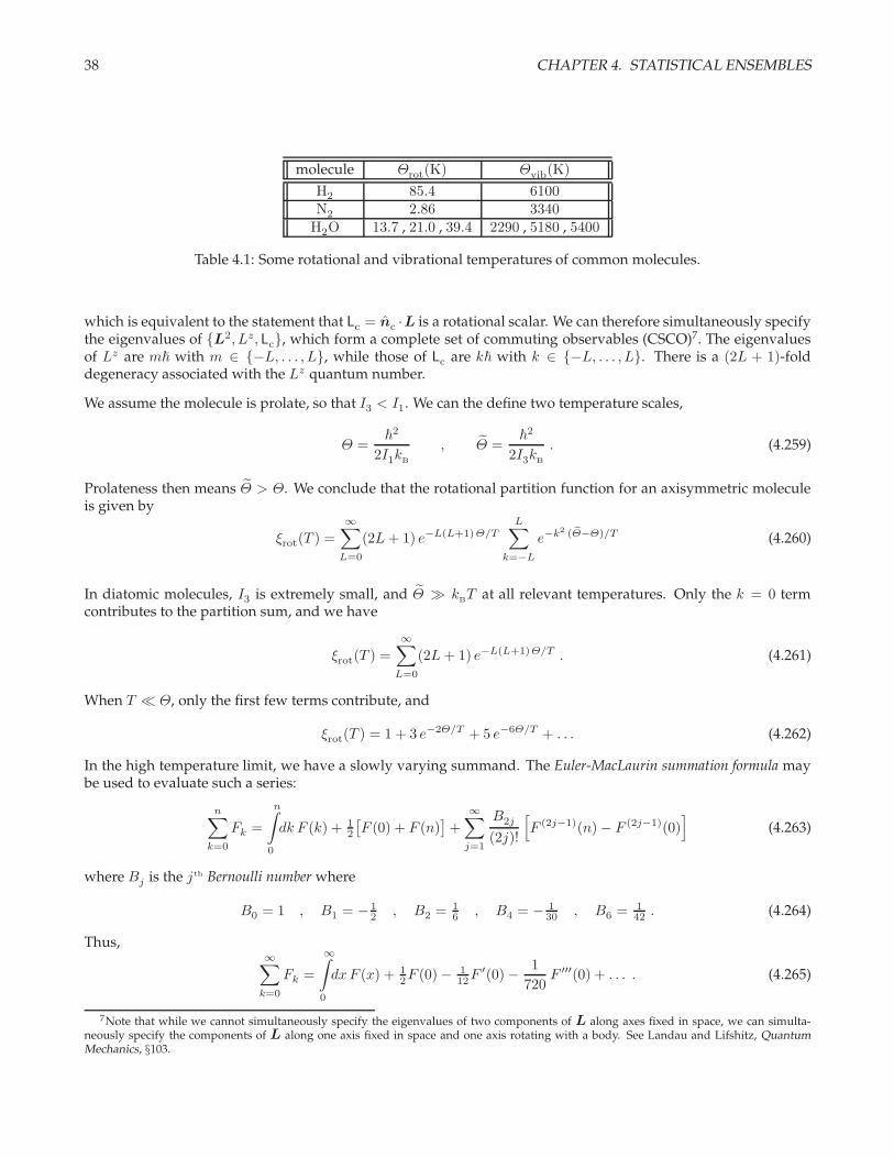
molecule Θrot(K) Θvib(K)
H2 85.4 6100N2 2.86 3340
H2O 13.7 , 21.0 , 39.4 2290 , 5180 , 5400
Table 4.1: Some rotational and vibrational temperatures of common molecules.
which is equivalent to the statement that Lc = nc ·L is a rotational scalar. We can therefore simultaneously specifythe eigenvalues of L2, Lz, Lc, which form a complete set of commuting observables (CSCO)7. The eigenvaluesof Lz are m~ with m ∈ −L, . . . , L, while those of Lc are k~ with k ∈ −L, . . . , L. There is a (2L + 1)-folddegeneracy associated with the Lz quantum number.
We assume the molecule is prolate, so that I3 < I1. We can the define two temperature scales,
Θ =~
2
2I1kB
, Θ =~
2
2I3kB
. (4.259)
Prolateness then means Θ > Θ. We conclude that the rotational partition function for an axisymmetric moleculeis given by
ξrot(T ) =
∞∑
L=0
(2L+ 1) e−L(L+1)Θ/TL∑
k=−L
e−k2 ( eΘ−Θ)/T (4.260)
In diatomic molecules, I3 is extremely small, and Θ ≫ kBT at all relevant temperatures. Only the k = 0 term
contributes to the partition sum, and we have
ξrot(T ) =
∞∑
L=0
(2L+ 1) e−L(L+1)Θ/T . (4.261)
When T ≪ Θ, only the first few terms contribute, and
ξrot(T ) = 1 + 3 e−2Θ/T + 5 e−6Θ/T + . . . (4.262)
In the high temperature limit, we have a slowly varying summand. The Euler-MacLaurin summation formula maybe used to evaluate such a series:
n∑
k=0
Fk =
n∫
0
dk F (k) + 12
[F (0) + F (n)
]+
∞∑
j=1
B2j
(2j)!
[F (2j−1)(n) − F (2j−1)(0)
](4.263)
where Bj is the jth Bernoulli number where
B0 = 1 , B1 = − 12 , B2 = 1
6 , B4 = − 130 , B6 = 1
42 . (4.264)
Thus,∞∑
k=0
Fk =
∞∫
0
dxF (x) + 12F (0) − 1
12F′(0) − 1
720F ′′′(0) + . . . . (4.265)
7Note that while we cannot simultaneously specify the eigenvalues of two components of L along axes fixed in space, we can simulta-neously specify the components of L along one axis fixed in space and one axis rotating with a body. See Landau and Lifshitz, QuantumMechanics, §103.
4.10. STATISTICAL MECHANICS OF MOLECULAR GASES 39
We have F (x) = (2x+ 1) e−x(x+1)Θ/T , for which∞∫0
dxF (x) = TΘ , hence
ξrot =T
Θ+
1
3+
1
15
Θ
T+
4
315
(Θ
T
)2+ . . . . (4.266)
Recall thatϕ(T ) = −kBT ln ξ(T ). We conclude thatϕrot(T ) ≈ −3k
BT e−2Θ/T for T ≪ Θ andϕrot(T ) ≈ −k
BT ln(T/Θ)
for T ≫ Θ. We have seen that the internal coordinate contribution to the heat capacity is ∆CV = −NTϕ′′(T ). Fordiatomic molecules, then, this contribution is exponentially suppressed for T ≪ Θ, while for high temperatureswe have ∆CV = Nk
B. One says that the rotational excitations are ‘frozen out’ at temperatures much below Θ.
Including the first few terms, we have
∆CV (T ≪ Θ) = 12NkB
(Θ
T
)2
e−2Θ/T + . . . (4.267)
∆CV (T ≫ Θ) = NkB
1 +
1
45
(Θ
T
)2+
16
945
(Θ
T
)3+ . . .
. (4.268)
Note that CV overshoots its limiting value of NkB
and asymptotically approaches it from above.
Special care must be taken in the case of homonuclear diatomic molecules, for then only even or odd L states areallowed, depending on the total nuclear spin. This is discussed below in §4.10.7.
For polyatomic molecules, the moments of inertia generally are large enough that the molecule’s rotations can beconsidered classically. We then have
ε(La, Lb, Lc) =L
2a
2I1+
L2b
2I2+
L2c
2I3. (4.269)
We then have
ξrot(T ) =1
grot
∫dLa dLb dLc dφ dθ dψ
(2π~)3e−ε(La Lb Lc)/kBT , (4.270)
where (φ, θ ψ) are the Euler angles. Recall φ ∈ [0, 2π], θ ∈ [0, π], and ψ ∈ [0, 2π]. The factor grot accounts forphysically indistinguishable orientations of the molecule brought about by rotations, which can happen whenmore than one of the nuclei is the same. We then have
ξrot(T ) =
(2k
BT
~2
)3/2√πI1I2I3 . (4.271)
This leads to ∆CV = 32NkB
.
4.10.5 Vibrations
Vibrational frequencies are often given in units of inverse wavelength, such as cm−1, called a wavenumber. Toconvert to a temperature scale T ∗, we write k
BT ∗ = hν = hc/λ, hence T ∗ = (hc/k
B)λ−1, and we multiply by
hc
kB
= 1.436 K · cm . (4.272)
For example, infrared absorption (∼ 50 cm−1 to 104 cm−1) reveals that the ‘asymmetric stretch’ mode of the H2Omolecule has a vibrational frequency of ν = 3756 cm−1. The corresponding temperature scale is T ∗ = 5394 K.
40 CHAPTER 4. STATISTICAL ENSEMBLES
Vibrations are normal modes of oscillations. A single normal mode Hamiltonian is of the form
h =p2
2m+ 1
2mω2q2 = ~ω
(a†a+ 1
2
). (4.273)
In general there are many vibrational modes, hence many normal mode frequencies ωα. We then must sum overall of them, resulting in
ξvib =∏
α
ξ(α)vib . (4.274)
For each such normal mode, the contribution is
ξ =
∞∑
n=0
e−(n+ 12)~ω/kBT = e−~ω/2kBT
∞∑
n=0
(e−~ω/kBT
)n
=e−~ω/2kBT
1 − e−~ω/kB
T=
1
2 sinh(Θ/2T ),
(4.275)
where Θ = ~ω/kB
. Then
ϕ = kBT ln
(2 sinh(Θ/2T )
)
= 12kB
Θ + kBT ln
(1 − e−Θ/T
).
(4.276)
The contribution to the heat capacity is
∆CV = NkB
(Θ
T
)2eΘ/T
(eΘ/T − 1)2
=
Nk
B(Θ/T )2 exp(−Θ/T ) (T → 0)
NkB
(T → ∞)
(4.277)
4.10.6 Two-level systems : Schottky anomaly
Consider now a two-level system, with energies ε0 and ε1. We define ∆ ≡ ε1 − ε0 and assume without loss ofgenerality that ∆ > 0. The partition function is
ζ = e−βε0 + e−βε1 = e−βε0
(1 + e−β∆
). (4.278)
The free energy is
f = −kBT ln ζ = ε0 − k
BT ln
(1 + e−∆/kBT
). (4.279)
The entropy for a given two level system is then
s = − ∂f
∂T= k
Bln(1 + e−∆/kBT
)+
∆
T· 1
e∆/kB
T + 1(4.280)
and the heat capacity is = T (∂s/∂T ), i.e.
c(T ) =∆2
kBT 2
· e∆/kBT
(e∆/k
BT + 1
)2 . (4.281)
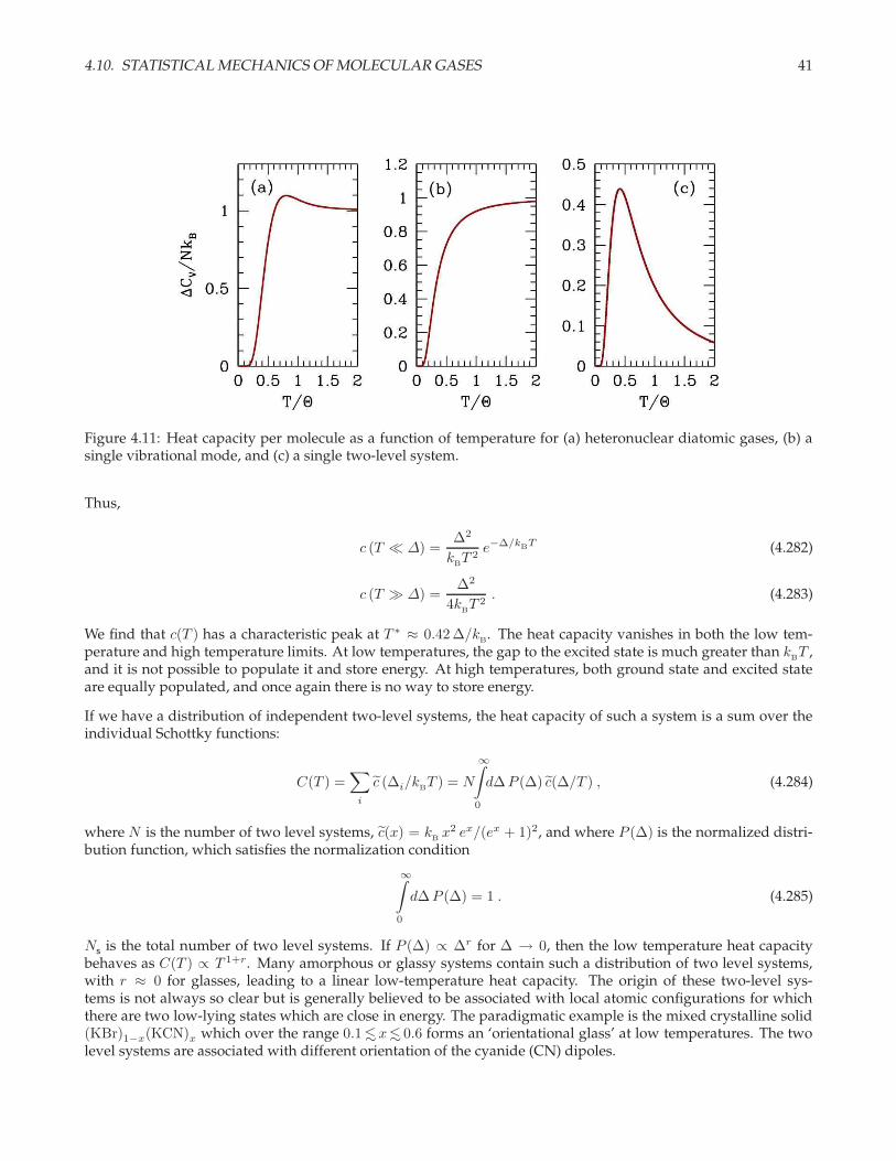
4.10. STATISTICAL MECHANICS OF MOLECULAR GASES 41
Figure 4.11: Heat capacity per molecule as a function of temperature for (a) heteronuclear diatomic gases, (b) asingle vibrational mode, and (c) a single two-level system.
Thus,
c (T ≪ ∆) =∆2
kBT 2
e−∆/kBT (4.282)
c (T ≫ ∆) =∆2
4kBT 2
. (4.283)
We find that c(T ) has a characteristic peak at T ∗ ≈ 0.42 ∆/kB
. The heat capacity vanishes in both the low tem-perature and high temperature limits. At low temperatures, the gap to the excited state is much greater than k
BT ,
and it is not possible to populate it and store energy. At high temperatures, both ground state and excited stateare equally populated, and once again there is no way to store energy.
If we have a distribution of independent two-level systems, the heat capacity of such a system is a sum over theindividual Schottky functions:
C(T ) =∑
i
c (∆i/kBT ) = N
∞∫
0
d∆P (∆) c(∆/T ) , (4.284)
where N is the number of two level systems, c(x) = kBx2 ex/(ex + 1)2, and where P (∆) is the normalized distri-
bution function, which satisfies the normalization condition
∞∫
0
d∆P (∆) = 1 . (4.285)
Ns
is the total number of two level systems. If P (∆) ∝ ∆r for ∆ → 0, then the low temperature heat capacitybehaves as C(T ) ∝ T 1+r. Many amorphous or glassy systems contain such a distribution of two level systems,with r ≈ 0 for glasses, leading to a linear low-temperature heat capacity. The origin of these two-level sys-tems is not always so clear but is generally believed to be associated with local atomic configurations for whichthere are two low-lying states which are close in energy. The paradigmatic example is the mixed crystalline solid(KBr)1−x(KCN)x which over the range 0.1<∼x<∼ 0.6 forms an ‘orientational glass’ at low temperatures. The twolevel systems are associated with different orientation of the cyanide (CN) dipoles.

42 CHAPTER 4. STATISTICAL ENSEMBLES
4.10.7 Electronic and nuclear excitations
For a monatomic gas, the internal coordinate partition function arises due to electronic and nuclear degrees offreedom. Let’s first consider the electronic degrees of freedom. We assume that k
BT is small compared with
energy differences between successive electronic shells. The atomic ground state is then computed by filling upthe hydrogenic orbitals until all the electrons are used up. If the atomic number is a ‘magic number’ (A = 2 (He),10 (Ne), 18 (Ar), 36 (Kr), 54 (Xe), etc.) then the atom has all shells filled and L = 0 and S = 0. Otherwise the lastshell is partially filled and one or both of L and S will be nonzero. The atomic ground state configuration 2J+1LS
is then determined by Hund’s rules:
1. The LS multiplet with the largest S has the lowest energy.
2. If the largest value of S is associated with several multiplets, the multiplet with the largest L has the lowestenergy.
3. If an incomplete shell is not more than half-filled, then the lowest energy state has J = |L− S|. If the shell ismore than half-filled, then J = L+ S.
The last of Hund’s rules distinguishes between the (2S + 1)(2L + 1) states which result upon fixing S and L asper rules #1 and #2. It arises due to the atomic spin-orbit coupling, whose effective Hamiltonian may be written
H = ΛL · S, where Λ is the Russell-Saunders coupling. If the last shell is less than or equal to half-filled, thenΛ > 0 and the ground state has J = |L − S|. If the last shell is more than half-filled, the coupling is inverted, i.e.Λ < 0, and the ground state has J = L+ S.8
The electronic contribution to ξ is then
ξelec =
L+S∑
J=|L−S|
(2J + 1) e−∆ε(L,S,J)/kBT (4.286)
where∆ε(L, S, J) = 1
2Λ[J(J + 1) − L(L+ 1) − S(S + 1)
]. (4.287)
At high temperatures, kBT is larger than the energy difference between the different J multiplets, and we have
ξelec ∼ (2L + 1)(2S + 1) e−βε0 , where ε0 is the ground state energy. At low temperatures, a particular value ofJ is selected – that determined by Hund’s third rule – and we have ξelec ∼ (2J + 1) e−βε0 . If, in addition, thereis a nonzero nuclear spin I , then we also must include a factor ξnuc = (2I + 1), neglecting the small hyperfinesplittings due to the coupling of nuclear and electronic angular momenta.
For heteronuclear diatomic molecules, i.e. molecules composed from two different atomic nuclei, the internal par-
tition function simply receives a factor of ξelec · ξ(1)nuc · ξ(2)nuc, where the first term is a sum over molecular electronic
states, and the second two terms arise from the spin degeneracies of the two nuclei. For homonuclear diatomicmolecules, the exchange of nuclear centers is a symmetry operation, and does not represent a distinct quantumstate. To correctly count the electronic states, we first assume that the total electronic spin is S = 0. This is gen-erally a very safe assumption. Exchange symmetry now puts restrictions on the possible values of the molecularangular momentum L, depending on the total nuclear angular momentum Itot. If Itot is even, then the molecularangular momentum L must also be even. If the total nuclear angular momentum is odd, then Lmust be odd. Thisis so because the molecular ground state configuration is 1Σ+
g .9
The total number of nuclear states for the molecule is (2I + 1)2, of which some are even under nuclear exchange,and some are odd. The number of even states, corresponding to even total nuclear angular momentum is written
8See e.g. §72 of Landau and Lifshitz, Quantum Mechanics, which, in my humble estimation, is the greatest physics book ever written.9See Landau and Lifshitz, Quantum Mechanics, §86.
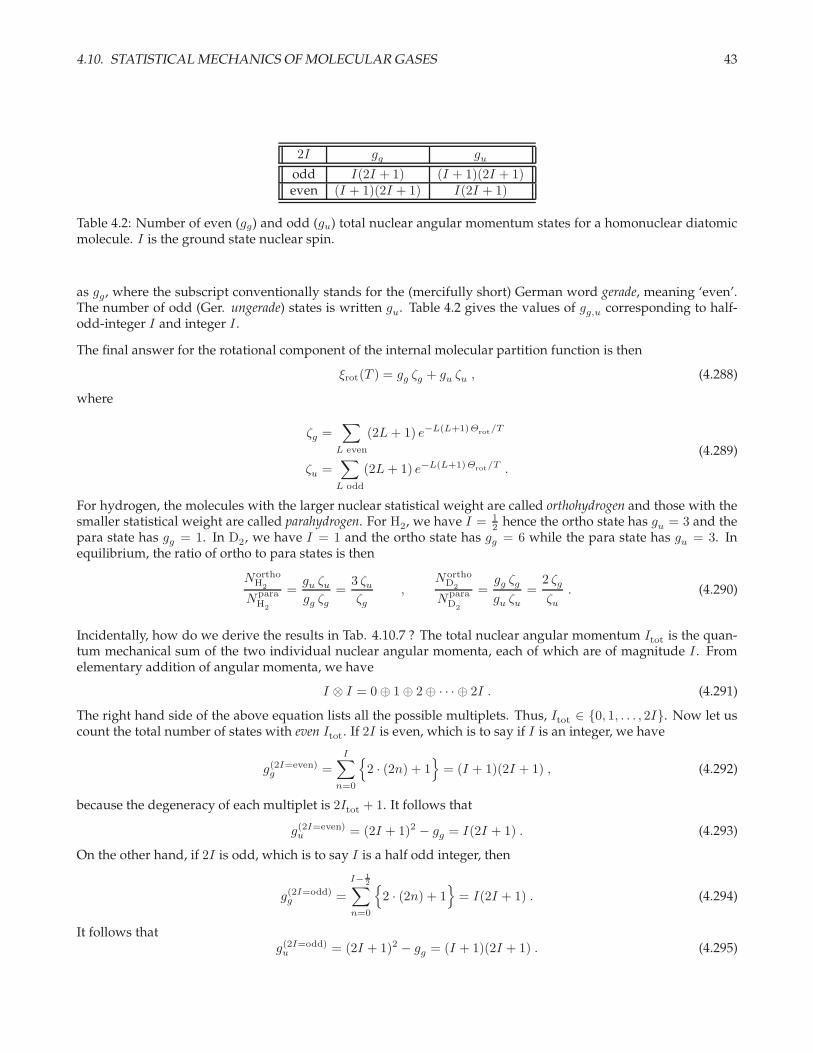
4.10. STATISTICAL MECHANICS OF MOLECULAR GASES 43
2I gg gu
odd I(2I + 1) (I + 1)(2I + 1)even (I + 1)(2I + 1) I(2I + 1)
Table 4.2: Number of even (gg) and odd (gu) total nuclear angular momentum states for a homonuclear diatomicmolecule. I is the ground state nuclear spin.
as gg, where the subscript conventionally stands for the (mercifully short) German word gerade, meaning ‘even’.The number of odd (Ger. ungerade) states is written gu. Table 4.2 gives the values of gg,u corresponding to half-odd-integer I and integer I .
The final answer for the rotational component of the internal molecular partition function is then
ξrot(T ) = gg ζg + gu ζu , (4.288)
where
ζg =∑
L even
(2L+ 1) e−L(L+1)Θrot/T
ζu =∑
L odd
(2L+ 1) e−L(L+1)Θrot/T .
(4.289)
For hydrogen, the molecules with the larger nuclear statistical weight are called orthohydrogen and those with thesmaller statistical weight are called parahydrogen. For H2, we have I = 1
2 hence the ortho state has gu = 3 and thepara state has gg = 1. In D2, we have I = 1 and the ortho state has gg = 6 while the para state has gu = 3. Inequilibrium, the ratio of ortho to para states is then
NorthoH2
NparaH2
=gu ζugg ζg
=3 ζuζg
,Northo
D2
NparaD2
=gg ζggu ζu
=2 ζgζu
. (4.290)
Incidentally, how do we derive the results in Tab. 4.10.7 ? The total nuclear angular momentum Itot is the quan-tum mechanical sum of the two individual nuclear angular momenta, each of which are of magnitude I . Fromelementary addition of angular momenta, we have
I ⊗ I = 0 ⊕ 1 ⊕ 2 ⊕ · · · ⊕ 2I . (4.291)
The right hand side of the above equation lists all the possible multiplets. Thus, Itot ∈ 0, 1, . . . , 2I. Now let uscount the total number of states with even Itot. If 2I is even, which is to say if I is an integer, we have
g(2I=even)g =
I∑
n=0
2 · (2n) + 1
= (I + 1)(2I + 1) , (4.292)
because the degeneracy of each multiplet is 2Itot + 1. It follows that
g(2I=even)u = (2I + 1)2 − gg = I(2I + 1) . (4.293)
On the other hand, if 2I is odd, which is to say I is a half odd integer, then
g(2I=odd)g =
I− 12∑
n=0
2 · (2n) + 1
= I(2I + 1) . (4.294)
It follows thatg(2I=odd)
u = (2I + 1)2 − gg = (I + 1)(2I + 1) . (4.295)
44 CHAPTER 4. STATISTICAL ENSEMBLES
4.11 Appendix I : Additional Examples
4.11.1 Three state system
Consider a spin-1 particle where σ = −1, 0,+1. We model this with the single particle Hamiltonian
h = −µ0H σ + ∆(1 − σ2) . (4.296)
We can also interpret this as describing a spin if σ = ±1 and a vacancy if σ = 0. The parameter ∆ then representsthe vacancy formation energy. The single particle partition function is
ζ = Tr e−βh = e−β∆ + 2 cosh(βµ0H) . (4.297)
With Ns
distinguishable noninteracting spins (e.g. at different sites in a crystalline lattice), we have Z = ζNs and
F ≡ Nsf = −k
BT lnZ = −N
sk
BT ln
[e−β∆ + 2 cosh(βµ0H)
], (4.298)
where f = −kBT ln ζ is the free energy of a single particle. Note that
nV
= 1 − σ2 =∂h
∂∆(4.299)
m = µ0 σ = − ∂h
∂H(4.300)
are the vacancy number and magnetization, respectively. Thus,
nV
=⟨n
V
⟩=∂f
∂∆=
e−∆/kBT
e−∆/kB
T + 2 cosh(µ0H/kBT )
(4.301)
and
m =⟨m⟩
= − ∂f
∂H=
2µ0 sinh(µ0H/kBT )
e−∆/kB
T + 2 cosh(µ0H/kBT )
. (4.302)
At weak fields we can compute
χT =
∂m
∂H
∣∣∣∣H=0
=µ2
0
kBT
· 2
2 + e−∆/kB
T. (4.303)
We thus obtain a modified Curie law. At temperatures T ≪ ∆/kB
, the vacancies are frozen out and we recover theusual Curie behavior. At high temperatures, where T ≫ ∆/k
B, the low temperature result is reduced by a factor
of 23 , which accounts for the fact that one third of the time the particle is in a nonmagnetic state with σ = 0.
4.11.2 Spins and vacancies on a surface
PROBLEM: A collection of spin- 12 particles is confined to a surface with N sites. For each site, let σ = 0 if there
is a vacancy, σ = +1 if there is particle present with spin up, and σ = −1 if there is a particle present with spindown. The particles are non-interacting, and the energy for each site is given by ε = −Wσ2, where −W < 0 is thebinding energy.
(a) Let Q = N↑ +N↓ be the number of spins, and N0 be the number of vacancies. The surface magnetization is
M = N↑ −N↓. Compute, in the microcanonical ensemble, the statistical entropy S(Q,M).
4.11. APPENDIX I : ADDITIONAL EXAMPLES 45
(b) Let q = Q/N and m = M/N be the dimensionless particle density and magnetization density, respectively.Assuming that we are in the thermodynamic limit, where N , Q, and M all tend to infinity, but with q and mfinite, Find the temperature T (q,m). Recall Stirling’s formula
ln(N !) = N lnN −N + O(lnN) .
(c) Show explicitly that T can be negative for this system. What does negative T mean? What physical degreesof freedom have been left out that would avoid this strange property?
SOLUTION: There is a constraint on N↑, N0, and N↓:
N↑ +N0 +N↓ = Q+N0 = N . (4.304)
The total energy of the system is E = −WQ.
(a) The number of states available to the system is
Ω =N !
N↑!N0!N↓!. (4.305)
Fixing Q and M , along with the above constraint, is enough to completely determine N↑, N0, N↓:
N↑ = 12 (Q+M) , N0 = N −Q , N↓ = 1
2 (Q−M) , (4.306)
whence
Ω(Q,M) =N ![
12 (Q+M)
]![
12 (Q−M)
]! (N −Q)!
. (4.307)
The statistical entropy is S = kB
ln Ω:
S(Q,M) = kB
ln(N !) − kB
ln[
12 (Q+M)!
]− k
Bln[
12 (Q−M)!
]− k
Bln[(N −Q)!
]. (4.308)
(b) Now we invoke Stirling’s rule,ln(N !) = N lnN −N + O(lnN) , (4.309)
to obtain
ln Ω(Q,M) = N lnN −N − 12 (Q+M) ln
[12 (Q+M)
]+ 1
2 (Q+M)
− 12 (Q−M) ln
[12 (Q−M)
]+ 1
2 (Q−M)
− (N −Q) ln(N −Q) + (N −Q)
= N lnN − 12Q ln
[14 (Q2 −M2)
]− 1
2M ln
(Q+M
Q−M
)
(4.310)
Combining terms,
ln Ω(Q,M) = −Nq ln[
12
√q2 −m2
]− 1
2Nm ln
(q +m
q −m
)−N(1 − q) ln(1 − q) , (4.311)
where Q = Nq and M = Nm. Note that the entropy S = kB
ln Ω is extensive. The statistical entropy per siteis thus
s(q,m) = −kBq ln
[12
√q2 −m2
]− 1
2kBm ln
(q +m
q −m
)− k
B(1 − q) ln(1 − q) . (4.312)
46 CHAPTER 4. STATISTICAL ENSEMBLES
The temperature is obtained from the relation
1
T=
(∂S
∂E
)
M
=1
W
(∂s
∂q
)
m
=1
Wln(1 − q) − 1
Wln[
12
√q2 −m2
].
(4.313)
Thus,
T =W/k
B
ln[2(1 − q)/
√q2 −m2
] . (4.314)
(c) We have 0 ≤ q ≤ 1 and −q ≤ m ≤ q, so T is real (thank heavens!). But it is easy to choose q,m such thatT < 0. For example, when m = 0 we have T = W/k
Bln(2q−1−2) and T < 0 for all q ∈
(23 , 1]. The reason for
this strange state of affairs is that the entropy S is bounded, and is not an monotonically increasing function
of the energyE (or the dimensionless quantity Q). The entropy is maximized for N ↑= N0 = N↓ = 13 , which
says m = 0 and q = 23 . Increasing q beyond this point (with m = 0 fixed) starts to reduce the entropy, and
hence (∂S/∂E) < 0 in this range, which immediately gives T < 0. What we’ve left out are kinetic degrees offreedom, such as vibrations and rotations, whose energies are unbounded, and which result in an increasingS(E) function.
4.11.3 Fluctuating interface
Consider an interface between two dissimilar fluids. In equilibrium, in a uniform gravitational field, the denserfluid is on the bottom. Let z = z(x, y) be the height the interface between the fluids, relative to equilibrium. Thepotential energy is a sum of gravitational and surface tension terms, with
Ugrav =
∫d2x
z∫
0
dz′ ∆ρ g z′ (4.315)
Usurf =
∫d2x 1
2σ (∇z)2 . (4.316)
We won’t need the kinetic energy in our calculations, but we can include it just for completeness. It isn’t so clearhow to model it a priori so we will assume a rather general form
T =
∫d2x
∫d2x′ 1
2µ(x,x′)∂z(x, t)
∂t
∂z(x′, t)
∂t. (4.317)
We assume that the (x, y) plane is a rectangle of dimensions Lx × Ly . We also assume µ(x,x′) = µ(|x − x′|
). We
can then Fourier transformz(x) =
(Lx Ly
)−1/2∑
k
zk eik·x , (4.318)
where the wavevectors k are quantized according to
k =2πnx
Lx
x +2πny
Ly
y , (4.319)
with integer nx and ny , if we impose periodic boundary conditions (for calculational convenience). The La-grangian is then
L =1
2
∑
k
[µk
∣∣zk∣∣2 −
(g∆ρ+ σk2
) ∣∣zk∣∣2], (4.320)
4.11. APPENDIX I : ADDITIONAL EXAMPLES 47
where
µk =
∫d2xµ
(|x|)e−ik·x . (4.321)
Since z(x, t) is real, we have the relation z−k = z∗k, therefore the Fourier coefficients at k and −k are not indepen-dent. The canonical momenta are given by
pk =∂L
∂z∗k= µk zk , p∗k =
∂L
∂zk= µk z
∗k (4.322)
The Hamiltonian is then
H =∑
k
′[pk z
∗k + p∗k zk
]− L (4.323)
=∑
k
′[ |pk|2µ
k
+(g∆ρ+ σk2
)|zk|2
], (4.324)
where the prime on the k sum indicates that only one of the pair k,−k is to be included, for each k.
We may now compute the ordinary canonical partition function:
Z =∏
k
′∫d2pk d
2zk(2π~)2
e−|pk|2/µkkBT e−(g ∆ρ+σk2) |zk|
2/kBT
=∏
k
′(k
BT
2~
)2( µk
g∆ρ+ σk2
).
(4.325)
Thus,
F = −kBT∑
k
ln
(k
BT
2~Ωk
), (4.326)
where10
Ωk =
(g∆ρ+ σk2
µk
)1/2
. (4.327)
is the normal mode frequency for surface oscillations at wavevector k. For deep water waves, it is appropriate totake µk = ∆ρ
/|k|, where ∆ρ = ρ
L− ρ
G≈ ρ
Lis the difference between the densities of water and air.
It is now easy to compute the thermal average
⟨|zk|2
⟩=
∫d2zk |zk|2 e−(g ∆ρ+σk2) |zk|
2/kBT
/∫d2zk e
−(g ∆ρ+σk2) |zk|2/kBT
=k
BT
g∆ρ+ σk2.
(4.328)
Note that this result does not depend on µk, i.e. on our choice of kinetic energy. One defines the correlation function
C(x) ≡⟨z(x) z(0)
⟩=
1
LxLy
∑
k
⟨|zk|2
⟩eik·x =
∫d2k
(2π)2
(k
BT
g∆ρ+ σk2
)eik·x
=k
BT
4πσ
∞∫
0
dqeik|x|
√q2 + ξ2
=k
BT
4πσK0
(|x|/ξ
),
(4.329)
10Note that there is no prime on the k sum for F , as we have divided the logarithm of Z by two and replaced the half sum by the wholesum.
48 CHAPTER 4. STATISTICAL ENSEMBLES
where ξ =√g∆ρ/σ is the correlation length, and where K0(z) is the Bessel function of imaginary argument. The
asymptotic behavior ofK0(z) for small z isK0(z) ∼ ln(2/z), whereas for large z one hasK0(z) ∼ (π/2z)1/2 e−z . Wesee that on large length scales the correlations decay exponentially, but on small length scales they diverge. Thisdivergence is due to the improper energetics we have assigned to short wavelength fluctuations of the interface.Roughly, it can cured by imposing a cutoff on the integral, or by insisting that the shortest distance scale is amolecular diameter.
4.11.4 Dissociation of molecular hydrogen
Consider the reaction
H −− p+ + e− . (4.330)
In equilibrium, we have
µH = µp + µe . (4.331)
What is the relationship between the temperature T and the fraction x of hydrogen which is dissociated?
Let us assume a fraction x of the hydrogen is dissociated. Then the densities of H, p, and e are then
nH = (1 − x)n , np = xn , ne = xn . (4.332)
The single particle partition function for each species is
ζ =gN
N !
(V
λ3T
)N
e−Nεint/kBT , (4.333)
where g is the degeneracy and εint the internal energy for a given species. We have εint = 0 for p and e, andεint = −∆ for H, where ∆ = e2/2a
B= 13.6 eV, the binding energy of hydrogen. Neglecting hyperfine splittings11,
we have gH = 4, while ge = gp = 2 because each has spin S = 12 . Thus, the associated grand potentials are
ΩH = −gH V kBT λ−3
T,H e(µH+∆)/kBT (4.334)
Ωp = −gp V kBT λ−3
T,p eµp/kBT (4.335)
Ωe = −ge V kBT λ−3
T,e eµe/kBT , (4.336)
where
λT,a =
√2π~2
makBT
(4.337)
for species a. The corresponding number densities are
n =1
V
(∂Ω
∂µ
)
T,V
= g λ−3T e(µ−εint)/kBT , (4.338)
and the fugacity z = eµ/kBT of a given species is given by
z = g−1nλ3T e
εint/kBT . (4.339)
11The hyperfine splitting in hydrogen is on the order of (me/mp) α4 mec2 ∼ 10−6 eV, which is on the order of 0.01 K. Here α = e2/~c is
the fine structure constant.

4.11. APPENDIX I : ADDITIONAL EXAMPLES 49
We now invoke µH = µp + µe, which says zH = zp ze, or
g−1H nH λ
3T,H e
−∆/kBT =(g−1p np λ
3T,p
)(g−1e ne λ
3T,e
), (4.340)
which yields (x2
1 − x
)nλ3
T = e−∆/kBT , (4.341)
where λT =√
2π~2/m∗kBT , with m∗ = mpme/mH ≈ me. Note that
λT = aB
√4πmH
mp
√∆
kBT, (4.342)
where aB
= 0.529 A is the Bohr radius. Thus, we have
(x2
1 − x
)· (4π)3/2 ν =
(T
T0
)3/2
e−T0/T , (4.343)
where T0 = ∆/kB
= 1.578×10⁵ K and ν = na3B
. Consider for example a temperatureT = 3000 K, for which T0/T =52.6, and assume that x = 1
2 . We then find ν = 1.69×10⁻²⁷, corresponding to a density of n = 1.14×10⁻² cm−3. At
this temperature, the fraction of hydrogen molecules in their first excited (2s) state is x′ ∼ e−T0/2T = 3.8 × 10⁻¹².This is quite striking: half the hydrogen atoms are completely dissociated, which requires an energy of ∆, yetthe number in their first excited state, requiring energy 1
2∆, is twelve orders of magnitude smaller. The studentshould reflect on why this can be the case.