Contents

1 Introduction 1

2 Physics of n− n Oscillation 42.1 Beyond the Standard Model : Grand Unification Theory . . . 4

2.1.1 SU(5) . . . . . . . . . . . . . . . . . . . . . . . . . . . 42.1.2 SO(10) . . . . . . . . . . . . . . . . . . . . . . . . . . 6

2.2 Prediction for n−n Oscillation in L-R Symmetric Gauge Theory 72.3 Phenomenology of Neutron Oscillations . . . . . . . . . . . . 8

2.3.1 Free Neutron Oscillations . . . . . . . . . . . . . . . . 92.3.2 Oscillation of Neutrons in an External Field . . . . . . 10

3 Super-Kamiokande 113.1 Cherenkov Radiation . . . . . . . . . . . . . . . . . . . . . . . 113.2 Detector . . . . . . . . . . . . . . . . . . . . . . . . . . . . . . 12

3.2.1 Water Tank . . . . . . . . . . . . . . . . . . . . . . . . 123.2.2 Photomultiplier Tubes . . . . . . . . . . . . . . . . . . 133.2.3 PMT Support Structure and Others . . . . . . . . . . 163.2.4 Water Purification . . . . . . . . . . . . . . . . . . . . 183.2.5 Electronics and Data Acquisition System . . . . . . . 18

3.3 Calibrations . . . . . . . . . . . . . . . . . . . . . . . . . . . . 223.3.1 Water Transparency Measurement . . . . . . . . . . . 223.3.2 Relative Gain Calibration . . . . . . . . . . . . . . . . 263.3.3 Relative Timing Calibration . . . . . . . . . . . . . . 273.3.4 Other Calibrations . . . . . . . . . . . . . . . . . . . . 27

4 Simulation 294.1 n− n Oscillation . . . . . . . . . . . . . . . . . . . . . . . . . 29

4.1.1 Annihilation and Pionization . . . . . . . . . . . . . . 314.1.2 Pion Propagation . . . . . . . . . . . . . . . . . . . . . 314.1.3 Fragmentation . . . . . . . . . . . . . . . . . . . . . . 32

4.2 Atmospheric Neutrino . . . . . . . . . . . . . . . . . . . . . . 344.2.1 Neutrino Flux . . . . . . . . . . . . . . . . . . . . . . . 344.2.2 Neutrino Interactions . . . . . . . . . . . . . . . . . . 38

4.3 Detector Simulation . . . . . . . . . . . . . . . . . . . . . . . 42

5 Data Reduction and Reconstruction: Fully-Contained Events 455.1 Data Reduction . . . . . . . . . . . . . . . . . . . . . . . . . . 45

5.1.1 1st and 2nd Reduction . . . . . . . . . . . . . . . . . . 465.1.2 Third Reduction . . . . . . . . . . . . . . . . . . . . . 46

i

5.1.3 Fourth Reduction . . . . . . . . . . . . . . . . . . . . . 475.1.4 Fifth Reduction . . . . . . . . . . . . . . . . . . . . . . 47

5.2 Reconstruction . . . . . . . . . . . . . . . . . . . . . . . . . . 475.2.1 Vertex Fitting . . . . . . . . . . . . . . . . . . . . . . 485.2.2 Ring Counting . . . . . . . . . . . . . . . . . . . . . . 485.2.3 Particle Identification . . . . . . . . . . . . . . . . . . 495.2.4 Precise Vertex Fitting and Momentum Determination 51

6 Search for n− n Oscillation 526.1 Event Selection Criteria . . . . . . . . . . . . . . . . . . . . . 526.2 Background . . . . . . . . . . . . . . . . . . . . . . . . . . . . 536.3 Results . . . . . . . . . . . . . . . . . . . . . . . . . . . . . . . 56

6.3.1 Simple Limit Calculation . . . . . . . . . . . . . . . . 576.3.2 Limit for Free Neutrons . . . . . . . . . . . . . . . . . 59

6.4 Systematic Errors . . . . . . . . . . . . . . . . . . . . . . . . . 606.4.1 Uncertainties in Efficiency and Exposure . . . . . . . . 606.4.2 Uncertainties in Background . . . . . . . . . . . . . . 63

6.5 Final Limit Calculation . . . . . . . . . . . . . . . . . . . . . 666.5.1 Description of Method . . . . . . . . . . . . . . . . . . 666.5.2 Priors . . . . . . . . . . . . . . . . . . . . . . . . . . . 676.5.3 Results . . . . . . . . . . . . . . . . . . . . . . . . . . 67

7 Conclusion 68

ii

List of Figures

1.1 Current limits of n − n oscillation time. The horizontal axisrelates limit for free neutron oscillation time measured in reac-tor experiment and vertical axis for bound neutron oscillationtime in nucleon decay experiments. The bound neutron oscil-lation time is proportional to the free neutron oscillation timesquared with the constant being theoretically determined, nu-clear suppression factor. . . . . . . . . . . . . . . . . . . . . . 3

2.1 Running coupling constants g, g’ and gs of the electro-weakand strong interactions appear to extrapolate to a single valueat q ∼ 1015 GeV. . . . . . . . . . . . . . . . . . . . . . . . . . 5

2.2 Six quark diagram of n− n oscillation. . . . . . . . . . . . . . 8

3.1 Cherenkov radiation. . . . . . . . . . . . . . . . . . . . . . . . 123.2 Neutrino event display in the Super-Kamiokande. . . . . . . . 133.3 Schematic view of Super-Kamiokande. . . . . . . . . . . . . . 143.4 Schematic view of a 50 cm PMT. . . . . . . . . . . . . . . . . 153.5 Quantum efficiency of the photocathode as a function of wave-

length. . . . . . . . . . . . . . . . . . . . . . . . . . . . . . . . 163.6 Schematic view of PMT support structure. . . . . . . . . . . 173.7 Schematic view of water purification system. . . . . . . . . . 193.8 A block diagram of ATM board used for inner detector data

acquisition. . . . . . . . . . . . . . . . . . . . . . . . . . . . . 203.9 The data acquisition system for the inner detector. . . . . . . 203.10 Outer detector DAQ block diagram and data flow. . . . . . . 213.11 Relative photo-sensitivity. (a) Measurement result, (b) Defi-

nition of the incident angle. . . . . . . . . . . . . . . . . . . . 223.12 Effective charge observed as a function of the path length. . . 233.13 Time variation of the water attenuation length measured by

through-going. . . . . . . . . . . . . . . . . . . . . . . . . . . 233.14 Laser system for water scattering and absorption parameter

measurement and its typical events display. . . . . . . . . . . 243.15 The upper plot is the photon arrival time distribution of the

top PMTs. Dots is data and line is Monte Calro. The lowerplot is the ratio, (MC-DATA)×100/DATA. . . . . . . . . . . 25

3.16 Time variation measured light attenuation length since Novem-ber 1999, using the laser system (triangles) and cosmic raymuons (crosses). . . . . . . . . . . . . . . . . . . . . . . . . . 25

3.17 The relative gain measurement system. . . . . . . . . . . . . . 263.18 The timing calibration system. . . . . . . . . . . . . . . . . . 28

iii

3.19 A typical plot of timing vs. pulse height. This plot is referredas ’TQ-map’. . . . . . . . . . . . . . . . . . . . . . . . . . . . 28

4.1 Relative position of annihilation in our simulation, labeled asPartnuc. Consistency is checked with Eftrace used in nucleondecay study in Super-K and simulation based on peripheraldistribution predicted by Dover is identical to others. . . . . . 32

4.2 Comparison of interpolated data for pion-16O cross sectionswith the predictions of the IMB pion-nucleon interaction modelobtained using deuteron scaling. . . . . . . . . . . . . . . . . 33

4.3 The absorption probability for pions within 3.5 fermi of thecenter of the nucleus. Partnuc, the IMB pion interaction pro-gram, is based on πd cross section and Eftrace, the Super-K pion interaction program, is based on π16O. Our simula-tion adopts ”Scaled O16” which Partnuc was developed withscaled absorption probability. . . . . . . . . . . . . . . . . . . 33

4.4 (a) The direction averaged atmospheric neutrino energy spec-trum for νµ + νµ calculated by several authors are show bysolid line[44], dashed line[43] and dotted line[45]. (b) Theratio of the calculated neutrino flux. . . . . . . . . . . . . . . 35

4.5 The flux ratio of νµ + νµ to νe + νe. . . . . . . . . . . . . . . 354.6 The flux ratio of νµ to νµ and νe to νe. . . . . . . . . . . . . . 364.7 The flux of atmospheric neutrinos v. zenith angle. . . . . . . 374.8 The flux of upward-going atmospheric neutrinos vs. zenith

angle for higher energy region. . . . . . . . . . . . . . . . . . 384.9 Charged current total cross section divided by Eν for (a) neu-

trino and (b) anti-neutrino nucleon charged current interac-tions. Solid line shows the calculated total cross section. Thedashed, dot and dash-dotted lines show the calculated quasi-elastic, single-meson and deep-inelastic scattering, respectively. 41

4.10 The cross section of π16O interactions. The lines show theresults of our calculation based on [64] and the points showexperimental data[66]. . . . . . . . . . . . . . . . . . . . . . . 42

4.11 Wavelength dependence of attenuation coefficient (L−1attenu)

obtained by light scattering measurement. Point is measure-ment in Chapter 3.3.1. . . . . . . . . . . . . . . . . . . . . . . 44

5.1 The number of hits in the largest outer detector cluster, whichis used to separate the fully-contained and partially-containedevent samples. The histogram shows the MC prediction withneutrino oscillation. . . . . . . . . . . . . . . . . . . . . . . . 46

5.2 The distribution of the likelihood difference between a single-ring assumption and a multi-ring assumption for sub-GeV(top) and multi-GeV (bottom) FC events. The hatched his-tograms show the charged current quasi-elastic interactions. . 49

5.3 An event display of a single-ring e-like. . . . . . . . . . . . . . 505.4 An event display of a single-ring µ-like. . . . . . . . . . . . . 50

iv

5.5 The distribution of particle identification likelihood for sub-GeV (top) and multi-GeV (bottom) FC single-ring events,comparing data (points) and atmospheric neutrino MC. TheMC includes neutrino oscillation. The hatched histogramsshow the νµ charged current interactions. . . . . . . . . . . . 51

6.1 Basic plot comparisons : Each plot show Number of rings(Nring), Visible energy (Evis), Total momentum (Ptot) andTotal invariant mass (Mtot). Vertical axes are normalized bythe number of events and oscillation effect was applied in thecase of atmospheric neutrino MC. A peak between 100 and200MeV/c2 of Mtot distribution is caused by π0. . . . . . . . 54

6.2 Visible energy distribution when the number of rings is greaterthan one. The arrows show the selection region of visible en-ergy for this analysis. . . . . . . . . . . . . . . . . . . . . . . . 55

6.3 Total momentum and Invariant mass after passing throughthe selection criterion (a) and (b). . . . . . . . . . . . . . . . 55

6.4 Invariant mass after passing through the selection criterion(a), (b) and (c). . . . . . . . . . . . . . . . . . . . . . . . . . . 56

6.5 Parent neutrino energy of background events. Left figureshows about 521 background events in total and right figureshows in each interaction mode. . . . . . . . . . . . . . . . . . 57

6.6 Total invariant mass versus total momentum. The events in-side of right lower box in each scatter plot are final sample se-lected by kinematical cuts for n− n oscillation analysis. With10.4% detection efficiency in which 521 events are detectedamong 5,000 n− n events, 20 candidates and 21 backgroundevents are observed. . . . . . . . . . . . . . . . . . . . . . . . 58

6.7 Fermi momentum distribution. . . . . . . . . . . . . . . . . . 616.8 Likelihood distribution and minimum χ2. . . . . . . . . . . . 636.9 Likelihood distribution and minimum χ2. From the top, it is

for 2ring/3more ring separation, 3ring/4more ring separationand 4ring/5more ring separation. . . . . . . . . . . . . . . . . 64

v

List of Tables

3.1 Specification of a 50 cm PMT. . . . . . . . . . . . . . . . . . 15

4.1 n− n annihilation branching ratio. . . . . . . . . . . . . . . . 304.2 n− p annihilation branching ratio. . . . . . . . . . . . . . . . 304.3 List of the processes considered in simulator . . . . . . . . . . 43

5.1 Number of events after each reduction for fully-containedevents during 1489 days of the detector live-time. The MonteCarlo numbers and efficiencies down to the fifth reductionare for events whose real vertex is in the fiducial volume, thenumber of outer detector hits fewer than 10 and the visibleenergy larger than 30 MeV. In the last line, the fitted vertexis used for both data and Monte Calro. . . . . . . . . . . . . . 48

6.1 List of background events. . . . . . . . . . . . . . . . . . . . . 566.2 Number of events and detection efficiency after each criterion. 576.3 Fitted minimum χ2 of likelihood function for ring counting.

We assume these difference from same reason and change thethreshold coherently. . . . . . . . . . . . . . . . . . . . . . . . 62

6.4 Systematic uncertainties in efficiency and exposure. . . . . . . 636.5 Systematic uncertainties in background rate. . . . . . . . . . 65

7.1 The lower limits on n− n oscillation time at the 90% CL innucleon decay experiments. Oscillation time limit is calcu-lated by T = ε ·λ/s. The limits for free neutrons are deducedfrom the limits for bound neutrons by the suppression factor,T = R · τ2, and Super-K I limit used a suppression factor of3.6× 1023s−1. . . . . . . . . . . . . . . . . . . . . . . . . . . . 69

vi

Search for Neutron-AntineutronOscillation in Super-Kamiokande

Jee-Seung Jang

Department of Physics

Graduate School Chonnam National University

(Directed by Professor Jae-Yool Kim)

(Abstract)

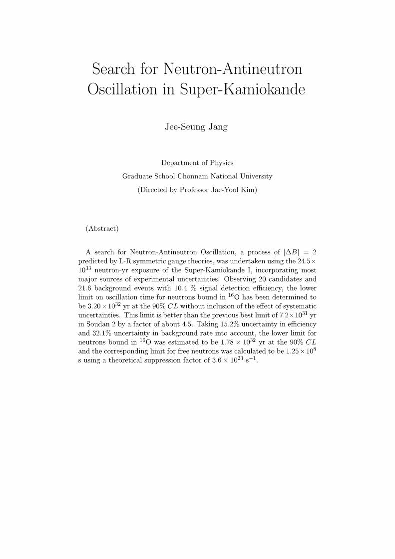
A search for Neutron-Antineutron Oscillation, a process of |∆B| = 2predicted by L-R symmetric gauge theories, was undertaken using the 24.5×1033 neutron-yr exposure of the Super-Kamiokande I, incorporating mostmajor sources of experimental uncertainties. Observing 20 candidates and21.6 background events with 10.4 % signal detection efficiency, the lowerlimit on oscillation time for neutrons bound in 16O has been determined tobe 3.20×1032 yr at the 90% CL without inclusion of the effect of systematicuncertainties. This limit is better than the previous best limit of 7.2×1031 yrin Soudan 2 by a factor of about 4.5. Taking 15.2% uncertainty in efficiencyand 32.1% uncertainty in background rate into account, the lower limit forneutrons bound in 16O was estimated to be 1.78 × 1032 yr at the 90% CLand the corresponding limit for free neutrons was calculated to be 1.25×108

s using a theoretical suppression factor of 3.6× 1023 s−1.

Chapter 1

Introduction

The Baryon Asymmetry of the Universe (BAU)[1][2] is one of the mostinteresting issues in particle physics and particle astrophysics. Baryon in-stability [3] in combination with CP violation and non-equilibrium thermo-dynamics in the early Universe , as first suggested by Sakharov, is the mostpopular explanation of BAU. In the early 1970, attempts at grand unificationof the fundamental interactions[4][5] led to the prediction of baryon numberas well as lepton number violation and even within the Standard Model itwas suggested baryon number was not conserved at the non-perturbativelevel[6]. Well established theories such as above have encouraged experi-mentalists to continue the search for baryon instability, even though directexperimental evidence supporting baryon number violation has not beenfound yet.

In the 1980’s, people began to be interested in experimental searches ofn − n oscillation (a process that was originally referred to neutron transi-tions) with |∆B| = 2 rather than usual nucleon decay of |∆B| = 1. It’s in-teresting to review the motivation behind first experimental search. In 1974,Georgi and Glashow made first predictions regarding observable nucleon de-cay modes with |∆B| = 1 such as p → e+π0, p → νK+ and p → µ+K0

which are favored in minimal SU(5) conserving B − L, which turn out tobe dominant modes in minimal SUSY SU(5). This model yields[7] partiallifetimes τp/B for p → e+π0 and p → νK+ are less than about 1035 yrand 1032 yr respectively but strictly suppresses processes with |∆B| = 2that violate B − L such as neutron-antineutron transition, the topic of thisdissertation. However, these predictions have been ruled out in recent yearsby experimental results. In particular, the lifetime limit for p → νK+, adominant mode of minimal SUSY SU(5), has been shown to be 2.3×1033 atthe 90%CL in published result of Super-Kamiokande[8]. As minimal SUSYSU(5) has been ruled out by stringent limits on |∆B| = 1 processes, it hasbecome important to study processes that obey different symmetry lawssuch as neutron-antineutron oscillation which can occur in large class of su-persymmetric SU(2)L

⊗SU(2)R

⊗SU(4)C [9] (Left-Right symmetric gauge

group).The n− n oscillation has the additional properties. The n− n oscillation

occurs at energies ∼ 105 GeV[10] compared to the unification scale of SU(5)∼ 1015−1016 GeV in which p → e+π0 would be observable with a lifetime ofabout 1034 yr. Thus, if n− n oscillation were to be observed experimentally,

1

new force of nature beyond the standard model would be discovered atthe energy scale above 1 TeV and an explanation of the matter-antimatterasymmetry would be put forward. If it were not to be discovered, it wouldprovide new limit on the stability of the neutrons.

There are two major experimental methods for an n− n searches: One ofthem is utilizing free neutrons from reactors or neutron spallation sourcessuch as the ILL at Grenoble[10] and the other method is monitoring neutronsbound inside the nuclei. In this thesis, neutrons bound in oxygen are studiedin Super-Kamiokande (Super-K). Figure 1.1[11] is showing the relationshipbetween the oscillation time limits of free neutron and bound neutron. Twomethods are related by theoretical ”nuclear suppression factor[12][13][14]”.

Super-Kamiokande is the world’s largest water Cherenkov detector witha net mass 50,000 tons located in Japan for observing neutrinos from var-ious natural sources such as the Sun, the Earth’s atmosphere, supernovaeand other astrophysical sources as well as neutrinos from artificial sourcessuch as particle beams. Many significant results were published from thefirst phase of Super-Kamiokande (called Super-K I) including the world’shighest limits on partial lifetimes for nucleon decay in minimal SUSY SU(5)under the condition of |∆B| = 1. n − n oscillation, a process of |∆B| = 2is studied in this thesis using the 91.7 kton-yr exposure of Super-K I. Eventhough searches for this process have been made in various nucleon decayexperiments including IMB[15], Kamiokande[16], Frejus[17] and Soudan[18],it has not to be observed yet. The current best limit for the n − n oscil-lation time for bound neutrons is TIron ≥ 7.2 × 1031 by Soudan 2 for ironnuclei. It has been expected that Super-Kamiokande will greatly improvethis limit because it has by far the world’s best neutron exposure, althoughthe Sudbury Neutrino Observatory[19] (SNO) is also planning on obtaininga competitive limit for bound neutrons.

In this thesis, n − n oscillation is studied using neutrons bound in oxy-gen nuclei corresponding to 24.5 × 1033 neutron-yr of Super-Kamiokandeoperating from April, 1996 to July, 2001 (the full Super-K I period). Be-fore describing the n− n analysis and result, I’ll outline the physics of n− nsearch and Super-K detector. MC simulation to estimate detection efficiencyof n− n oscillation and the number of background and detector simulationare described in Chapter4 and the reduction and reconstruction for Super-Kdata are described in Chapter5. In Chapter 6, data analysis methods, pro-cedure and result are described. And the final chapter, Chapter7, containsthe conclusions and suggestions for further research on this topic.

2

Figure 1.1: Current limits of n − n oscillation time. The horizontal axisrelates limit for free neutron oscillation time measured in reactor experi-ment and vertical axis for bound neutron oscillation time in nucleon decayexperiments. The bound neutron oscillation time is proportional to thefree neutron oscillation time squared with the constant being theoreticallydetermined, nuclear suppression factor.

3

Chapter 2

Physics of n− n Oscillation

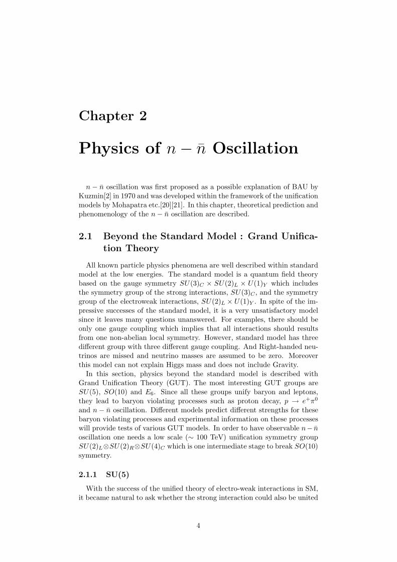
n− n oscillation was first proposed as a possible explanation of BAU byKuzmin[2] in 1970 and was developed within the framework of the unificationmodels by Mohapatra etc.[20][21]. In this chapter, theoretical prediction andphenomenology of the n− n oscillation are described.

2.1 Beyond the Standard Model : Grand Unifica-tion Theory

All known particle physics phenomena are well described within standardmodel at the low energies. The standard model is a quantum field theorybased on the gauge symmetry SU(3)C × SU(2)L × U(1)Y which includesthe symmetry group of the strong interactions, SU(3)C , and the symmetrygroup of the electroweak interactions, SU(2)L × U(1)Y . In spite of the im-pressive successes of the standard model, it is a very unsatisfactory modelsince it leaves many questions unanswered. For examples, there should beonly one gauge coupling which implies that all interactions should resultsfrom one non-abelian local symmetry. However, standard model has threedifferent group with three different gauge coupling. And Right-handed neu-trinos are missed and neutrino masses are assumed to be zero. Moreoverthis model can not explain Higgs mass and does not include Gravity.

In this section, physics beyond the standard model is described withGrand Unification Theory (GUT). The most interesting GUT groups areSU(5), SO(10) and E6. Since all these groups unify baryon and leptons,they lead to baryon violating processes such as proton decay, p → e+π0

and n− n oscillation. Different models predict different strengths for thesebaryon violating processes and experimental information on these processeswill provide tests of various GUT models. In order to have observable n− noscillation one needs a low scale (∼ 100 TeV) unification symmetry groupSU(2)L⊗SU(2)R⊗SU(4)C which is one intermediate stage to break SO(10)symmetry.

2.1.1 SU(5)

With the success of the unified theory of electro-weak interactions in SM,it became natural to ask whether the strong interaction could also be united

4

with the weak and electromagnetic interactions into a single. The basic ideaof the approach to a universal coupling is illustrated in Figure 2.1.

Figure 2.1: Running coupling constants g, g’ and gs of the electro-weak andstrong interactions appear to extrapolate to a single value at q ∼ 1015 GeV.

The graph indicates the dependence on momentum transfer, or mass scale,of the running coupling constants for the Abelian U(1) field described byg′, for the non-Abelian SU(2) field denoted by g, and for the non-AbelianSU(3) color field which we denote gs (where αs = gs

2/4π). As q increases, g′

increases slightly while g decreased slightly and gs decreased more quickly.It is a remarkable fact that when all three interactions are extrapolated,they appear to meet at a single point at the colossal value of q ' 1015 GeV.(There are numerical constants of order unity multiplying g, g′ and gs, whichwe have omitted from Figure 2.1. Implicit in this enormous extrapolationis the bold assumption that Nature has run out of ideas and has no newsurprises in the range from q ' 30 GeV/c of present accelerator experiments,all the way to q ' 1015 GeV/c. There may instead be new internal degreesof freedom, quark or lepton substructure, only just around the corner andto be revealed at the next generation of accelerators. On the basis of pastexperience, one would think that this is rather likely.

There are many ways in which the SU(2), U(1) and SU(3) symmetriescould be incorporated into a more global gauge symmetry. The simplestgrand unifying symmetry is that of the group SU(5)-Georgi and Glashow,1974. This incorporates the known fermions (leptons and quarks) in mul-tiplets, inside which quarks can transform to leptons, and quarks to anti-quarks, via the mediation of very massive (1015 GeV) bosons Y and X, withelectric charges -1/3 and -4/3 respectively. There are a total of 24gaugebosons in the model. These consist of the 8 gluons of SU(3) and the W±, Z0

and photon of SU(2)×U(1), plus the 12 varieties of X and Y boson (each car-rying 3 colors and existing in particle and antiparticle states). The fermions(quarks and leptons) are assigned to different ”generations”, The first gener-

5

ation consists of 15 states: the u- and d-quarks, each in 3 color and 2 helicitystates; the e− with 2 helicity states; and the νe, with 1 helicity only. Byconvention, we write them down as LH states, since, for example, the e−RH

state and the e+LH state are equivalent (by CP). The 15 states comprise

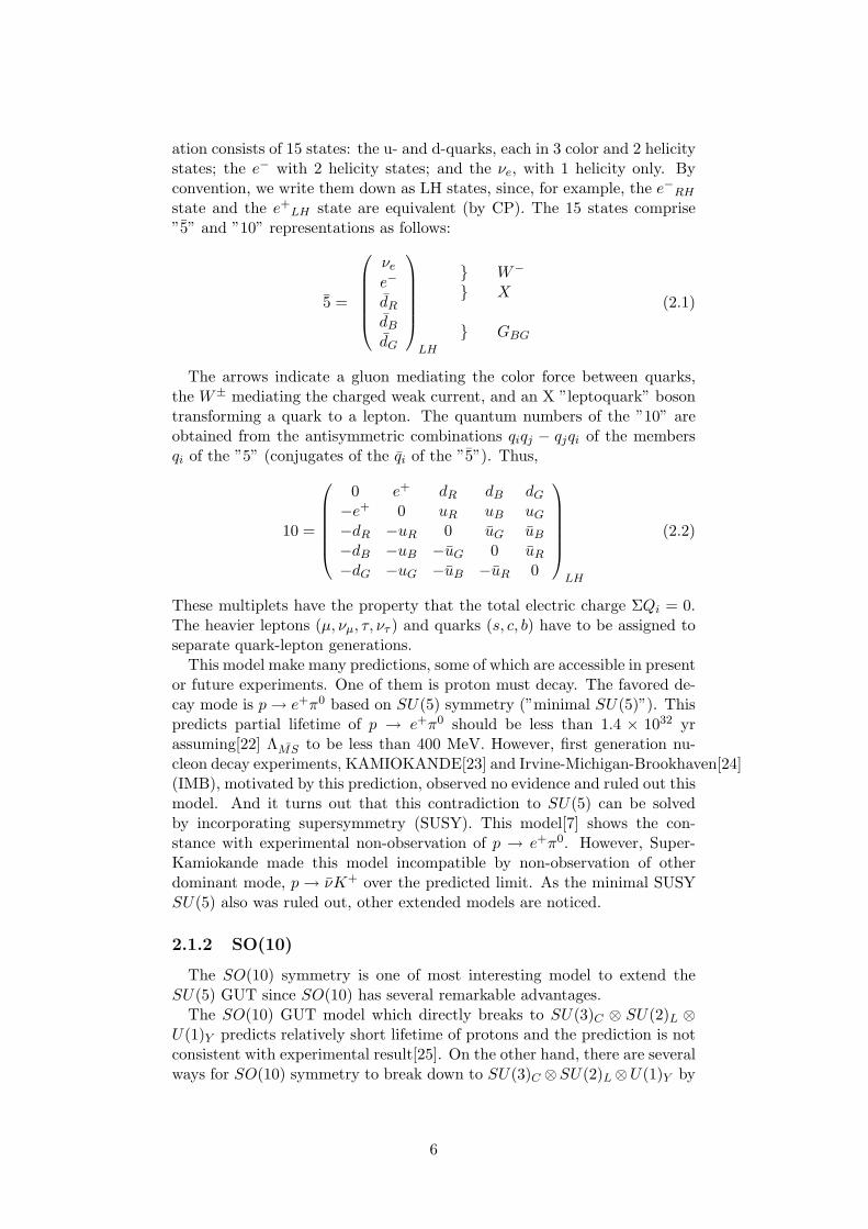
”5” and ”10” representations as follows:

5 =

νe

e−

dR

dB

dG

LH

}}

}

W−

X

GBG

(2.1)

The arrows indicate a gluon mediating the color force between quarks,the W± mediating the charged weak current, and an X ”leptoquark” bosontransforming a quark to a lepton. The quantum numbers of the ”10” areobtained from the antisymmetric combinations qiqj − qjqi of the membersqi of the ”5” (conjugates of the qi of the ”5”). Thus,

10 =

0 e+ dR dB dG

−e+ 0 uR uB uG

−dR −uR 0 uG uB

−dB −uB −uG 0 uR

−dG −uG −uB −uR 0

LH

(2.2)

These multiplets have the property that the total electric charge ΣQi = 0.The heavier leptons (µ, νµ, τ, ντ ) and quarks (s, c, b) have to be assigned toseparate quark-lepton generations.

This model make many predictions, some of which are accessible in presentor future experiments. One of them is proton must decay. The favored de-cay mode is p → e+π0 based on SU(5) symmetry (”minimal SU(5)”). Thispredicts partial lifetime of p → e+π0 should be less than 1.4 × 1032 yrassuming[22] ΛMS to be less than 400 MeV. However, first generation nu-cleon decay experiments, KAMIOKANDE[23] and Irvine-Michigan-Brookhaven[24](IMB), motivated by this prediction, observed no evidence and ruled out thismodel. And it turns out that this contradiction to SU(5) can be solvedby incorporating supersymmetry (SUSY). This model[7] shows the con-stance with experimental non-observation of p → e+π0. However, Super-Kamiokande made this model incompatible by non-observation of otherdominant mode, p → νK+ over the predicted limit. As the minimal SUSYSU(5) also was ruled out, other extended models are noticed.

2.1.2 SO(10)

The SO(10) symmetry is one of most interesting model to extend theSU(5) GUT since SO(10) has several remarkable advantages.

The SO(10) GUT model which directly breaks to SU(3)C ⊗ SU(2)L ⊗U(1)Y predicts relatively short lifetime of protons and the prediction is notconsistent with experimental result[25]. On the other hand, there are severalways for SO(10) symmetry to break down to SU(3)C ⊗SU(2)L⊗U(1)Y by

6

two steps[26].

SO(10) →

SU(5)⊗ U(1)SU(4)⊗ SU(2)L ⊗ SU(2)R

SU(3)⊗ SU(2)L ⊗ SU(2)R ⊗ U(1)SU(3)⊗ SU(2)L ⊗ U(1)⊗ U(1)

→ SU(3)C⊗SU(2)L⊗U(1)Y

(2.3)One of advantages of SO(10) GUT models is that it can contain the left-right symmetry which is missed in the standard electroweak model. Secondadvantage is that SO(10) model has representations of 16 in which there isa room for right handed neutrinos(νR) missed in the SU(5) model. SO(10)model that implements the seesaw mechanism[27] may explain the neutrinomasses and mixing. Moreover, the fermion unification into a single repre-sentation of 16 is a attractive feature of the model.

SO(10) models predict sin2θW consistent with experimental results andthe running coupling constants can meet at a single unification point[28][29].Among several intermediate symmetries, SU(4)⊗ SU(2)L ⊗ SU(2)R whichwas suggested by Pati and Salam[4] in 1973 is very interesting because itcontains the left-right symmetry. Within this framework, an immediate im-plication of (B−L)-symmetry breaking is the existence not only of Majorananeutrinos (∆L = 2 in the lepton section) but also the new phenomenon ofn → n transition (∆B = 2 in the hadron sector), which we call ”neutronoscillations”[20].

2.2 Prediction for n − n Oscillation in L-R Sym-metric Gauge Theory

There are many models for n − n oscillation. Among them, SU(2)L ×SU(2)R×SU(4)C which SU(4) unifies color and B−L symmetry is adoptedin this section. Following prediction for n− n oscillation within this frame-work is from Mohapatra[10].

Lifetime of n−n oscillation for free neutrons is led with observable strengthdepends on the details of the theory such as value of mass scales etc.

τn−n =h

2πδmn−n(2.4)

where h is Plank’s constant and δmn−n is the transition mass for n → ntransition. Within the framework of ”partial unification” group SU(2)L ×SU(2)R×SU(4)C for electroweak and strong interactions, in order to obtainn− n oscillation process, the gauge symmetry breaking of the model has tobe broken by the Higgs multiplets as in Ref.[21]: A bidoublet, φ(2,2,1),and a pair of triplets, ∆L(3, 1, 10) + ∆R(1, 3, 10). The quarks and leptonsare assigned to representations as follows: QL(2, 1, 4) + QR(1, 2, 4). Hereleptons are considered as the fourth color. The allowed Yukawa couplingsin the model are given by:

LY = yqQLφQR + f(QLQL∆L + QRQR∆R) + h.c. (2.5)

Here all generation indices was omitted and the couplings symbolically omit-ting charge conjugation matrices, Pauli matrices etc was denoted. The Higgs

7

potential of the model can be easily written down; the term in it which is in-teresting for the purpose of this study is λεijklεi′j′k′l′∆L,ii′∆L,jj′∆L,kk′∆L,ll′+L → R + h.c..

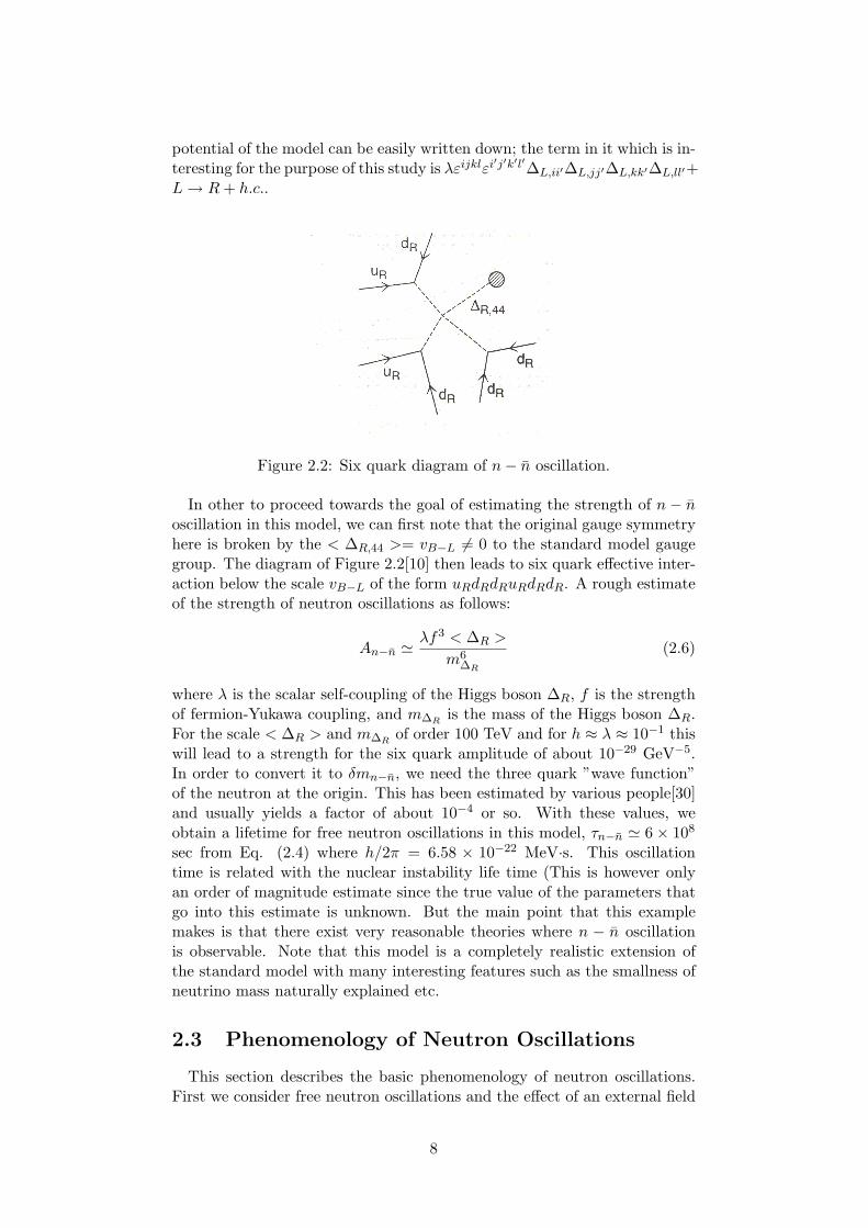
Figure 2.2: Six quark diagram of n− n oscillation.

In other to proceed towards the goal of estimating the strength of n − noscillation in this model, we can first note that the original gauge symmetryhere is broken by the < ∆R,44 >= vB−L 6= 0 to the standard model gaugegroup. The diagram of Figure 2.2[10] then leads to six quark effective inter-action below the scale vB−L of the form uRdRdRuRdRdR. A rough estimateof the strength of neutron oscillations as follows:

An−n ' λf3 < ∆R >

m6∆R

(2.6)

where λ is the scalar self-coupling of the Higgs boson ∆R, f is the strengthof fermion-Yukawa coupling, and m∆R

is the mass of the Higgs boson ∆R.For the scale < ∆R > and m∆R

of order 100 TeV and for h ≈ λ ≈ 10−1 thiswill lead to a strength for the six quark amplitude of about 10−29 GeV−5.In order to convert it to δmn−n, we need the three quark ”wave function”of the neutron at the origin. This has been estimated by various people[30]and usually yields a factor of about 10−4 or so. With these values, weobtain a lifetime for free neutron oscillations in this model, τn−n ' 6× 108

sec from Eq. (2.4) where h/2π = 6.58 × 10−22 MeV·s. This oscillationtime is related with the nuclear instability life time (This is however onlyan order of magnitude estimate since the true value of the parameters thatgo into this estimate is unknown. But the main point that this examplemakes is that there exist very reasonable theories where n − n oscillationis observable. Note that this model is a completely realistic extension ofthe standard model with many interesting features such as the smallness ofneutrino mass naturally explained etc.

2.3 Phenomenology of Neutron Oscillations

This section describes the basic phenomenology of neutron oscillations.First we consider free neutron oscillations and the effect of an external field

8

on neutron oscillations is treated. In particular the effect of an external mag-netic field on the opposite magnetic momentum of n and n. This descriptionis by R. N. Mohapatra and R. E. Marshak[31]

2.3.1 Free Neutron Oscillations

The starting point is the n− n mass matrix.

Lmass = ψMψ (2.7)

where

ψ =

(nn

)

and

M =

(A δmδm A

)(2.8)

In Eq. (1.8), δm is the ∆B = 2 transition mass between n and n states.The equality of the diagonal elements follows from CPT invariance and thatof the off-diagonal elements from CP invariance. The eigenstates of M canbe written as:

n1,2 =n± n√

2(2.9)

with masses:m1,2 = A± δm (2.10)

Next, the amplitude for finding an n at time t starting with a beam of neu-trons at t=0 is:

|n(t) >= e−γt2

(|n1(0) > e−im1t + |n2(0) > e−im2t

√2

)(2.11)

where we have assumed that the decay widths of n1 and n2 are equal anddenoted by γ. The probability for finding an n at time t, Pn(t) is:

Pn(t) =e−γt

2(1− cos2δmt) (2.12)

If t << 1/γm, then we obtain:

Pn(t) ' e−γt(δmt)2 (2.13)

The upper limit on δm can be estimated from the upper limit on the ∆B = 2”bound” nucleon transition rate, Γ∆B=2 by means of the relation:

δm '√

Γ∆B=2M (2.14)

Here, M is a typical hadronic mass. This part will be explained again inChapter 6.3.2. Anyway, it follows that if a beam of N free neutrons is allowedto travel for a time T before hitting a target, the number of antineutrons,N , at the target after T should be (assuming γT << 1):

N ≤ N(T

τn−n)2 (2.15)

9

τn−n is n − n oscillation time. With reasonable values of N and T , aboveequation would be rather promising for a ”free” neutron oscillation exper-iment. However, there is a complicating factor resulting from the presenceof the earth’s magnetic field which shifts the energy of n and n by oppositeamounts ±µB ∼ 10−11 eV, which is much larger than δm. We deal withthis situation in the next section.

2.3.2 Oscillation of Neutrons in an External Field

If the neutron oscillation takes place in an external field (such as theearth’s magnetic field or other field) so that the CPT theorem need not berespected, the picture outlined in previous section changes and we have:

M =

(A1 δmδm A2

)(2.16)

The neutron mass eigenstates in this case are:

|n1 >' |n > +θ|n >

|n2 >' −θ|n > +|n >

whereθ ' δm/∆M (2.17)

where ∆M ≡ M1 −M2 ≈ A1 −A2 >> δm. And probability is:

Pn(t) ' θ2

2[1− cos∆Mt] (2.18)

Above equation is interesting in two limiting cases: (a) ∆Mt >> 1 and (b)∆Mt << 1. In case (a), the second term oscillates rapidly and the averageprobability for finding an n, < Pn >av becomes:

< Pn >av' (δm

∆M)2 (2.19)

In case (b), we get:Pn(t) ' (δmt)2 (2.20)

as long as γt << 1.

10

Chapter 3

Super-Kamiokande

Super-Kamiokande is the world’s largest water Cherenkov detector witha net mass 50,000 tons located in Muzumi mine, Gifu, Japan. Detectorcavity lies under the peak of Mt. Ikenoyama with 1,000 meters of rockor 2,700 meter-water-equivalent mean overburden. The scientific goal ofthis experiment is observing neutrinos from various natural sources suchas the Sun, the Earth’s atmosphere, supernovae and other astrophysicalsources as well as neutrinos from artificial sources such as particle beamsand includes nucleon decay search. Super-Kamiokande began to take data inApril, 1996. This operating was shut down for maintenance and upgrade inJuly, 2001. This running period is referred to as Super-Kamiokande I (Super-K I). During refilling the water to start Super- Kamiokande II, in November,2001, an apparent cascade of implosions triggered by a single photomultipliertube (PMT) implosion destroyed over half of the PMTs installed in thedetector. In 2002, the detector was reconstructed with 5,000 PMTs (theoriginal number of PMTs used in Super-K is 11,146) encased in acrylic coversto avoid a similar accident. After partial reconstruction, Super-KamiokandeII was operated from Dec. 2002 to Oct. 2005 with temporarily reduced PMTcoverage (47% of Super-K I). In June 2006, the third phase experiment,Super-Kamiokande III, has been started after full reconstruction recoveringPMT coverage as Super-K I. In this thesis, 4.07 years data in Super-K Iperiod is used for analysis. The configuration and operational characteristicsof the detector in the Super-K I period are described in this chapter basedon [32].

3.1 Cherenkov Radiation

The Super-Kamiokande is water Cherenkov detector which observed rela-tivistic charged particles in water by detecting the Cherenkov light. Cherenkovphotons are radiated when a charged particle in a material medium movesfaster than the speed of light in that same medium. Therefore a particleemitting Cherenkov radiation must have a velocity

vparticle ≥ c

n(3.1)

where n is the index of refraction and c is the speed of light in a vacuum[33].The momentum threshold of Cherenkov radiation is determined by the re-

11

Figure 3.1: Cherenkov radiation.

fractive index of the medium and the mass of particle. In water, the refrac-tive index is about 1.34, and the momentum threshold for electrons, muonsand pions are 0.57, 118 and 156 MeV/c, respectively.

This radiation creates electromagnetic shock wave. This is illustratedin Figure 3.1. The coherent wave front formed in conical in shape and isemitted at a well-defined angle

cosθC =1

nβ(3.2)

with respect to the trajectory of the particle where β = v/c and this angleis called as Cherenkov angle. For the particle with β ' 1 in water, theCherenkov angle is about 42o. This angle is dependent on the speed of theparticles and the frequency of the emitted radiation.

The number of photons emitted by Cherenkov radiation is given as afunction of the wave length λ as follows;

d2N

dxdλ=

2πα

λ2(1− 1

n2β2) (3.3)

where x is the path length of the charged particle and α is the fine struc-ture constant. About 340phtons/cm are emitted between the wavelengthof 300nm to 600nm, which is the sensitive wavelength region of photomul-tiplier tubes. Particle emitting Cherenkov light project ring images on thewall inside of the detector. Figure 3.2 shows display of a typical neutrinoevent in the Super-Kamiokande detector.

3.2 Detector

3.2.1 Water Tank

Figure 3.3 shows the schematic view of detector. The outer shell of thedetector is a cylindrical stainless steel tank, 39 m in diameter and 42m inheight. The tank is self-supporting, with concrete backfilled against the

12

Figure 3.2: Neutrino event display in the Super-Kamiokande.

rough-hewn stone walls to counteract water pressure when the tank is filledwith water. The capacity of the tank exceeds 50 ktons of water. A cylindricalPMT support structure divides the tank into two distinct, optically isolatedvolumes. The structure has inner dimensions, 33.8 m (diameter) by 36.2m (height), defining the inner detector (ID) which contains 32 ktons ofwater and was viewed by inward-facing 50 cm (20 inch) PMTs (HamamatsuR3600). Approximately 2.5 m distance remains on all outside of the supportstructure. This outside region defining outer detector (OD), serves as anactive veto counter against incoming particles as well as a passive shield forneutrons and gamma rays from the surrounding rocks. OD was instrumentedwith 1,885 outward-facing 20 cm (8 inch) PMTs (Hamamatsu R1408). Thetwo detector volumes are isolated from each other by two light-proof sheetson both surfaces of the PMT support structure. The 55 cm thick supportstructure comprises dead space from which light in principle cannot escape.Therefore, any interaction in that space cannot be detected. The OD PMTswere mounted in water-proof housings which effectively block light from thedead space. However, because the ID PMTs were not fully covered in back,some light generated in this region was still detected by the ID PMTs.

3.2.2 Photomultiplier Tubes

Inner Detector Photomultiplier Tubes

A 50 cm ID PMTs used in this experiment is described in Figure 3.4and the specifications are summarized in Table 3.1. The bialkali (Sb-K-Cs)photocathode has peak quantum efficiency of about 21% at 360 nm-400 nmas shown in Figure 3.5. The collection efficiency for photoelectrons (pe) atthe first dynode is over 70%. The transit time spread for a 1 pe signal is

13

Figure 3.3: Schematic view of Super-Kamiokande.

2.2 ns. The average dark noise rate at the 0.25 pe threshold is about 3 kHzin Super-Kamiokande I. The ID PMTs were operated with gain of 107 at asupply high voltage ranging from 1700 to 2000 V. The neck of each PMTwas coated with a silver reflector to block external light.

Outer Detector Photomultiplier Tubes

These PMTs were first adopted in the IMB experiment[34] and they arereused in the Super-Kamiokande after finishing that experiment. Light col-lection efficiency in the OD PMTs is enhanced by wavelength shifting (WS)plates attached to each OD PMT. The WS plates are square acrylic panels,60 cm on a side and 1.3 cm thick, doped with 50 mg/l of bis-MSB. The WSplates function by absorbing UV light, and then re-radiating photons in theblue-green, better matching the spectral sensitivity of the PMT’s bialkaliphotocathode. The light collection of the PMT plus WS unit is improvedover that of the bare PMT by about a factor of 1.5.

14

Figure 3.4: Schematic view of a 50 cm PMT.

Shape HemisphericalPhotocathode area 50 cm diameterWindow material Pyrex glass (4 ∼ 5 mm)Photocathode material Bialkali (Sb-K-Cs)Quantum efficiency 22% at λ=390 nmDynodes 11 stage Venetian blind typeGain 107 at ∼ 2000 VDark current 200 nA at 107 gainDark pulse rate 3kHz at 107 gainCathode non-uniformity < 10 %Anodes non-uniformity < 40 %Transit time 90 nsec at 107 gainTransit time spread 2.2 nsec (1 σ) for 1 p.e. equivalent signalsWeight 13 kgPressure tolerance 6 kg/cm2 water proof

Table 3.1: Specification of a 50 cm PMT.

15

Figure 3.5: Quantum efficiency of the photocathode as a function of wave-length.

3.2.3 PMT Support Structure and Others

Figure 3.6 shows a detail of the PMT support structure. All supportstructure components are stainless steel. The basic unit for the ID PMTsis a supermodule, a frame which supports a 3x4 array of PMTs. Eachsupermodule has two OD PMTs attached on its back side. Opaque blackpolyethylene telephthalate sheets cover the gaps among the PMTs in the IDsurface. These sheets improve the optical separation between the ID andOD and suppress unwanted low-energy events due to residual radioactivityoccurring behind the PMTs.

Light collection efficiency is enhanced by WS as mentioned in previoussection. To further enhance light collection, the OD volume is lined witha reflective layer made from Type 1073B Tyvek manufactured by DuPont.This inexpensive and very tough paper-like material has excellent reflectiv-ity in the wavelength range in which PMTs are most sensitive, especiallyat short wavelengths. Measured reflectivities are on the order of 90% forwavelengths in excess of 400 nm, falling to 80% at about 340 nm[35]. Thepresence of this liner allows multiple reflections of Cherenkov light, whichminimizes the effects of dead PMTs, given their coarse spacing in the OD.Cherenkov light is spread over many PMTs, reducing pattern resolution butincreasing overall detection efficiency.

To protect against low energy background from radon decay productsin the air, the roof of the cavity and the access tunnels were sealed with acoating called Mineguard produced by Urylon in Canada. In addition,doubledoors in the access tunnels restrict air flow from the mine into the detec-tor cavern and ”radon-free” air is supplied and radon-reduced air is alsoproduced in the mine.

The average geomagnetic field is about 450 mG and is inclined by about

16

Figure 3.6: Schematic view of PMT support structure.

17

45o with respect to the horizon at the detector site. The strength anduniform direction of the geomagnetic field could systematically bias photo-electron trajectories and timing in the PMTs. To counteract this, 26 setsof horizontal and vertical Helmholtz coils are arranged around the innersurfaces of the tank. With operation of these coils, the average field in thedetector is reduced to about 50 mG. The magnetic field at various PMTlocations were measured before the tank was filled with water.

3.2.4 Water Purification

Super-Kamiokande should keep the water transparency as high as pos-sible removing small dust, metal ions like Fe, Ni, Co and bacteria in thewater. And radioactive material, mainly Rn, Ra and Th, can be source ofbackground. Especially, radon is serious background for the solar neutrinoanalysis. However, since there is ∼ 60 cm space between the surface of thewater and the top of the water tank, radon gas contaminated in the air inthe gap could dissolve in the water. Therefore, the 50 ktons of purified wa-ter in the Super-Kamiokande tank is continuously reprocessed at the rate ofabout 30 tons/hour in this closed cycle system. In the Kamioka mine, thereis clean water flowing near the detector and it can be used freely in largequantities. This water is circulated through the water purification systemshown in Figure 3.7. The water purification system consists of the followingcomponents;

• 1µm Filter

• Heat exchanger : The water temperature rises due to the heat gener-ated by pumps and PMTs. The temperature is kept at around 14oCto suppress bacteria growth.

• Ion exchanger : This removes metal ions in the water.

• Ultra-Violet sterilize : This kills bacteria. The documentation statesthe number of bacteria can be reduced to less than 103 ∼ 104/100ml.

• Vacuum degasifier : This removes gas resolved in the water. It is ableto remove about 99% of the oxygen gas and 96% of the radon gas.

• Cartridge polisher : This is a high performance ion exchanger.

• Ultra filter : This remove small dust even of the order of nanometers.

The typical number of particles larger than 0.2µm is reduced to 6 particle/ccafter purification.

3.2.5 Electronics and Data Acquisition System

Inner Detector Electronics and Data Acquisition

ID PMT signals are processed by custom built TKO modules called Analog-Timing-Modules (ATMs). The TKO (TRISTAN KEK Online) system wasoriginally developed and built by KEK, and is optimized for front-end elec-tronics where a large number of channels are to be handled. The ATMhas the functionality of a combined ADC (Analog-to-Digital Converter) andTDC (Time-to-Digital Converter), and records the integrated charge and

18

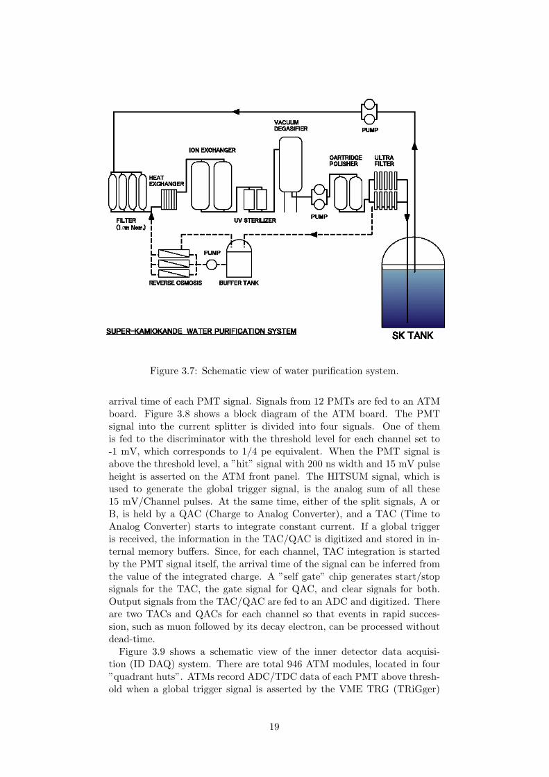
Figure 3.7: Schematic view of water purification system.

arrival time of each PMT signal. Signals from 12 PMTs are fed to an ATMboard. Figure 3.8 shows a block diagram of the ATM board. The PMTsignal into the current splitter is divided into four signals. One of themis fed to the discriminator with the threshold level for each channel set to-1 mV, which corresponds to 1/4 pe equivalent. When the PMT signal isabove the threshold level, a ”hit” signal with 200 ns width and 15 mV pulseheight is asserted on the ATM front panel. The HITSUM signal, which isused to generate the global trigger signal, is the analog sum of all these15 mV/Channel pulses. At the same time, either of the split signals, A orB, is held by a QAC (Charge to Analog Converter), and a TAC (Time toAnalog Converter) starts to integrate constant current. If a global triggeris received, the information in the TAC/QAC is digitized and stored in in-ternal memory buffers. Since, for each channel, TAC integration is startedby the PMT signal itself, the arrival time of the signal can be inferred fromthe value of the integrated charge. A ”self gate” chip generates start/stopsignals for the TAC, the gate signal for QAC, and clear signals for both.Output signals from the TAC/QAC are fed to an ADC and digitized. Thereare two TACs and QACs for each channel so that events in rapid succes-sion, such as muon followed by its decay electron, can be processed withoutdead-time.

Figure 3.9 shows a schematic view of the inner detector data acquisi-tion (ID DAQ) system. There are total 946 ATM modules, located in four”quadrant huts”. ATMs record ADC/TDC data of each PMT above thresh-old when a global trigger signal is asserted by the VME TRG (TRiGger)

19

Figure 3.8: A block diagram of ATM board used for inner detector dataacquisition.

Figure 3.9: The data acquisition system for the inner detector.

20

Figure 3.10: Outer detector DAQ block diagram and data flow.

module. The global trigger signal and event number information generatedin the TRG module, are distributed to all ATMs via 48 GONG (Go/NoGo)modules.

Outer Detector Electronics and Data Acquisition

A block diagram of the OD data acquisition (OD-DAQ) system is shown inFigure 3.10. As with the inner detector, signals from the PMTs are processedand digitized in each of 4 quadrant electronics huts. From there, the signalsare picked off, digitized and stored. As in the ID, local HITSUM pulsesare formed in each quadrant hut and sent to the central hut, where theiranalog sum creates an OD trigger signal when the OD HITSUM thresholdis exceeded. Figure 3.10 illustrates the data flow in a quadrant hut as wellas the overall data flow. When a trigger from any source occurs, the dataare passed out of the quadrant huts to the central hut for further processing.Once the PMT signals have been picked off, coaxial ribbon cables feed themto the custom charge-to-time conversion modules (QTC). The purpose ofthese modules is to measure the hit time and charge of the PMT pulse andconvert it to a form which can be easily read and stored by the time-to-digital converters (TDCs). The output of the QTC modules is a logic pulse(ECL level) whose leading edge marks the hit arrival time and whose widthrepresents the integrated charge Q of the PMT pulse.

21

Figure 3.11: Relative photo-sensitivity. (a) Measurement result, (b) Defini-tion of the incident angle.

3.3 Calibrations

3.3.1 Water Transparency Measurement

Indirect Measurement with Cosmic Rays

The light attenuation length in water can be measured by using through-going cosmic ray muons. These muons are energetic enough to deposit al-most constant ionization energy per unit path length (about 2 MeV/cm) in-dependent of particle energy. This fact makes it possible to use these muonsas a ”constant” light source. The advantage of this method is that contin-uous and abundant samples of muons come without cost as we take normaldata. The disadvantage is that we cannot measure the transparency as afunction of wavelength. However, since what we measure is the Cherenkovspectrum, this disadvantage is not necessarily a problem. Under the assump-tion that light reaching the PMTs is not scattered, the charge Q observedby a PMT is expressed by

Q = Q0f(θ)

lexp(− l

L) (3.4)

Where l is the light path length, L the effective attenuation length, Q0 aconstant and f(θ) the relative photo-sensitive area, which depends upon theincidence angle θ of the light on the PMT, as shown in Figure 3.11. Figure3.12 is as a function of the path length l together with the best fit in the formof the function defined above. The resulting attenuation length is found tobe 105.4±0.5 m.

As the data sample for this measurement is accumulated automaticallywhile we take normal data, it is possible to continuously monitor the at-tenuation length as a function of time. Figure 3.13 shows the attenuationlength changes with time, which are correlated with water quality. Suchtime variations in the attenuation length are corrected in analysis from thetime series of calibration data.

22

Figure 3.12: Effective charge observed as a function of the path length.

Figure 3.13: Time variation of the water attenuation length measured bythrough-going.

23

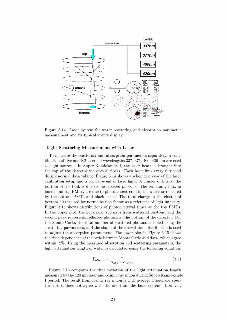
Figure 3.14: Laser system for water scattering and absorption parametermeasurement and its typical events display.

Light Scattering Measurement with Laser

To measure the scattering and absorption parameters separately, a com-bination of dye and N2 lasers of wavelengths 337, 371, 400, 420 nm are usedas light sources. In Super-Kamiokande I, the laser beam is brought intothe top of the detector via optical fibers. Each laser fires every 6 secondduring normal data taking. Figure 3.14 shows a schematic view of the lasercalibration setup and a typical event of laser light. A cluster of hits at thebottom of the tank is due to unscattered photons. The remaining hits, inbarrel and top PMTs, are due to photons scattered in the water or reflectedby the bottom PMTs and black sheet. The total charge in the cluster ofbottom hits is used for normalization factor as a reference of light intensity.Figure 3.15 shows distributions of photon arrival times at the top PMTs.In the upper plot, the peak near 730 ns is from scattered photons, and thesecond peak represents reflected photons at the bottom of the detector. Forthe Monte Carlo, the total number of scattered photons is tuned using thescattering parameters, and the shape of the arrival time distribution is usedto adjust the absorption parameters. The lower plot in Figure 3.15 showsthe time dependence of the ratio between Monte Carlo and data, which agreewithin 2%. Using the measured absorption and scattering parameters, thelight attenuation length of water is calculated using the following equation.

Lattenu =1

αabs + αscatt(3.5)

Figure 3.16 compares the time variation of the light attenuation lengthmeasured by the 420 nm laser and cosmic ray muon during Super-KamiokandeI period. The result from cosmic ray muon is with average Cherenkov spec-trum so it does not agree with the one from the laser system. However,

24

Figure 3.15: The upper plot is the photon arrival time distribution of thetop PMTs. Dots is data and line is Monte Calro. The lower plot is the ratio,(MC-DATA)×100/DATA.

Figure 3.16: Time variation measured light attenuation length since Novem-ber 1999, using the laser system (triangles) and cosmic ray muons (crosses).

25

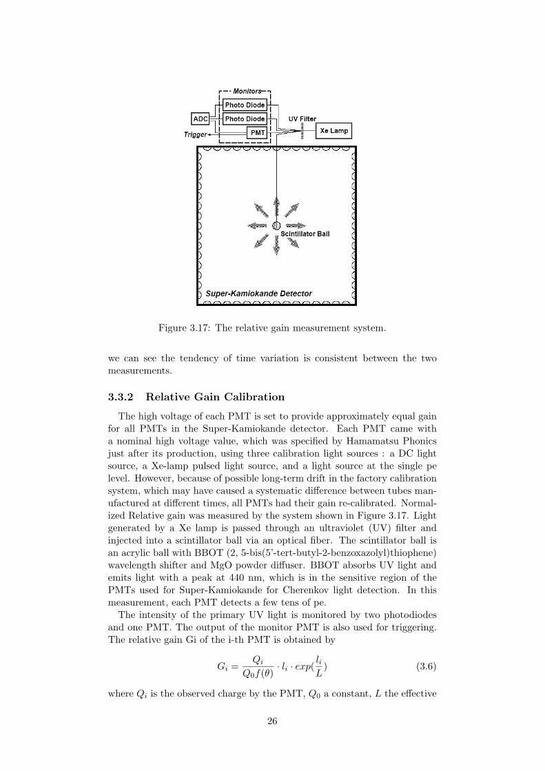
Figure 3.17: The relative gain measurement system.

we can see the tendency of time variation is consistent between the twomeasurements.

3.3.2 Relative Gain Calibration

The high voltage of each PMT is set to provide approximately equal gainfor all PMTs in the Super-Kamiokande detector. Each PMT came witha nominal high voltage value, which was specified by Hamamatsu Phonicsjust after its production, using three calibration light sources : a DC lightsource, a Xe-lamp pulsed light source, and a light source at the single pelevel. However, because of possible long-term drift in the factory calibrationsystem, which may have caused a systematic difference between tubes man-ufactured at different times, all PMTs had their gain re-calibrated. Normal-ized Relative gain was measured by the system shown in Figure 3.17. Lightgenerated by a Xe lamp is passed through an ultraviolet (UV) filter andinjected into a scintillator ball via an optical fiber. The scintillator ball isan acrylic ball with BBOT (2, 5-bis(5’-tert-butyl-2-benzoxazolyl)thiophene)wavelength shifter and MgO powder diffuser. BBOT absorbs UV light andemits light with a peak at 440 nm, which is in the sensitive region of thePMTs used for Super-Kamiokande for Cherenkov light detection. In thismeasurement, each PMT detects a few tens of pe.

The intensity of the primary UV light is monitored by two photodiodesand one PMT. The output of the monitor PMT is also used for triggering.The relative gain Gi of the i-th PMT is obtained by

Gi =Qi

Q0f(θ)· li · exp(

liL

) (3.6)

where Qi is the observed charge by the PMT, Q0 a constant, L the effective

26

light attenuation length, li the distance from the light source to the PMTand f(θ) the relative photo-sensitivity as a function of the incident angleof light a on the PMT defined in Figure 3.11. The high voltage value foreach PMT is set so that the ”corrected Q” of each PMT is approximatelythe same as for all the others. Here, ”corrected Q” is the pulse heightcorrected for light attenuation, acceptance of the PMT, and uniformity ofthe scintillator ball. It is further normalized by the Xe monitor pulse height.This measurement is done for various positions of the scintillator ball andsettings of the high voltage value. After the initial gain adjustment, longterm stability of PMT gain was monitored using the same system. Theabsolute value of PMT gain cannot be measured while the experiment isrunning. The relative gain spread gain is defined as the standard deviationobtained by fitting the relative gain distribution of all PMTs to a Gaussian.It was 7.0% at the beginning of Super-Kamiokande I.

3.3.3 Relative Timing Calibration

The relative timing of PMT hits is important for event reconstruction. Itdepends on the length of the signal cable between the PMT and the ATM,and also depends on observed charge because of the discriminator slewingeffect. The timing difference in each individual PMT has to be measuredprecisely to get better timing resolution. Figure 3.18 shows the system formeasuring the relative timing of hit PMTs. The N2 laser emits intenselight of wavelength 337 nm within a very short time (less than 3 ns). Thewavelength is shifted to 384 nm, which is near the lower edge of sensitivityof a PMT to the Cherenkov light, by a dye laser module. The light intensityis changed by an optical filter, and the PMT timing is measured at variouspulse heights. After passing through the optical filter, the light goes to thediffuser ball in the detector through an optical fiber. The schematic viewof the diffuser ball is also shown in Figure 3.18. The diffuser tip located atthe center of the ball is made from TiO2 suspended in optical cement. Thelight emitted from the tip is further diffused by LUDOX manufactured byGrace Davison, silica gel made of 20 nm glass fragments. The combination ofdiffuser tip and LUDOX make modestly diffused light without introducingsignificant timing spread. A typical scatter plot of the timing and pulseheight is shown in Figure 3.19, which is called a ’TQ-map’. Each PMT hasits own TQ-map, which is applied in data reduction. The timing resolutionof PMTs as a function of pulse height is estimated from the TQ maps.Typical timing resolution at the single pe level is better than 3 ns.

3.3.4 Other Calibrations

There are other calibrations using stopping muon, neutral pion, LINAC,etc. The detail of the other calibrations can be found in [32].

27

Figure 3.18: The timing calibration system.

Figure 3.19: A typical plot of timing vs. pulse height. This plot is referredas ’TQ-map’.

28

Chapter 4

Simulation

We simulate not only the n− n oscillation but also the background eventssince background is pivotal component of a search for a rare process suchas nucleon decay or transition. Atmospheric neutrino interactions with anaverage energy of 1∼3 GeV are most significant source of background forn−n oscillation as well as nucleon decay. We use same 100 years atmosphericneutrino MC that has been used for neutrino oscillation study in Super-Kamiokande I of 4.07 years livetime. In this chapter, I outline the physicalassumptions including those related to kinematics that are used in signal,background and detector response for n− n search.

4.1 n− n Oscillation

The n− n search focuses on possible oscillation and subsequent annihila-tion of neutrons bound in 16O nuclei which are contained in H2O moleculesin the fiducial volume of Super-K detector. Thus, the kinematics that weshould consider for this search is quite different from that of free neutronsdue to Fermi motion that arises from the Pauli Exclusion Principle and nu-clear effect described in terms of secondary particles such as pions. Ourn− n simulation includes four phases.

1. Annihilation phase (∼ 10−22 s): spontaneous oscillation and annihila-tion of neutron in a 16O nucleus.

2. Pionization or mesonic phase (∼ 10−18 s): production of the annihila-tion products.

3. Propagation phase (∼ 10−12 s): propagation and possible decay of theannihilation products through the residual excited nucleus, 14O or 14Nfor annihilation of the n on a n or p respectively.

4. Fragmentation phase (∼ 10−8 s): decay and fragmentation of residualnucleus into nuclear fragments that include free neutrons, protons andisotopes of hydrogen and helium.

29

channel This analysis(%) Cresti(1963)(%) Baltay(1966)(%)π+π− 2.(±0.4) 0.33(±0.48) 0.32(±0.03)π0π0 1.52(±0.4) 0. 3.2(±0.5)π+π−π0 6.48(±0.7) 5.4(±0.7) 7.8(±0.90)π+π−2π0 11.(±1.3) 0. *π+π−3π0 28.(±1.3) 0. 34.5(±1.2)2π+2π− 7.(±1.4) 5.4(±0.3) 5.8(±0.3)2π+2π−π0 24.(±3.4) 22.6(±0.7) 18.7(±0.9)π+π−π0ω 10.(±0.9) 0. *2π+2π−2π0 10.(±0.9) 0. 21.3(±1.1)3π+3π− 0. 1.7(±0.2) 1.9(±0.2)3π+3π−π0 0. 1.7(±0.2) 1.6(±0.3)3π+3π−mπ0(m > 1) 0. 0. 0.3(±0.1)

* is the percent in this channel has been added to the percent in the belowand result is reported in the line below.

Table 4.1: n− n annihilation branching ratio.

channel This analysis(%) Bettini(1967)(%)π+π0 1.(±1.0) ≤ 0.7π+2π0 8.(±1.2) *π+3π0 10.(±1.2) 16.4(±0.5)2π+π− 0. 1.57(±0.21)2π+π−π0 22.(±1.8) 21.8(±2.2)2π+π−2π0 36.(±1.8) 59.7(±1.2)2π+π−ω 16.(±4.0) 12.0(±3.0)3π+2π−π0 7.(±4.0) 23.4(±0.7)4π+3π−mπ0 0. 0.39(±0.07)

Table 4.2: n− p annihilation branching ratio.

30

4.1.1 Annihilation and Pionization

An n that is the product of spontaneous neutron oscillation is assumed toquickly annihilate with one of the remaining n or p in nucleus with probabil-ity of 46.7% and 53.3% respectively. These n−n and n−p annihilations aregenerated in the oxygen nucleus. Since the literature on n annihilation innucleus is meager, pp and pd data[36][37][38] from hydrogen and deuteriumbubble chambers are used to determine the branching ratios for the annihi-lation final states, pionic phase. The branching ratios used in our simulationare summarized in Table 4.1 and are same as those used in the n analysis ofIMB[15]. The kinematics of this pionic phase are determined by relativisticphase-space including Fermi motion[39].

The n annihilations are generated using two methods in n − n searches;A volume mode in which the nuclear matter density is uniform throughoutthe nuclear volume and annihilation vertices are thus uniformly distributedthroughout the nuclear volume, and peripheral mode in which matter densityincreased as the nuclear surface is approached and thus annihilation verticesare more likely to be found near the nuclear surface. Our n− n simulation,as well as the most resent result in Soudan2, is based on volume mode whichyields more conservative limit[14] although many of n− n searches adoptedthe peripheral distribution which were predicted by Dover et al.[40].

4.1.2 Pion Propagation

Produced pions from the n annihilation are propagated through the ex-cited residual nucleus before leaving the nucleus with a maximum totalcenter of mass energy of 1850MeV and 1854MeV, which is the differencebetween the mass of an 16O nucleus (16 AMU) and the mass of an 14O or14N nucleus, for annihilation of an n on a neutron and proton respectively.

This phase is simulated by a set of subroutines called ”partnuc”, whichwas written by Tegid W. Jones of IMB collaboration and has been modi-fied for n − n analysis in Super-Kamioande. Figure 4.1 shows the relativestarting position of the annihilation products in n− n simulation. Our sim-ulation result labeled Partnuc is compared with that based on peripheraldistribution predicted by Dover et al.. And consistency was checked withsimulation result by nucleon decay MC in Super-K based on Wood-saxon,labeled ”Eftrace”. Eftrace is nuclear propagation program for nucleon decayand neutrino oscillation study in Super-K. The detail kinematics of nuclearpropagation used in Super-K analysis is described in next section, Chapter4.2.

The kinematics of our n − n simulation are basically same as that ofIMB except for phase space distribution, our n− n simulation uses the rou-tine called ”genbod” from Cern Library for phase space distributions. It isassumed in this phase that the ∆ resonance dominates, such that inelas-tic scattering proceeds by a pion interacting with a single bound nucleonto make a ∆ resonance and that the ∆ subsequently propagates throughthrough nuclear matter. Provided that the ∆ is not absorbed, the final re-sult will be an inelastic or charge-exchange scattering. The cross sections forthese two processes can be reasonably related to the corresponding elasticand charge-exchange cross sections of pions scattered of free protons that

31

Figure 4.1: Relative position of annihilation in our simulation, labeled asPartnuc. Consistency is checked with Eftrace used in nucleon decay studyin Super-K and simulation based on peripheral distribution predicted byDover is identical to others.

include the effects of Fermi-motion and Pauli blocking.We assume pion-nucleon interactions depend linearly on nucleon density

which is determined from electron-nucleon scattering data[41]. Finally thesimulation results of pion-nucleon interactions inside the residual nucleus ischecked using pion-oxygen data. Figure 4.2[15] compares the π16O cross sec-tions deduced by IMB in 1983 using deuteron scaling and the π16O data in-terpolated from the pion-nucleus cross sections reported by Ashery at al.[42].To make above agreement between the model predictions and the data, IMBmade the following approximation. Absorption probability is taken to beCσπdρ

2, where C is an adjustable parameter, σπd is the πd cross section, andρ is the local nuclear matter density. In our pion-nucleon simulation, we at-tempted to scale the pion absorption cross section by π16O instead of πd.This π16O cross section determined from π16O interactions used by Super-Kamiokande to simulate the interaction of π-mesons produced in nucleondecay. Our simulation result are plotted in Figure 4.3 and compared.

4.1.3 Fragmentation

The residual nucleus, 14N∗ after n− p and 14O∗ after n− n annihilation,decays and fragments to 2H, 3H, 3He, 4He, n, p and a remaining large nu-clear fragment. The total energy of all of the daughter products from theannihilation and fragmentation must be equal to the mass of the original16O nucleus which is 16 AMU (=14,897 MeV). The final state of nuclearfragments is simulated in the fragmentation phase using an algorithm thatwe developed and a subroutine named by ”nucfrag”. Heavy isotopes of hy-drogen and all isotopes of helium and larger nuclear fragments are removedbefore the Super-K detector simulation since all nuclear fragments otherthan free neutrons and protons give below Cherenkov threshold in detec-

32

Figure 4.2: Comparison of interpolated data for pion-16O cross sections withthe predictions of the IMB pion-nucleon interaction model obtained usingdeuteron scaling.

Figure 4.3: The absorption probability for pions within 3.5 fermi of thecenter of the nucleus. Partnuc, the IMB pion interaction program, is basedon πd cross section and Eftrace, the Super-K pion interaction program, isbased on π16O. Our simulation adopts ”Scaled O16” which Partnuc wasdeveloped with scaled absorption probability.

33

tor simulation and Super-K detector simulation do not include these largenuclear fragments yet.

4.2 Atmospheric Neutrino

Atmospheric neutrino flux and interaction used in MC simulation arepresented in detail in this section.

4.2.1 Neutrino Flux

There are several flux calculations. I outline the methods of the calcula-tion and compare the results from three atmospheric neutrino flux calcula-tions [43][44][45], which cover the energy range relevant to the present analy-sis, adopted in Super-Kamiokande I analysis. The flux from Honda et al.[44]is mainly used for Super-K analysis. Calculations start with primary cosmicray based on measured fluxes, including solar modulation and geomagneticfield effects. The atmospheric neutrino MC is calculated for 3 years of solarminimum, 1 year of changing activity and 1 year of solar maximum accord-ing to the cosmic ray proton, helium and neutron measurements[46][47].And the interaction of cosmic ray particles with the air nucleus, the propa-gation and decay of secondary particles are simulated. A neutrino flux wascalculated specifically for the Kamioka site.

Energy Spectrum

The calculated energy spectra of atmospheric neutrinos at Kamioka areshown in Figure 4.4 (a). Figure 4.4 (b) compares the calculated fluxes asa function of neutrino energy. The agreement among the calculations isabout 10% below 10 GeV. This can be understood because the accuracyin recent primary cosmic ray flux measurements[48][49] below 100 GeV isabout 5% and because hadronic interaction models in each calculation aredifferent. However the primary cosmic ray data is much less accurate above100 GeV. Therefore, for neutrino energies much higher than 10 GeV, theuncertainties in the absolute neutrino flux could be substantially larger thanthe disagreement level among the calculations. Finally, the spectrum ofprimary cosmic ray is fitted with different index in the low energy (<100GeV) and high energy (>100 GeV) region. Taking the flux weighted averageof these spectrum index uncertainties, we assign 0.05 for the uncertaintiesin the energy spectrum index in the primary cosmic ray energy spectrumabove 100 GeV.

Flavor Ratio

Figure 4.5 shows the calculated flux ratio of νµ+ νµ to νe+ νe as a functionof the neutrino energy, integrated over solid angle. This ratio is essentiallyindependent of the primary cosmic ray spectrum. Especially, in the energyregion of less than about 5 GeV neutrino energies, most of the neutrinosare produced by the decay chain of pions and the uncertainty of this ratiois about 3%, which is estimated by comparing the three calculation results.In the higher energy region (10 GeV for νµ + νµ, and 100 GeV for νe + νe),

34

Figure 4.4: (a) The direction averaged atmospheric neutrino energy spec-trum for νµ + νµ calculated by several authors are show by solid line[44],dashed line[43] and dotted line[45]. (b) The ratio of the calculated neutrinoflux.

Figure 4.5: The flux ratio of νµ + νµ to νe + νe.

35

Figure 4.6: The flux ratio of νµ to νµ and νe to νe.

the contribution of K decay in the neutrino production is more important.There, the ratio depends more on the K production cross sections and theuncertainty of the ratio is expected to be larger. A 20% uncertainty in theK/π production ratio cause at least a few % uncertainties in the νµ + νµ

to νe + νe ratio in the energy range of 10 to 100 GeV. However, as seenfrom Figure 4.5, the difference in the calculated νµ + νµ to νe + νe ratio issubstantially larger than that expected from the K/π uncertainty in the highenergy region. The reason for this difference has not been understood yet.As a consequence, an energy dependent uncertainty for the νµ + νµ to νe + νe

ratio above 5 GeV neutrino energy is assumed based on the comparison ofthe three flux calculations. It is taken to be 3% at 5 GeV and 10% at 100GeV.

ν/ν Ratio

Figure 4.6 shows the calculated flux ratios of νµ to νµ and νe to νe. Thecalculations agree to about 5% for both of these ratios below 10 GeV. How-ever, the disagreement gets larger above 10 GeV as a function of neutrinoenergies. The systematic errors in the neutrino over anti-neutrino ratio areassumed to be 5% below 10 GeV and linearly increase with logEν to 10%and 25% at 100 GeV, for the νe to ¯nue and νµ to νµ ratios, respectively.

Horizontal/Vertical Ratio and Up/Down Ratio

Figure 4.7 shows the zenith angle dependence of the atmospheric neutrinofluxes for several neutrino energies. At low energies, and at the Kamioka

36

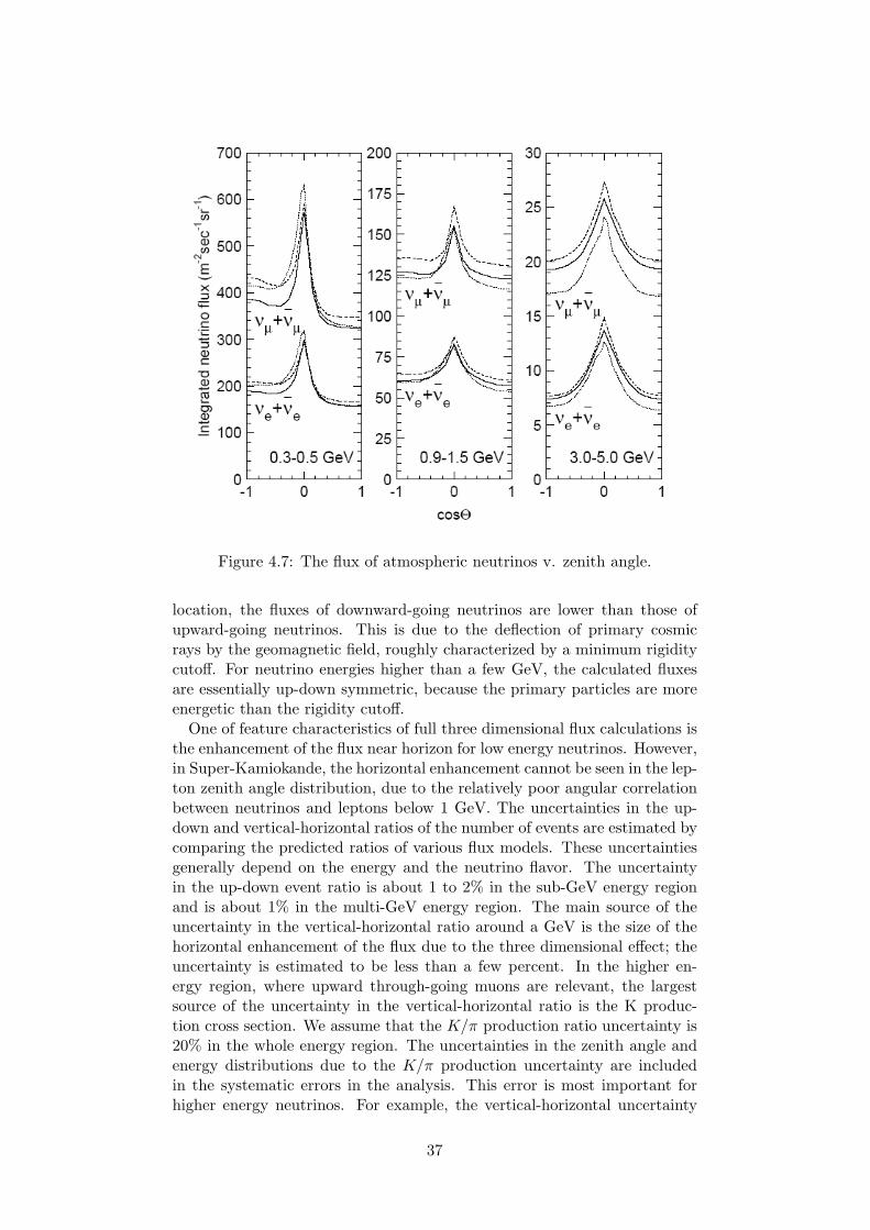
Figure 4.7: The flux of atmospheric neutrinos v. zenith angle.

location, the fluxes of downward-going neutrinos are lower than those ofupward-going neutrinos. This is due to the deflection of primary cosmicrays by the geomagnetic field, roughly characterized by a minimum rigiditycutoff. For neutrino energies higher than a few GeV, the calculated fluxesare essentially up-down symmetric, because the primary particles are moreenergetic than the rigidity cutoff.

One of feature characteristics of full three dimensional flux calculations isthe enhancement of the flux near horizon for low energy neutrinos. However,in Super-Kamiokande, the horizontal enhancement cannot be seen in the lep-ton zenith angle distribution, due to the relatively poor angular correlationbetween neutrinos and leptons below 1 GeV. The uncertainties in the up-down and vertical-horizontal ratios of the number of events are estimated bycomparing the predicted ratios of various flux models. These uncertaintiesgenerally depend on the energy and the neutrino flavor. The uncertaintyin the up-down event ratio is about 1 to 2% in the sub-GeV energy regionand is about 1% in the multi-GeV energy region. The main source of theuncertainty in the vertical-horizontal ratio around a GeV is the size of thehorizontal enhancement of the flux due to the three dimensional effect; theuncertainty is estimated to be less than a few percent. In the higher en-ergy region, where upward through-going muons are relevant, the largestsource of the uncertainty in the vertical-horizontal ratio is the K produc-tion cross section. We assume that the K/π production ratio uncertainty is20% in the whole energy region. The uncertainties in the zenith angle andenergy distributions due to the K/π production uncertainty are includedin the systematic errors in the analysis. This error is most important forhigher energy neutrinos. For example, the vertical-horizontal uncertainty

37

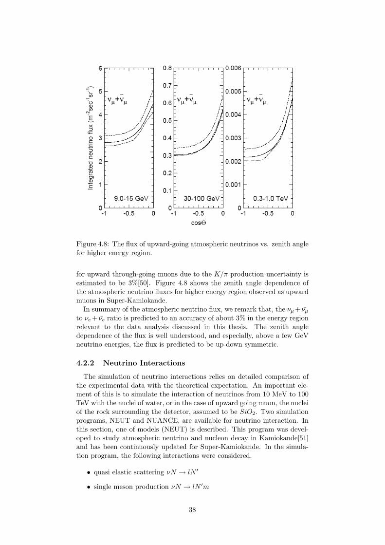
Figure 4.8: The flux of upward-going atmospheric neutrinos vs. zenith anglefor higher energy region.

for upward through-going muons due to the K/π production uncertainty isestimated to be 3%[50]. Figure 4.8 shows the zenith angle dependence ofthe atmospheric neutrino fluxes for higher energy region observed as upwardmuons in Super-Kamiokande.

In summary of the atmospheric neutrino flux, we remark that, the νµ + νµ

to νe + νe ratio is predicted to an accuracy of about 3% in the energy regionrelevant to the data analysis discussed in this thesis. The zenith angledependence of the flux is well understood, and especially, above a few GeVneutrino energies, the flux is predicted to be up-down symmetric.

4.2.2 Neutrino Interactions

The simulation of neutrino interactions relies on detailed comparison ofthe experimental data with the theoretical expectation. An important ele-ment of this is to simulate the interaction of neutrinos from 10 MeV to 100TeV with the nuclei of water, or in the case of upward going muon, the nucleiof the rock surrounding the detector, assumed to be SiO2. Two simulationprograms, NEUT and NUANCE, are available for neutrino interaction. Inthis section, one of models (NEUT) is described. This program was devel-oped to study atmospheric neutrino and nucleon decay in Kamiokande[51]and has been continuously updated for Super-Kamiokande. In the simula-tion program, the following interactions were considered.

• quasi elastic scattering νN → lN ′

• single meson production νN → lN ′m

38

• coherent π production ν16O → lπ16O

• deep inelastic scattering νN → lN ′hardron

Where, N and N ′ are the nucleons, l is the lepton, and m is the meson,respectively.

Elastic and Quasi-Elastic Scattering

The cross section of quasi-elastic scattering off a free proton, which wasused in the simulation programs, was described by Llewellyn-Smith[52]. Forthe ν16O scattering, the Fermi motion of the nucleons and Pauli ExclusionPrinciple are taken into account. The nucleons are treated as quasi-free par-ticles using the relativistic Fermi gas model of Smith and Moniz[53]. Themomentum distribution of the nucleons were assumed to be flat up to thefixed Fermi surface momentum of 225 MeV/c. This Fermi momentum dis-tribution was also used for other nuclear interactions. The nuclear potentialwas set to 27 MeV/c.

Single Meson Production

To simulate the resonance productions of single π, K and η, Rein and Se-hgal’s model[54][55] was adopted. In this model, the interaction is separatedinto two parts as follows.

νN → lN∗

N∗ → mN ′

where m is a meson, N and N ′ are nucleons, and N* is a baryon resonance.To obtain the cross sections, we calculate the amplitude of each resonanceproduction and then multiply the probability of decay into one pion andnucleon to each resonance. In order to avoid double counting of interaction,the hadronic invariant mass, W (the mass of the intermediate baryon reso-nance), is restricted to be less than 2 GeV/c2. In addition to the dominantsingle π production, K and η production is considered. To determine theangular distribution of pions in the final state, Rein and Sehgal’s method forthe P33(1232) resonance were used. For the other resonances, the directionaldistribution of the generated pions is set to be isotropic in the Adler Frame(resonance rest frame). The angular distribution of π+ has been measuredfor νp → µ−pπ+ mode[56] and the results agree well with the Monte Carloprediction. The Pauli blocking effect in the decay of the baryon resonancewas considered by requiring that the momentum of nucleon should be largerthan the Fermi surface momentum. Pion-less delta decay is also considered,where 20 % of the events do not have the pion and only the lepton andnucleon are generated[57].

There is a parameter that should be determined by experiment in thequasi-elastic scattering and single meson production. The parameter iscalled axial vector mass, MA. For larger MA values, interactions with higherQ2 values (and therefore larger scattering angles) are enhanced for thesechannels. The MA value was tuned using the K2K[58] near detector data.In our atmospheric neutrino interaction Monte Carlo simulation, MA was

39

set to 1.1 GeV for both the quasi-elastic and single meson production chan-nels, but the uncertainty of the value is estimated to be 10%. Coherentsingle pion production, the interaction between the neutrino and the entireoxygen nucleus, was simulated using the formalism developed by Rein andSehgal[59].

Deep Inelastic Scattering

The cross sections of deep inelastic scattering was calculated using theGRV94[60] for the nucleon structure function. In the calculation, the hadronicinvariant mass, W , is required to be greater than 1.3 GeV/c2. And for ac-tual calculation, we use the probability function of pion multiplicity, whichis a function of W region (W ≤ 2GeV/c2). The multiplicity of pions is re-stricted to be greater than or equal to 2 for 1.3 < W < 2.0GeV/c2, becausesingle pion production is separately simulated as previously described. Inorder to generate events with multi-hadron final states, two models wereused. For W between 1.3 and 2.0 GeV/c2, a custom made program[61] wasused to generate the final state hadrons; only pions are considered in thiscase. For W larger than 2 GeV/c2, PYTHIA/JETSET[62] was used. To-tal charged current cross sections including quasi-elastic scattering, singlemeson productions and deep inelastic scattering are shown in Figure 4.9.

Nuclear Effect

The interactions of mesons and nucleons, which are generated in 16Onucleus, are also important for the atmospheric neutrino interaction andnucleon decay. This process is simulated by a subroutine named ”eftrace”.In Chapter 6, this program is tested for systematic uncertainty of nuclearpropagation in n − n search. Basically, all of the interactions were treatedby using a cascade model. The interactions of pions are very important be-cause the cross section for pion production is quite large for neutrino energiesabove 1 GeV and the interaction cross sections for pions in nuclear matteris also large. In the simulation of pion interactions in 16O, inelastic scat-tering, charge exchange and absorption were considered. The procedure tosimulate these interactions is as follows. The initial position of the pion wasgenerated according to the Woods-Saxon nucleon density distribution[63].The interaction mode is determined from the calculated mean free path ofeach interaction. To calculate the mean free path, the model described byOset et al.[64] was adopted. The calculated mean free path depends notonly on the momentum of pion but also on the position of the pion in thenucleus. If inelastic scattering or charge exchange occurs, the direction andmomentum of the pion are determined by using the results of a phase shiftanalysis obtained from π −N scattering experiments[65]. In calculation ofthe pion scattering amplitude, the Pauli blocking effect is also taken intoaccount by requiring the nucleon momentum after interaction to be largerthan the Fermi surface momentum (PF (r)) at the interaction point definedas follows.

PF (r) = [32π2ρ(r)]−

13 (4.1)

40

Figure 4.9: Charged current total cross section divided by Eν for (a) neutrinoand (b) anti-neutrino nucleon charged current interactions. Solid line showsthe calculated total cross section. The dashed, dot and dash-dotted linesshow the calculated quasi-elastic, single-meson and deep-inelastic scattering,respectively.

41

Figure 4.10: The cross section of π16O interactions. The lines show theresults of our calculation based on [64] and the points show experimentaldata[66].

ρ(r) =Z

Aρ

1

1 + exp( |r|−ca )

(4.2)

where A(=16) is mass number, Z(=8) is atomic number, ρ(=0.48 m3π) is

average density of nucleus, a(=0.41 fm) and c(=2.69 fm) are density pa-rameters of oxygen nucleus, respectively. The pion interaction simulationwas checked using data for the following three interactions: π12C scattering,π16O scattering and pion photo-production(γ +12 C → π−+ X)[66]. One ofcomparison is shown in Figure 4.10.

4.3 Detector Simulation

The particles left the oxygen nucleus after anti-neutron annihilation orneutrino interactions are fed into a detector simulation code. The simula-tion program includes the tracks of particles, Cherenkov radiation, propa-gation of Cherenkov photons in water and the response of PMTs and thereadout electronics. The detector simulator program has been developedbased on GEANT package[67]. The program simulates the tracks of parti-cles, Cherenkov radiation, propagation of Cherenkov photons in water, andthe response of PMTs and the readout electronics. And various processesfor each particles are considered in our simulation program as listed in Table4.3.

When a π0 escapes from the oxygen nucleus or a π0 is generated by freeproton interaction, it immediately decays to two gammas (98.8% branchingratio). However, since π± has relatively long lifetime, the propagation ofπ± in water should be simulated. CALOR package[68] is employed in oursimulation code. This package is known to reproduce the pion interactions

42

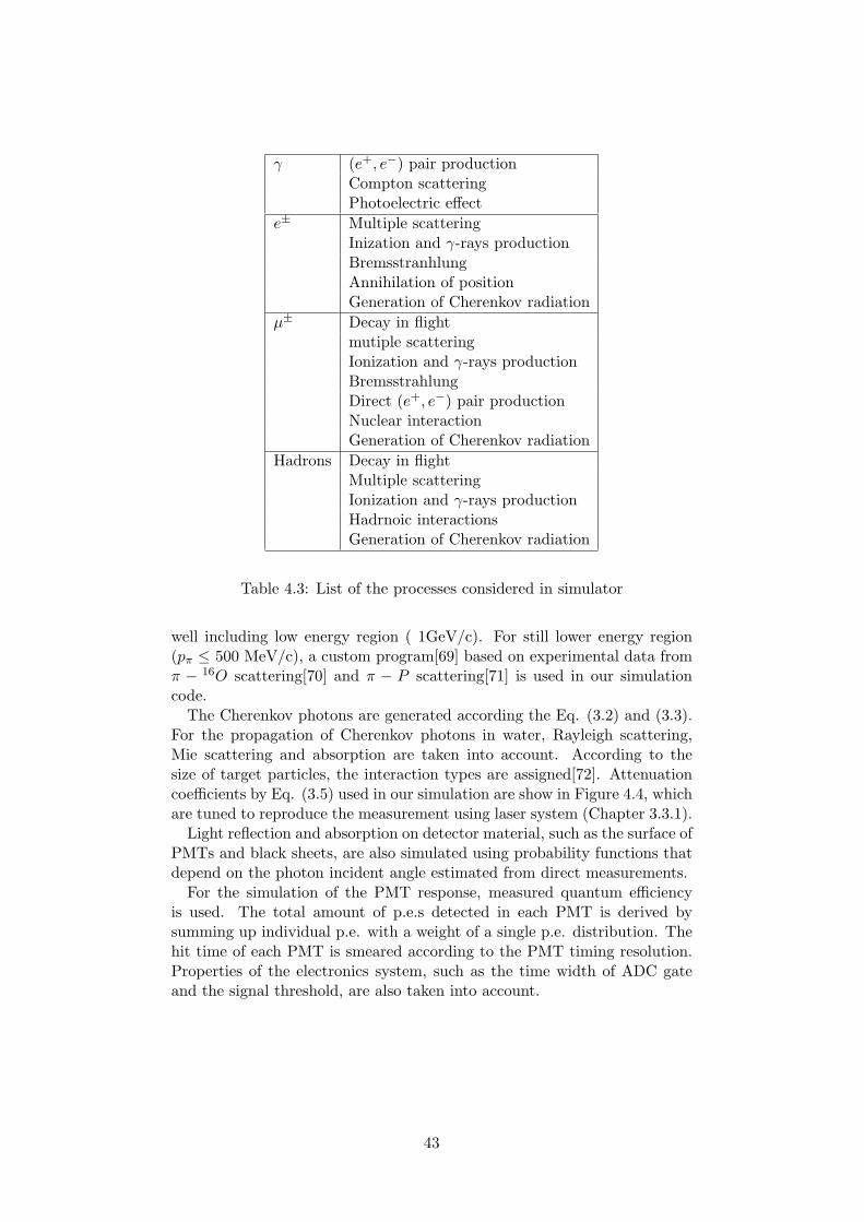
γ (e+, e−) pair productionCompton scatteringPhotoelectric effect

e± Multiple scatteringInization and γ-rays productionBremsstranhlungAnnihilation of positionGeneration of Cherenkov radiation

µ± Decay in flightmutiple scatteringIonization and γ-rays productionBremsstrahlungDirect (e+, e−) pair productionNuclear interactionGeneration of Cherenkov radiation

Hadrons Decay in flightMultiple scatteringIonization and γ-rays productionHadrnoic interactionsGeneration of Cherenkov radiation

Table 4.3: List of the processes considered in simulator

well including low energy region ( 1GeV/c). For still lower energy region(pπ ≤ 500 MeV/c), a custom program[69] based on experimental data fromπ − 16O scattering[70] and π − P scattering[71] is used in our simulationcode.

The Cherenkov photons are generated according the Eq. (3.2) and (3.3).For the propagation of Cherenkov photons in water, Rayleigh scattering,Mie scattering and absorption are taken into account. According to thesize of target particles, the interaction types are assigned[72]. Attenuationcoefficients by Eq. (3.5) used in our simulation are show in Figure 4.4, whichare tuned to reproduce the measurement using laser system (Chapter 3.3.1).

Light reflection and absorption on detector material, such as the surface ofPMTs and black sheets, are also simulated using probability functions thatdepend on the photon incident angle estimated from direct measurements.

For the simulation of the PMT response, measured quantum efficiencyis used. The total amount of p.e.s detected in each PMT is derived bysumming up individual p.e. with a weight of a single p.e. distribution. Thehit time of each PMT is smeared according to the PMT timing resolution.Properties of the electronics system, such as the time width of ADC gateand the signal threshold, are also taken into account.

43

Figure 4.11: Wavelength dependence of attenuation coefficient (L−1attenu) ob-

tained by light scattering measurement. Point is measurement in Chapter3.3.1.

44

Chapter 5

Data Reduction andReconstruction:Fully-Contained Events

The Super-Kamiokande I data was acquired from May, 1996 to July, 2001.The data are classified into three groups; fully-contained (FC), partially-contained (PC) and upward-going muons (UPMU). To separate FC and PCevents, a fast spatial clustering algorithm is applied to the outer detectorhits; if the number of hits in the largest OD cluster is less than 10, the eventsis defined as fully-contained. Otherwise, it is defined as partially-contained.The neutrino energies of partially-contained events are typically 10 timeshigher than that of fully-contained. Figure 5.1 shows the separation.

The analyses using these two data sets are based on independent datareduction and reconstruction. This section outlines the programs for reduc-tion and reconstruction for fully-contained data which is used in atmosphericneutrino and nucleon decay (including n − n search) analysis. These sameprograms are also applied to atmospheric neutrino MC and n− n MC.

5.1 Data Reduction

The Super-Kamiokande has been taking the data with the trigger rateof 10 Hz every day except for 10% down time due to detector calibration,maintenance of detector and so on. 2.7 Hz are due to cosmic ray muonand 6 Hz are due to relatively low energy (a few MeV) events caused byradioactivity in the detector water or gamma rays from surrounding PMTsand rocks. Remaining 1 Hz are due to fake triggers caused by reflection ofPMT signals and unwanted PMT signals following highly energetic events(so-called ”after pulsing”). Therefore, we should eliminate these backgroundto find the possible n − n events from the cosmic ray events. Cosmic raymuons are easily discriminated by requiring little or no ring activity in theouter detector. For atmospheric neutrino and nucleon decay analysis, weconsider the events with visible energy above 30 MeV where visible energy(Evis) is defined as the energy of an electromagnetic shower that gives acertain amount of Cherenkov light (for example, a muon of momentum 300MeV/c yields a visible energy of about 110 MeV). To make the final FC

45

Figure 5.1: The number of hits in the largest outer detector cluster, which isused to separate the fully-contained and partially-contained event samples.The histogram shows the MC prediction with neutrino oscillation.

data sample, the following five steps of data reduction criteria are used.

5.1.1 1st and 2nd Reduction

Simple and efficient criteria are applied in the first and second reductionsteps:

• PE300 > 200 p.eWhere, PE300 is the maximum total photo electrons collected in theinner detector within a 300 nsec sliding time window.

• PEmax/PE300 < 0.5Where, PEmax is the maximum p.e. in any single ID PMT.

• NHITA800 < 25 hitsWhere, NHITA800 is the number of hit OD PMT within 800 nsecsliding time window.

• TDIFF > 100µ secWhere TDIFF is the time interval from the preceding event. This isto reject electrons from stopping muon decays.

5.1.2 Third Reduction

More complex criteria are applied in the third reductions step for furtherrejection of cosmic ray muons and low energy events:

• NHITAin < 10 hits and NHITAout < 10 hitsWhere, NHITAin (NHITAout) is the number of hit OD PMTs within

46

8 m from the entrance (exit) point of muon track fitted using the innerdetector light pattern.

• NHIT50 ≥ 50 hitsWhere, NHIT50 is the number of hit ID PMTs in 50 nsec sliding timewindow.

5.1.3 Fourth Reduction

Additional selection criteria are used to eliminate spurious events, suchas ”flashing” PMTs that emit light from internal corona discharges. Flasherevents are removed by two different methods.

• Typical flasher events have broader PMT timing distributions thanthe neutrino events. Events with broader timing distributions areeliminated.

• Since flasher events have a tendency to be repeated with similar spatialhit distribution, the pattern information of observed charge is used onto eliminate these events. A correlation parameter based on the chargepattern is calculated with other data events and a ”matched” tag isassigned for highly correlated events.

A cut is applied based on maximum correlation value and the number of”matched” with other events.

5.1.4 Fifth Reduction

Two further event types are eliminated in the fifth reduction step.

• NHITAoff < 10 hitsWhere NHITAoff is the number of OD hits in 200 nsec sliding timewindow preceding the trigger time (-8900 ∼ -100 nsec). This cut elim-inates decay electrons from invisible cosmic ray muons that are belowCherenkov threshold in the inner detector.

• Cosmic ray muons are removed using a more precise fitter and thesame criteria as the first cut of (3).

Finally, the vertex is required to be within a fiducial volume (FV), 2 metersfrom the wall of the inner detector, and the visible energy is required to begreater than 30 MeV. Table 5.1 shows the event rate after each reductionstep.

5.2 Reconstruction

The fully-contained events after passing through the data reduction, un-dergo reconstruction process.

47

Reduction step Data Monte CarloTrigger 1,889,599,293 14,013.9 (100.00%)First reduction 4,591,695 14,006.3 (99.95%)Second reduction 301,791 14,006.1 (99.94%)Third reduction 66,810 13,993.3 (99.85%)Fourth reduction 26,937 13,898.1 (99.17%)Fifth reduction 23,984 13,895.3 (97.15%)FV and Evis cuts 12,180 13,676.7 (97.59%)

Table 5.1: Number of events after each reduction for fully-contained eventsduring 1489 days of the detector live-time. The Monte Carlo numbers andefficiencies down to the fifth reduction are for events whose real vertex is inthe fiducial volume, the number of outer detector hits fewer than 10 and thevisible energy larger than 30 MeV. In the last line, the fitted vertex is usedfor both data and Monte Calro.

5.2.1 Vertex Fitting

The reconstruction process starts from vertex fitting. The vertex fittingconsists of following three steps.

1. Point-fit : The point at which the timing residual distribution of hitPMTs has the sharpest peak is estimated.

2. Ring edge search : The direction and outer edge of the dominant ringis estimated by the Cherenkov opening angle expected from the chargewithin the cone.

3. TDC-fit : the track length of the charged particle and scattered Cherenkovphotons are taken into account in the calculation of the time residual.

The vertex resolution is estimated to be 30 cm for single-ring fully-containedevents. The vertex positions are more precisely estimated later by MS-fitusing ring pattern.

5.2.2 Ring Counting

After a ring direction and vertex are roughly found through the previousvertex fitting algorithm, other possible rings are searched using a Houghtransform[73] based technique. The technique is iterative. A second ring issearched for by choosing possible ring directions based on the Hough map,and a likelihood technique determined if a second ring from the list of thepossible rings is more consistent with the data than just one ring. If a secondring is judged to be more consistent, then this procedure is repeated asmany as necessary until finally no further rings are necessary to fit the data.Figure 5.2 shows the likelihood difference between the 2 ring assumptionand a 1 ring assumption. In these figures, the oscillation at the best fitparameters (sin22θ = 1.0, ∆m2 = 2.1 × 10−3eV 2) was taken into accountfor the Monte Carlo prediction. A cut was made at likelihood difference

48

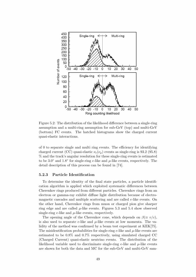
Figure 5.2: The distribution of the likelihood difference between a single-ringassumption and a multi-ring assumption for sub-GeV (top) and multi-GeV(bottom) FC events. The hatched histograms show the charged currentquasi-elastic interactions.

of 0 to separate single and multi ring events. The efficiency for identifyingcharged current (CC) quasi-elastic νe(νµ) events as single-ring is 93.2 (95.8)% and the track’s angular resolution for these single-ring events is estimatedto be 3.0◦ and 1.8◦ for single-ring e-like and µ-like events, respectively. Thedetail description of this process can be found in [74].

5.2.3 Particle Identification

To determine the identity of the final state particles, a particle identifi-cation algorithm is applied which exploited systematic differences betweenCherenkov rings produced from different particles. Cherenkov rings from anelectron or gamma-ray exhibit diffuse light distribution because of electro-magnetic cascades and multiple scattering and are called e-like events. Onthe other hand, Cherenkov rings from muon or charged pion give sharperring edge and are called µ-like events. Figures 5.3 and 5.4 show observedsingle-ring e-like and µ-like events, respectively.

The opening angle of the Cherenkov cone, which depends on β(≡ v/c),is also used to separate e-like and µ-like events at low momenta. The va-lidity of the method was confirmed by a beam test experiment at KEK[75].The misidentification probabilities for single-ring e-like and µ-like events areestimated to be 0.8% and 0.7% respectively, using simulated charged CC(Charged Current) quasi-elastic neutrino events. The distribution of thelikelihood variable used to discriminate single-ring e-like and µ-like eventsare shown for both the data and MC for the sub-GeV and multi-GeV sam-

49

Figure 5.3: An event display of a single-ring e-like.

Figure 5.4: An event display of a single-ring µ-like.

50

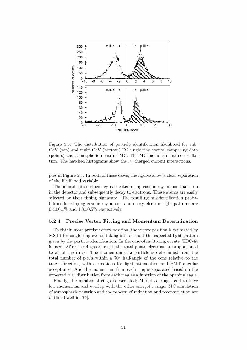
Figure 5.5: The distribution of particle identification likelihood for sub-GeV (top) and multi-GeV (bottom) FC single-ring events, comparing data(points) and atmospheric neutrino MC. The MC includes neutrino oscilla-tion. The hatched histograms show the νµ charged current interactions.

ples in Figure 5.5. In both of these cases, the figures show a clear separationof the likelihood variable.

The identification efficiency is checked using cosmic ray muons that stopin the detector and subsequently decay to electrons. These events are easilyselected by their timing signature. The resulting misidentification proba-bilities for stoping cosmic ray muons and decay electron light patterns are0.4±0.1% and 1.8±0.5% respectively.

5.2.4 Precise Vertex Fitting and Momentum Determination

To obtain more precise vertex position, the vertex position is estimated byMS-fit for single-ring events taking into account the expected light patterngiven by the particle identification. In the case of multi-ring events, TDC-fitis used. After the rings are re-fit, the total photo-electrons are apportionedto all of the rings. The momentum of a particle is determined from thetotal number of p.e.’s within a 70◦ half-angle of the cone relative to thetrack direction, with corrections for light attenuation and PMT angularacceptance. And the momentum from each ring is separated based on theexpected p.e. distribution from each ring as a function of the opening angle.

Finally, the number of rings is corrected; Missfitted rings tend to havelow momentum and overlap with the other energetic rings. MC simulationof atmospheric neutrino and the process of reduction and reconstruction areoutlined well in [76].

51

Chapter 6

Search for n− n Oscillation

We should extract the candidates of n − n oscillation from the Super-KI data set of 24.5×1033 neutron-yr. For this work, additional criteria areapplied to the remaining fully-contained (FC) data after passing throughthe reduction algorithm. Studying the FC atmospheric neutrino MC as amost significant source of background, we can estimate the upper limit ofthe number of n − n oscillation signal. Finally, the lower limit on neutronoscillation time is calculated with inclusion of systematic errors. In thisthesis, 5,000 n − n events inside of fiducial volume (FV) and 100 years FCatmospheric neutrino MC are simulated for Super-K I data set.

6.1 Event Selection Criteria

Candidates of n − n oscillation are extracted based on (a) Number ofrings, (b) Visible energy, (c) Total momentum and (d) Total invariant mass.The number of rings are understood particles produced by the interactionand visible energy is defined as the energy of an electromagnetic showerthat gives a certain amount of Cherenkov light. The total momentum isdefined as Ptot = |∑allrings

i−→pi | where −→pi is reconstructed momentum vector

of i-th ring and the total invariant mass is defined as Mtot =√

E2tot − P 2

tot

where total energy Etot =∑allrings

i |−→Pi|. Figure 6.1 is comparison of above4 variables among the n− n MC, atmospheric neutrino MC and data afterreduction and reconstruction processes in same way. To compare the plots,one addition is taken into account. Strong evidence has been presented thata νµ can oscillate to either a ντ or a sterile ν and this effect is observed onlyin charged current interaction. Therefore in the case of atmospheric neutrinoMC, oscillation effect is applied at the sin22θ = 1 and ∆m2 = 0.0021 as Eq.(6.1) since MC was made without considering the oscillation. As the plotsshow, the number of rings and visible energy are efficient variables to selectthe candidates. So, we can make first criterion to reject dominant back-ground which comes from single ring events. The criterion rejects around64% background events. Figure 6.2 is the visible energy distribution afterrejecting the single ring events.

P (νµ → νµ) = 1− sin22θsin2(1.27∆m2L

Eν) (6.1)

52

Our goal is to find the n− n oscillation events and calculate the oscillationtime. If we don’t find the events, we set the lower limit of oscillation time.The lifetime for neutron oscillations is estimated by

Tn−n =ε×N × T

S. (6.2)

• ε : signal detection efficiency

• N : number of neutrons inside of fiducial volume

• T : detector livetime

• S : the upper limit on mean of number of signal at 90% CL

and the procedure of calculation is described in Chapter 6.3.For optimization of selection criteria, signal significance is considered

based on above calculation as follows ;

s√b

=ε×N × T × Γ√

b(6.3)

where Γ is event rate and b is number of background candidates. SinceN × T × Γ is consistent,

s√b∝ ε√

b(6.4)

ε/√

b is used as a factor for criteria optimization. Optimal cut is foundscanning the region which is low momentum and high invariant mass basedon maximum value of ε/

√b ;

(a) Number of rings > 1(b) 700MeV < Visible energy < 1300MeV(c) 0 MeV/c < Total momentum < 450MeV/c(d) 750MeV/c2 < Total invariant mass < 1800MeV/c2

Criterion (a) and (b) rejected the 94% background events and saved 33.5%n−n MC and 6% signal. Figure 6.3 shows the total momentum and invariantmass distribution after passing through the criterion (a) and (b). Additionalkinematical cuts, (c) and (d) made final sample which is inside of arrows infigure 6.4 for analysis.

6.2 Background

As mentioned above, the most significant source of background in n − nsearch comes from the atmospheric neutrino interactions as which on anaverage 8 FC events are detected per day during Super-K I full livetime.Therefore, investigation of the n− n mimic events is performed using the FCatmospheric neutrino MC. 521 FC atmospheric neutrino simulation eventswithout inclusion of oscillation effect are alive after passing through theevent selection criteria which was mentioned in previous section. The char-acteristic is listed up in Table 6.1 in detail. Electron neutrino and muonneutrino have almost same contribution to background but muon neutrinowill be decreased by neutrino oscillation. And anti neutrino events are much

53

Figure 6.1: Basic plot comparisons : Each plot show Number of rings(Nring), Visible energy (Evis), Total momentum (Ptot) and Total invari-ant mass (Mtot). Vertical axes are normalized by the number of events andoscillation effect was applied in the case of atmospheric neutrino MC. Apeak between 100 and 200MeV/c2 of Mtot distribution is caused by π0.

54

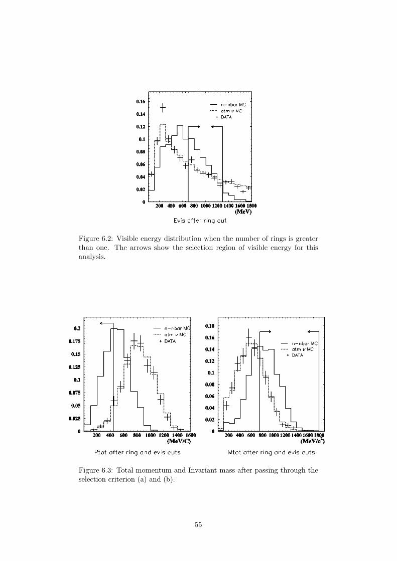
Figure 6.2: Visible energy distribution when the number of rings is greaterthan one. The arrows show the selection region of visible energy for thisanalysis.

Figure 6.3: Total momentum and Invariant mass after passing through theselection criterion (a) and (b).

55

Figure 6.4: Invariant mass after passing through the selection criterion (a),(b) and (c).

less than neutrino events. Main contribution is single pion and multi pionproduction. The reason can be simply understood, produced pions and par-ticles by neutrino interaction and secondaries make multi rings. Remark-able thing is, topologically even though charged current quasi elastic eventsshould be separated from n − n events since they have lager momentum,they survived in analysis sample because energetic outgoing nucleon madehadron interactions. The neutral current elastic events are also survived insame way. Figure 6.5 shows the parent neutrino energy distribution for allof background events.

6.3 Results

Final detection efficiency of n − n events and the number of backgroundand candidates after passing through above criteria are summarized in Table

νµ νµ νe νe

CC quasi elastic 11 (2.11%) 0 7 (1.34%) 0CC single π prod. 50 (9.6%) 10 (1.92%) 47 (9.02%) 7 (1.34%)CC multi π prod. 101 (19.38%) 10 (1.92%) 103 (19.77%) 9 (1.73%)CC K or η prod. 6 (1.15%) 6 (1.15%) 8 (1.53%) 1 (0.19%)NC single π prod. 17 (3.26%)NC multi π prod. 125 (23.99%)NC K or η prod. 2 (0.38%)NC elastic 1 (0.19%)

Table 6.1: List of background events.

56

Figure 6.5: Parent neutrino energy of background events. Left figure showsabout 521 background events in total and right figure shows in each inter-action mode.

6.2. For this estimation, atmospheric neutrino MC considered the oscillationeffect and overall normalization[76], a factor of 1.119, and is normalized bylivetime. The detection efficiency is 10.4% and the candidates from Super-K I of 91.7kton-year exposure are 20 events in which 21 background eventsare allowed. Figure 6.6 shows final sample for analysis which is selected bykinematical cuts.

6.3.1 Simple Limit Calculation

When we observe N particles for a time T and find a nonzero number ofevents, n, with the detection efficiency, ε, the event rate, Γ is estimated by;

Γ =n

NTε(6.5)

However, when n is zero, a rate can not be accurately calculated and n is nolonger a good estimator of the true mean. So, instead, a limit on the eventrate (oscillation rate in this thesis) at some confidence level is set.

Our result has 20 candidate events but also has background with almostsame level. So, we interpret our result as lower limit of n − n oscillation

Criterion n → n MC (%) atm. ν MC (%) DATA (%)Inside of F.V. 5000 13028.9 12180Nring cut 4275 (85.5) 4676.7 (35.8) 3865 (31.7)Evis cut 1673 (33.5) 909.5 (7.0) 731 (6.0)Ptot and Mtot cut 521 (10.4) 21.6 (0.16) 20 (0.16)

Table 6.2: Number of events and detection efficiency after each criterion.

57

Figure 6.6: Total invariant mass versus total momentum. The events insideof right lower box in each scatter plot are final sample selected by kinematicalcuts for n− n oscillation analysis. With 10.4% detection efficiency in which521 events are detected among 5,000 n − n events, 20 candidates and 21background events are observed.

58

time and the limit is calculated by Eq. (6.2) using the quantities in Table6.2. In simple case, it is common to use the method of Poisson Process withBackground[77]. However since this method does not take any uncertaintiesthat we may have in the parameters to get the limit, the final limit will beestimated with other method considering the effect of systematic errors inlast of this Chapter. Firstly, assuming that the systematic uncertainty isnegligible and the number of background(µB) is known, the lower limit ofoscillation time is calculated simply.

The upper limit on mean of the number of signal S in Eq. (6.2) can bedefined using Poisson distribution[77]:

CL = 1− e−µB+S ∑n0n=0

(µB+S)n

n!

e−µB∑n0

n=0(µB)n

n!

(6.6)

where CL is a confidence level and n0 is the number of observed candidates.Applying n0 = 20 and µB = 21.6, the upper limit S is calculated to be 7.95at the 90% confidence level. Based on this S, the lower limit on the neutronoscillation time is calculated as:

Tn−n =ε× v ×NA × 8neutrons

18g × T

S(6.7)

For exposure, v is the fiducial volume of 22.5 kton, NA is Avogadro’s num-ber and T is livetime of 4.07 years. ε is the efficiency to detect neutronoscillations, 10.4%. Therefore, the neutron oscillation time limit is calcu-lated to be 3.2×1032 yr at the 90% confidence level for 24.5×1033 neutron-yr.

6.3.2 Limit for Free Neutrons

The lifetime of a neutron bound in a nucleus with A nucleons (TA) is muchlarger than that of a free neutron (τfree) due to the suppression of neutronoscillations by a potential barrier at the edge of the nuclear potential well.

As already mentioned, our search in this thesis is about intranuclear pro-cess. Limit can be converted to the limit for free neutron by theoreticalnuclear suppression factor[12][13][14] with following relation.

T (intranuclear) = R · τ2nn(free) (6.8)

where R is dimensional ”suppression factor” equal to ∼ 2 · 1023sec−1 for themost of nuclei. This can be understood from the following considerationssimply.

The neutron bound in nucleus by energy ∆E(∼ 10MeV ) is quasi-free forthe time

∆t ∼ 1∆E

∼ 10−22sec (6.9)

Probability of n− n oscillation during the time ∆t is

P = (∆t

τnn)2 (6.10)

59

and above condition occurs per second.

P =1

T (intranuclear)= (

∆t

τnn)2

1∆t

=∆t

(τnn)2(6.11)

Intranuclear process are heavily suppressed by R.

T (intranuclear) = R · (τnn(free))2 (6.12)

R ∼ 1∆t

∼ 1022s−1 (6.13)

We call R as nuclear suppression factor. Theoretical progresses on R aredescribed on [12][13][14] and R of 16O is suggested (0.46 ∼ 1.93) × 10−23

by Dover et al., (1.7 ∼ 2.6)× 10−23 by Alberico and (0.6 ∼ 3.6)× 10−23 byHufner and Kopeliovich. The most conservative limit is R = 3.6 × 1023s−1

in most recent theoretical treatment of [14].Finally, oscillation time limit on bound neutron in previous section can

be translated to 1.67 × 108s on free neutron by most conservative limit ofnuclear suppression factor.

6.4 Systematic Errors

We simulated n− n oscillation and background for n− n search and gotthe lower limit on neutron oscillation time. However, the limit is affectedby uncertainties in detection efficiency and background due to imperfectionof simulation and measurement. In this section, I estimate the systematicerrors in our n− n analysis.

6.4.1 Uncertainties in Efficiency and Exposure

Incompleteness and model dependence in simulation of n − n oscillationlead to systematic errors. By estimating the contribution to detection effi-ciency and exposure from each source of uncertainties, systematic errors inanalysis are obtained. The sources of uncertainties are listed up below;

• Detection efficiency

– Fermi momentum

– Annihilation branching ratio

– Nuclear effect

– Un-uniformity of detector gain

– Energy scale

– Ring counting

• Exposure

– Detector livetime

– Fiducial volume

60

Figure 6.7: Fermi momentum distribution.

The uncertainty is caused by imperfect knowledge of n − n oscillationkinematics. First, I estimated how much fermi momentums of anti-neutronand nucleon, which participate in annihilation process, affect to detectionefficiency. Figure 6.7 shows fermi momentum of anti-neutron which wastransited from neutron. Changing the fermi momentum by 20%, the con-tribution to detection efficiency is estimated to be 4.2%. And annihilationbranching ratio can be source of uncertainty. Table 4.1 and 4.2 in Chapter4 show the annihilation branching ratios which are used in this thesis andother experiments. For uncertainty estimation, we generated n − n oscilla-tion MC with other branching ratios, Baltay(1966) for n − n annihilationand Bettini(1967) for n − p annihilation, and got the change of detectionefficiency by 5.2%. Nuclear effect in pionic phase after annihilation is con-sidered as a main source of uncertainty in efficiency. The errors of crosssection are taken from the figure 4.2. Increasing the probability by 20%of elastic, 30% of charge exchange, 25% of absorption and 30% π produc-tion, the uncertainty in efficiency is estimated to be 12.5%. And to checkmodel dependency of nuclear effect, nuclear propagation program ”eftrace”for nucleon decay study in Super-K analysis is called in n − n simulationprocess instead of ”partnuc” which is n − n own nuclear propagation pro-gram. Obtaining the small uncertainty of 1.7%, the reasonable consistencyof our simulation is checked with other Model.

And event selection and reconstruction process include possible sourcesof uncertainties. For ”neutrino” oscillation study[76] in Super-K, the dif-ference of energy scale between upward-going and downward-going eventswas measured using decay electrons from cosmic ray stopping muons. Theup/down asymmetry of energy scale was estimated to be 0.6% and this un-uniformity of energy scale can affect momentum measurement which is oneof criteria for n − n search. Therefore by changing the momentum cut by±1.2%, we obtained 4% uncertainty in efficiency. In neutrino oscillation

61

study in Super-K, the uncertainty of energy scale for fully-contained eventswas also estimated to be 2%. Based on this report, visible energy cut ischanged by 2.5% and the contribution to efficiency is estimated to be 1.7%.And for final consideration, we tested the possibility of uncertainty from ringcounting and I’d like to describe procedure of this study in detail below.

Ring candidates are tested by a likelihood method as explained in Chapter5.2.2. If there is systematic difference of likelihood between data and MCdue to some reason (water transparency, incomplete understanding of thegeometry etc.), it can be source of uncertainty. To investigate the systematicdifference of likelihood, atmospheric neutrino data and MC between 8,000p.e. and 13,000 p.e. are selected as the sample. Comparing the likelihooddistribution between data and MC with some offset, we find the minimum χ2

defined as (data− αMC)2/σ2. Figure 6.8 shows the likelihood comparisonand χ2 result for 1ring/2more ring separation. The center values of parabolafitted around the minimum χ2 region are taken as systematic errors of like-lihood function. This process is also applied for higher ring separations andFigure 6.9 shows the results. The quantities of the errors estimated aboveare summarized in Table 6.3. Finally to estimate the uncertainty causedby ring counting in efficiency of n− n search, ring reconstruction process isnewly applied to n− n MC with new likelihood threshold changed by the er-ror estimated in each ring separation. Changing the threshold of likelihood,the number of n− n events passing through selection criteria is changed by0.6%.

Separation minimum χ2 ± 1σ

1ring/2more ring - 0.733 ±0.1372ring/3more ring - 0.623 ±0.1423ring/4more ring - 0.804 ±0.2974ring/5more ring + 0.198 ±0.480

Table 6.3: Fitted minimum χ2 of likelihood function for ring counting. Weassume these difference from same reason and change the threshold coher-ently.

Oscillation time limit is also directly affected by exposure. So, the uncer-tainties in the exposure are estimated. The livetime is calculated from the48bit clock counter information recorded in TRG module. The uncertaintyof the observed livetime is estimated by comparing the clock counter withanother clock counter to be < 0.1%. Lastly, uncertainty of fiducial volume isestimated by comparing the number of events inside and outside of fiducialvolume in the case of FC data and MC as follows ;

DATAin/DATAout

MCin/MCout= 0.99± 0.03 (6.14)

Above estimation is done using the events of which the number of ring isover two and visible energy is over 30GeV. Uncertainty of fiducial volume isestimated to be 3.2%.

62

Figure 6.8: Likelihood distribution and minimum χ2.

All of uncertainties in efficiency and exposure are summarized in Table6.4 and systematic uncertainty in total is estimated to be less than 15.2%.

Uncertainty (%)Detection Efficiency 14.9fermi momentum 4.2annihilation branching ratio 5.2un-uniformity of detector gain 4.0energy scale 1.7ring counting 0.6nuclear propagation (model dependence) 1.7nuclear propagation (cross section) 12.5Exposure < 3.2detector livetime <0.1fiducial volume 3.2Total <15.2

Table 6.4: Systematic uncertainties in efficiency and exposure.

6.4.2 Uncertainties in Background

The uncertainties in background also affect to the lower limit on n− n os-cillation time. Neutrino flux and interaction can be sources of uncertaintiessince we suppose the fully-contained atmospheric neutrino is main back-ground. And uncertainties related to events selection and reconstructionare also considered, such as un-uniformity, energy scale and ring countingin common with the estimation of uncertainty in efficiency.

The detail descriptions of the uncertainties for the atmospheric neutrinoflux and interaction in MC simulation were presented in Chapter 4.2 and 4.3.

63

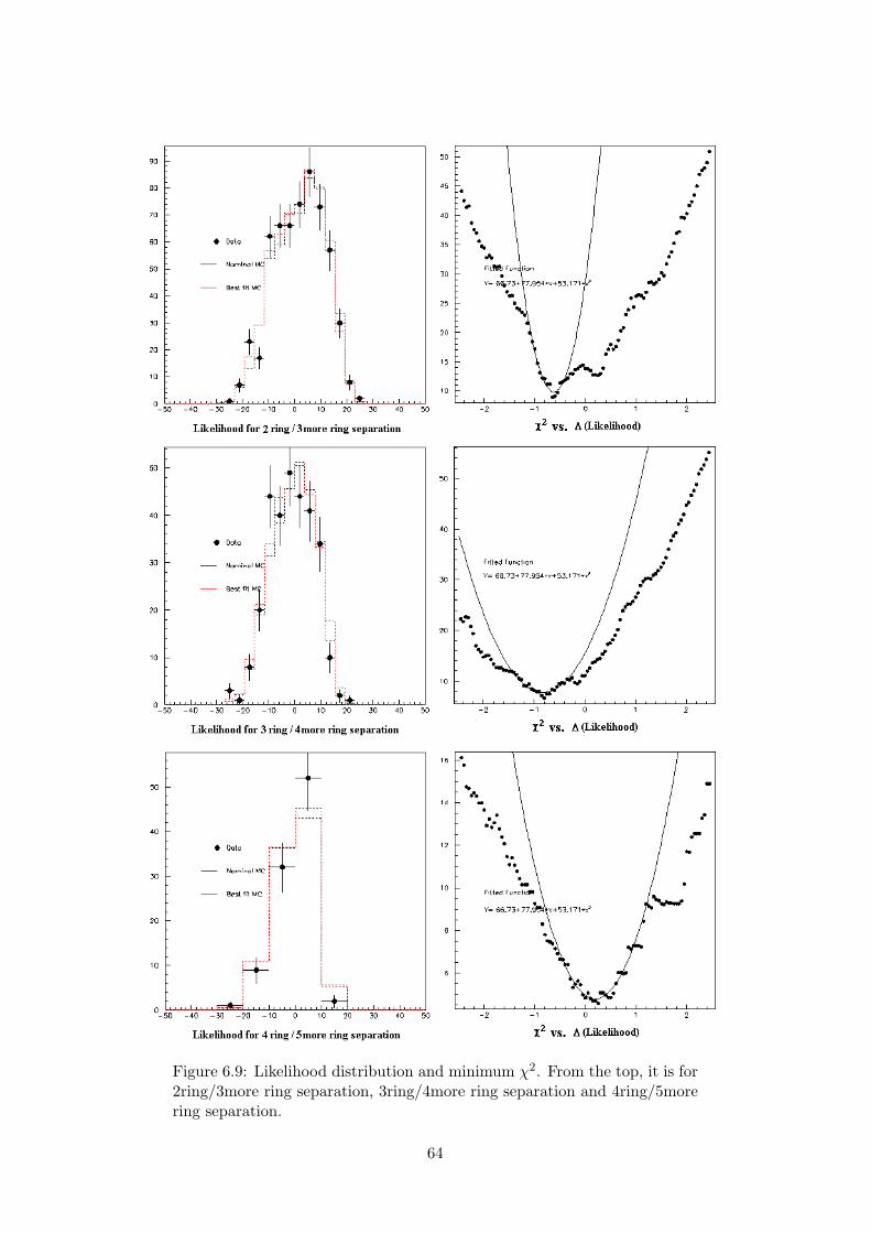
Figure 6.9: Likelihood distribution and minimum χ2. From the top, it is for2ring/3more ring separation, 3ring/4more ring separation and 4ring/5morering separation.

64

By changing the neutrino flux and interaction by the errors, uncertainties inbackground rate are estimated and summarized in Table 6.5. Uncertaintiesby un-uniformity, energy scale and ring-counting are estimated in same wayof estimation in efficiency. Changing the boundary values of selection criteriafor visible energy and total momentum changes the number of backgroundby 9% and 12% respectively. And to estimate uncertainty by ring-counting,ring reconstruction process which has the change of likelihood threshold bythe errors is applied to FC atmospheric neutrino MC and contribution tobackground rate is estimated to be 4.3%. The total systematic uncertaintyin background rate is estimated to be 32.1%.

Err.(%) Uncert.(%)Neutrino Flux 21.5flux absolute normalization 20 20flavor ratios (Eν < 5GeV, > 5GeV ) 3, 3-10, -, 0.1νe/νe ratio (Eν < 10GeV,> 10GeV ) 5, 5-10 0.9, -νµ/νµ ratio (Eν < 10GeV, > 10GeV ) 5, 5-25 0.8, -up/down ratio 0.4-2.1 -horizontal/vertical ratio 0.3-2.8(3D calc.) -K/π ratio 20 5.2energy spectrum 0.05 for 5.8

Ep > 100GeV

Neutrino Cross Section 18MA in quasi-elastic and single-π 10 4.4QE scattering (model dependence) 1σ=Fermi-gas -

vs. OsetQE scatttering (cross section) 10 0.4single-π production (cross section) 10 2.8multi-π production (model dependence) 1σ=w/ vs. 15.5

w/o Bodekmulti-π production (cross section) 5 3.4coherent π production (cross section) 30 0.1NC/CC ratio 20 6.2nuclear effect in 16O (mean free path) 30 2.7Un-uniformity of Detector Gain 9.0Energy Scale 12.0Ring Counting 4.3Total 32.1

Table 6.5: Systematic uncertainties in background rate.

65

6.5 Final Limit Calculation

In section 6.3, simple limit calculation using Poisson distribution is per-formed assuming the systematic uncertainties to be negligible. In this sec-tion, all of systematic uncertainties are included in the limit calculation byemploying a Bayesian method[78][79].

6.5.1 Description of Method

The expected mean number of candidates, µ, in our data sample is

µ = Γλε + b (6.15)

where Γ is the true event rate (n−n oscillation rate in this analysis), λ = NTis the true exposure, ε is the true efficiency to detect oscillation events andb is the true mean number of background events. In the counting exper-iments, the probability to detect n events follows the Poisson distributionwith Poisson parameter µ.

P (n|Γλεb) =e−(Γλε+b)(Γλε + b)n

n!(6.16)

P (A|B) represents the probability of proposition A, given that propositionB is true.

Applying Bayes’ theorem allows us to write

P (Γλεb|n)P (n) = P (n|Γλεb)P (Γλεb). (6.17)

Because quantities Γ, λ, ε, b are independent, P (Γλεb) can be disintegrated.

P (Γλεb) = P (Γ)P (λ)P (ε)P (b) (6.18)

The quantity in which we are interested, probability density function of Γcan be obtained by

P (Γ|n) =∫ ∫ ∫

P (Γλεb|n)dλdεdb. (6.19)

By combining above four equations, we obtain

P (Γ|n) = A

∫ ∫ ∫e−(Γλε+b)(Γλε + b)n

n!P (Γ)P (λ)P (ε)P (b)dλdεdb. (6.20)

Above normalization factor A is resolved by demanding∫ ∞

0P (Γ|n)dΓ = 1. (6.21)

P (Γ), P (λ), P (ε), P (b) in Eq. (6.20) are prior probability density functions(priors) and they enable us to include systematic uncertainties in the limitcalculation. Finally, we can calculate the upper limit of the event rate Γlimit

by

CL =∫ Γlimit

0P (Γ|n)dΓ. (6.22)

In this thesis, the limit is calculated at the 90% CL and the lifetime limit(oscillation time limit in this analysis) is the inverse of Γlimit.

66

6.5.2 Priors

There are two classes of priors in this method. One contains Γ, the othercontains ε, λ and b. In the former case, Γ is the parameter we wish toestimate with the experiment and in the latter, the parameters are notdirectly interesting and are marginalized out of the final result appearing incalculation process. Each prior is discussed below.

The prior for the event rate P (Γ) is taken to be uniform. This correspondsto the uniform prior implicitly used in simple Poisson limits[77].

P (Γ) ∝ { 1 Γ > 00 otherwise

(6.23)

The priors for the exposure P (λ) and detection efficiency P (ε) are takenas Gaussian distributions, truncated to disallow unphysical regions.

P (λ) ∝ { e−(λ−λ0)2/2σ2λ λ > 0

0 otherwise(6.24)

P (ε) ∝ { e−(ε−ε0)2/2σ2ε 0 < ε < 1

0 otherwise(6.25)

where λ0 and ε0 are estimated exposure and efficiency. The values of σλ andσε are taken from the Table 6.4 in the previous section.

The background prior P (b) is taken to be a convolution of Poisson andGaussian distributions in order to account for both the statistical uncer-tainty of a finite background MC sample size and the systematic uncertaintyin the background MC sample.

P (b) ∝∫ ∞

0

e−bMC(bMC)nb

nb!e− (bC−bMC )2

2σ2b dbMC (6.26)

where

• nb: MC events passing through n− n oscillation criteria.

• bMC : true mean MC events passing through n− n oscillation criteria.

• C: MC oversampling factor.

• σb: uncertainty due to neutrino fluxed and cross sections etc.

6.5.3 Results

The lower limit on n − n oscillation time is obtained by integrating theparameter in Eq. (6.20) and (6.22). To perform this, GNU Science Librarywhich is available in [80] is used for this thesis. The lower limit on n − noscillation time of bound neutrons is determined at the 90% CL,

Tn−n > 1.78× 1032yr (6.27)

incorporating most major sources of experimental uncertainties. And as-suming the suppression factor in 16O is 3.6 × 1023s−1, the correspondinglimit of free neutrons at the 90% CL is

τn−n > 1.25× 108s. (6.28)

67

Chapter 7

Conclusion

A search for neutron-antineutron oscillation which is a process of |∆B| =2 predicted by L-R symmetric gauge theories was undertaken using the24.5 × 1033 neutron-yr exposure of the full Super-K I data set. In thisthesis, most major sources of experimental uncertainties were incorporated.The uncertainty in detection efficiency was estimated to be 15.2% from 9sources of systematic errors and in background was estimated to be 32.1%from 20 sources of errors.

A lower limit on oscillation time for neutrons bound in 16O was determinedto be 3.20 × 1032 yr at the 90% CL without inclusion of the effect of thesystematic uncertainties and this limit is better than the previous best limitof 7.2 × 1031 yr in Soudan 2 by a factor of about 4.5. Above lower limit isreduced when the systematic uncertainties are included;

Tn−n > 1.78× 1032yr

at the 90% CL. And the corresponding limit for free neutrons has beencalculated to be

τn−n > 1.25× 108s

using a suppression factor of 3.6× 1023 s−1 which is a relatively large com-pared to previous theoretical estimation for 16O.

A Comparison of Super-K I limits with previous neutron oscillation limitsin other nucleon decay experiments is given in Table 7.1. The result inSuper-K I has relatively many candidates with small detection efficiency.Thus, we hope to have a better limit in near future with improved eventselection criteria that will increase signal detection efficiency and reduce thenumber of background events per unit exposure combining the Super-K IIdata set. This means our new selection criteria will improve the ability toidentify the Cherenkov rings from the annihilation products.

The L-R symmetric based models that allow neutron oscillations includean explanation for the neutrino mass and the origin of masses for quarks aswell as leptons. Therefore, search for neutron oscillations may also give usindirect informations on those.

68

Experiment Exposure[λ] Efficiency[ε] Candidate Signal limit[s](1032neutron− yr) (%) (events) (events)

Super-K I 245.5 10.4 20 8.0Soudan 2 21.9 18.0 5 5.5Frejus 5.0 30.0 0 2.3Kamiokande 3.0 33.0 0 2.3IMB 3.2 11.9 0 2.3

Experiment Limit for bound neutrons[T ] Limit for free neutrons[τ ](1032yr) (108s)

(syst. uncertainties) w/o w/ w/o w/Super-K I 3.20 1.78 1.67 1.25Soudan 2 0.72 0.47 1.3 0.61Frejus 0.65 - 1.2 -Kamiokande 0.43 - 1.2 -IMB 0.24 - 1.1 -

Table 7.1: The lower limits on n−n oscillation time at the 90% CL in nucleondecay experiments. Oscillation time limit is calculated by T = ε · λ/s. Thelimits for free neutrons are deduced from the limits for bound neutrons bythe suppression factor, T = R · τ2, and Super-K I limit used a suppressionfactor of 3.6× 1023s−1.

69

Bibliography

[1] Sakharov A.D., JETP lett. 5, pp 24-27 (1967); Sov. Phys. Usp. 34, pp.392-393 (1991).

[2] Kuzmin V.A., JETP Lett. 12, p.228 (1970); ZhETF Pis. Red. 12, No.6, p.335 (1970); Izvestiya AN SSSR ser. Phys. 35, 2088 (1971).

[3] Goldhaber M., Search for Nucleon Instability (Origin and History),in the Proceedings of International Workshop on Future Prospects ofBaryon Instability Search in p-Decay and n → n Oscillation Experi-ments, Oak Ridge, pp.1-6 (1996).

[4] Pati J. and Salam A., Phys. Rev. D8, 1240 (1973); Phys. Rev. Lett 31,pp. 661-664 (1973); Phys. Rev. D10, pp. 275-289 (1974).

[5] Georgi H. and Glashow S.L., Phys. Rev. Lett. 32, pp. 438-441 (1974).

[6] ’t Hooft G., Phys. Rev. Lett. 37, 8-11 (1976); Phys. Rev. D14, pp.3432-3450 (1976).

[7] H. Murayama and A. Pierce, Phys. Rev. D65, 055009-1 (2002).

[8] K. Kobayashi et al., hep-ex/0502026 (2006).

[9] Z. Chacko and R.N. Mohapatra, Phys. Rev. D 59, 055004 (1999); K.S.Babu and R.N. Mohapatra, Phys. Lett. B 518, 269 (2001).

[10] M. Baldo-Ceolin et al., Z. Phys. C63, 409-416 (1994), R. N. Mohap-atra, in the Proceedings of the International Workshop on the FutureProspects of Baryon Instability Search in Proton-Decay and Neutron-Antinuetron Oscillation Experiments, Oak Ridge, March 28-30, 1996;also hep-ph/9604414.

[11] Y. Kamyshkov, Nucl. Phys. 52A, 263-268 (1997), hep-ex/0211006(2002).

[12] C. B. Dover et al., Phys. Rev. D27, 1090-1100 (1983).

[13] W. M. Alberico, n− n Suppression in Intranuclear Transitions (review)and references therein, in the Proccedings of the International Work-shop on the Future Prospects of Baryon Instability Search in Proton-Decay and n → n Osicllation Experiments, Oak Ridge, March 28-30,1996; J. Jufner and B. Z. Kopeliovich, Mod. Phys. Lett. A13, 2385-2392(1998), hep-ph/9807210 (1998).

70

[14] J. Hufner and B. Z. Kopeliovich, Mod. Phys. Lett. A13, 2385 (1998).

[15] T. W. Jones et al., IMB collaboration, Phys. Rev. Lett. 52, 720-723(1984).

[16] M. Takita et al., Kamiokande experiment, Phys. Rev. D34, 902-904(1986).

[17] Ch. Berger et al., Frejus Collaboration, Phys. Lett. 240, 237-242 (1990).

[18] J. Chung et al., hep-ex/0205093 (2006).

[19] J. Formaggio, talk at the International Workshop on Neutron-Antineutron Trasition Search with Ultracold Neutrons, 13-14 Septem-ber 2002, Indiana University, Bloomington.

[20] R. E. Marshak and R. N. Mohapatra, Phys. Lett. 91B, 222 (1980).

[21] R. N. Mohapatra and R. E. Marshak, Phys. Rev. Lett. 44, 1316 (1980).

[22] P. Langacker, in Proceedings of the Twelfth International Symposiumon Lepton and Photon Interactions at High Energies, Kyoto, 1985,edited by M. Konuma and K. Takahashi, p.186 (Nahissha Printing Co.,Kyoto, Japan, 1986).

[23] K. Arisaka et al., J. Phys. Sco. Jpn. 54, 3213 (1985).

[24] H. S. Park et al., Phys. Rev. Lett. 54, 22 (1985); G. Blewitt et al., ibid.55, 2114 (1985).

[25] D. Chang et al., Phys. Rev. D31, 1718 (1985); J. Gipson et al., Phys.Rev. D31, 1705 (1985).

[26] F. Buccella et al., Phys. Lett. B233, 178 (1989); J. Gipson et al., Phys.Rev. D31, 1705 (1985).

[27] T. Yanagida, Proc. of the Workshop on the Unified theory and BaryonNumber in the Universe, KEK report 79-18, 95 (1979).

[28] N. T. Shaban and W. J. Stirling , Phys. Lett. B291, 281 (1992).

[29] D. Lee, R. N. Mohapatra, M. K. Parida and M. Rani, Phys. Rev. D51,229 (1995).

[30] J. Pasupathy, Phys. Lett. 114B, 172 (1982); S. P. Misra and U. Sarkar,Phys. Rev. D28, 249 (1983); S. Rao and R. Shrock, Phys. Lett. 116B,238 (1982).

[31] R. N. Mohapatra and R. E. Marshak, Phys. Lett. 94B, 183 (1980).

[32] Super-Kamiokande Detector, Nucl. Instrum. Meth. A501, 418-462(2003).

[33] I. Frank and I. Tamm, C. R. Acad. Sci. USSR 14, 109 (1937).

[34] R. Claus et al., Nucl. Inst. and Meth. A 261, 540 (1987).

71

[35] Surface Optics Corp, San Diego, Report No. SOC-R950-001-0195(1995).

[36] R. Armenteros and B. French, in High Energy Physics, edited by E. H.S. Burhop, Vol. 4, p.237 (Academic, New York, 1969).

[37] P. Pavlopoulous et al., in Nucleon-Nucleon Interactions-1977, edited byH. Fearing, D. Measday, and A. Strathdee, AIP Conference Proceed-ings No. 41, p. 340, See in particular the table on page 347 (AmericanInstitute of Physics, New York, 1978).

[38] A. Backenstoss et al., CERN Report No. CERN-EP/83-58 (1983).

[39] M. Sandel et al., Phys. Rev. C20, 744 (1979).

[40] C. B. Dover, A. Gal, and F. M. Richard, Phys. Rev. D 27, 1090 (1983).

[41] R. Hofstadter, Rev. Mod. Phys. 28, 214 (1956).

[42] D. Ashery, Nucl. Phys. A354, 555 (1981).

[43] G. Battistoni, A. Ferrari, T. Montaruli, and P. R. Sala (2003), hep-ph/0305208.

[44] M. Honda, T. Kajita, K. Kasahara, and S. Midorikawa, Phys. Rev.D70, 043008 (2004), astro-ph/0404457.

[45] G. D. Barr, T. K. Gaisser, P. Lipari, S. Robbins, and T. Stanev, Phys.Rev. D70, 023006 (2004), (Also, private communication with the au-thors. A slightly different flux from the one discussed in the paper isused in the present analysis.), astroph/0403630.

[46] Y. Shikaze et al., Proc. of the 28th International Cosmic Ray Confer-ences (ICRC2003), Vol 7, p.4027 (2003).

[47] http://ulysses.sr.unh.edu/NeutronMonitor/.

[48] J. Alcaraz et al. (AMS), Phys. Lett. B490, 27 (2000).

[49] T. Sanuki et al., Astrophys. J. 545, 1135 (2000), astroph/0002481.

[50] P. Lipari, Nucl. Phys. B (Proc. Suppl.) 81, 159 (2001).

[51] M. Nakahata et al., of Phys. Soc. Japan. 55, 3786 (1986).

[52] C. H. Llewellyn Smith, Phys. Rept. 3, 261 (1972).

[53] R. A. Smith and E. J. Moniz, Nucl. Phys. B43, 605 (1972).

[54] D. Rein and L. M. Sehgal, Ann. Phys. 133, 79 (1981).

[55] D. Rein, Z. Phys. C35, 43 (1987).

[56] T. Kitagaki et al., Phys. Rev. D34, 2554 (1986).

[57] S. K. Singh, M. J. Vicente-Vacas, and E. Oset, Phys. Lett. B416, 23(1998).

72

[58] M. H. Ahn et al. (K2K), Phys. Rev. Lett. 90, 041801 (2003), hep-ex/0212007.

[59] D. Rein and L. M. Sehgal, Nucl. Phys. B223, 29 (1983).

[60] M. Gluck, E. Reya, and A. Vogt, Z. Phys. C67, 433 (1995).

[61] M. Nakahata et al. (KAMIOKANDE), J. Phys. Soc. Jap. 55, 0 3786(1986).

[62] T. Sjostrand, Comput. Phys. Commun. 82, 74 (1994).

[63] R. Woods and D. Saxon, Phys, Rev. 95, 577 (1954).

[64] L. L. Salcedo, E. Oset, M. J. Vicente-vacas, and C. Garcia-Recio, Nucl.Phys. A484, 557 (1988).

[65] G. Rowe, M. Salomon, and R. H. Landau, Phys. Rev. C18, 584 (1978).

[66] D. Ashery et al., Phys. Rev. C23, 2173 (1981).

[67] GEANT, CERN Program Library Long Writeup W5013 (1994).

[68] C. Zeitnitz and T.A. Gabriel, Nucl. Inst. and Meth. A349, 106 (1994).

[69] M. Nakahata et al., J. Phys. Soc. Jpn. 55, 3786 (1986).

[70] E. Bracci et al., CERN/HERA 72-1 (1972).

[71] A.S. Carrl et al., Phys. Rev. C 14, 635 (1976).

[72] M. Shiozawa, Ph.D. Thesis, University of Tokyo (1999).

[73] E.Davis, Machine Vision : Theory, Algorithms, Practicalities (Aca-demic Press, San Diego, 1997).

[74] M. Ishitsuka, Ph.D. Thesis, University of Tokyo (2004).

[75] S.Kasuga et al., Phys. Lett. B374, 238 (1996).

[76] Y.Asie et al. (Super-Kamiokande), Phys. Rev. D 71, 112005 (2005),hep-ex/0501064.

[77] R. M. Barnett et al., Phys. Rev. D54, 1 (1996).

[78] T.J. Loredo, in Maximum Entropy and Bayesian Methods, edited byP.F. Foug ’ere(Kluwer Academic, Dordrecht, The Netherlands, 1990).

[79] B. Viren, Super-Kamiokande Report No. 98-3, (1998).

[80] http://www.gnu.org/software/gsl/

73

Acknowledgement

I’d like to express my deep appreciation to people who made many effortsuntil this dissertation came out although this writing might not be enoughto express that.

To my advisor, Prof. Jae-Yool Kim, I’d like to thank firstly. He gave menice chance and nice environment to keep the High Energy Physics Experi-ment continuously. And I would also like to give my thanks to Prof. In-TaekLim, he cared me like as daughter encouraging me every time. And I thankto every Korean members in Super-Kamiokande beginning with Prof. Soo-Bong Kim. I was happy to work with them.

Until the analysis result came out in this dissertation, several people ac-tually made many efforts. I greatly thank to people in California StateUniversity of Dominguez Hills and Kameda san. Especially, Prof. Ganezeras a beginner for this study in Super-Kamiokande, introduced and taughtme many things about physics topic in this dissertation and I really thankto him for much kindness so far. Dr. Brandon Hartfiel in CSUDH andKameda san in ICRR contributed largely to finalizing this analysis duringlast 1 year. Brandon did detail check of our Monte Calro and Kameda sandid uncertainty estimation of ring counting and Background search. Prof.Ganezer, Brandon and Kameda san helped me even to revise my disser-tation. I deeply thank to them. And I thank to Prof. Jim Hill and Dr.William E. Keig for their constant concern with this analysis.

All of members in analysis group for Atmospheric neutrino and Protondecay, have given us constant concern and comments. Especially, I’d liketo express great appreciation to Kajita san. We could finalize this analysisdue to his careful concern and detail comments. And I bothered so muchShiozawa san in ICRR and Kobayashi san in Stony Brook University andlearned many analysis technics.

I’m obliged to all of staff beginning with Suzuki san and Nakahata sanin ICRR and Kamioka Observatory. I could enjoy staying in Japan for along time due to their consideration. While I worked in calibration group,I was taught many things including electronics by experts beginning withMoriyama san and the staff were of much help. I really appreciate all ofstaff and students in Kamioka again.

I can not except all of Professors who taught and support me in Depart-ment of Physics and Physics Education in Chonnam National Universityfrom this acknowledgement and I’d like to express appreciation to them. Ialso thank to students and seniors in Laboratory for High Energy Physics.Especially I deeply thank to Kyung-Ju Ma who is my senior and was friendduring last 1 year in which we prepared for graduating together.

i

I know I can be here due to my parents’ pray. They gave best supportto study, so far. I’d like to give my best thank to my family including himwho is my best friend in my whole life, constant supporter of me and myhusband. I also deeply thank to family in law for their consideration for me.I close this acknowledgement confessing my faith.

ii