Embed Size (px)
Citation preview
HOMOGENEOUS VECTOR BUNDLES
DENNIS M. SNOW
Contents
1. Root Space Decompositions 22. Weights 53. Weyl Group 84. Irreducible Representations 115. Basic Concepts of Vector Bundles 136. Line Bundles 177. Curvature 207.1. Curvature of tangent bundles 227.2. Curvature of line bundles 247.3. Levi curvature 258. Ampleness Formulas 278.1. Ampleness of irreducible bundles 288.2. Ampleness of tangent bundles 299. Chern Classes 329.1. Chern classes of tangent bundles 339.2. Example 359.3. Maximal Parabolics 3610. Nef Value 3710.1. Example 3910.2. Nef value and dual varieties 3911. Cohomology 4411.1. Tangent Bundles and Rigidity 4711.2. Line Bundles 48References 49
1
2 DENNIS M. SNOW
1. Root Space Decompositions
Let us first examine the root space decomposition of a semisimple complexLie group and the corresponding decompositions for certain important subgroups.These decompositions are based on the action of G on itself via conjugation,cg : G→ G, cg(h) = ghg−1, for g, h ∈ G. Let g be the tangent space TG at the iden-tity. The differential of cg at the identity gives a linear map, Ad(g) : g → g. Themap g → Ad(g) is multiplicative in g ∈ G and defines the adjoint representation,Ad : G→ GL(g). The differential of this homomorphism is a linear map ad : g → gthat defines a Lie algebra structure on g: for X,Y ∈ g, [X,Y ] = ad(X)(Y ). IfH is a complex subgroup of G then its tangent space at the identity defines acomplex subalgebra h ⊂ g. Conversely, any complex subalgebra h ⊂ g gives riseto a (not necessarily closed) connected complex subgroup H ⊂ G generated byexp(X), X ∈ h. Here, exp : g → G is the usual exponential map (for matrixgroups exp(M) =
∑∞k=0
1k!M
k). We shall follow the convention that the Lie al-gebra corresponding to a subgroup will be denoted by the corresponding Germanletter.
Let t be a Cartan subalgebra of g, that is, a maximal abelian subalgebra suchthat ad(t) is diagonalizable. There is a finite set of ‘roots’ Φ ⊂ t∗ such that
g = t +∑α∈Φ
gα
Here, for each α ∈ Φ, gα is a 1-dimensional ‘root space’ satisfying [H,Xα] =α(H)Xα for all H ∈ t and Xα ∈ gα.
The roots of G have the property that if α ∈ Φ then −α ∈ Φ, and if Xα ∈ gα
and X−α ∈ g−α, then Zα = [Xα, X−α] is a non-zero element of t. It is possible tochoose the Xα for all α ∈ Φ so that α(Zα) = 2. The other root spaces are linkedby [gα, gβ ] = gα+β if α + β ∈ Φ, and [gα, gβ ] = 0 otherwise. We denote by T thesubgroup of G generated by t. Such a subgroup is called a maximal torus of G;it is isomorphic to (C∗)` where ` = dim t is the rank of G. We denote by Uα the1-dimensional subgroup of G generated by gα. In this case, the exponential mapexp : gα → Uα is an isomorphism, so that Uα
∼= C for all α ∈ Φ.A subset Ψ ⊂ Φ is said to be closed under addition of roots if α, β ∈ Ψ and
α + β ∈ Φ imply α + β ∈ Ψ. The above rules for Lie brackets show that for anysubset of roots Ψ ⊂ Φ that is closed under addition of roots, the subspace
qΨ = t +∑α∈Ψ
gα
is a complex subalgebra of g. The subgroup QΨ of G generated by qΨ is connectedand closed and has the same dimension as qΨ, namely `+|Ψ| where |Ψ| is the numberof elements in Ψ. In fact, QΨ is generated by T and Uα for α ∈ Ψ. Conversely, if Qis a closed connected complex subgroup of G that is normalized by T , then the Liealgebra q of Q necessarily decomposes into root spaces of G, q = q ∩ t +
∑α∈Ψ gα
for some closed set of roots Ψ.We divide the roots into two disjoint subsets, Φ = Φ+ ∪Φ−, by choosing a fixed
linear functional f : E → R on the R-linear span E = Φ⊗Z R that does not vanishon any of the roots. Those roots for which f(α) > 0 we call the positive roots,Φ+, and those for which f(α) < 0 we call the negative roots, Φ−. We write simplyα > 0 for α ∈ Φ+, and α < 0 for α ∈ Φ−. The positive roots are clearly closedunder addition of roots, as are the negative roots. A minimal set of generators for
HOMOGENEOUS VECTOR BUNDLES 3
Φ+ contains exactly ` = rankG roots, α1, . . . , α`, called the simple roots. Thusevery α > 0 (resp. α < 0) has a unique decomposition α =
∑`i=1 ni(α)αi where
ni(α) ≥ 0 (resp. ni(α) ≤ 0) for 1 ≤ i ≤ `. The height of α is h(α) =∑`
i=1 ni(α).Let k be the real Lie subalgebra of g generated by iZα, Xα−X−α and i(Xα+X−α)
for α > 0. The subgroup K of G corresponding to k is compact. In fact, K is amaximal compact subgroup and any two such subgroups are conjugate.
We denote the complex subalgebra generated by t and the negative root spacesby b = t ⊕
∑α<0 gα. Let uk be the subalgebra of b generated by the root spaces
gα such that h(α) ≤ −k. Then b(1) = [b, b] ⊂ u1 and b(k+1) = [b(k), b(k)] ⊂ uk+1.Since uk+1 = 0 for k sufficiently large, the subalgebra b is solvable. Let B be theclosed connected solvable subgroup of G associated to b. We call B and any of itsconjugates in G a Borel subgroup. Consider the complex homogeneous manifoldY = G/B. Let l = k ∩ b = k ∩ t and let L be the corresponding subgroup of K. Byinspecting the dimensions of the Lie algebras it follows that dimK/L = dimG/B.Hence the K-orbit of the identity coset in G/B is both open and compact fromwhich we deduce that Y = G/B = K/L is compact.
A parabolic subgroup P of G is a connected subgroup that contains a conjugateof B. For simplicity, we shall usually assume that P contains the Borel group Bjust constructed. Notice that the coset space X = G/P is also compact since thenatural coset map π : Y = G/B → X = G/P is surjective. By the above remarks,the Lie algebra p of P decomposes into root spaces of G:
p = t +∑α>0
g−α +∑
α∈Φ+P
gα
where Φ+P is a closed set of positive roots. Since ΦP = Φ− ∪ Φ+
P must also bea closed set of roots and since ΦP contains all the negative simple roots −αi for1 ≤ i ≤ `, it follows that Φ+
P is generated by a set of positive simple roots, say αi
for some subset of indexes I. We thus have a one-to-one correspondence betweenthe 2` subsets I ⊂ 1, . . . , ` and conjugacy classes of parabolic subgroups P . Toemphasize this connection we sometimes write PI for P and Φ+
I for Φ+P . We also let
ΦP = Φ+P ∪−Φ+
P denote the roots of P . The complementary set of roots, Φ+ \Φ+P
is denoted ΦX and called the roots of X.It will be convenient to have standard names for certain subgroups of P . The
first is the semisimple subgroup SP whose lie algebra is
sP =∑
α∈Φ+P
CZα + gα + g−α
Let TP be the subgroup of T whose lie algebra is generated by Zα for α ∈ Φ+ \Φ+P ,
i.e.,tP =
∑i 6∈I
CZαi
The unipotent radical UP of P is the subgroup of U generated by the root groupsU−α for α ∈ Φ+ \ Φ+
P and has Lie algebra
uP =∑
α∈Φ+\Φ+P
g−α
The radical of P is RP = TPUP with lie algebra rP = tP + uP ; it is the maximalconnected normal solvable subgroup of P . The Levi factor LP = TPSP of P
4 DENNIS M. SNOW
is the reductive subgroup of P whose lie algebra is lP = tP + sP . Note thatP = RPSP = TPUPSP = UPLP with corresponding decompositions of p.
HOMOGENEOUS VECTOR BUNDLES 5
2. Weights
Let φ : G→ GL(V ) be an algebraic representation of G on a finite dimensionalcomplex vector space V , and let φ : g → GL(V ) be the corresponding representationof the Lie algebra of G,
φ(x) =d
dtφ(exp(tx))
∣∣∣∣t=0
We shall also refer to V as a G-module (resp. g-module). The restricted homomor-phism, φ|T , is diagonalizable since T is abelian and consists of semisimple elements,and therefore determines characters λ : T → C∗. The corresponding linear func-tionals, λ : t → C, are called the weights of the representation. These weights areconstrained in the following way: For any root α ∈ Φ, let sα = CZα + gα + g−α bethe subalgebra isomorphic to sl2(C). Let λ be a weight of V with correspondingweight vector v. Then, for H ∈ h,
HXαv = [H,Xα]v +XαHv = (λ(H) + α(H))Xαv
so, either Xαv (resp. X−αv) is zero or a weight vector of weight λ+α (resp. λ−α).Therefore the weights of the sα-submodule generated by v are
λ− qα, . . . , λ− α, λ, λ+ α, . . . , λ+ pα
where p (resp. q) is the largest integer k for which Xkαv 6= 0, (resp. Xk
−αv 6= 0).Since sα is semisimple, the trace of φ restricted to this submodule is zero and hencethe sum of these weights evaluated on Zα must be 0,
(p+ q + 1)λ(Zα) +(p(p+ 1)
2− q(q + 1)
2
)α(Zα) = 0
Since p(p+ 1)− q(q + 1) = (p− q)(p+ q + 1) and α(Zα) = 2, we conclude that
λ(Zα) = q − p ∈ Z for all α ∈ Φ
The weight lattice of G is defined to be Λ = λ ∈ t |λ(Zα) ∈ Z for all α ∈ Φ. Therank of this lattice is ` = dimT = rankG. The roots of G are just the weights of theadjoint representation and they generate a sublattice Λ0 ⊂ Λ of finite index. If G issimply-connected, then every weight in Λ is actually attained in some representationof G.
The Lie algebra g has a canonical inner product, called the Killing form, whichis defined by (X,Y ) = Tr(ad(X) ad(Y )). It follows from the definition that forW,X, Y ∈ g, (W, [X,Y ]) = ([W,X], Y ). Also, since
ad(Xα) ad(Xβ)(Xγ) = [Xα, [Xβ , Xγ ]] = cXα+β+γ
we see that (Xα, Xβ) = Tr(ad(Xα) ad(Xβ)) = 0 unless β = −α. To compute(Xα, X−α) notice that
(Zα, Zβ) = (Zα, [Xβ , X−β ]) = ([Zα, Xβ ], X−β) = β(Zα)(Xβ , X−β)
In particular, (Xα, X−α) = (Zα, Zα)/2. Moreover, for X, Y ∈ t,
ad(X) ad(Y )(Xα) = [X, [Y,Xα]] = [X,α(Y )Xα] = α(X)α(Y )Xα
so that(X,Y ) =
∑α∈Φ
α(X)α(Y )
and hence the Killing form is positive definite on the R-span of the Zα. It is nothard to check that if Tα = 2Zα/(Zα, Zα) for α ∈ Φ, then (Tα, Z) = α(Z) for all

6 DENNIS M. SNOW
Z ∈ t. The Killing form can then be extended to a non-degenerate positive definiteform on E = Φ ⊗Z R by defining for α, β ∈ Φ, (α, β) = (Tα, Tβ). In this way Ebecomes a standard normed euclidean space.
For λ ∈ E, α ∈ Φ, we get λ(Zα) = 2(λ, α)/(α, α). This expression occursfrequently so we denote it by 〈λ, α〉. In particular, the weight lattice is defined byΛ = λ ∈ E | 〈λ, α〉 ∈ Z for all α ∈ Φ. Also, it follows from the above descriptionof the weights of a representation of sα that if λ ∈ Λ then so is λ− 〈λ, α〉α, for allα ∈ Φ+.
A convenient basis, λ1, . . . , λ`, to use for E when working with weights is theone that is dual to the simple roots in the following way: 〈λi, αj〉 = δij . Theseweights are called the fundamental dominant weights and they obviously generatethe lattice Λ. An arbitrary weight λ ∈ Λ can be written as λ = n1λ1 + · · · + n`λ`
where ni = 〈λ, αi〉 ∈ Z. The weight λ is called dominant if λ ∈ C, i.e., if ni ≥ 0 forall i. We denote the subset of dominant weights by Λ+ ⊂ Λ.
Some additional notation that involves weights: For λ ∈ Λ we denote by Pλ theparabolic subgroup of G generated by the simple roots perpendicular to λ (if thereare no such simple roots then Pλ = B, a Borel subgroup). If λ = n1λ1 + · · ·n`λ` isdominant, then Pλ = PI where I is the set of indexes i such that ni = 0.
Let X = G/P where P is a parabolic subgroup of G. The tangent bundle TX ofX is homogeneous with respect to G. The tangent space at x0 = 1P is naturallyisomorphic to the vector space quotient g/p. Since the action of p ∈ P on a pointx in a neighborhood of x0 is induced by conjugation, p ·x = pgP = pgp−1P , we seethat the action of P on TX,x0 is given by the adjoint representation of G restrictedto P and projected to the quotient g/p. The weights of the representation of P onTX,x0 are thus the roots of G that are not in P , ΦX = Φ+ \ Φ+
P . Note that TX,x0
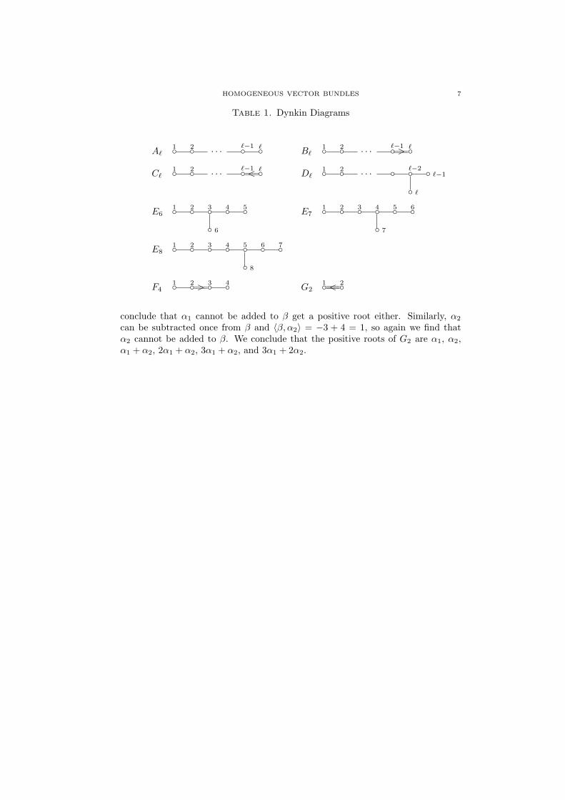
is dual to uP .The Dynkin diagram of a Lie groupG is a graph whose nodes are the simple roots.
The node corresponding to αi is connected to the node for αj by 〈αi, αj〉〈αi, αj〉lines. An inequality sign, > or < appropriately oriented, is superimposed on thelines connecting roots of different lengths. The connected components of a Dynkindiagram correspond to the simple factors ofG. For future reference we have includedthe Dynkin diagrams for the simple Lie groups below. The number adjacent to anode is the index i of the corresponding simple root αi.
The Cartan matrix [〈αi, αj〉] can be easily recovered from the diagram by usingthe fact that for simple roots αi 6= αj , 〈αi, αj〉 ≤ 0. The positive roots of G can beconstructed from the Cartan matrix by careful application of the above formula,
〈α, αj〉 = q − p
where p (resp. q) is the number of times αj can be added (resp. subtracted) fromα and still obtain a root.
For example, if G = G2, then 〈α1, α2〉 = −1, and 〈α2, α1〉 = −3. We cannotsubtract α1 from α2 (and vice versa) to get another root, so these negative numbersimply that α1 +α2, 2α1 +α2, and 3α1 +α2 are positive roots. Since we know howmany times we can subtract any simple root from one of these newly computedroots α, we can determine how many times we can add a simple root to α. Indeed,we find that for α = 3α1 + α2, we cannot subtract α2 but 〈α, α2〉 = −3 + 2 = −1,so β = 3α1 + 2α2 is another positive root. Similar considerations for other choicesyield no new roots. Finally, we check that no new root can be generated fromβ. Since we know α1 cannot be subtracted from β and 〈β, α1〉 = 6 − 6 = 0, we
HOMOGENEOUS VECTOR BUNDLES 7
Table 1. Dynkin Diagrams
A`1 2 · · · `−1 ` B`
1 2 · · · `−1 > `
C`1 2 · · · `−1 < ` D`
1 2 · · · `−2
`
`−1
E61 2 3
6
4 5 E71 2 3 4
7
5 6
E81 2 3 4 5
8
6 7
F41 2 > 3 4 G2
1 < 2
conclude that α1 cannot be added to β get a positive root either. Similarly, α2
can be subtracted once from β and 〈β, α2〉 = −3 + 4 = 1, so again we find thatα2 cannot be added to β. We conclude that the positive roots of G2 are α1, α2,α1 + α2, 2α1 + α2, 3α1 + α2, and 3α1 + 2α2.
8 DENNIS M. SNOW
3. Weyl Group
Geometrically, the linear map σα : E → E defined by
σα(λ) = λ− 〈λ, α〉αis a reflection of E through the hyperplane Eα = λ ∈ E | (λ, α) = 0 whichpreserves the weight lattice of G and the Killing form. The group of reflectionsgenerated by σα for α ∈ Φ is a finite group W called the Weyl group of G.
This group is in fact generated by the simple reflections σi = σαi , i = 1, . . . , `.The length of ω ∈W , denoted `(ω), is defined to be the minimal number t of simplereflections needed to express ω as a product of simple reflections, ω = σi(1) · · ·σi(t).
The Weyl chambers of E are the closures of the connected components of E \∪α∈Φ+Eα. The fundamental chamber is defined to be C = λ ∈ E | (λ, α) ≥0 for all α ∈ Φ+. Let λ ∈ E and consider a straight line from λ to a generic pointof C. If the hyperplanes crossed by this line are, in order, Eβ(1), . . . , Eβ(t), thenclearly ω = σβ(t) · · ·σβ(1) takes λ to C. This shows, in particular, that the Weylgroup W acts transitively on the Weyl chambers (it can be shown that this actionis also simple). We call ω(λ) the dominant conjugate of λ and sometimes denote itby [λ]. The index of λ is defined to be
ind(λ) = min`(ω) |ωλ ∈ Λ+Note that ω can also be written ω = σi(1) · · ·σi(t) where σi(j) is the simple
reflection σβ(t) · · ·σβ(j+1)σβ(j)σβ(j+1) · · ·σβ(t), j = 1, . . . , t. Therefore, if we defineΦ+
ω = Φ+ ∩ ω−1Φ−, then
Φ+ω = α ∈ Φ+ |ω(α) < 0 = σi(1) · · ·σi(j)αi(j) | j = 1, . . . , t
and `(ω) = |Φ+ω |, the number of elements in Φ+
ω . The index of λ can be similarlyidentified with the number of positive roots α > 0 such that (λ, α) < 0. We definethe index of a set of weights A ⊂ Λ to be the minimum of the indexes of weightsin A, indA = minindµ |µ ∈ A.
To find the index of a weight λ ∈ Λ, we write λ in the basis of fundamentaldominant weights: λ = n1λ1 + · · · + n`λ`. If the first negative coordinate is nj =〈λ, αj〉 < 0, then the weight σj(λ) will have index one less than λ. This is becauseσj permutes the positive roots other than αj and hence the number of negativeinner products, (λ, α) = (σjλ, σjα), is reduced by exactly one. In coordinates,σj(λ) = λ − njαj =
∑i(ni − cijnj)λi where the constants cij = 〈αi, αj〉 come
from the Cartan matrix [cij ]. This reflection is easy to calculate since cii = 2, sonj → −nj and only the coordinates ni ‘adjacent’ to nj in the Dynkin diagramfor G must be adjusted, nj → nj − cijnj . Repeating the above process on σjλ,i.e., reflecting it by σk where k is the index of the first negative coordinate, givesa weight of index 2 less than λ, and so on. Eventually we obtain the dominantconjugate of λ and the number of simple reflections used to get there is the indexof λ.
Since the Weyl group acts simply transitively on the Weyl chambers, the Weylgroup itself can be ‘coded’ into the set of vectors ωδ, ω ∈W , where δ = λ1+· · ·+λ`.The length of ω as well as its decomposition into a product of simple roots can bedetermined by applying the above algorithm to ωδ. In particular, `(ω) = ind(ωδ).
HOMOGENEOUS VECTOR BUNDLES 9
There is a unique longest element ω0 ∈W distinguished by the fact that ω0Λ+ =−Λ+. The length of ω0 equals the number of positive roots in the group:
`(ω0) = |Φ+| = dimG/B
Since ω20 = 1, ω0 induces a two-fold symmetry in W . For example, any ω ∈W can
be written ω = ω′ω0 with `(ω) = `(ω0)− `(ω′).For any set of indexes I ⊂ 1, . . . , ` we let WI be the subgroup of W generated
by the simple reflections σi, i ∈ I. We also denote this subgroup by WP where Pis the parabolic subgroup of G generated by I, since WP is isomorphic to the Weylgroup of the semisimple factor S(P ). A formula similar to that above holds for thelongest element ω1 ∈WP :
`(ω1) = |Φ+P | = dimP/B
More generally, for any dominant weight λ ∈ Λ we have the relations
ind(ωλ) ≤ `(ω) ≤ ind(ωλ) + dimPλ/B
and both extremes are taken on by some ω ∈ W . The upper bound is due tothe fact that ω′λ = λ for all ω′ ∈ WPλ
, and the maximum length of ω′ ∈ Pλ isdimPλ/B. Note that dimPλ/B is just the number of positive roots perpendicularto λ.
Let NG(T ) be the normalizer of T in G. For any representative n of a coset inNG(T )/T , it is clear that the linear map Ad(n)|t : t → t is independent of the choiceof representative. This correspondence between NG(T )/T and automorphisms oft actually defines an isomorphism from NG(T )/T to the Weyl group W definedabove, although we shall not try to justify this here. However, we shall make use ofthe fact that for every ω ∈W , there is a nω ∈ NG(T ) such that nωUαn
−1ω = Uωα. If
U =∏
α∈Φ− Uα is the maximal unipotent subgroup of G generated by the negativeroot groups, then it follows that
n−1ω Unω =
∏α∈Φ−
Uω−1α =∏
β∈Φ1
Uβ
∏γ∈Φ2
Uγ
where Φ1 = Φ− ∩ ω−1Φ− and Φ2 = Φ+ ∩ ω−1Φ− = Φ+ω . Note that |Φ2| = |Φ+
ω | =`(ω). This is the starting point for the following decomposition of G whose proofwe omit:
Theorem 3.1 (Bruhat Decomposition). Let G be a connected semisimple complexLie group, let B be a Borel subgroup of G, and let U ⊂ B be the maximal unipotentsubgroup. Then G decomposes into a disjoint union:
G =⋃
ω∈W
UnωB
where UnωB = UnσB if and only if ω = σ in W . Moreover, dimUnωB = `(ω) +dimB for ω ∈W .
This decomposition reflects a corresponding cellular decomposition of the homo-geneous space X = G/B. Indeed, the orbit Xω = U · (nωB) ⊂ X for ω ∈ W isisomorphic to
∏γ∈Φ+
ωUγ
∼= C`(ω) and the disjoint union of these orbits isX. A simi-lar decomposition can be obtained for X = G/P where P is any parabolic subgroupof G by using coset representatives ω(τ) ∈W of minimal length for τ ∈W/WP :
X =⋃
τ∈W/WP
Unω(τ)P
10 DENNIS M. SNOW
Since ω(τ) has minimal length, the dimension of the cell Xτ = Unω(τ)P is `(ω(τ)).Thus we find that the betti numbers, bi(X) = dimHi(X,R) = dimHi(X,R), satisfyb2i+1(X) = 0 and b2i(X) is the number of elements in τ ∈W/WP | `(ω(τ)) = i
A good way to determine the coset representatives ω(τ) for τ ∈ W/WP is toconsider the W -orbit of λP =
∑i/∈I λi where I is the set of indexes defining P .
The orbit is isomorphic to W/WP and for any ωλP ∈ W/WP a minimal cosetrepresentative is given by finding the sequence of simple reflections that take ωλP
to its dominant conjugate as above. One can construct the orbit of a dominantweight λ ∈ Λ+ directly by reversing the above algorithm: First, let L0 = λ anddefine Li for i ≥ 1 recursively as the set of weights σjµ where µ ∈ Li−1 and thej-th coordinate of µ is positive, 〈µ, αj〉 > 0. The weights in Li have index i. Ingeneral, a single weight in Li can come from many different weights in Li−1 andthis becomes a significant computational problem when the orbits are large. Thereare efficient ways to deal with this however, see [47].
Some simple examples to illustrate how these ideas can be applied:- b2(X) is the number of positive coordinates of λP , so b2(X) = rankG−|I|.
In particular, P is a maximal parabolic subgroup (λP = λi for some i) ifand only if b2(X) = 1.
- IfX = P` thenG is typeA` and λP = λ1. In this case, Li = σiσi−1 · · ·σ1λ1 =−λi + λi+1, and b2i = 1 for 0 ≤ i ≤ ` as expected.
- If X is an n-dimensional non-singular quadric hypersurface in projectivespace then G is of type B` (n = 2` − 1) or D` (n = 2` − 2) and againλP = λ1. For type B` we find Li = σiσi−1 · · ·σ1λ1 = −λi +λi+1 (L`−1 =−λ`−1 + 2λ`) and Ln−i = −Li so that b2i(X) = 1 for 0 ≤ i ≤ ` − 1.Type D` is the same except Ln/2 = L`−1 = −λ`−1 + λ`, λ`−1 − λ` andbn/2(X) = 2.

HOMOGENEOUS VECTOR BUNDLES 11
4. Irreducible Representations
Weyl’s theorem states that every G-module V can be decomposed into a directsum of irreducible G-modules. More precisely,
V ∼=t⊕
i=1
Vi ⊗ Ei
where the Vi are pairwise non-isomorphic irreducible G-modules and the Ei aretrivial G-modules. The dimension of Ei is called the multiplicity of Vi in V .Any G-invariant subspace W of V—for example, the image or kernel of a G-homomorphism—must be of the form
W ∼=t⊕
i=1
Vi ⊗ Fi
where the Fi are (possibly trivial) subspaces of Ei. A special case of this is knownas Shur’s Lemma: If φ : V → W is a G-homomorphism of irreducible G-modules,then φ is either trivial or an isomorphism.
We denote the weights of the G-module V by Λ(V ) ⊂ Λ. Recall from 2 that ifv is a weight vector for λ ∈ Λ(V ), then for all roots α ∈ Φ, Xαv is either 0 or hasweight λ+α. This leads to a partial ordering of the weights: we say µ < λ if λ−µis a positive linear combination (possibly zero) of positive roots. This ordering canbe applied to all of Λ, of course, and is compatible with the notation for positiveroots, α > 0.
Let λ ∈ Λ(V ) be a weight that is maximal with respect to the above partial orderand let v be the corresponding weight vector. Since Xαv = 0 for all positive rootsα > 0 by maximality, we see that the weights in the G-submodule generated by vλ
are all < λ. Notice also that such a v would be fixed by the maximal unipotentsubgroup U+ of G generated by the positive root groups Uα, α > 0. Let V U+
denote the set of fixed points of U+. The set of maximal weights Λmax(V ) in V
is thus Λ(V U+). We also refer to the weights Λmax(V ) as the highest weights of
V . Equivalently, if U denotes the usual maximal unipotent subgroup generated bythe negative root groups Uα, α < 0, then Λmax(V ) = −Λ(V ∗U ). This last equalityallows us to extend the definition of maximal weights in a meaningful way to anyP -module where P is a parabolic subgroup of G, see §8.
If V is irreducible, any two maximal weights, λ, µ ∈ Λmax(V ), would both haveweight vectors that generate all of V , and so µ < λ and λ < µ. Therefore, forany irreducible G-module there is a unique maximal weight λ. The G-moduleV is in fact uniquely determined by λ and we use the notation V λ to make thisassociation explicit. The notation for the weights Λ(V λ) will be shortened to Λ(λ).Since the weights Λ(λ) and their multiplicities are invariant under the action ofthe Weyl group, see §2, they are determined by their dominant conjugates: IfΛ+(λ) = Λ(λ)∩Λ+, then Λ(λ) = W ·Λ+(λ). In particular, since σλ < λ for σ ∈W ,λ itself must be dominant. We refer to the weights Λ+(λ) as the subdominantweights of the representation.
The subdominant weights Λ+(λ) are easily determined. Starting with λ, wecollect all weights of the form λ − α, α > 0, that are dominant into a list L1.We know from §2 that L1 must consist of subdominant weights, L1 ⊂ Λ+(λ).Continuing in this way, we create a list Lk+1 consisting of all weights of the form
12 DENNIS M. SNOW
µ − α, µ ∈ Lk, α > 0, that are dominant. Again, Lk+1 ⊂ Λ+(λ). We eventuallyreach the state where Lt+1 = ∅. It is clear that all subdominant weights musthave the form µ = λ − β1 − · · · − βk. However, the ‘path’ from λ to µ may, ingeneral, leave the fundamental chamber, depending on the roots β1, . . . , βk andtheir order. Nevertheless, it can be shown there is always a path from λ to anysubdominant weight µ that passes through only dominant weights so that Λ+(λ) =λ ∪ L1 ∪ · · · ∪ Lt, see, e.g., [41].
While the above discussion shows how to reconstruct the weights of any repre-sentation with minimal effort, its says nothing about how to determine the multi-plicities of the weights. There are several formulas which give these multiplicities,but they involve a fair amount of computation compared to the above procedure.Weyl’s character formula is the simplest to write:
χ(λ) =∑
ω∈W (−1)`(ω)eω(λ+δ)∑ω∈W (−1)`(ω)eω(δ)
where χ(λ) = Trφ =∑
µ∈Λ(λ)mµeµ is the character of the representation of φ :
g → GL(V λ) and δ = λ1 + · · · + λ`. The symbols eµ are to be manipulated usingthe usual rules of exponents. The multiplicity of µ in V λ is the coefficient mµ
of eµ in the resulting quotient which is computed like a quotient of polynomials.This formula is not very practical for computing multiplicities for groups of highrank since the size of W is exponential in ` making the above sums and quotientdifficult to handle. Freudenthal’s multiplicity formula is recursive and serves thispurpose much better, see [27, 41]. Using a limiting process, Weyl derived from hischaracter formula the following expression for the dimension of a representationwhich is relatively easy to compute:
dimV λ =∏
α>0〈λ+ δ, α〉∏α>0〈δ, α〉
Writing λ =∑`
i=1 n(λi)λi and α =∑`
i=1mi(α)αi, the dimension formula becomes
dimV λ =∏α>0
[1 +
∑`i=1 ni(λ)mi(α)∑`
i=1mi(α)
]Recall from §1 that the denominators in this expression are the heights of the roots,h(α) =
∑`i=1mi(α).
Let V be a G-module and let V ∗ denote the dual module. The action of G onf ∈ V ∗ is defined by (g · f)(v) = f(g−1 · v) for v ∈ V so that the weights of V ∗ arethe negatives of the weights of V : Λ(V ∗) = −Λ(V ). If V = V λ is irreducible withhighest weight λ, then it is clear that −λ is the ‘lowest’ weight of V ∗ in the sensethat −λ− α is not a weight of V ∗ for any positive root α > 0. Let ω0 ∈W be theunique Weyl group element that takes Λ+ to −Λ+, see §2. Since ω0Λ(V ∗) = Λ(V ∗)and ω0Φ+ = Φ−, it follows that −ω0λ must be the highest weight of V ∗ andV ∗ = V −ω0λ.
The involution −ω0 defines an involution of the Dynkin diagram of G. For groupswith diagram components lacking two-fold symmetry, i.e., whose components havetypes B`, C`, E7, E8, F4, and G2, this involution must be trivial and −ω0 = 1. Forcomponents of type A` the involution −ω0 is given by λi ↔ λ`−i+1, 1 ≤ i ≤ `, fortype D` it is given by λ`−1 ↔ λ`, and for E6 it is given by λ1 ↔ λ6, λ2 ↔ λ5.
HOMOGENEOUS VECTOR BUNDLES 13
5. Basic Concepts of Vector Bundles
Let X be a connected compact complex manifold that is homogeneous undera complex Lie group G so that X ∼= G/P where P is the isotropy subgroup of apoint x0 ∈ X. A holomorphic vector bundle π : E → X is homogeneous if thegroup of bundle automorphisms of E acts transitively on the set of fibers of E.We say that E is homogeneous with respect to G if the action of G on X lifts toa compatible action of G on E via holomorphic bundle automorphisms. If G is aconnected, simply-connected semisimple complex Lie group, then a homogeneousvector bundle π : E → X is always homogeneous with respect to G. This is notnecessarily the case for other types of groups. We shall always assume that E ishomogeneous with respect to G.
The isotropy subgroup P acts linearly on the fiber E0 = π−1(x0). Consider theaction map
G× E0µ−→ E
defined by µ(g, z) = g · z. Since G acts transitively on X, the map µ is clearlysurjective. The fibers of µ are the orbits of P on G×E0 under the diagonal action(g, z) → (gp−1, p · z), p ∈ P . In fact, we may represent any point in E as anequivalence class [g, z] for (g, z) ∈ G ×P E0 where [gp, z] = [g, p · z] for all p ∈ P .In this way E is isomorphic to the quotient
E = G×P E0 = (G× E0)/P
Conversely, given a holomorphic representation P → GL(E0), E = G ×P E0 is aholomorphic vector bundle over X that is homogeneous with respect to G. Thebundle map π : E → X is given by projection, π([g, z]) = gP ∈ G/P . Thus, theholomorphic vector bundles on X that are homogeneous with respect to G are inone-to-one correspondence with holomorphic representations P → GL(E0) and twosuch bundles are isomorphic if and only if the representations of P are conjugatein GL(E0).
Let q : G → G/P be the quotient map. Notice that the pull-back q∗E isisomorphic to G × E0 and the bundle map q∗E → E is simply the action mapµ. Given a holomorphic section of E, its pull back to q∗E ∼= G × E0 defines aholomorphic map s : G → E0 such that s(gp−1) = p · s(g). Conversely, any suchfunction defines a section of E. Therefore,
H0(X,E) ∼= s : G→ E0 | s(gp−1) = p · s(g) for all g ∈ G, p ∈ PThe latter set of functions on G has a natural G-module structure and is knownas the induced G-module of the P -module E0, denoted E0|G. The evaluation mapdefines a P -module homomorphism ev0 : E0|G −→ E0, ev0(s) = s(1), that satisfiesthe following universal property (see for example [11]):
Proposition 5.1 (Universality). If W is a finite dimensional G-module and φ :W → E0 is a P -module homomorphism, then there exists a unique G-module ho-momorphism ψ : W → E0|G such that φ ψ = ev0.
The map ψ is straightforward to construct. For w ∈ W , define ψ(w) : G → E0
by ψ(w)(g) = φ(g−1 · w). Since ψ(w)(gp−1) = p · ψ(w)(g) for all p ∈ P , we seethat ψ(w) does indeed lie in E0|G. In fact, it is often convenient to start witha G-module V and a P -module homomorphism φ : V → E0 and then constructsections s : G→ E0 for G×P E0 by defining s(g) = φ(g−1 · v) for v ∈ V .
14 DENNIS M. SNOW
Another useful property of induced modules is the following.
Proposition 5.2 (Transitivity). If Q is a closed complex subgroup of G containingP , then E0|G ∼= E0|Q|G.
Let Y = G/Q and let τ : X → Y be the natural coset map with fiber Z = Q/P .Since the direct image sheaf, τ∗E, is isomorphic to H0(Z,E|Z)⊗OY
∼= E0|Q⊗OY ,the above statement simply expresses the fact that H0(X,E) ∼= H0(Y, τ∗E). Thedegree to which the bundle E is ‘trivial’ is reflected in the degree to which theP -module E0 can be extended to larger subgroups of G. For example, if E0 canbe extended to a Q-module, then E is the pull back of the bundle G×Q E0 over Yunder the coset map X → Y and E|Z is isomorphic to the trivial bundle, Z × E0.In particular, the P -module E0 can be extended to a G-module if and only if thebundle E is globally trivial, E ∼= X × E0.
The above evaluation map, ev0, of course, corresponds to the usual evaluationmap of sections, ev : X × V → E defined by ev(x, s) = s(x), x ∈ X, s ∈ V =H0(X,E). The bundle E is said to be spanned by global sections (or simplyspanned) if ev is surjective,
X × Vev−→ E −→ 0
If E is spanned, then the dual map, ev∗, imbeds E∗ into X × V ∗. Composingev∗ with projection onto V ∗ yields a map
ν : E∗ −→ V ∗
which imbeds the fibers E∗0 of E∗ as linear subspaces of V ∗ and sends the zerosection ZX of E∗ to the origin of V ∗. By projectivizing we also obtain a map
Pν : P(E∗) −→ P(V ∗)
which imbeds the fibers P(E∗0 ) of p : P(E∗) → X linearly into P(V ∗). Notice that νthus defines an equivariant map of X to a Grassmann manifold by sending x ∈ Xto the point represented by the subspace ν(E∗x) ⊂ V ∗. In the case where E isa line bundle, the projectivization P(E∗) is isomorphic to X, and this map to aGrassmann manifold coincides with Pν giving the canonical map of X to projectivespace defined by the sections of E.
A canonical hermitian metric for E can be induced from a hermitian metricin V as follows. First observe that a hermitian metric, similar to the case ofsections, is given by a map hE : G → GL(E0) satisfying hE
t = hE and hE(gp) =ϕ(p)thE(g)ϕ(p) for g ∈ G, p ∈ P where ϕ : P → GL(E0) defines the P -modulestructure of E0. The latter condition ensures that for [g, (z, w)] ∈ G×P (E0 × E0)the hermitian product
(z, w)E = wthE(g)zis well-defined. Choosing a basis of weight vectors s1, . . . , sm for V and a dual basisη1, . . . , ηm for V ∗ allows us to write ν as ν[g, z] =
∑k z(sk(g))ηk for [g, z] ∈ G×PE0.
A metric hE∗ for E∗ is then defined by
wthE∗(g)z = ν[g, w]tν[g, z] =m∑
k=1
w(sk(g))z(sk(g))
HOMOGENEOUS VECTOR BUNDLES 15
where the transpose is from a column vector to a row vector. Equivalently,
hE∗(g) =m∑
k=1
sk(g)sk(g)t
The metric for E is
hE = (htE∗)
−1 =
(m∑
k=1
sk(g)sk(g)t
)−1
This construction does not depend on the bundle being homogeneous—similardefinitions for hE∗ can be made using local trivializations of E∗ instead—and canbe extended to any vector bundle E on X as long as X is a projective manifold:Let L be an ample line bundle on X such that E⊗L is spanned. The metrics hE⊗L
and hL are defined as above, and then a metric for E is given by hE = (hE⊗L)h−1L .
The inverse image under the map ν of a ball centered at the origin in V ∗ gives atube neighborhood of the zero section ZX in E∗. The Levi form, L, of the boundaryof this tube retains the positive eigenvalues of the ball it came from. Therefore,there can be at most k non-positive eigenvalues of L where k is the maximum fiberdimension of ν. This number k can also be determined from the eigenvalues of thecurvature form ΘE = ∂(h−1
E ∂hE), see §8. Such information has implications forthe cohomology of E and its symmetric powers E(m). For example, the theoremof Andreotti-Grauert [1] in this case states that Hq(X,E(m)) = 0 for q > k if m issufficiently large.
Maps similar to ν and Pν can be constructed in a slightly more general setting.Let P(E∗) be the projectivization of E∗, that is, the quotient of the natural C∗action on E∗ \ ZX , and let ξE → P(E∗) be the associated tautological line bundlethat is isomorphic to the hyperplane section bundle, OP(E∗0 )(1), on the projectivespace fibers P(E∗0 ) of p : P(E∗) → X. As manifolds, E∗ \ ZX
∼= ξE \ ZP(E∗) whereZP(E∗) is the zero section of ξE . Moreover, for any positive integer m there isa natural isomorphism of sheaves, p∗ξm
E∼= E(m). Instead of requiring that E∗ be
spanned, we may assume the weaker condition that some power, say ξmE , is spanned
over P(E∗). Letting Vm = H0(P(E∗), ξmE ) ∼= H0(X,E(m)) we obtain the maps
Pνm : P(E∗) −→ P(V ∗m) and νm : E∗ −→ V ∗m
The latter is obtained from the former by lifting. The fibers of νm are finite on thefibers E∗0 so the analysis of the eigenvalues of the Levi form of a tube neighborhoodgoes through as before, see §7.3. These ideas lead to the the notion of k-ampleness,see [53].
Definition 5.3. A line bundle L → X is k-ample if some power Lm is spannedand the fibers of Pνm : X → P(V ∗m) have dimension at most k. A vector bundle Eis k-ample if ξE → P(E∗) is k-ample.
Classically, a line bundle L → X is said to be very ample if Pν : X → P(V ∗) isan imbedding and L is said to be ample if some power Lm is very ample. Thus,0-ample in the above sense is equivalent to ample in the classical sense (if the fibersof Pνm are zero dimensional, some higher value of m yields an imbedding).
Most of the familiar vanishing theorems for ample bundles have versions fork-ample bundles. For example:
16 DENNIS M. SNOW
Theorem 5.4 ([36, 53]). If E → X is a k-ample vector bundle, then Hp,q(X,E) =Hq(X,Ωp
X ⊗ E) = 0 for p+ q ≥ k + rankE + dimX.
A homogeneous vector bundle E = G ×P E0 is said to irreducible if the rep-resentation of P on E0 is irreducible. For example, any homogeneous line bundleon G/P is necessarily irreducible since the representation of P is one-dimensional.Since a Borel subgroup B ⊂ G is solvable, an irreducible representation of B is nec-essarily one-dimensional and so homogeneous line bundles are the only irreduciblehomogeneous vector bundles on G/B.
We shall see that irreducible homogeneous bundles often have the sharpest the-orems and the most detailed formulas associated to them. Unfortunately, manyinteresting bundles are not irreducible, for example, most tangent bundles on G/P .Nevertheless, it is it is often possible to draw conclusions about an arbitrary ho-mogeneous vector bundle E = G×P E0 from the irreducible case by considering afiltration of E0 by P -submodules, as follows.
If LP is a Levi-factor of P , then the module E can be decomposed into a directsum irreducible LP -modules, E0 = F1 ⊕ · · · ⊕ Ft, see §1. Furthermore, since theunipotent radical, UP , is normal in P and acts on E0 in a ‘triangular’ fashion, itis clear that these LP -irreducible factors can be arranged (non-uniquely) such thatUPFi ⊂ Fj with j ≥ i. Therefore, E0 has a filtration by P -submodules
E0 ⊃ E1 ⊃ · · · ⊃ Et ⊃ Et+1 = 0
such that Ei/Ei+1∼= Fi is an irreducible P -module with maximal weight µi, i ≤
i ≤ t.
Definition 5.5. The maximal weights of a P -module E0, denoted Λmax(E0), arethe maximal weights of the irreducible factors associated to a filtration of E0 byP -submodules, as above.
Equivalently, we could define Λmax(E0) = −Λ(E∗0U ), where U ⊂ P is the maxi-
mal unipotent subgroup of G generated by all the negative root groups, see §4.
HOMOGENEOUS VECTOR BUNDLES 17
6. Line Bundles
We now concentrate on the case of homogeneous line bundles. The followingwell-known lemma is the first step in classifying projective homogeneous manifolds.
Lemma 6.1. Let X be a compact complex space and let R be a connected solvablecomplex Lie group acting holomorphically on X. Assume that with respect to thisaction X is equivariantly imbedded into some complex projective space PN . ThenR has a fixed point on X, that is, there is a point x ∈ X such that r · x = x for allr ∈ R.
Proof. By Lie’s Theorem, R stabilizes a flag of linear subspaces
P0 ⊂ P1 ⊂ · · · ⊂ PN = PN
where Pk∼= Pk, 0 ≤ k ≤ N . Let Xk = X ∩ Pk and define X−1 = ∅. Let k be
the least integer for which Xk 6= ∅ and Xk−1 = ∅. Then Xk is a compact complexspace contained in Pk \ Pk−1
∼= Ck. Therefore, Xk must be a finite set of pointsstabilized by R. Since R is connected, it must fix each of the points in Xk.
Recall that if L is an ample line bundle on X, then the sections Vm = H0(X,Lm)of some power of L imbed X into P(V ∗m). If L is homogeneous with respect to Gthen G acts linearly on Vm and the imbedding is naturally G-equivariant. Thefollowing proposition shows that there is a significant restriction on the type ofspaces for which this can occur.
Proposition 6.2. Suppose there exists an ample homogeneous line bundle on aconnected homogeneous compact complex manifold X. Then X is homogeneousunder a connected, simply-connected, semisimple complex Lie group G, X = G/P ,and the isotropy subgroup P is parabolic.
Proof. Let X be homogeneous under a complex Lie group G such that there existsa G-equivariant imbedding of X into some projective space. Since X is connectedwe may assume G is connected. Let G = R · S be a Levi-Malcev decompositionof G where R is the radical of G (a maximal connected normal solvable subgroup)and S is a connected semisimple complex subgroup of G. By Lemma 6.1, R fixes apoint in X. But then R fixes every point of X since R is normal in G. Hence, thesemisimple group S acts transitively on X. It is an easy matter to lift the actionto the universal cover S of S which is still a semisimple complex Lie group. Nowlet B be a Borel subgroup of S. Again by 6.1, B fixes some point in X and thus iscontained in the isotropy subgroup of that point.
From now on we shall assume that X = G/P where G is a connected simply-connected semisimple complex Lie group and P is a parabolic subgroup. Our nextgoal is to understand the additive group of holomorphic line bundles, Pic(X), onX.
Let L → X = G/P be a homogeneous line bundle on X. Then L = G ×P Cdetermines a homomorphism λ : P → GL(1,C) ∼= C∗. Since λ|SP
and λ|UPare
necessarily trivial, we see that λ is determined by its restriction to TP , which inturn defines a weight λ ∈ Λ that is perpendicular to the weights of P : (λ, α) = 0for all α ∈ P . Conversely, starting with weight λ perpendicular to the weights of P ,we can construct a character λ : P → C∗ that defines a homogeneous line bundle
18 DENNIS M. SNOW
on X. Thus we see that the homogeneous line bundles on X are in one-to-onecorrespondence with the set of weights
ΛX = λ ∈ Λ | (λ, α) = 0 for all α ∈ ΦP which we call the weights of X. Note that (λ, α) = 0 for all α ∈ ΦP is equivalentto 〈λ, αi〉 = 0 for all i ∈ I, where I is the subset of indexes that defines P . Thus,with respect to the basis of fundamental dominant weights, the weights of X arethe weights with i-th coordinate zero for i ∈ I.
A remarkable fact about line bundles on X = G/P is that they must always behomogeneous with respect to G. This is certainly not the case for vector bundlesof higher rank. We first prove a lemma.
Lemma 6.3. Let X = G/P with G semisimple and P a parabolic subgroup. Thenπ1(X) = 0 and H1(X,OX) = 0.
Proof. Since X is compact, we need only show that π1(X) = 0. For if H1(X,OX) ∼=H0(X,ΩX) were then not also trivial, we could construct non-constant holomorphicfunctions on X by integrating closed holomorphic forms. By Theorem 3.1, there isan open dense subset of X isomorphic to Cn. Since the inclusion map of this cellinto X lifts to an inclusion map of the cell to a dense open subset of the universalcover π : X → X, we see that π must be one-to-one and X is simply-connected.
Theorem 6.4. Let X = G/P with G semisimple and P a parabolic subgroup. IfL is any holomorphic line bundle on X, then L is homogeneous with respect to G.In particular, Pic(X) ∼= ΛX .
Proof. Holomorphic line bundles on X correspond to elements in H1(X,O∗X). The
short exact sequence 0 → Z → OX → O∗X → 0 leads to natural mapsH1(X,OX) →
H1(X,O∗X) → H2(X,Z), the latter sending a holomorphic line bundle to its topo-
logical class. Since H2(X,Z) is discrete and G is connected, the topological classof g∗L must be the same as L. By Lemma 6.3, H1(X,OX) = 0, so the two bundlesL and g∗L are in fact isomorphic as holomorphic line bundles. Since there are nonon-trivial homomorphisms G→ C∗, these isomorphisms for g ∈ G define an actionof G on L by bundle automorphisms and L is homogeneous with respect to G.
Now that we know that line bundles on X = G/P correspond to weights ΛX ,we can investigate how various properties of the line bundle can be translated intoproperties of weights. The next theorem addresses the question of when a linebundle is spanned or is ample.
Theorem 6.5 (Borel-Weil [42]). Let L be a holomorphic line bundle on X = G/Pwhere G is semisimple and P is a parabolic subgroup defined by a set of indexes I.Let λ =
∑i/∈I niλi ∈ ΛX be the weight associated to L. Then
(1) L is spanned at one point of X iff L is spanned at every point of X iffni ≥ 0 for i /∈ I (i.e. iff λ is dominant).
(2) L is ample iff L is very ample iff ni > 0 for i /∈ I.(3) If λ is dominant, then H0(X,L) is isomorphic to the irreducible G-module
V λ.(4) If λ is not dominant, then H0(X,L) = 0.
Proof. 1. (⇒) Let s ∈ V = H0(X,L) be a section that is non-zero at x ∈ Xand let y = g · x, g ∈ G, be any other point of X. Here s corresponds to a
HOMOGENEOUS VECTOR BUNDLES 19
function s : G → C such that s(gp−1) = λ(p)s(g) for all g ∈ G and p ∈ P (see§5). Since L is homogeneous with respect to G, g · s is also a section of L thatis non-zero at y: g · s(y) = s(g−1y) = s(x). It follows that the P -equivariantevaluation map ev0 : V → C is non-zero. Let s be a weight vector in V of weight µsuch that ev0(s) = s(1) 6= 0 and let W be the irreducible G-submodule generatedby s. Now for all t ∈ T , (t · s)(1) = s(t−1 · 1) = µ(t)s(1). On the other hand,s(1 · t−1) = λ(t)s(1) for all t ∈ T ⊂ P , so µ = λ. Moreover, since λ is perpendicularto ΦP , ev0(Xαs) = λ(Xα) ev0(s) = 0 for all roots α ∈ ΦP . Since the kernel of ev0
is P -invariant and all the negative roots are in ΦP , we conclude that s is a maximalweight vector and W ∼= V λ. Moreover, by Proposition 5.1, ev0 : V → C factorsthrough the projection of W onto its maximal weight space C · s. In particular, λis dominant.
(⇐) Let λ ∈ Λ+X be dominant, let v ∈ V λ be a maximal weight vector with
weight λ, and let f ∈ (V λ)∗ be dual to v: f(v) = 1 and f(u) = 0 for u in any otherweight space. Since λ is perpendicular to the weights of P , it can be extendedto a character λ : P → C∗. For X ∈ p, we have X.v = λ(X)v + u(X) whereu(X) is a linear combination of vectors from weight spaces other than λ. Hence,f(p.v) = λ(p)f(v) for all p ∈ P . Define a map s : G→ C by s(g) = f(g−1.v). Thens(gp−1) = λ(p)s(g) for all g ∈ G and p ∈ P , see Proposition 5.1. Hence, there is anon-zero section of the line bundle on G/P defined by λ.
2. Since Lm corresponds to the weight mλ, it is clear that we need only showthat L being very ample is equivalent to ni > 0 for all i /∈ I. We may also assumeλ is dominant, so that L is spanned.
Suppose nj = 0 for some j /∈ I. Let J = I ∪ j and let Q be the parabolicsubgroup defined by J . Since the roots of Q are perpendicular to the weight λ, thecharacter λ can be extended to Q. This implies that L is the pull-back of a linebundle on G/Q, and hence L is not very ample, see §5.
Conversely, if L is not very ample then the map given by the sections of L,π : G/P → G/Q, is not an imbedding. The character λ therefore extends to aparabolic subgroup Q that properly contains P . Hence there is a simple root αj
not in P such that nj = 〈λ, αj〉 = 0.3. Let W ∼= V µ be any non-trivial irreducible G-submodule of V . There must be
at least one weight vector s in W such that ev0(s) 6= 0. Otherwise, for any weightvector s in W , ev0(g · s) = 0 for all g ∈ G and hence s = 0, a contradiction. Bypart 1, we know that W ∼= V λ, so µ = λ, and ev0 : V → C factors through theprojection of W onto C · s. Since W is arbitrary, we conclude that V ∼= V λ.
4. This is a simple consequence of 1.
The proof of 2 above shows how to describe the map of X = G/P to projectivespace defined by the sections of a spanned line bundle.
Corollary 6.6. Let L be a line bundle on X = G/P defined by a weight λ ∈ ΛX .Assume that L is spanned by global sections so that λ is dominant. Then the mapπ : X → Y ⊂ P(V ∗) defined by the sections of L, V = H0(X,L), is a homogeneousfibration G/P → G/Q where Q is the parabolic subgroup of G defined by the simpleroots perpendicular to λ. In particular, λ defines a very ample line bundle L′ on Yand L = π∗L′.

20 DENNIS M. SNOW
7. Curvature
We now discuss some aspects of the curvature of a homogeneous vector bundleE = G ×P E0 on X = G/P where P is a parabolic subgroup of G. We firstcompute the curvature form ΘE = ∂(h−1
E ∂hE) associated to a natural left-invarianthermitian metric hE on E. Since ΘE is also left-invariant, it is determined by itsform at the identity coset. To carry out this computation, we rely on the notationof §2 and §5, and use local coordinates xα, α ∈ ΦX , defined for g ∈ G near 1 by
g =∏
α∈ΦX
exp(xαXα)
In the next theorem we assume that E is spanned by global sections. Thecurvature form of an arbitrary homogeneous vector bundle E can then be derived,as usual, by ΘE = ΘE⊗L − IEΘL where L is an ample line bundle on X such thatE ⊗ L is spanned by global sections.
Theorem 7.1. Let E = G ×P E0 be a homogeneous vector bundle on X = G/Pwhere P is a parabolic subgroup of G. Assume E is spanned by global sections so thatthe P -module homomorphism φ : V = H0(X,E) → E0 is surjective. Let v1, . . . , vm
be a basis of weight vectors for V and e1, . . . , er for E0 such that φ(vk) = ek,1 ≤ k ≤ r. Then there is a natural left-invariant hermitian metric for E whoseassociated curvature form is given at the identity coset by
ΘE =∑
α,β∈ΦX
∑k>r
φ(Xα · vk)φ(Xβ · vk)tdxα ∧ dxβ
Proof. As in §5, we define sections of E, sk : G → E0, by sk(g) = φ(g−1 · vk) for1 ≤ k ≤ m so that a hermitian metric hE : G→ R for E is given by
hE =( m∑
k=1
skstk
)−1
Let
A =m∑
k=1
skstk = ht
E∗
Since ∂hE = −hE(∂A)hE , we obtain
ΘE = ∂(h−1E ∂hE) = (∂∂A)hE − (∂A)hE ∧ (∂A)hE
Note that hE(1) = I, sk(1) = ek, and∂sk
∂xα(1) = φ(−Xα · vk)
We abbreviate φ(Xα · vk) by φα,k so that at the identity coset the above expressionfor ΘE becomes
ΘE = ∂∂A− ∂A ∧ ∂A
=∑
α,β∈ΦX
m∑k=1
φα,kφtβ,k −
m∑j,k=1
φα,ketkejφt
β,j
dxα ∧ dxβ
=∑
α,β∈ΦX
∑k>r
φα,kφtβ,kdxα ∧ dxβ
HOMOGENEOUS VECTOR BUNDLES 21
as claimed.
The curvature ΘE can be written in a particularly simple way. Let F0 denotethe kernel of φ : V → E0, i.e., the subspace of V spanned by vk, k > r. For α ∈ ΦX
define linear maps φα : F0 → E0 by
φα(v) = φ(Xα · v)and maps φt
α : E0 → F0 dual to φα with respect to the above bases. Then
ΘE =∑
α,β∈ΦX
φαφtβdxα ∧ dxβ = Ψ ∧Ψt
whereΨ =
∑α∈ΦX
φαdxα
This description makes it easier to see the properties of the curvature form
ΘE(z) = ztΘE z
for z ∈ E0.
Definition 7.2. We say that ΘE(z) is positive semidefinite if ΘE(z)(η, η) ≥ 0for all η ∈ (TX)0. The kernel of ΘE(z) is the subspace of η ∈ (TX)0 such thatΘE(z)(η, η) = 0. The flatness of ΘE is defined to be
flΘE = maxz∈E0\0
dim kerΘE(z)
If ( , ) denotes the hermitian metric on V with respect to the basis vk, 1 ≤ k ≤ m,then
ΘE(z) =∑
α,β∈ΦX
(φtαz, φ
tβz)dxα ∧ dxβ
and for η =∑
α∈ΦXηα∂/∂xα ∈ (TX)0,
ΘE(z)(η, η) =∑
α,β∈ΦX
(ηαφtαz, ηβφ
tβz) = |Ψt(z)η|2
Thus we may conclude the following.
Corollary 7.3. If E is spanned by global sections, the curvature form ΘE(z) ispositive semidefinite for all z ∈ E0, its kernel equals the kernel of Ψt(z) : (TX)0 →F0, Ψt(z) =
∑α∈ΦX
φtα(z)dxα, and the flatness of ΘE is given by
flΘE(z) = maxz∈E0\0
dim kerΨt(z)
The ‘flatness’ of ΘE is related to the ‘ampleness’ of the bundle E, see §8.
Remark 7.4. It is possible to construct a holomorphic connection θE and its asso-ciated curvature form ΘE = ∂θE for a homogeneous vector bundle E = G ×P E0
using a basis of left-invariant forms, their duals, and the representation of p on E0,see, e.g., [24, 22]. In general, such a connection is a metric connection only whenthe representation of P on E0 is irreducible. In this case, the resulting curvatureform ΘE is also non-degenerate, and its signature is given by the index of the maxi-mal weight of E0, see [24, Theorem 4.17]. While some homogeneous vector bundles(e.g., line bundles) are known to be irreducible, many other important bundles (e.g.,most tangent bundles) are not.
22 DENNIS M. SNOW
7.1. Curvature of tangent bundles. As an example, let us compute the curva-ture form for the holomorphic tangent bundle E = TX of a homogeneous manifoldof the form X = SL(` + 1,C)/P where P is parabolic subgroup. In this caseE0 = (TX)0 can be viewed as a vector space of certain strictly upper triangularmatrices by identifying the root vectors Xα, α ∈ ΦX , with the elementary matriceseµν indexed as follows. Define ‘row’ and ‘column’ indexes by
Rν = i | eiν = Xα for some α ∈ ΦXCµ = j | eµj = Xα for some α ∈ ΦX
Both Rν and Cµ may be empty, but if they are not then they have the formRν = 1, . . . , rν and Cµ = cµ, . . . , ` + 1. In fact, if I is the set of indexes thatdefines P , then
rν = maxi ∈ I | i < ν, cµ = mini ∈ I | i ≥ µ+ 1
For α ∈ ΦX we have Xα = eµν if and only if 1 ≤ µ ≤ ` + 1 and ν ∈ Cµ (or1 ≤ ν ≤ `+ 1 and µ ∈ Rν). Note that µ ∈ Rν if and only if ν ∈ Cµ.
The space of sections V = H0(X,TX) is isomorphic to the Lie algebra of G =SL(` + 1,C). The map φ : V → (TX)0 is just the natural projection of matricesand the module structure is given by Lie brackets of matrices. Thus, if Xα = eµν ,and vk = eij , then ‘k > r’ means i /∈ Rj (or j /∈ Ci), and
φα,k = φ(Xα · vk) = φ([eµν , eij ])
=
eµj if i = ν and j ∈ Cµ \ Cν
−eiν if j = µ and i ∈ Rν \Rµ
0 otherwise
Let us write xµν for the coordinate xα, and let fρσµν denote the r× r elementary
matrix eµνetρσ (the transpose here is of a column vector to a row vector not the
usual transpose of a matrix, and r = dimX). Let β ∈ ΦX be another root withXβ = eρσ. If ν = σ then
φαφtβ =
∑k>r
φα,kφtβ,k =
∑j∈Cµ∩Cρ\Cν
fρjµj
while if µ = ρ, thenφαφt
β =∑
i∈Rν∩Rσ\Rµ
f iσiν
Finally, if ν ∈ Rσ \ Rρ and ρ ∈ Cµ \ Cν , then φαφtβ = −fνσ
µρ , while if σ ∈ Rν \ Rµ
and µ ∈ Cρ \ Cσ, then φαφtβ = −fσν
ρµ . For any other combination of µ, ν, ρ and σ,φαφt
β = 0. Let δpq have the value 1 if p = q and 0 otherwise. Define εstpq to be 1 if
s ∈ Rt \Rq and q ∈ Cp \Cs, and to be 0 otherwise. According to Theorem 7.1 andthe above description of φαφt
β we obtain
ΘTX=
∑µ∈Rν ,ρ∈Rσ
[δνσ
∑j∈Cµ∩Cρ\Cν
fρjµj + δµρ
∑i∈Rν∩Rσ\Rµ
f iσiν
− ενσµρf
νσµρ − εσν
ρµfσνρµ
]dxµν ∧ dxρσ
HOMOGENEOUS VECTOR BUNDLES 23
Another way to express this is to view ΘTXas a r× r matrix of (1, 1)-forms and
let Θstpq denote the entry in the pq-row and st-column of ΘTX
. Then
Θstpq = δqt
∑ν /∈Rq
dxpν ∧ dxsν + δps
∑µ/∈Cp
dxµq ∧ dxµt
− εstpqdxps ∧ dxqt − εst
pqdxqt ∧ dxps
The map φα : F0 → E0 is given by
φα(v) =∑
j∈Cµ\Cν
vνjeµj −∑
i∈Rν\Rµ
viµeiν
where v =∑
i/∈Rjvijeij ∈ F0. The dual φt
α : E0 → F0 is
φtα(z) =
∑j∈Cµ\Cν
zµjeνj −∑
i∈Rν\Rµ
ziνeiµ
where z =∑
i∈Rjzijeij ∈ E0. Thus, for p ∈ Rq,
Ψt(epq) =∑
ν /∈Rq
eνqdxpν −∑
µ/∈Cp
epµdxµq
It follows that the kernel of Ψt(epq) is the set of tangent vectors η whose coordinatesηµq = 0 for µ /∈ Cp and ηpν = 0 for ν /∈ Rq. Therefore
dim kerΨt(epq) = dimX − (`+ cp − rq − 1)
The maximum of this kernel dimension for z ∈ (TX)0 is achieved at z = ei,i+1,i ∈ I, where ci = i+ 1 and ri+1 = i, and thus
flΘE = maxz∈(TX)0\0
dim kerΨt(z) = dimX − `
a fact that will be recalled in §8. Notice that among these examples the only casewhere ΘE(z) is positive definite is for complex projective space, X = P`.
Two extreme examples of such homogeneous spaces are the flag manifold anda Grassmann manifold. The flag manifold is the space of all full ‘flags’ of linearsubspaces in (`+ 1)-space: V0 ⊂ V1 ⊂ · · · ⊂ V`+1, dimVi = i. For this manifold, Pis a Borel subgroup and I = 1, . . . , `. The row and column indexes are
Rν = 1, . . . , ν − 1, Cµ = µ+ 1, . . . , `+ 1which are easily applied to the above formulas for ΘTX
.For the Grassmann manifold X = Gr(ω, `+ 1) of ω-planes in (`+ 1)-space, P is
a maximal parabolic subgroup and I = `+ 1− ω. The row and column indexesin this case are
Rν = 1, . . . , `+ 1− ω for ν ≥ `+ 2− ω
Cµ = `+ 2− ω, . . . , `+ 1 for µ ≤ `+ 1− ω
The formula for ΘTXsimplifies somewhat:
ΘTX=
`+1−ω∑µ,ρ=1
`+1∑ν,σ=`+2−ω
[δνσ
`+1∑j=`+2−ω
fρjµj + δµρ
`+1−ω∑i=1
f iσiν
]dxµν ∧ dxρσ
24 DENNIS M. SNOW
and
Θstpq = δqt
`+1∑ν=`+2−ω
dxpν ∧ dxsν + δps
`+1−ω∑µ=1
dxµq ∧ dxµt
The tangent bundle of TX is naturally isomorphic to E ⊗ Q∗ where E is thetautological bundle of rank ω and Q is the quotient bundle of rank ` + 1 − ω. Asa further example, let us now work out the curvature form for E—the analysis forQ∗ is similar—and compare the result with the above expression for ΘTX
.A basis for V = H0(X,E) is given by the elementary matrices, vk = e1,k,
2 ≤ k ≤ ` + 1, a basis for E0 is given by ek = vk, ` + 2 − ω ≤ k ≤ ` + 1, and themap φ : V → E0 is the natural projection of matrices. The action of a root vectorXα = eµν on vk is given by matrix multiplication:
Xα · vk = −e1,k · eµν = −δk,µe1,ν
If fqp represents the ω × ω matrix epe
tq, then Theorem 7.1 gives
ΘE =`+1−ω∑
µ=1
`+1∑ν,σ=`+2−ω
fσν dxµν ∧ dxρσ
and
(ΘE)tq =
`+1−ω∑µ=1
dxµq ∧ dxµt
(compare with [23, p.195]). A similar calculation for Q∗ yields
(ΘQ∗)sp =
`+1∑ν=`+2−ω
dxpν ∧ dxsν
and we see that these two expressions give ΘTX= ΘE⊗IQ∗+IE⊗ΘQ∗ as expected.
7.2. Curvature of line bundles. We now refine Theorem 7.1 for the case of linebundles. Of course, any holomorphic line bundle L on X = G/P , P parabolic, ishomogeneous with respect to G, see Theorem 6.4. The curvature form ΘL definesthe first Chern class c1(L) up the constant factor
√−1/2π, see §9. In order to
have a convenient expression for ΘL, we shall renormalize the metric used. Similardescriptions can be found in [7, Proposition 14.5] or [21, Proposition 7.1].
Theorem 7.5. Let P be a parabolic subgroup of G and let L be a line bundle onX = G/P defined by a weight λ ∈ ΛX . There is a hermitian metric for L such thatat the identity coset the curvature form is given by
ΘL =∑
α∈ΦX
〈λ, α〉dxα ∧ dxα
Proof. Let I be the set of indexes that defines P and let Li be the line bundledefined by λi for i /∈ I. Let λ =
∑i/∈I niλi ∈ ΛX be the weight associated to L. If
we prove that there are hermitian metrics hi for Li, i /∈ I, satisfying the statementof the theorem, then the theorem also holds for the hermitian metric hL =
∏i/∈I h
nii

HOMOGENEOUS VECTOR BUNDLES 25
on L =⊗
i/∈I Lnii since
ΘL = −∂∂ log h =∑i/∈I
ni(−∂∂ log hi) =∑i/∈I
niΘLi
=∑i/∈I
ni
∑α∈ΦX
〈λi, α〉dxα ∧ dxα =∑
α∈ΦX
〈λ, α〉dxα ∧ dxα
Fix i /∈ I and let V = V λi = H0(X,Li). Choose a basis, v1, . . . , vm, of weightvectors for V so that v1 has weight λi and such that all non-zero vectors of theform X−α · v1 for α > 0 are included in the list. We further normalize any suchvector vk by defining vk = kαX−α · v1 where
kα =
〈λi, α〉−1/2 if 〈λi, α〉 6= 01 otherwise
The line bundle Li is spanned by global sections so we may apply Theorem 7.1:
ΘLi =∑
α∈ΦX
∑k>1
|φ(Xα · vk)|2dxα ∧ dxα
where φ : V → C is the P -module homomorphism defined by the dual of v1. Now,φ(Xα · vk) vanishes unless vk = kαX−α · v1 in which case
φ(Xα · vk) = kαφ(XαX−α · v1) = kαφ([Xα, X−α] · v1)
= kαλi(Zα) = kα〈λi, α〉 = 〈λi, α〉1/2
We thus obtain ΘLi=∑
α∈ΦX〈λi, α〉dxα ∧ dxα as claimed.
7.3. Levi curvature. Let E = G×P E0 be a homogeneous vector bundle with left-invariant hermitian metric hE . There is a natural exhaustion function ϕE : E → Rdefined by
ϕE [g, z] = |z|2E = zthE(g)zThe tubular neighborhood Nε of the zero section in E is given by ϕE [g, z] < ε.The Levi form L(ϕE) = ∂∂ϕE evaluated on the tangent space to the boundary∂Nε is left invariant. To calculate L(ϕE) at points [1, z] ∈ E0 it is convenient touse local coordinates ξ = (ξ1, . . . , ξn) near the identity coset x0 ∈ X = G/P forwhich hE(x0) = I and dhE(x0) = 0, see, e.g., [23, p.195]. In these coordinates, thetangent space to the boundary ∂Nε at [1, z] consists of tangent vectors of the form
η =r∑
i=1
ai∂
∂zi+
n∑j=i
bj∂
∂ξj
such thatr∑
i=1
ziai = 0
Also, at [1, z]
L(ϕE) = ∂∂ϕE =r∑
i=1
dzi ∧ dzi − ztΘEz
since in these coordinates ΘE = −∂∂hE at [1, z].For line bundles, this curvature information is easy to derive and gives the fol-
lowing simple vanishing theorem.
26 DENNIS M. SNOW
Theorem 7.6. Let P be a parabolic subgroup of G and let L be a line bundle onX = G/P defined by a weight λ ∈ ΛX The number of positive eigenvalues of L(ϕL)equals ind(λ) and the number of negative eigenvalues of L(ϕL) equals ind(−λ).In particular, if m is sufficiently large, then Hq(X,Lm) = 0 for q < ind(λ) orq > dimX− ind(−λ), and if λ is non-singular, then Hq(X,Lm) = 0 for q 6= ind(λ).
Proof. By Theorem 7.5 and the above calculation, the Levi form at [1, z] is
L(ϕL) = −|z|2ΘL = −|z|2∑
α∈ΦX
〈α, λ〉 dxα ∧ dxα
Thus, the number of positive (resp. negative) eigenvalues of L(ϕL) equals thenumber of positive roots α ∈ ΦX such that 〈α, λ〉 < 0 (resp. 〈α, λ〉 > 0), whichis the index of λ (resp. the index of −λ). If λ is non-singular, then L(ϕL) is alsoeverywhere non-degenerate and ind(λ) + ind(−λ) = dimX. The statement thenfollows from Andreotti-Grauert [1].
The above theorem also holds for an irreducible homogeneous vector bundle onX = G/P with maximal weight λ, see [24, p.275]. Bott’s theorem [9] is a moreprecise vanishing theorem that is related to the above statement in an elegant way,see §11.
Let ξE → P(E∗) be the tautological line bundle over the projectivization of E∗,see §5. Since, as manifolds, E∗ \ ZX
∼= ξE \ P(E∗) with the zero sections ZX andZP(E∗) at “opposite ends,” the Levi form of the boundary of a tube neighborhood ofZX in E∗ is the negative of the Levi form of the boundary of a tube neighborhoodof ZP(E∗) in ξE . In fact, a positive function can be defined on ξE \ ZP(E∗) by
hξE(p) = (zthE∗(x)z)−1
where p ∈ ξE \ZP(E∗) corresponds to [g, z] ∈ G×P E∗0 \ZX and x ∈ X is the coset
gP ∈ G/P . Clearly, hξEdefines a metric for ξE and the Levi form of the boundary
of the unit tube neighborhood of ZP(E) is ∂∂ log hξE= −ΘξE
. Thus,
ΘξE= ∂∂ log(zthE∗z)
= − 1|z|2
ztΘE∗z +1|z|4
(|z|2
∑i
dzi ∧ dzi −∑ij
zizjdzi ∧ dzj
)This observation allows us to conclude the following.
Proposition 7.7. Let E = G×P E0 be a homogeneous vector bundle on X = G/Pwhere P is a parabolic subgroup of G. If the tautological line bundle ξm
E on P(E∗)is spanned by global sections for some m > 0, then ΘE(z) is positive semidefinitefor z ∈ E0.
Proof. Since ξmE is spanned by global sections, Θξm
E= mΘξE
is positive semidefiniteby Corollary 7.3. Therefore, by the above calculation, ztΘEz = −ztΘE∗z is alsopositive semidefinite.
This statement also holds for an arbitrary holomorphic vector bundle E → Xover a compact complex manifold X, since ΘE is positive semidefinite whenever Eis spanned by global sections, see, e.g., [20, p.80], and the above calculation of ΘξE
remains the same, see e.g., [23, p.202].
HOMOGENEOUS VECTOR BUNDLES 27
8. Ampleness Formulas
Let E = G ×P E0 be a homogeneous vector bundle on X = G/P where P is aparabolic subgroup. We shall now work out a formula for the ampleness of E interms of the indexes of certain extremal weights of E0.
Definition 8.1. The ampleness of E, denoted a(E), is defined to be the minimumk such that E is k-ample (see §5).
Note that E0 is also a B-module where B ⊂ P is a Borel subgroup. The corre-sponding vector bundle G ×B E0|B is isomorphic to the pull back p∗E under theprojection p : G/B → G/P , see §5. It follows immediately from the definition ofampleness that
a(E) = a(EB)− dimG/P
so that the ampleness of E depends primarily on the B-module structure of E0.Let U be the maximal unipotent subgroup of B generated by the negative root
groups Uα, α < 0. For any B-module E0, let EU0 be the set of points in E0 fixed
by U , EU0 = v ∈ E0 |u · v = v for all u ∈ U. The action of B on EU
0 reduces tothe action of the maximal torus T ⊂ B: EU
0 = E1 + · · ·+Es and b · v = λi(b)v forv ∈ Ei, b ∈ B, 1 ≤ i ≤ s. Conversely, if v ∈ EU
0 and b.v = λi(b)v for all b ∈ B thenv ∈ Ei. Thus, EU
0 consists of the B-stable lines in E0. Recall that the maximalweights of E0 are
Λmax(E0) = −Λ(E∗U0 ),and that the index of a set of weights is the minimum of the indexes of the weightsin the set, see §5.
Definition 8.2. Let E0 be a B-module and let W be the Weyl group of G. Theextremal weights of E0 are
Λext(E0) = W (Λmax(E0)) ∩ Λ(E0)
Theorem 8.3 ([44]). Let E = G ×P E0 be a homogeneous vector bundle on X =G/P where P is a parabolic subgroup of G. Assume the tautological line bundle ξm
E
on P(E∗) is spanned by global sections for some m > 0. Then, the maximal weightsof E0 are dominant, Λmax(E0) ⊂ Λ+, and the ampleness of E is given by
a(E) = dimX − ind(−Λext(E0))
Proof. Let λ ∈ Λmax(E0) and let C−λ be a corresponding B-stable line in E∗0 . Byassumption, the map νm : E∗ → V ∗m defined by the sections Vm = H0(P(E∗), ξm
E ) ∼=H0(X,E(m)) is finite on the fibers, νm|E∗0 → V ∗m, taking the B-stable line C−λ ⊂ E∗0to a B-stable line C−mλ ⊂ V ∗m, see §5. Therefore, the B-module homomorphismVm → Cmλ is surjective. Since Vm is a G-module, the line bundle defined by mλis spanned by Proposition 5.1. Therefore mλ ∈ Λ+ by Theorem 6.5, and henceλ ∈ Λ+.
By definition, a(E) is the maximum fiber dimension of the G-equivariant mapPνm : P(E∗) → P(V ∗). Since the fiber dimension is upper semi-continuous andconstant along G-orbits, its maximum can be found by specializing to points in theclosures of G-orbits. In particular, the maximum occurs at a point [v] = Pνm[g, [z]]such that G · [v] is a closed G-orbit in P(V ∗m). We may then additionally choose [v]to be a fixed point of B, see Lemma 6.1. Therefore, we may assume z ∈ E∗U0 , zhas weight λ ∈ Λ(E∗U0 ) = −Λmax(E0), and v ∈ V ∗Um has weight mλ.
28 DENNIS M. SNOW
The fiber dimension over [v] is:
dim Pν−1m [v] = dim ν−1
m (v)= dim[g, z] ∈ G×P E∗0 | νm[g, z] = v= dim(g, z) ∈ G× E∗0 | νm(1, z) = g−1 · v − dimP
= dimg ∈ G | g · v ∈ νmE∗0 − dimP
By the Bruhat decomposition, see Theorem 3.1, each g ∈ G lies in some UnωB,ω ∈ W , with dimUnωB = `(ω) + dimB. Then g · v ∈ νmE
∗0 iff nω · v ∈ νmE
∗0 iff
ωλ ∈ Λ(E∗0 ). Thus, dim Pν−1m [v] is the maximum of `(ω) + dimB − dimP over all
ω ∈W such that ωλ ∈ Λ(E∗0 ), and we obtain
a(E) = max`(ω) |ω ∈W, ω(Λ(E∗U0 )) ∩ Λ(E∗0 ) 6= ∅ − dimP/B
Of course, ω(Λ(E∗U0 ))∩Λ(E∗0 ) 6= ∅ is equivalent to ω(Λmax(E0))∩Λ(E0) 6= ∅. Now,the maximum of `(ω) such that µ = ωλ ∈ Λ(E0) for some λ ∈ Λmax(E0) is thesame as the maximum of `(ω) such that ωµ ∈ Λ+ for some µ ∈ Λext(E0).
Let ω0 denote the longest element of W so that `(ω0) = |Φ+| = dimG/B. Forany ω ∈W we can write ω = ω′ω0 so that `(ω) = `(ω0)− `(ω′) = dimG/B − `(ω′)and ind(−µ) = ind(ω0µ), see §3. Then,
max`(ω) |µ ∈ Λext(E0), ωµ ∈ Λ+ − dimP/B
= dimG/B −min`(ω′) |µ ∈ Λext(E0), ω′(ω0µ) ∈ Λ+ − dimP/B
= dimG/P −minind(ω0µ) |µ ∈ Λext(E0)= dimG/P − ind(−Λext(E0))
We have already remarked in Proposition 7.7 that if ξmE is spanned by global
sections for some m > 0, then ΘE(z) is positive semidefinite for z ∈ E0. Moreover,if E is k-ample, then E∗ is (k + 1)-convex in the sense of Andreotti-Grauert, see[54] for details. From the calculations in §7.3 it is then clear that the maximumnumber of zero eigenvalues of ΘE(z) for z ∈ E0 \ 0 is a(E). Therefore, rather thancomputing the maximum dimension of the kernel of Ψt(z) : F0 → E0 for z ∈ E0 \0,we may calculate the flatness of ΘE the same way as a(E):
Corollary 8.4. If ξmE is spanned by global sections for some m > 0, then
flΘE = a(E) = dimX − ind(−Λext(E0))
8.1. Ampleness of irreducible bundles. It is not clear if there is any simpledata about the P -module E0 that is equivalent to ξm
E being spanned for somem > 0. Nevertheless, when the bundle is irreducible the previous theorem can bestrengthened to the following.
Corollary 8.5. Let E0 be an irreducible P -module with highest weight λ and lowestweight µ (−µ is the highest weight of E∗0). Then ξm
E is spanned for some m > 0iff E is spanned iff λ is dominant. Moreover, a(E) = dimX − ind(−µ) and if λ isnon-singular, then E is ample, a(E) = 0.
HOMOGENEOUS VECTOR BUNDLES 29
Proof. To prove the first assertion, we need only show that if λ ∈ Λ+, then E isspanned. Since E0 is irreducible, it is induced from the one dimensional P -moduleCλ associated to λ: E0 = Cλ|P . By transitivity, Theorem 5.2,
E0|G = Cλ|P |G = Cλ|G
Since the B-module homomorphism E0|G → Cλ is surjective and factors throughthe B-module epimorphism E0 = Cλ|P → Cλ, it follows that the P -module homo-morphism E0|G → E cannot be the zero map and is therefore surjective.
Since Λmax(E0) = λ and Λext(E0) = WPλ, we find that the minimum ofind(−ωλ) occurs when ω = ω1, the longest element in WP and ω1λ = µ, thelowest weight of E0. If λ is in addition non-singular, then dimG/B = ind(−λ) =ind(−ω1λ) + dimP/B since `(ω1) = dimP/B. This implies a(E) = dimX −ind(−µ) = 0.
For the case of a line bundle L, which is in particular an irreducible bundle,it is quite easy to determine a(L). If λ is the weight associated to L, then λis perpendicular to the roots of P , P ⊂ Pλ. The corollary asserts that if λ isdominant, then a(E) = dimX − ind(−λ). In this situation ind(−λ) = dimG/Pλ,so
a(E) = dimPλ/P
This, of course, is the expected value for a(E) since it is the dimension of the fiberof the map X → P(V ∗) defined by the sections V = H0(X,L), see §6.
A final remark about the irreducible case: The value of a(E) or even whetherξmE is spanned cannot be determined by considering the same questions for the
irreducible bundles G ×P (Ei/Ei−1) associated to a filtration E0 ⊃ E1 ⊃ · · · ⊃Et ⊃ Et+1 = 0 by P -submodules, see §5. For example, if E0 is a B-module, thenthe irreducible factors are 1-dimensional weight spaces for all the weights of E0, yetthe ampleness of E0 is determined by the index of certain extremal weights of E0.Moreover, E can be spanned without all its weights being dominant. Nevertheless,it is easy to modify the proof of Corollary 8.5 to show that if the maximal weightsof all the factors Ei/Ei−1 are dominant then the bundle E is spanned, see §11.
8.2. Ampleness of tangent bundles. The derivation of the ampleness of thetangent bundle TX of X = G/P was originally carried out by Goldstein [26] and itwas this work that provided the inspiration for Theorem 8.3. Let G = G1×· · ·×Gt
be the decomposition of G into its simple factors so that X = X1 × · · · × Xt,where Xi = Gi/P ∩ Gi, i = 1, . . . , t. The weights of TX,0 are just the roots of X,Λ(TX,0) = ΦX , and Λmax(TX,0) = β1, . . . , βk where βi is the longest root of Gi.Then Λext(TX,0) is the set of long roots in ΦX . By Theorem 8.3, to compute theampleness of the tangent bundle we must compute the minimum of ind(−µ) for thelong roots µ in ΦX . Since the dominant conjugate of µ is always one of the βi’s,this is the same as computing the minimum of `(ω) over ω ∈W such that ωβi < 0for some i and ωβi ∈ −ΦX .
In finding this minimum, the first condition, ωβi < 0, can be met by having ωβi
equal to any long simple root. Table 8.2 gives the minimum, which we denote bym(Gi), of `(ω) such that ωβi < 0 for each simple type Gi. The second condition,ωβi ∈ −ΦX , is automatically met when Gi has type A`, D`, or E` since all rootsare long. For the other types, if ΦX does not contain a long simple root in Gi, then

30 DENNIS M. SNOW
Table 2. m(G) for a simple group G
A` B` C` D` E6 E7 E8 F4 G2
` 2`− 2 ` 2`− 3 11 17 29 8 3
a certain number of further reflections are necessary to bring ωβi into −ΦX . Acase by case study shows that only one additional reflection is necessary for typesB` and G2 when I, the set of indexes that defines P , contains the indexes of allthe simple roots of Gi except the long simple root. For types C` and F4, d(Gi, I)additional reflections are necessary where d(Gi, I) is the number of nodes in thediagram for Gi from the complement of I to the nearest long simple root. Using thesame definition for d(Gi, I) for all the simple types we then we have the formula,
a(TX) = dimX −minim(Gi) + d(Gi, I)
It is also convenient to use the easily derived fact
dimX − a(TX) = minidimXi − a(TXi
)
so that the calculation of a(TX) can be reduced to the irreducible factors Xi of X.For example, if X is a product of X = X1 × · · · ×Xt, where Xi = Gi/Pi, Pi a
parabolic subgroup of Gi = SL(`i + 1,C), (which includes products of Grassmannmanifolds) then
a(TX) = dimX −mini`i
Note how this agrees with the calculation of flatness of ΘTXin §7.1. If X is an
n-dimensional non-singular quadric hypersurface, then X = G/P where G is oftype B` (n = 2` − 1) or D` (n = 2` − 2). In either case, the complement of I isa long root so by Table 8.2 a(TX) = 1. It is straightforward to derive from theabove formula that among homogeneous manifolds, a(TX) = 0 only when X = P`.Of course, it is well-known that for any projective manifold X, TX is ample if andonly if X = P`, see [40].
If Y ⊂ X is a complex submanifold of X = G/P , then the ampleness of thenormal bundle NY of Y in X is related to the convexity of the complement of Y .In fact, if NY is k-ample, then X \ Y is k + codimX Y convex in the sense ofAndreotti-Grauert. Moreover, if Z ⊂ X is another complex submanifold then
2 dimY ≥ k + dimX,dimZ ≤ dimY + 1 =⇒ πi(Z,Z ∩ Y ) = 0, i ≤ dimY − k
see [56]. Since the tangent bundle of X surjects onto NY ,
0 → TY → TX |Y → NY → 0
the ampleness of TX provides a convenient upper bound for the ampleness of NY .Thus, for example, if X = SL(`+1,C)/P (e.g., a Grassmann manifold) and Y ⊂ X,then X \ Y is `+ codimX Y convex.
“Connectedness” theorems are also related to the ampleness of TX : Suppose Wis an irreducible subvariety of X ×X where X = G/P , and let ∆ ⊂ X ×X be thediagonal. Then
dimW ≥ dimX + a(TX) =⇒W ∩∆ 6= ∅
HOMOGENEOUS VECTOR BUNDLES 31
Moreover, strict inequality implies W ∩∆ is connected, see [26, 18]. For example,let X be a (2` − 2)-dimensional quadric so that X is a homogenoeus space of anorthogonal group of type D` and a(TX) = 1. If Y, Z ⊂ X are two subvarieties, then
dimY + dimZ ≥ dimX + 1 =⇒ Y ∩ Z 6= ∅(take W = (y, z) | y ∈ Y, z ∈ Z).
32 DENNIS M. SNOW
9. Chern Classes
Let E → X be a holomorphic vector bundle on X. The Chern classes of E,cq(E) ∈ H2q(X,R), 1 ≤ q ≤ r = rankE, can be defined in many ways, see [7, 19,23]. For example, cq(E) can be defined as the class of a differential form of type(q, q) determined by
c(E) =r∑
q=0
cq(E)tr−q = det(tI +
i
2πΘE
)where ΘE = ∂(h−1
E ∂hE) is the curvature form associated to a hermitian metric hE
on E, see §7. The expression c(E) is called the total Chern class of E and behaveswell with respect to exact sequences and tensor products: If
0 −→ F1 −→ E −→ F2 −→ 0
is an exact sequence of holomorphic vector bundles on X then
c(E) = c(F1)c(F2)
Moreover, for any two holomorphic vector bundles E and F on X of ranks r and srespectively,
c(E ⊗ F ) =r∏
i=1
s∏j=1
(t+ γi(E) + γj(F )
)Here the γi(E) are defined by factoring c(E) =
∏ri=1(t+ γi(E)), and similarly for
c(F ). In particular, the Chern classes of E are equivalent to the Chern classes adirect sum of line bundles L1⊕ · · · ⊕Lr where Li has Chern class γi(E), 1 ≤ i ≤ r.
If X is a projective manifold, there is an alternate geometric definition for theChern classes of E. Let L be an ample line bundle such that E⊗L is spanned andlet ξ1, . . . , ξr−q+1 be generic sections of E ⊗ L. Then ξ1 ∧ · · · ∧ ξr−q+1 is a sectionof∧r−q+1
E ⊗ L whose zero locus defines a class Sq ∈ H2n−2q(X,R). The Chernclass cq(E ⊗ L) ∈ H2q(X,R) is defined to be the Poincare dual of Sq, 0 ≤ q ≤ r.Finally, the total Chern class of E is defined by
c(E) =r∏
i=1
(t+ γi(E ⊗ L)− c1(L))
The Chern classes of a homogeneous vector bundle E = G×P E0 on X = G/P ,where P is a parabolic subgroup of G, can be expressed in terms of the weightsΛ(E0) of the representation of P on E0; an explicit calculation of the curvatureform is not needed. This is due to the fact that the Chern classes are determinedby line bundles as just described, and Theorem 7.5 allows us to naturally identifythe Chern class of a line bundle L,
c1(L) = (i/2π)ΘL = (i/2π)∑
α∈Φ+X
〈λ, α〉dxα ∧ xα
with its associated weight λ ∈ ΛX∼= Pic(X), both representing the same element
in H2(X,R). In fact, we shall just write
c1(L) = λ
The next theorem gives a simple construction of c(E) using the language and no-tation of §2 and §5. For a more detailed account see [7]. Let prX : Λ → ΛX denote
HOMOGENEOUS VECTOR BUNDLES 33
the projection of weights of G onto the the weights perpendicular to the roots of Pwith respect to the basis of fundamental dominant weights, i.e., if λ =
∑i niλi ∈ Λ,
and P is defined by the set of indexes I, then
prX(λ) =∑i/∈I
niλi
Theorem 9.1. Let E = G ×P E0 be a homogeneous vector bundle on X = G/Pwhere P is a parabolic subgroup of G. Then
c(E) =∏
µ∈Λ(E0)
(t+ prX µ)mµ
where mµ is the multiplicity of the weight µ ∈ Λ(E0).
Proof. Let B ⊂ P be a Borel subgroup of G and let p : G/B → G/P be the naturalprojection. Let p∗E = G ×B E0|B be the pull back vector bundle on Y = G/B.Let E0|B ⊃ E1 ⊃ · · · ⊃ Et, be a filtration of E0|B by with irreducible and henceone-dimensional quotients Fi = Ei/Ei−1, see §5. The maximal weights of E0|Bare thus all the weights of E0 as a P -module, Λ(E0). Since the total Chern classrespects exact sequences we obtain
c(p∗E) =t∏
i=0
c(Fi) =∏
µ∈Λ(E0)
(t+ µ)mµ
The map prX : Λ → ΛX splits the natural inclusion ΛX → Λ induced by p∗ :H2(X,R) → H2(Y,R) and so c(E) =
∏µ∈Λ(E0)
(t+ prX µ)mµ as claimed.
The product of weights given in the previous theorem, of course, must be carriedout in H∗(X,R).
9.1. Chern classes of tangent bundles. The Chern classes of the tangent bundleTX of a complex manifoldX are called simply the Chern classes ofX, c(X) = c(TX).Since Λ(TX,0) = Φ+
X , the total Chern class c(X) of X = G/P , P parabolic, can begiven in terms of the roots of X by Theorem 9.1:
c(X) =∏
α∈Φ+X
(t+ prX α)
The first Chern class of X is easily derived from this to be c1(X) =∑
α∈Φ+X
prX α.The projection prX in this case is superfluous, since the sum
∑α∈Φ+
Xα already lies
in ΛX . In fact, it is clearly the weight of the line bundle∧n
TX , n = dimX, whichmust be perpendicular to the roots of P . Thus,
c1(X) =∑
α∈Φ+X
α
Definition 9.2. Let S ⊂ Λ be a set of weights. We denote the sum of the weightsof S by
〈S〉 =∑λ∈S
λ
In particular, c1(X) = 〈Φ+X〉. An important special case is when P = B is a
Borel subgroup of G so that the roots of X are all the positive roots of G.
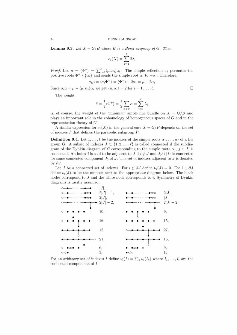
34 DENNIS M. SNOW
Lemma 9.3. Let X = G/B where B is a Borel subgroup of G. Then
c1(X) =∑i=1
2λi
Proof. Let µ = 〈Φ+〉 =∑`
i=1〈µ, αi〉λi. The simple reflection σi permutes thepositive roots Φ+ \ αi and sends the simple root αi to −αi. Therefore,
σiµ = 〈σiΦ+〉 = 〈Φ+〉 − 2αi = µ− 2αi
Since σiµ = µ− 〈µ, αi〉αi we get 〈µ, αi〉 = 2 for i = 1, . . . , `.
The weight
δ =12〈Φ+〉 =
12
∑α>0
α =∑i=1
λi
is, of course, the weight of the “minimal” ample line bundle on X = G/B andplays an important role in the cohomology of homogeneous spaces of G and in therepresentation theory of G.
A similar expression for c1(X) in the general case X = G/P depends on the setof indexes I that defines the parabolic subgroup P .
Definition 9.4. Let 1, . . . , ` be the indexes of the simple roots α1, . . . , α` of a Liegroup G. A subset of indexes J ⊂ 1, 2, . . . , ` is called connected if the subdia-gram of the Dynkin diagram of G corresponding to the simple roots αj , j ∈ J , isconnected. An index i is said to be adjacent to J if i 6∈ J and J0 ∪i is connectedfor some connected component J0 of J . The set of indexes adjacent to J is denotedby ∂J .
Let J be a connected set of indexes. For i 6∈ ∂J define νi(J) = 0. For i ∈ ∂Jdefine νi(J) to be the number next to the appropriate diagram below. The blacknodes correspond to J and the white node corresponds to i. Symmetry of Dynkindiagrams is tacitly assumed.
• · · · • • |J |, • · · · •>• 2|J | − 1, • • · · · •> 2|J |, • · · · •<• 2|J |, • • · · · •< |J |, • · · · • •
•• 2|J | − 2, • • · · · • •
• 2|J | − 2,
• ••
• • 10, • • •
• • 9,
• • ••
• • 16, • • • ••
• 15,
• • • •
• • 12, • • • ••
• • 27,
• • • • ••
• 21, • • • • •
• • 15,
•>• • 6, • •>• 9,<• 3, •< 1,
For an arbitrary set of indexes I define νi(I) =∑
k νi(Ik) where I1, . . . , It are theconnected components of I.
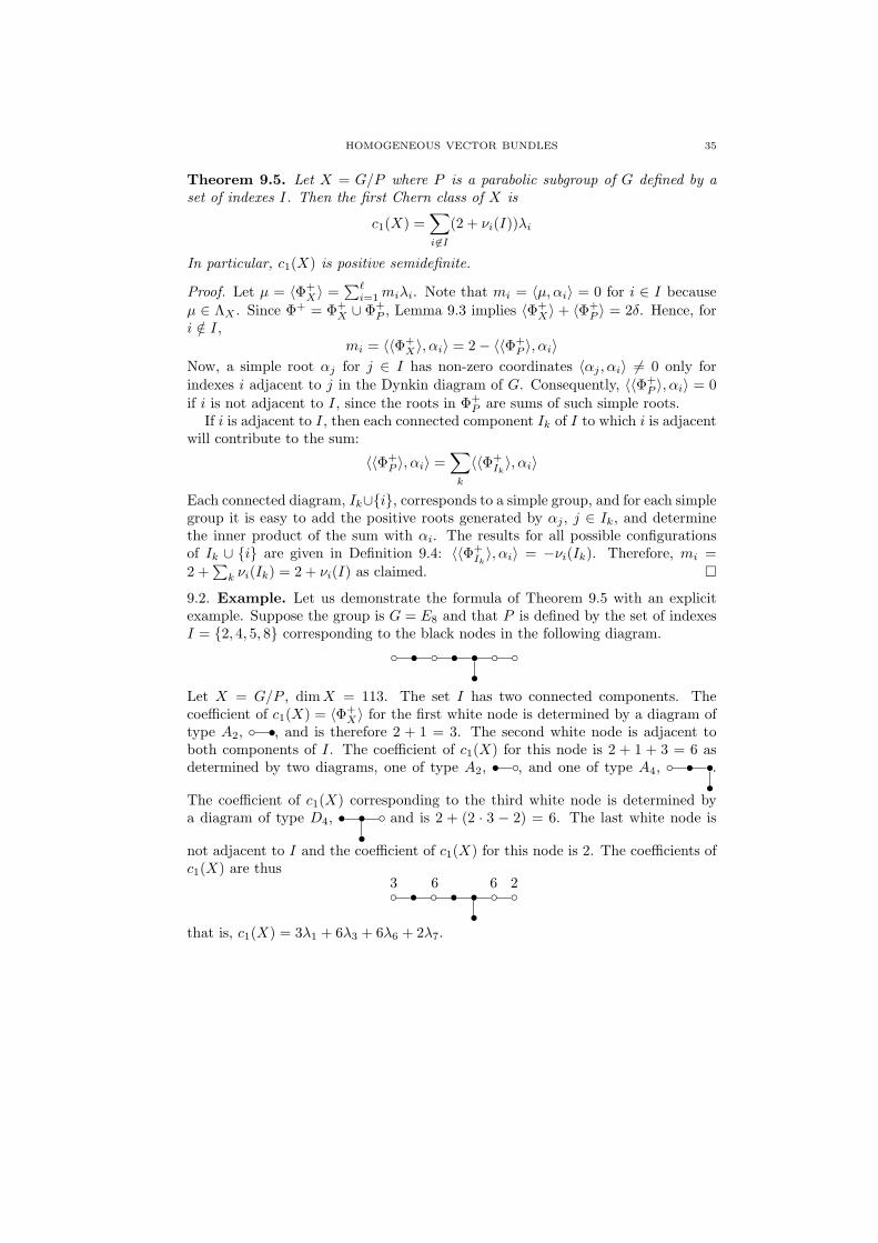
HOMOGENEOUS VECTOR BUNDLES 35
Theorem 9.5. Let X = G/P where P is a parabolic subgroup of G defined by aset of indexes I. Then the first Chern class of X is
c1(X) =∑i 6∈I
(2 + νi(I))λi
In particular, c1(X) is positive semidefinite.
Proof. Let µ = 〈Φ+X〉 =
∑`i=1miλi. Note that mi = 〈µ, αi〉 = 0 for i ∈ I because
µ ∈ ΛX . Since Φ+ = Φ+X ∪ Φ+
P , Lemma 9.3 implies 〈Φ+X〉+ 〈Φ+
P 〉 = 2δ. Hence, fori /∈ I,
mi = 〈〈Φ+X〉, αi〉 = 2− 〈〈Φ+
P 〉, αi〉Now, a simple root αj for j ∈ I has non-zero coordinates 〈αj , αi〉 6= 0 only forindexes i adjacent to j in the Dynkin diagram of G. Consequently, 〈〈Φ+
P 〉, αi〉 = 0if i is not adjacent to I, since the roots in Φ+
P are sums of such simple roots.If i is adjacent to I, then each connected component Ik of I to which i is adjacent
will contribute to the sum:
〈〈Φ+P 〉, αi〉 =
∑k
〈〈Φ+Ik〉, αi〉
Each connected diagram, Ik∪i, corresponds to a simple group, and for each simplegroup it is easy to add the positive roots generated by αj , j ∈ Ik, and determinethe inner product of the sum with αi. The results for all possible configurationsof Ik ∪ i are given in Definition 9.4: 〈〈Φ+
Ik〉, αi〉 = −νi(Ik). Therefore, mi =
2 +∑
k νi(Ik) = 2 + νi(I) as claimed.
9.2. Example. Let us demonstrate the formula of Theorem 9.5 with an explicitexample. Suppose the group is G = E8 and that P is defined by the set of indexesI = 2, 4, 5, 8 corresponding to the black nodes in the following diagram.
• • ••
Let X = G/P , dimX = 113. The set I has two connected components. Thecoefficient of c1(X) = 〈Φ+
X〉 for the first white node is determined by a diagram oftype A2, •, and is therefore 2 + 1 = 3. The second white node is adjacent toboth components of I. The coefficient of c1(X) for this node is 2 + 1 + 3 = 6 asdetermined by two diagrams, one of type A2, • , and one of type A4, • •
•.
The coefficient of c1(X) corresponding to the third white node is determined bya diagram of type D4, • •
• and is 2 + (2 · 3 − 2) = 6. The last white node is
not adjacent to I and the coefficient of c1(X) for this node is 2. The coefficients ofc1(X) are thus
3 6 6 2 • • •
•
that is, c1(X) = 3λ1 + 6λ3 + 6λ6 + 2λ7.
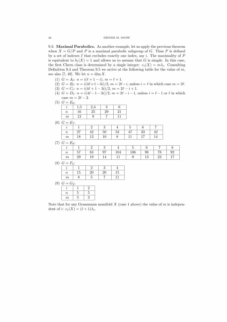
36 DENNIS M. SNOW
9.3. Maximal Parabolics. As another example, let us apply the previous theoremwhen X = G/P and P is a maximal parabolic subgroup of G. Thus P is definedby a set of indexes I that excludes exactly one index, say i. The maximality of Pis equivalent to b1(X) = 1 and allows us to assume that G is simple. In this case,the first Chern class is determined by a single integer: c1(X) = mλi. ConsultingDefinition 9.4 and Theorem 9.5 we arrive at the following table for the value of m,see also [7, 49]. We let n = dimX.
(1) G = A`: n = i(`+ 1− i), m = `+ 1.(2) G = B`: n = i(4`+1−3i)/2, m = 2`− i, unless i = ` in which case m = 2`.(3) G = C`: n = i(4`+ 1− 3i)/2, m = 2`− i+ 1.(4) G = D`: n = i(4`− 1− 3i)/2, m = 2`− i− 1, unless i = `− 1 or ` in which
case m = 2`− 2.(5) G = E6:
i 1,5 2,4 3 6n 16 25 29 21m 12 9 7 11
(6) G = E7:i 1 2 3 4 5 6 7n 27 42 50 53 47 33 42m 18 13 10 8 11 17 14
(7) G = E8:i 1 2 3 4 5 6 7 8n 57 83 97 104 106 98 78 92m 29 19 14 11 9 13 23 17
(8) G = F4:i 1 2 3 4n 15 20 20 15m 8 5 7 11
(9) G = G2:i 1 2n 5 5m 5 3
Note that for any Grassmann manifold X (case 1 above) the value of m is indepen-dent of i: c1(X) = (`+ 1)λi.
HOMOGENEOUS VECTOR BUNDLES 37
10. Nef Value
Let X be a smooth projective variety. A line bundle on X is called numericallyeffective, or nef for short, if its restriction to any effective curve in X yields a linebundle of non-negative degree. If X is homogeneous, it is easy to decide when aline bundle is nef.
Proposition 10.1. Let P be a parabolic subgroup of G and let L be a line bundle onX = G/P defined by a weight λ ∈ ΛX . Then L is nef if and only if λ is dominant.
Proof. Let I be the set of indexes that defines P and write λ =∑
i/∈I niλi. Foreach i /∈ I let Si be the subgroup of G generated by the roots ±αi. Thus, Si
has a Lie algebra isomorphic to sl2(C) and Si ∩ P is a Borel subgroup of Si. Itfollows that the orbit of the identity coset under Si is isomorphic to a rational curve,Ci = Si/Si∩P ∼= P1. Let Li be the line bundle associated to λi for i /∈ I. Then Li|Ci
has degree 1, and since H2(X,Z) ∼= ΛX = ⊕i/∈IZλi it is clear the rational curves Ci,i /∈ I, topologically generate all the curves in X. In particular, if C =
∑i/∈I miCi
is an effective curve, mi ≥ 0 for i /∈ I, then degL|C =∑
i/∈I mini. Consequently,L is nef if and only if ni ≥ 0 for i /∈ I which is the same as λ being dominant.
Note that, by Theorem 6.5, L being nef is equivalent to the a priori strongercondition that L is spanned by global sections.
The canonical bundle of X is defined to be KX =∧n
T ∗X , n = dimX, and is animportant intrinsic line bundle on any projective manifold. For X = G/P , where Pis a parabolic subgroup of G, KX is generated at the identity coset by the exteriorproduct of the duals of Xα, α ∈ Φ+
X , so that the weight associated to KX is
c1(KX) = −∑
α∈Φ+X
α = −∑i 6∈I
(2 + νi(I))λi
The last equality follows from Theorem 9.5; see Definition 9.4 for the meaning ofνi(I). In particular, we see that KX is never nef for a homogeneous manifold X =G/P .
Definition 10.2. Let X be a projective manifold whose canonical bundle KX isnot nef and let L be an ample line bundle on X. The nef value of L, denotedτ(X,L) is defined to be
τ = τ(X,L) = infp/q ∈ Q |KqX ⊗ Lp is nef
The map X → Y ⊂ PN with connected fibers and normal image defined by thesections of some power of Kq
X ⊗ Lp with τ = p/q is called the nef value map of L.
By the Kawamata rationality theorem, τ(X,L) ∈ Q. Moreover, τ(X,L) can becharacterized as the smallest rational number p/q such that Kq
X ⊗Lp is nef but notample, see [2]. For homogeneous manifolds, these facts are easy to deduce. In fact,we have the following formula to calculate τ(X,L), see [49, 50].
Theorem 10.3. Let X = G/P where P is a parabolic subgroup of G defined bya set of indexes I. Let L be an ample line bundle on X with associated weightλ =
∑i 6∈I niλi ∈ Λ+
X . Then
τ(X,L) = maxi 6∈I
2 + νi(I)ni

38 DENNIS M. SNOW
Moreover, the nef value map X → Y is a homogeneous fibration G/P → G/Qwhere Q is defined by the indexes I ∪ J , J = j /∈ I | τ(X,L) = (2 + νj(I))/nj.
Proof. Since L is ample, ni > 0 for all i /∈ I. The weight of KqX ⊗ Lp is∑
i/∈I
(−q(2 + νi(I)) + pni)λi
and this gives a nef but not ample line bundle precisely when the above coeffi-cients are all non-negative and at least one of them is zero, see Theorem 6.5. Thistranslates into
p
q≥ 2 + νi(I)
nifor all i /∈ I
with equality for some i /∈ I. Therefore, τ(X,L) is simply the maximum of (2 +νi(I))/ni, i /∈ I. By construction, the coefficients of the weight µ =
∑miλi
associated to KqX ⊗ Lp with τ(X,L) = p/q satisfy mi = 0 for i ∈ I, mi ≥ 0 for
i /∈ I, and mi = 0 for i /∈ I if and only if (2 + νi(I))/ni = τ(X,L). The map toprojective space defined by the sections of the spanned bundle Kq
X ⊗ Lp is thusthe homogeneous fibration G/P → G/Q where Q = Pµ = PJ as claimed, seeCorollary 6.6.
Corollary 10.4. Let LX be the minimal ample line bundle on X = G/P , i.e., theweight of LX is
∑i 6∈I λi. Then τ(X,LX) = 2 + maxi 6∈I νi(I) ≥ 2. Moreover, for
any ample line bundle L on X, τ(X,L) ≤ τ(X,LX).
Recall that any X = G/P can be decomposed into a product according to thesimple factors of G: X = X1 × · · · × Xt where Xi = Gi/Pi and Pi is a parabolicsubgroup of a simple complex Lie group Gi, i = 1, . . . , t. If L is an ample line bundleon X, then Li = L|Xi
is ample on Xi for all i, and τ(X,L) = maxi τ(Xi, Li). Thisobservation shows that the following proposition is false if G is not assumed to besimple.
Proposition 10.5. Let P be a parabolic subgroup of a simple Lie group G and letLX be the minimal ample line bundle on X = G/P . If π : X → Y is a non-trivialhomogeneous fibration, then τ(X,LX) ≤ τ(Y, LY ) where LY is the minimal ampleline bundle on Y .
Proof. The fibration π is given by a coset map G/P → G/Q, where Q is a parabolicsubgroup of G defined by a set of indexes J ⊃ I. From Definition 9.4, we see thatνi(I) ≤ νi(J) for i 6∈ J . Moreover, Definition 9.4 also shows that for any indexi ∈ J \ I, there is always an index j ∈ ∂J such that νj(J) ≥ νi(I) as long asJ 6= 1, . . . , `. The latter possibility cannot occur, since π is non-trivial. ByCorollary 10.4, τ(X,LX) = 2 + maxi 6∈Iνi(I) ≤ 2 + maxj 6∈Jνj(J) = τ(Y, LY ).
This proposition and the remarks preceding it imply that for a given group Gthe maximum value of τ(X,L) occurs when P is a maximal parabolic subgroupand L = LX is the corresponding minimal ample line bundle on X = G/P . In fact,the nef value in this case is given by the first Chern number, τ(X,LX) = c1(X),see §9.3.
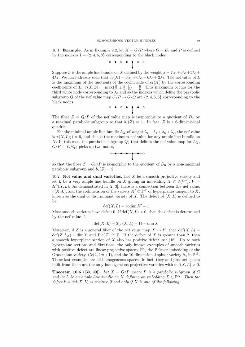
HOMOGENEOUS VECTOR BUNDLES 39
10.1. Example. As in Example 9.2, let X = G/P where G = E8 and P is definedby the indexes I = 2, 4, 5, 8 corresponding to the black nodes
• • ••
Suppose L is the ample line bundle onX defined by the weight λ = 7λ1+6λ3+5λ6+4λ7. We have already seen that c1(X) = 3λ1 +6λ3 +6λ6 +2λ7. The nef value of Lis the maximum of the quotients of the coefficients of c1(X) by the correspondingcoefficients of L: τ(X,L) = max 3
7 , 1,65 ,
12 = 6
5 . This maximum occurs for thethird white node corresponding to λ6 and so the indexes which define the parabolicsubgroup Q of the nef value map G/P → G/Q are 2, 4, 5, 6 corresponding to theblack nodes
• • ••
•
The fiber Z = Q/P of the nef value map is isomorphic to a quotient of D4 bya maximal parabolic subgroup so that b1(Z) = 1. In fact, Z is a 6-dimensionalquadric.
For the minimal ample line bundle LX of weight λ1 +λ3 +λ6 +λ7, the nef valueis τ(X,LX) = 6, and this is the maximum nef value for any ample line bundle onX. In this case, the parabolic subgroup Q0 that defines the nef value map for LX ,G/P → G/Q0 picks up two nodes,
• • • ••
•
so that the fiber Z = Q0/P is isomorphic to the quotient of D6 by a non-maximalparabolic subgroup and b2(Z) = 2.
10.2. Nef value and dual varieties. Let X be a smooth projective variety andlet L be a very ample line bundle on X giving an imbedding X ⊂ P(V ∗), V =H0(X,L). As demonstrated in [2, 3], there is a connection between the nef value,τ(X,L), and the codimension of the variety X ′ ⊂ PN of hyperplanes tangent to X,known as the dual or discriminant variety of X. The defect of (X,L) is defined tobe
def(X,L) = codimX ′ − 1Most smooth varieties have defect 0. If def(X,L) > 0, then the defect is determinedby the nef value [2]:
def(X,L) = 2(τ(X,L)− 1)− dimX
Moreover, if Z is a general fiber of the nef value map X → Y , then def(X,L) =def(Z,LZ) − dimY and Pic(Z) ∼= Z. If the defect of X is greater than 2, thena smooth hyperplane section of X also has positive defect, see [16]. Up to suchhyperplane sections and fibrations, the only known examples of smooth varietieswith positive defect are linear projective spaces, Pn, the Plucker imbedding of theGrassmann variety, Gr(2, 2m+1), and the 10-dimensional spinor variety S4 in P15.These last examples are all homogeneous spaces. In fact, they and product spacesbuilt from them are the only homogeneous projective varieties with def(X,L) > 0.
Theorem 10.6 ([30, 49]). Let X = G/P where P is a parabolic subgroup of Gand let L be an ample line bundle on X defining an imbedding X ⊂ PN . Then thedefect k = def(X,L) is positive if and only if X is one of the following:

40 DENNIS M. SNOW
(1) A linear projective space Pn in PN , k = n.(2) The Plucker imbedding of the Grassmann variety Gr(2, 2m+1) in Pm(2m+1)−1,
k = 2.(3) The 10-dimensional spinor variety S4 in P15, k = 4(4) X1 × X2 where X1 is one of the varieties in 1–3 and defX = defX1 −
dimX2 > 0.
The classification given in [30] is based on invariant theory and proceeds throughmany cases based on the type of the group. The above relationship between thedefect and the nef value, however, can be exploited to give a rather straightforwardclassification which we now sketch.
If X is contained in a hyperplane H then X ′ is a cone over the dual variety ofX ⊂ H with vertex equal to the point dual to H. Conversely, if X ′ is a cone, thenX is contained in the hyperplane dual to the vertex of the cone, see [16]. The defectremains the same whether we consider X as a subvariety of PN or of H ∼= PN−1.Projective space Pn with L = OPn(1) is a special case. Since there are no singularhyperplane sections, the dual variety is empty. In order to be compatible with laterformulas, we adopt the convention that def Pn = n which by the above definitionis the same as assigning the dimension −1 to the empty set.
An important part of the classification of homogeneous spaces with positivedefect involves products: Let X1 and X2 be smooth projective varieties with veryample line bundles L1 and L2, respectively, and dimX1 ≥ dimX2. LetX = X1×X2
and L = pr∗1 L1 ⊗ pr∗2 L2. Then def(X,L) > 0 if and only if def(X1, L1) > dimX2.When this is the case, def(X,L) = def(X1, L1)− dimX2 > 0, see [49, 2].
Now let X = G/P where P is a parabolic subgroup of G and let L be an ampleline bundle on X. Let X = X1×· · ·×Xs be the decomposition of X into irreduciblefactors Xi = Gi/Pi where Gi is simple and Pi ⊂ Gi is parabolic, i = 1, . . . , s. Theabove statements imply that def(X,L) > 0 if and only if def(Xi, Li) > codimX Xi
for some 1 ≤ i ≤ s. In this case
def(X,L) = def(Xi, Li)− codimX Xi > 0
Moreover, the nef value map X → Y associated to L is a homogeneous fibrationG/P → G/Q with fiber Z = Q/P where Q is a parabolic subgroup of G, P is amaximal parabolic subgroup of Q, and
def(X,L) = def(Z,LZ)− dimY
This shows that, up to products and fibrations, it is sufficient to classify homoge-neous spaces X = G/P with positive defect for the case where G is simple and Pis a maximal parabolic subgroup. Other standard facts about dual varieties allowus to assume in addition that L is an ample generator of the line bundles on X,see [17, Theorem 1.3(b)]. Note that when L is such a generator with weight λ, itsdefect is the integer τ given by c1(X) = τλ; see §9.3 for the particular values τcan assume. Using only the numerical criterion that k = 2(τ − 1) > 0 for spaces ofpositive defect k, we arrive at the following list of candidates.
- A`/P1∼= A`/P` (projective space), τ = `+ 1, n = k = `
- A`/P2∼= A`/P`−1 (Grassmann), n = 2(`− 1), τ = `+ 1, k = 2
- A5/P3 (Grassmann), n = 9, τ = 6, k = 1- B`/P1 (quadric), n = τ = 2`− 1, k = 2`− 3- B2/P2 = D4/P4 (projective space), n = 3, τ = 4, k = 3
HOMOGENEOUS VECTOR BUNDLES 41
- B3/P3 = D4/P4 (quadric), n = τ = 6, k = 4- B4/P4 = D5/P5 (spinor), n = 10, τ = 8, k = 4- B5/P5 = D6/P6 (spinor), n = 15, τ = 10, k = 3- B6/P6 = D7/P6 (spinor), n = 21, τ = 12, k = 1- C`/P1, (projective space) n = 2`− 1, τ = 2`, k = 2`− 1- C`/P2, n = 4`− 5, τ = 2`− 1, k = 1- D`/P1 (quadric), n = τ = 2`− 2, k = 2`− 4- E6/P1
∼= E6/P5, n = 16, τ = 12, k = 6- E7/P1, n = 27, τ = 18, k = 7- F4/P4, n = 15, τ = 11, k = 5- G2/P1 (quadric), n = τ = 5, k = 3
The listed value of k is the defect only if the defect is positive, which is not thecase for most of the entries. For example, quadrics are hypersurfaces and obviouslyhave defect 0 (they are self-dual). The fact that A`/P2 = Gr(2, `+ 1) has positivedefect only when ` + 1 is odd has been known for some time [19, 35]. The 10-dimensional spinor variety B4/P4 = D5/P5 is also known to have defect 4, seee.g., [16, 34].
The space C`/P2 is easily seen to have defect 0. Recall that C` = Sp(2`) is thestabilizer of a generic 2-form in
∧2 C2` and stabilizes a (complementary) hyperplanethrough a point of the form [v1∧v2] ∈ P(
∧2 C2`). The isotropy subgroup of [v1∧v2]is conjugate to P2 and therefore C`/P2, which has dimension 4`−5, is a hyperplanesection in Gr(2, 2`). This Grassmann variety has defect 0 as we just pointed out,and so the defect of the hyperplane section C`/P2 must also be 0 by [17, (1.3)].
The exceptional variety E6/P1 cannot have positive defect because its Bettinumbers do not follow the expected pattern for spaces of positive defect k, see [29]:
bn = bn−2, bn−1 = bn−3, · · · , bn−k+1 = bn−k−1
The odd Betti numbers of E6/P1 are zero, and the pertinent even Betti numbersare b16 = 3, b14 = 2, and b12 = 2, see, e.g., [46]. Therefore, the defect of E6/P1 is 0.
The remaining cases are the spaces D6/P6, D7/P7, E7/P1, and F4/P4. Thesespaces do not violate any of the simple criteria for positive defect. They can beshown to have defect 0, however, by computing the fiber dimension (= defect) of theduality map P(N∗
X(1)) → P(V ) where N∗X(1) is the conormal bundle of X ⊂ PN
twisted by OX(1). This calculation can be reduced to determining the rank ofmatrix involving certain roots and structure constants, see [49].
At this point we can conclude that the only homogeneous spaces G/P , P max-imal, having an ample line bundle with positive defect are the familiar examples:Pk, Gr(2, 2m+ 1) or S4. The general case is handled as follows.
Suppose X = G/P and L is a minimal ample line bundle on X with def(X,L) >0. Since the case of products has already been discussed above, we may assume thatG is simple. The nef value map X = G/P → Y = G/Q has fiber Z = Q/P whereP is a maximal parabolic subgroup of Q. Since def(X,L) = def(Z,LZ)− dimY >0 implies def(Z,LZ) > 0, the only possibilities for Z are the three spaces justmentioned. If Z = Gr(2, 2m + 1) then def(Z,LZ) = 2 forcing dimY < 2. IfdimY = 1 then Y ∼= P1, and G = SL(2,C) which is too small to provide a non-trivial fibration. Thus, dimY = 0 andX = Z. Similarly, if Z = S4, then dimY < 4.The limited possibilities for Y imply that G is of type Ar, r = 1, 2, 3 or B2. Noneof these can contain either of the two simple Lie groups that act transitively on the
42 DENNIS M. SNOW
10-dimensional spinor variety S4 (B4 or D5). So again we deduce that the fibrationis trivial and X = Z. The final possibility of a non-trivial fibration with Z = Pk
can be ruled out since for any such fibration one must have dimY > k and thiscontradicts def(Z,LZ)− dimY > 0, see [49, 4.1]. This concludes the sketch of theproof of Theorem 10.6.
The following statement holds for non-linear smooth projective varieties X ⊂ PN
such that dimX = dimX ′ ≤ 23N , see [16]. The version we present here for homoge-
neous spaces is simply a corollary of the previous classification. This list also clas-sifies those non-linear homogeneous spaces with non-singular dual varieties, since anon-singular dual implies that dimX = dimX ′, see [16]. If X is a linear projectivespace, X = Pn ⊂ PN , then the tangent hyperplanes are clearly parameterized by acomplementary projective space X ′ = PN−n−1.
Corollary 10.7. Let X = G/P be a non-linear homogeneous space imbedded inPN by the sections of an ample line bundle L on X. If dimX = dimX ′ then X isone of the following:
(1) A quadric hypersurface in Pn+1
(2) The Segre imbedding of Pn−1 × P1 in P2n−1
(3) The Plucker imbedding of Gr(2, 5) in P9
(4) The 10-dimensional spinor variety S4 in P15
Proof. The listed varieties are well-known to be self-dual, see e.g., [16, 19, 34]. IfX = Gr(2, 2m + 1) then dimX = 2(2m − 1) and dimX ′ = m(2m + 1) − 4 andthese are equal only when m = 2. By Theorem 10.6 it remains to check the caseX = X1 × X2. Since L = pr∗1 L1 ⊗ pr∗2 L2 and hence H0(X,L) ∼= H0(X1, L1) ⊗H0(X2, L2), the imbedding dimension of X satisfies N+1 = (N1+1)(N2+1) whereNi is the imbedding dimension of Xi under Li, i = 1, 2. We know that defX =N −dimX− 1 = defX1−dimX2. Hence, N1N2 +N1 +N2 = dimX1 +defX1 +1.Since Ni ≥ dimXi this equation becomes dimX2(dimX1 + 1) ≤ defX1 + 1. Now,X1 must be a projective space, for otherwise defX1 + 1 ≤ 5 and this would implythat dimX1 = 1. Therefore, (X1, L1) ∼= (Pn1 ,OPn1 (1)) and the previous equationyields N2 = 1. This implies that (X2, L2) = (P1,OP1(1)), and X = Pn−1 × P1 asclaimed.
Certain real hypersurfaces in complex projective space are tubes over complexsubmanifolds, see [12]. This fact along with the above classification of self-dualhomogeneous spaces can be used to classify homogeneous real hypersurfaces incomplex projective space.
Corollary 10.8 ([57]). Let M be a homogeneous complete real hypersurface imbed-ded equivariantly in PN . Then M is a tube over a linear projective space or one ofthe 4 self-dual homogeneous spaces X ⊂ PN listed in Corollary 10.7.
Proof. Let M = K/L where K is a compact Lie group and let ξ denote the normalvector field to M . If J denotes the complex structure operator, then W = −Jξ is atangent vector field. Because the imbedding is equivariant, W is left invariant underK and therefore its integral curves are given by 1-parameter subgroups of K andare geodesics. By [12], M is a tube over a complex submanifold X ⊂ PN (a focalsubmanifold). In particular, X is homogeneous, X = G/P , and G acts transitivelyon the normal directions toX. It follows that the conormal variety P(N∗
X(1)) itself isa homogeneous space, G/P0, and therefore the image of P(N∗
X(1)) = G/P0 −→ X ′
HOMOGENEOUS VECTOR BUNDLES 43
must also be homogeneous, X ′ = G/P ′. If X is not a linear projective spacethen dimX ′ = dimX, and so X is one of 4 self-dual homogenoeus spaces byCorollary 10.7.
Conversely, the classification of homogeneous real hypersurfaces [57] can also beused to obtain the list of self-dual homogeneous spaces. For, if a homogeneousspace X = G/P is self-dual, then by a symmetry argument, the conormal varietymust be a homogeneous space under G. This implies that G acts transitively on thenormal directions to X and hence a maximal compact subgroup of G must have ahypersurface orbit in the normal bundle of X. The resulting orbit is a homogeneousreal hypersurface in PN realized as a tube over X and therefore must be on the listgiven in [57].
44 DENNIS M. SNOW
11. Cohomology
Let E = G ×P E0 be a homogeneous vector bundle on X = G/P where P isa parabolic subgroup of G. We denote by Hq(X,E) the q-th Cech cohomologywith coefficients in the sheaf of local holomorphic sections of E. In [9], Bott givesa precise way to compute these cohomology groups in the case where the repre-sentation of P on E0 is irreducible. Subsequently other proofs have been found,see, e.g., [31, 15]. We shall now sketch the proof of Bott’s theorem and give someapplications.
Recall from §9.1 that the weight δ ∈ Λ+ is defined by
δ =∑i=1
λi =12
∑α>0
α
so that 〈δ, α〉 = 1 and σα(δ) = δ − α for any simple root α. Recall also that thedominant conjugate of a weight λ ∈ Λ is denoted by [λ] ∈ Λ+, see §3.
The proof of Bott’s theorem relies on Serre Duality and an application of Leray’sspectral sequence. Serre duality states that for a holomorphic vector bundle E ona compact complex manifold X of dimension n,
Hq(X,E) ∼= Hn−q(X,KX ⊗ E)∗
where KX =∧n
T ∗X is the canonical bundle of X, see [43]. The version of Leray’sspectral sequence we need is the following, see [25, Theoreme 4.17.1].
Lemma 11.1. Let π : Y → X be a locally trivial holomorphic fibration with aconnected compact fiber Z and let F be a holomorphic vector bundle on Y . Thereis a spectral sequence Er with
Eq,p2 = Hq(X,Hp(Z,FZ))
whose final term is associated to H∗(Y, F ). In particular, if Hp(Z,FZ) = 0 exceptfor p = k, then the spectral sequence is trivial and therefore
Hq(Y, F ) ∼= Hq−k(X,Hk(Z,FZ))
for all q ≥ 0
Using this spectral sequence, Bott’s theorem can be easily reduced to the caseof line bundles on G/B, a case we must handle first.
Proposition 11.2. Let B be a Borel subgroup of G and let L be a holomorphicline bundle on Y = G/B. Let λ ∈ Λ be the weight associated to L.
(1) If λ+ δ is singular, then Hq(Y, L) = 0 for all q.(2) If λ + δ is not singular, then Hq(Y, L) = 0 for all q 6= ind(λ + δ), and for
q = ind(λ + δ), Hq(Y, L) is isomorphic to the irreducible G-module withhighest weight [λ+ δ]− δ.
Proof. We first make some general observations. Let α be a simple root and letPα be the minimal parabolic subgroup defined by α. Consider the fibration Y =G/B → Yα = G/Pα with fiber Zα = Pα/B ∼= P1. Let Kα be the canonical bundleof Zα, so the weight associated to Kα is −α.
If 〈λ + δ, α〉 ≤ 0 then 〈λ, α〉 ≤ −1. This implies that H0(Zα, L) = 0 by Theo-rem 6.5. Applying Lemma 11.1 we see that for q ≥ 0,
Hq(Y, L) ∼= Hq−1(Yα,H1(Zα, L))
HOMOGENEOUS VECTOR BUNDLES 45
By Serre duality,H1(Zα, L) ∼= H0(Zα,Kα ⊗ L−1)∗
The weight of the line bundle Kα ⊗ L−1 is −λ− α. We consider the two cases:(i) If 〈λ+ δ, α〉 = 0 then 〈−λ−α, α〉 = −1 and hence H0(Zα,Kα⊗L−1) = 0 by
Theorem 6.5. Therefore, Hq(Y,L) = 0 for all q ≥ 0.(ii) If 〈λ+δ, α〉 < 0 then 〈−λ−α, α〉 ≥ 0 so that H0(Zα,Kα⊗L−1) is isomorphic
to the irreducible Pα-module with maximal weight −λ − α by Theorem 6.5. Thedual of this module has maximal weight
−σα(−λ− α) = σα(λ)− α = σα(λ+ δ)− δ
see §4. Let σαL denote the line bundle defined by the weight σα(λ+ δ)− δ. Then,for all q,
Hq(Y, L) ∼= Hq−1(Yα,H0(Zα,Kα ⊗ L−1)∗)
∼= Hq−1(Yα,H0(Zα, σαL))
∼= Hq−1(Y, σαL)
The last isomorphism follows from Lemma 11.1 again because H1(Zα, σαL) van-ishes: by Serre Duality, H1(Zα, σαL) ∼= H0(Zα,Kα⊗σαL
−1)∗ and the latter groupis zero by Theorem 6.5 since 〈−σα(λ+ δ) + δ − α, α〉 = 〈λ, α〉 < 0.
To prove the theorem, let αi(1), . . . , αi(t) denote a sequence of simple roots suchthat 〈λ+δ, αi(1)〉 < 0, 〈σi(1)(λ+δ), αi(2)〉 < 0,. . . , 〈σi(t−1) · · ·σi(1)(λ+δ), αi(t)〉 < 0,and 〈σi(t) · · ·σi(1)(λ+ δ), α〉 ≥ 0 for all simple roots α. Then t = ind(λ+ δ) and thedominant conjugate of λ + δ is [λ + δ] = σ(λ + δ) where σ = σi(t) · · ·σi(1), see §3.Therefore, repeatedly applying the above isomorphism gives
Hq(Y, L) ∼= Hq−1(Y, σi(1)L) ∼= Hq−2(Y, σi(2)σi(1)L) ∼= · · · ∼= Hq−t(Y, σL)
The weight associated to σL is [λ+ δ]− δ. This shows that Hq(Y,L) = 0 for q < t.If 〈[λ + δ], α〉 = 0 for some simple root α—this is equivalent to λ + δ being
singular—then the spectral sequence argument of (i) above shows thatHq(Y, σL) =0 for all q ≥ 0 so that Hq(Y,L) = 0 for all q ≥ 0. If 〈[λ + δ], α〉 6= 0 for all simpleroots α, then [λ+δ]−δ is dominant and hence Ht(Y,L) = H0(Y, σL) is isomorphicto the irreducible G-module with highest weight [λ+ δ]− δ by Theorem 6.5. To seethat Hq(Y,L) = 0 for q > t, apply Serre duality:
Hq−t(Y, σL) ∼= Hn−q+t(Y,KY ⊗ σL−1)∗
where n = dimY . The weight of KY ⊗ σL−1 is µ = −[λ + δ] − δ since the weightof KY is −2δ, see §9. Now, because [λ + δ] is non-singular and dominant, thedominant conjugate of µ + δ = −[λ + δ] is [µ + δ] = −ω0[λ + δ] where ω0 is thelongest element in the Weyl group, `(ω0) = ind(µ+ δ) = n, see §3. Thus, by whatwe have just proved,
Hn−q+t(Y,KY ⊗ σL−1) ∼= Ht−q(Y, τL)
where τL is the line bundle on Y associated to the weight [µ + δ] − δ. Therefore,Hq(Y, L) = 0 for q > t as well. Note that the dual of the G-module H0(Y, τL) isH0(Y, σL) since −ω0([µ+ δ]− δ) = [λ+ δ]− δ, see §4.
Theorem 11.3 (Bott). Let E = G ×P E0 be a homogeneous holomorphic vectorbundle on X = G/P where P is a parabolic subgroup of G. Assume E0 is anirreducible representation of P with maximal weight λ ∈ ΛX . Let B be a Borel
46 DENNIS M. SNOW
subgroup of G and let L = G ×B C be the line bundle on Y = G/B associated tothe weight λ. Then, for all q
Hq(X,E) ∼= Hq(Y, L)
In particular,(1) If λ+ δ is singular, then Hq(X,E) = 0 for all q.(2) If λ+ δ is not singular, then Hq(X,E) = 0 for all q 6= ind(λ+ δ), and for
q = ind(λ + δ), Hq(X,E) is isomorphic to the irreducible G-module withhighest weight [λ+ δ]− δ.
Proof. Consider the equivariant fibration Y = G/B → X = G/P with fiber Z =P/B. Since λ is P -dominant, Proposition 11.2 implies thatH0(Z,LZ) is isomorphicto the irreducible representation of P with maximal weight λ, and Hq(Z,LZ) = 0for q > 0. Therefore, π∗L ∼= E and by Lemma 11.1,
Hq(Y, L) ∼= Hq(X,H0(Z,LZ)) = Hq(X,E)
The last assertions then follow from Proposition 11.2 applied to L.
Bott’s original proof used the Kodaira vanishing theorem, but this can be avoidedby applying Serre duality and exploiting the two-fold symmetry in the Weyl groupas in the proof of Proposition 11.2. This approach also allows a purely algebraicproof of Bott’s theorem, see [15]. The above proof retains the spirit of of Bott’sargument which shows how weights of the form σ(λ + δ) − δ appear due to SerreDuality.
Bott’s theorem allows us to calculate the cohomology a homogeneous vectorbundle that is the direct sum of irreducible homogeneous bundles, E = m1F1 ⊕· · · ⊕ mtFt, with multiplicities mi and maximal weights µi, 1 ≤ i ≤ t. If M(q)denotes the subset of these weights µi such that ind(µi + δ) = q and µi + δ isnon-singular, 1 ≤ i ≤ t, then
Hq(X,E) ∼=⊕
µi∈M(q)
miV[µi+δ]−δ
and the G-module structure of Hq(X,E) is completely determined. In particular,the dimension of Hq(X,E) can calculated using Weyl’s dimension formula, see §4.We shall see an example of this later: on a compact hermitian symmetric space thebundle of holomorphic p-forms, Ωp
X , is a direct sum of irreducible vector bundlesof known maximal weights. The cohomology of Ωp
X ⊗Lk can then be computed asjust described for any line bundle L on X.
Of course, many homogeneous vector bundles of interest are not direct sumsof irreducible homogeneous vector bundles. Nevertheless, using filtrations, Bott’stheorem can often be applied indirectly to predict when certain cohomology groupsvanish, cf. [21].
Proposition 11.4. Let E = G ×P E0 be a homogeneous vector bundle on X =G/P where P is a parabolic subgroup of G. Let M(E0) denote the set of indexes,ind(µ+ δ), for all maximal weights µ ∈ Λmax(E0) such that µ+ δ is non-singular.Then Hq(X,E) = 0, if q 6∈M(E0).
Proof. Let E0 ⊃ E1 ⊃ · · · ⊃ Et ⊃ Et+1 = 0 be a filtration of E0 by P -submoduleswith irreducible subquotients Fi = Ei/Ei+1 of maximal weights µi, i = 0, . . . , t.
HOMOGENEOUS VECTOR BUNDLES 47
The short exact sequences 0 → Ei+1 → Ei → Fi → 0, i = 0, . . . , t, lead to thefollowing long exact sequences
. . . → Hq(X,Ft) → Hq(X,Et−1) → Hq(X,Ft−1) → . . .
. . . → Hq(X,Et−1) → Hq(X,Et−2) → Hq(X,Ft−2) → . . .· · ·
. . . → Hq(X,E1) → Hq(X,E) → Hq(X,F0) → . . .
Bott’s Theorem 11.3 implies that Hq(X,Fi) = 0 if q 6= ind(µi + δ) or if µi + δ issingular, 0 ≤ i ≤ t. Therefore, if q 6∈M(E0), thenHq(X,Et−1) = 0,Hq(X,Et−2) =0, . . ., Hq(X,E) = 0.
In the special case when M(E0) = 0 a stronger statement holds which can beviewed as a generalization of the Borel-Weil Theorem 6.5 to vector bundles.
Corollary 11.5. Let E = G×P E0 be a homogeneous vector bundle on X = G/Pwhere P is a parabolic subgroup of G. If the maximal weights of E0 are dominant,Λmax(E0) ⊂ Λ+, then E is generated by global sections and Hq(X,E) = 0 for q > 0.
Proof. As in Propostition 11.4 we have Hq(X,E) = 0 for q > 0 and H0(X,E) ∼=⊕iH
0(X,Fi). Moreover, since the µi are dominant, the evaluation maps X ×H0(X,Fi) → Fi are surjective. Therefore, by universality of induced modules, seeProposition 5.1, the evaluation map X × H0(X,E) → E is surjective and E isgenerated by global sections.
A version of the this theorem for Dolbeault cohomology will be presented in § ??.
11.1. Tangent Bundles and Rigidity. One of the applications of Bott’s theoremgiven in his original paper [9] is to show that the complex structure on X = G/Pcannot be locally deformed. This result relies on Kodaira-Spencer theory, see [32],which says that if Xt is a smooth deformation of the complex structure of X = X0
and if H1(X,TX) = 0, then Xt is holomorphically isomorphic to X for all t near 0.Recall that the tangent bundle on X = G/P is naturally a homogeneous vector
bundle. The representation of P on the the tangent space at the identity coset isisomorphic to the P -module g/p with the induced adjoint action, see §2. The exactsequence of P -modules
0 −→ p −→ g −→ g/p −→ 0
thus induces a corresponding exact sequence of vector bundles on X
0 −→ F −→ E −→ TX −→ 0
Since the adjoint representation of P on g extends to the adjoint representation ofG on g, the bundle E is trivial and hence Hq(X,E) = 0 for q ≥ 1, see §5. Therefore,from the associated long exact sequence we obtain
Hq(X,TX) ∼= Hq+1(X,F ) q ≥ 1
The weights of F = G×P p are all the negative roots of G, 0, and all the positiveroots of P . To apply Proposition 11.4 we need to know the index of non-singularweights of the form α+ δ for all such roots α.
This calculation is not hard to carry out explicitly. The general result is thatfor any root α ∈ Φ, if α + δ is non-singular then ind(α + δ) ≤ 1. For example, ifall roots have the same length (i.e., G is composed of types A`, D` or E`) then thecoordinates of any root in the basis of fundamental dominant weights are always 0,

48 DENNIS M. SNOW
+1, or −1, except for the simple roots whose coordinates are given by the rows ofthe Cartan matrix. Since δ has all coordinates equal to 1, it is clear that α + δ iseither singular (a coordinate is 0) or has index 0 (all coordinates positive), unless−α is a simple root. When −α is simple, δ+α = σ−α(δ) and so δ+α has index 1.Similar arguments can be worked out for the other types; a detailed proof can befound in [9, p.220].
We conclude from Proposition 11.4 thatHq(X,F ) = 0 for q ≥ 2 which establishesthe following proposition and corollary.
Proposition 11.6. Let X = G/P where P is a parabolic subgroup of G. ThenHq(X,TX) = 0 for q ≥ 1.
Corollary 11.7. The complex structure of X = G/P is locally rigid.
11.2. Line Bundles. Since every holomorphic line bundle L on X = G/P is ho-mogeneous and is thus defined by an irreducible 1-dimensional representation ofP , i.e., by a weight λ ∈ ΛX , Bott’s theorem applies particularly well to this case.If λ + δ is singular, then all the cohomology groups Hq(X,L) vanish. Otherwise,precisely one cohomology group is non-zero in degree ind(λ+ δ), and this group isisomorphic to the irreducible G-module V [λ+δ]−δ.
We would now like to relate Bott’s theorem for line bundles to the vanishingtheorem proved in §7.3 based on the curvature of L. Recall Theorem 7.6 states thatthe number of positive eigenvalues of the Levi form, L(φL), of a tube neighborhoodof the zero section in L is given by ind(λ) and the number of negative eigenvaluesby ind(−λ). The theorem of Andreotti-Grauert then implies that for sufficientlylarge m, Hq(X,Lm) = 0 if q < ind(λ) or q > dimX − ind(−λ). Moreover, if λ isnon-singular, then ind(λ) + ind(−λ) = dimX and Hq(X,Lm) = 0 for q 6= ind(λ).
The weight of Lm is mλ and it is interesting to observe that for sufficiently largem, both mλ and mλ+ δ must lie in the same Weyl chamber. We need only choosem large enough so that if 〈α,mλ〉 < 0 then 〈α,mλ〉 < −1 for all positive rootsα > 0. Notice that this also guarantees that mλ+ δ is non-singular. Thus,
ind(mλ+ δ) = ind(mλ) = ind(λ)
By Bott’s theorem, Hq(X,Lm) = 0 for q 6= ind(λ) and Hq(X,Lm) ∼= V [mλ+δ]−δ
when q = ind(λ).
HOMOGENEOUS VECTOR BUNDLES 49
References
[1] Andreotti, A., Grauert, H. Theoremes de finitude pour la cohomologie des espaces complexes,Bull. Math. Soc. France 90 (1962), 193–259.
[2] Beltrametti, M., Fania, M., Sommese, A., On the discriminant variety of a projective mani-
fold, Forum Math. 4 (1992), 529–547.[3] Beltrametti, M., Sommese, A., Wisniewski, J., Results on varieties with many lines and
their applications to adjunction theory, Lecture Notes in Math., vol. 1507, Springer, Berlin,
Heidelberg, New York, 1992.[4] Borel, A., Linear Algebraic Groups, 2nd ed., Benjamin, New York, 1991.
[5] Borel, A., A spectral sequence for complex analytic bundles, in Hirzebruch, F., TopologicalMethods in Algebraic Geometry, 3rd Edition, Springer, Berlin, Heidelberg, New York, 1978.
[6] Borel, A., Topology of Lie groups and characteristic classes, Bull. Amer. Math. Soc. 61
(1955), 397–432.
[7] Borel, A., Hirzebruch, F., Characteristic classes and homogeneous spaces, part I, Amer. J.Math. 80 (1958), 459–538.
[8] Borel, A., Hirzebruch, F., Characteristic classes and homogeneous spaces, part II, Amer. J.Math. 81 (1959), 315–381.
[9] Bott, R., Homogeneous vector bundles, Ann. Math. 66 (1957), 203–248.
[10] Bourbaki, N., Groupes et algebres de Lie, Chapt. 4–6, Hermann, Paris, 1960.[11] Cline, E., Parshall B., Scott L., Induced modules and affine quotients, Math. Ann. 230 (1974),
1–14.
[12] Cecil, T., Ryan, P., Focal sets and real hypersurfaces in complex projective space, Trans.Amer. Math. Soc. 269 (1982), 481-499.
[13] Deligne, P., Dimca, A., Filtrations de Hodge et par l’ordre du pole pour les hypersurfaces
singulieres, Ann. Sci. Ecole Norm. Sup. (4) 23 (1990), 645–656.[14] Demailly, J.P., Vanishing theorems for tensor powers of an ample vector bundle, Invent.
Math. 91 (1988), 203–220.
[15] Demazure, M., A very simple proof of Bott’s theorem, Invent. Math. 33 (1976), 271–272.[16] Ein, L., Varieties with small dual varieties, I, Invent. Math. 86 (1986), 63–74.
[17] Ein, L., Varieties with small dual varieties, II, Duke Math. J. 52 (1985), 895–907.[18] Faltings, G., Formale Geometrie and homogene Raume, Invent. Math. 64 (1981), 123–165.
[19] Griffiths, P., Harris, J., Algebraic geometry and local differential geometry, Ann. Sci. EcoleNorm. Sup. 12 (1979), 355–432.
[20] Griffiths, P., Harris, J., Principles of Algebraic Geometry, Wiley, New York, 1978.
[21] Griffiths, P., Some geometric and analytic properties of homogeneous complex manifolds, I,Acta Math. 110 (1963), 115–155.
[22] Griffiths, P., On the differential geometry of homogeneous vector bundles, Trans. Amer. Math.
Soc. 109 (1963), 1–34.[23] Griffiths, P., Hermitian differential geometry, Chern classes, and positive vector bundles, in
D. Spencer, S. Iyanaga, ed., Global Analysis, Univ. of Tokyo Press, Princeton Univ. Press
(1969), 185–251[24] Griffiths, P., Schmid, W. Locally homogeneous manifolds, Acta Math. 123 (1970), 253–302.
[25] Godemont, R., Topologie algebrique et theorie des faisceaux, Hermann, Paris, 1958.[26] Goldstein, N., Ampleness and connectedness in complex G/P , Trans. Amer. Math. Soc. 274
(1982), 361–373.
[27] Humphreys, J. Introduction to Lie Algebras and Representation Theory, Springer, Berlin,Heidelberg, New York, 1972.
[28] Jacobson, N. Lie Algebras, Wiley & Sons, New York, 1962.
[29] Kleiman, S., Tangency and Duality, CMS Conf. Proc. 6 (1986), 164–225.[30] Knop, F., Menzel, G., Dualen Varietaten von Fahnenvarietaten, Comment. Math. Helvetici
62 (1987), 38–61.
[31] Kostant, B., Lie algebra cohomology and the generalized Borel Weil Theorem, Ann. Math.74 (1961), 329–387.
[32] Kodaira, K., Spencer, D., On deformations of complex analytic structures, Ann. Math. 67
(1958), 328–466.[33] Lanteri, A., Struppa, D., Projective 7-folds with positive defect, Compositio Math. 61 (1987),
329–337.
50 DENNIS M. SNOW
[34] Lazarsfeld, R., Van de Ven, A., Topics in the Geometry of Projective Space, Recent Work ofF.L. Zak, Birkhauser, Basel, Boston, Stuttgart, 1984.
[35] Lascoux, A., Degree of the dual of a Grassmann variety, Comm. in Alg. 9 (1981), 1215–1225.
[36] Le Potier, J., Annulation de la cohomologie a valeurs dans un fibre vectoriel holomorphepositif de rang quelconque, Math. Ann. 218 (1975), 35–53.
[37] Le Potier, J., Cohomologie de la Grassmannienne a valeurs dans les puissances exterieurs etsymmetriques du fibre universel, Math. Ann. 226 (1977), 257–270.
[38] Manivel, L., Un theoremes d’annulation pour les puissances exterieures d’un fibre ample, J.
reine angew. Math. 422 (1991), 91–116.[39] Manivel, L., Theoremes d’annulation pour les fibres associes a un fibre ample, Scuola Norm.
Sup. Pisa 19 (1992), 515–565.
[40] Mori, S., Projective manifolds with ample tangent bundle, Ann. Math. 110 (1979), 593–606.[41] Moody, R., Patera, J., Fast recursion formula for weight multiplicities, Bull. Amer. Math.
Soc. 7 (1982) 237–242.
[42] Serre, J.P., Repreesentations lineares et espaces homogenes Kahlerians des groupes de Liecompacts (d’ares Borel et Weil), Sem. Bourbaki, Expose 100, May 1954, Benjamin, New
York, 1966.
[43] Serre, J.-P., Un theoreme de dualite, Comment. Math. Helv. 29 (1955), 9–25.[44] Snow, D. M., On the ampleness of homogeneous vector bundles, Trans. Amer. Math. Soc.
294 (1986), 585–594.[45] Snow, D. M., Cohomology of twisted holomorphic forms on Grassmann manifolds and quadric
hypersurfaces, Math. Ann. 276 (1986), 159–176.
[46] Snow, D. M., Vanishing theorems on compact hermitian symmetric spaces, Math. Z. 198(1988), 1–20.
[47] Snow, D. M., Weyl group orbits, A.C.M. Trans. Math. Software 16 (1990), 94–108.
[48] Snow, D. M., Computing Tensor Product Decompositions, Trans. Math. Software 19 (1993),95–108.
[49] Snow, D. M., The nef value and defect of homogeneous line bundles, Trans. Amer. Math.
Soc. 340 (1993), 227–241.[50] Snow, D. M., The nef value of homogeneous line bundles and related vanishing theorems, to
appear Forum Math.
[51] Snow, D. M., Weller, K., A vanishing theorem for generalized flag manifolds, to appearArchiv. Math.
[52] Manivel, L., Snow, D. M., A Borel-Weil theorem for holomorphic forms, preprint.[53] Sommese, A., Submanifolds of abelian varieties, Math. Ann. 233 (1978), 229–256.
[54] Sommese, A., A convexity theorem, Proc. Sympos. Pure Math. 40 (1983), 497–405.
[55] Sommese, A., Complex subspaces of homogeneous complex manifolds, I, Duke Math. J.46(1979), 527–548.
[56] Sommese, A., Complex subspaces of homogeneous complex manifolds, II, Nagoya Math. J.86
(1982), 101–129.[57] Takagi, R., On homogeneous real hypersurfaces in a complex projective space, Osaka J. Math.
10 (1973), 495–506.
[58] Tits, J., Tabellen zu den Einfachen Lie Gruppen und ihren Darstellungen, Lecture Notes inMath., vol. 40, Springer, Berlin, Heidelberg, New York, 1967.
[59] Weyl, H., Theorie der Darstellun der halb-einfacher Gruppen durch lineare Transformationen,
Math. Z. 24 (1926), 377–395.
HOMOGENEOUS VECTOR BUNDLES 51
Department of Mathematics, University of Notre Dame, Notre Dame, IN 46556


![Weyl points in photonic-crystal superlatticessoljacic/Weyl-points_2DMat.pdf · of Weyl points have been reported in a three-dimensional double-gyroid photonic crystal [45] and in](https://img.pdfslide.net/doc/110x75/5ec846dbd0cd7c3a730fb4cc/weyl-points-in-photonic-crystal-soljacicweyl-points2dmatpdf-of-weyl-points.jpg)

![AParametricFamilyofSubalgebrasoftheWeylAlgebra I ... · Quantum planes and quantum Weyl algebras are generalized Weyl algebras in the sense of [B, 1.1] and their structure and irreducible](https://img.pdfslide.net/doc/110x75/5f3af586e1521f0b57282eb6/aparametricfamilyofsubalgebrasoftheweylalgebra-i-quantum-planes-and-quantum.jpg)

![PART I: SYMPLECTIC ICE. PART II: GLOBAL AND …sd054cv7359/...Hamel and King [7] showed how characters of irreducible representations times the deformed Weyl denominators are equal](https://img.pdfslide.net/doc/110x75/5ed71a66a524404e761742e9/part-i-symplectic-ice-part-ii-global-and-sd054cv7359-hamel-and-king-7-showed.jpg)