Motivation Background Continuous Count Queries on WSNs Performance Evaluation Conclusion

2

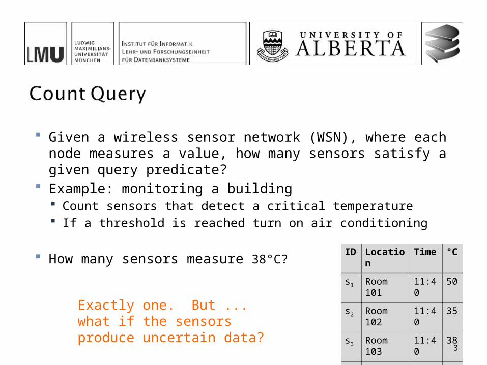
Given a wireless sensor network (WSN), where each node measures a value, how many sensors satisfy a given query predicate?

Example: monitoring a building Count sensors that detect a critical temperature If a threshold is reached turn on air conditioning

ID Location Time °C

s1 Room 101 11:40 50

s2 Room 102 11:40 35

s3 Room 103 11:40 38

s4 Room 203 11:40 40

... ... ... ...3

How many sensors measure 38°C?

Exactly one. But ... what if the sensors produce uncertain data?

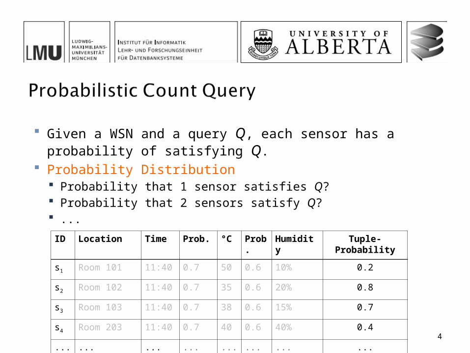
Given a WSN and a query Q, each sensor has a probability of satisfying Q.

Probability Distribution Probability that 1 sensor satisfies Q? Probability that 2 sensors satisfy Q? ...

ID Location Time Prob. °C Prob. Humidity Tuple-Probability

s1 Room 101 11:40 0.7 50 0.6 10% 0.2

s2 Room 102 11:40 0.7 35 0.6 20% 0.8

s3 Room 103 11:40 0.7 38 0.6 15% 0.7

s4 Room 203 11:40 0.7 40 0.6 40% 0.4

... ... ... ... ... ... ... ... 4

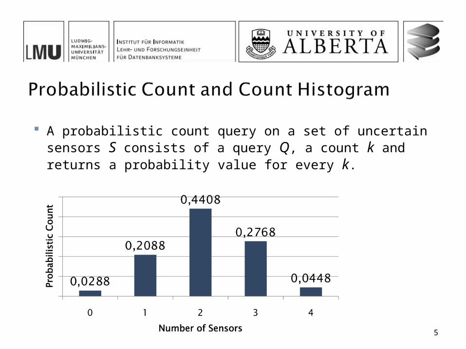
A probabilistic count query on a set of uncertain sensors S consists of a query Q, a count k and returns a probability value for every k.

5

Exactly k sensors in a set of sensors S satisfy Q only if sensor sx in S satisfies Q and k-1 other sensors in S satisfy Q or

sensor sx in S doesn‘t satisfy Q and k other sensors in S satisfy Q

Each probability value is an independent Bernoulli random variable with

Possible World Wk,j Probability P(Wk,j)

W4,1 = {s1,s2,s3, s4} 0.2*0.8*0.7*0.4=0.0448

W3,1 = {s1,s2,s3} 0.2*0.8*0.7*(1-0.4)=0.0672

W3,2 = {s1,s2, s4} 0.2*0.8*(1-0.7)*0.4=0.0192

... ...

W0,1 = {} (1-0.2)*(1-0.8)*(1-0.7)*(1-0.4)=0.0288

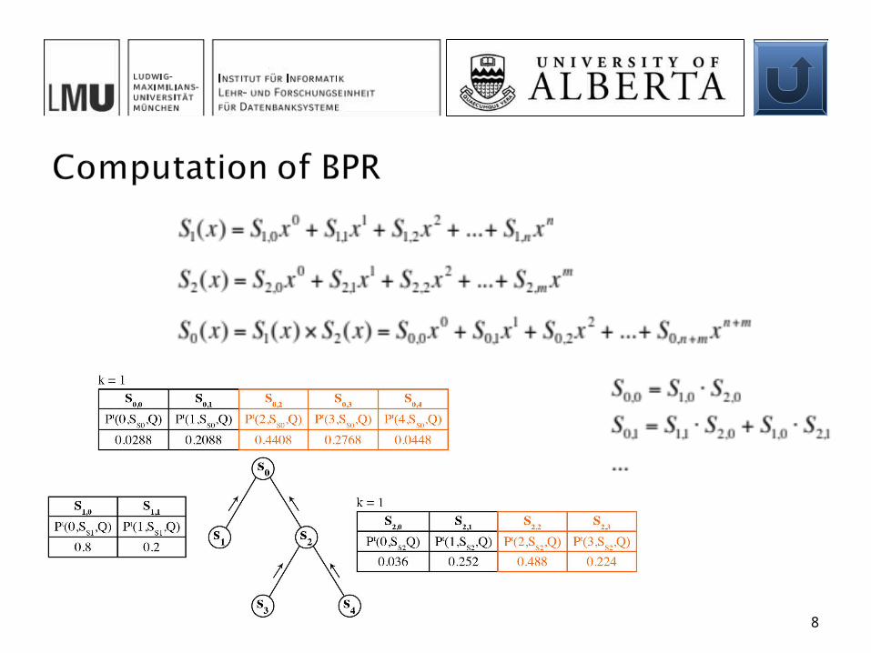
We can solve the problem of computing the probabilistic counts efficiently by using the Poisson Binomial Recurrence

and

Exactly k: , at most k: and at

least k:

k

j

SjPSkP0

),(),(

1

0

),(1),(k

j

SjPSkP

),( SkP

7

8

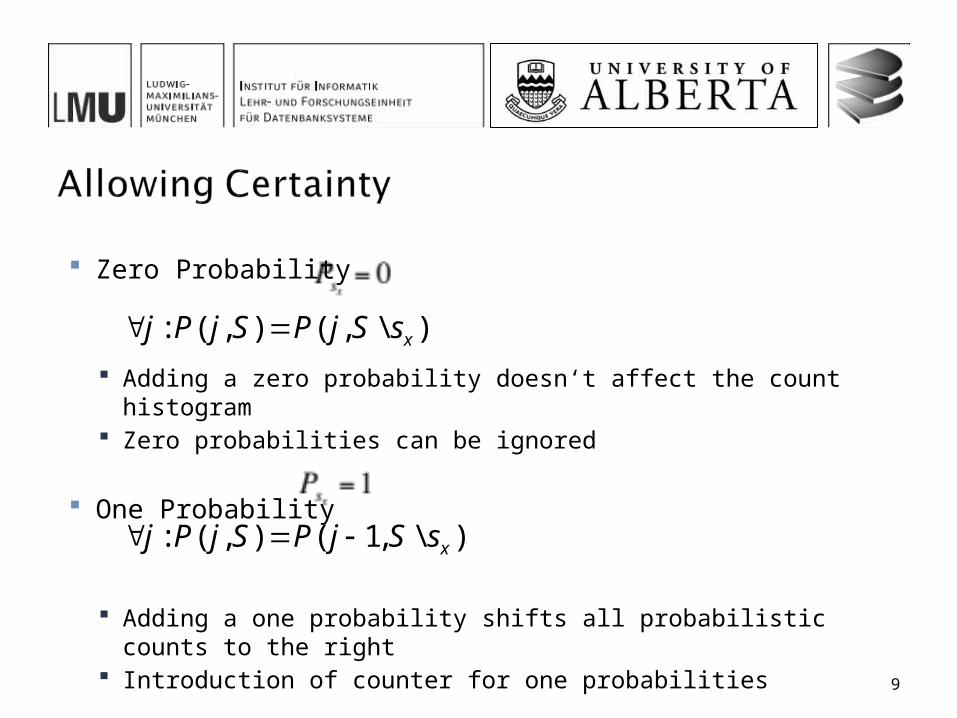
Zero Probability

Adding a zero probability doesn‘t affect the count histogram Zero probabilities can be ignored

One Probability

Adding a one probability shifts all probabilistic counts to the right

Introduction of counter for one probabilities

)\,(),(: xsSjPSjPj

)\,1(),(: xsSjPSjPj

9

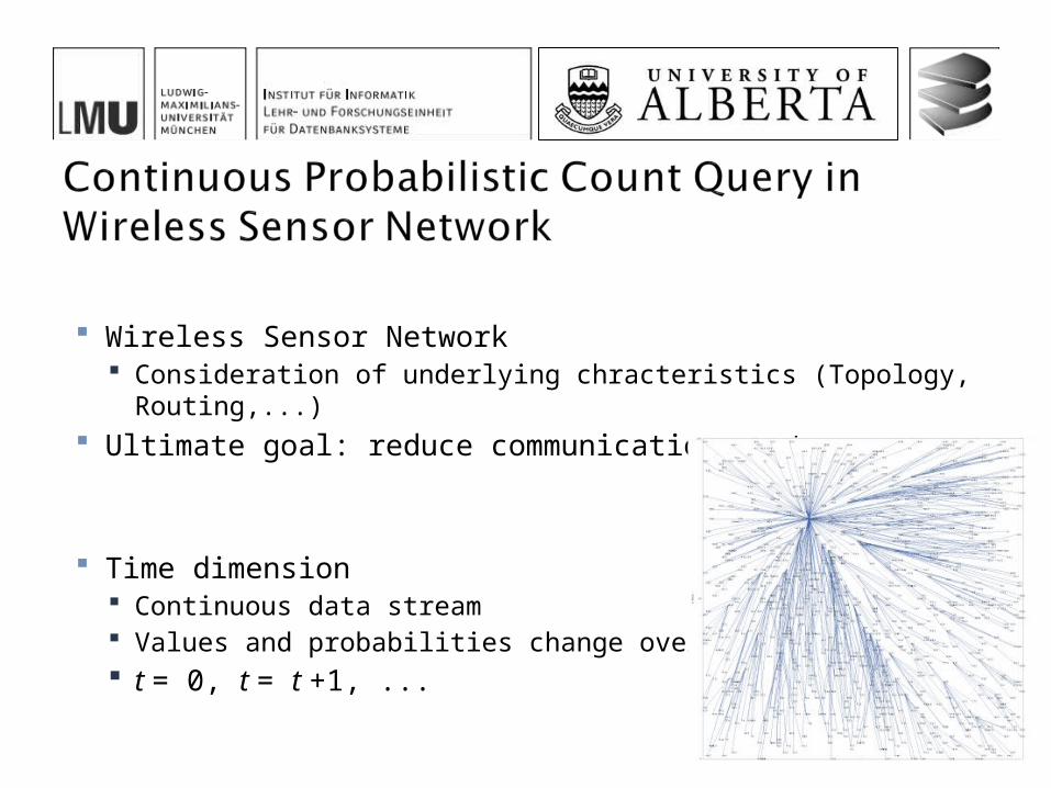
Wireless Sensor Network Consideration of underlying chracteristics (Topology, Routing,...)

Ultimate goal: reduce communication cost

Time dimension Continuous data stream Values and probabilities change over time t = 0, t = t +1, ...

10

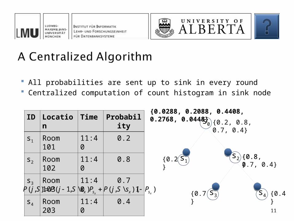
All probabilities are sent up to sink in every round Centralized computation of count histogram in sink node

s2

s3 s4

s0

s1

{0.4}{0.7}

{0.8}{0.2} {0.8, 0.7, 0.4}

{0.2, 0.8, 0.7, 0.4}ID Location Time Probability

s1 Room 101 11:40 0.2

s2 Room 102 11:40 0.8

s3 Room 103 11:40 0.7

s4 Room 203 11:40 0.4

)1)(\,()\,1(),(xx sxsx PsSjPPsSjPSjP

{0.0288, 0.2088, 0.4408, 0.2768, 0.0448}

11

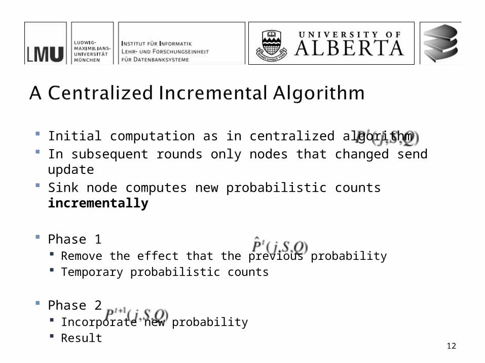
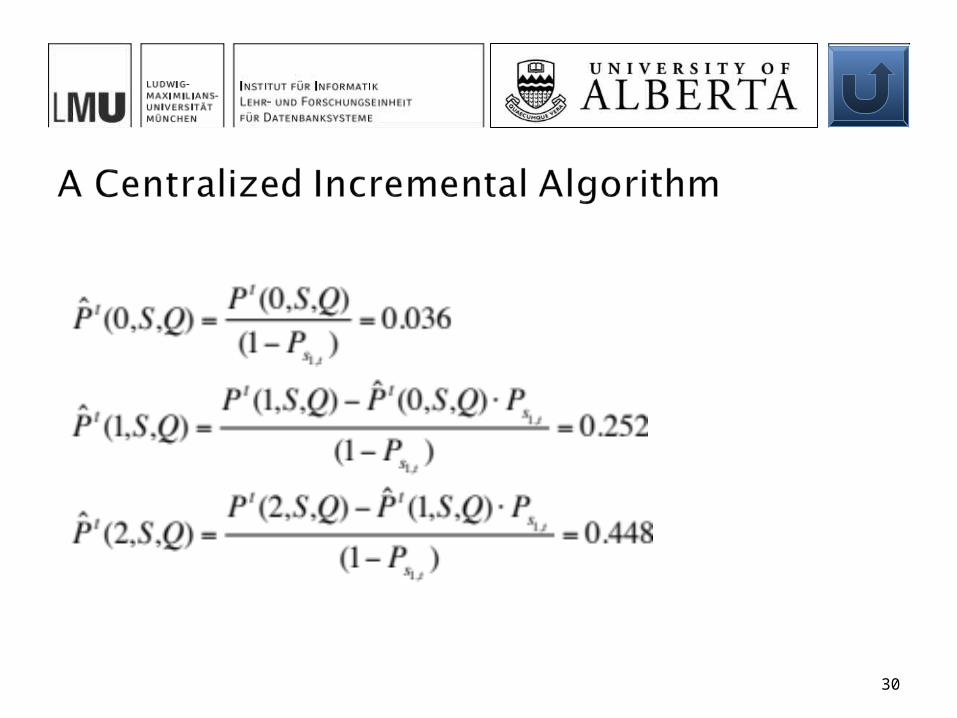
Initial computation as in centralized algorithm In subsequent rounds only nodes that changed send update Sink node computes new probabilistic counts incrementally

Phase 1 Remove the effect that the previous probability Temporary probabilistic counts

Phase 2 Incorporate new probability Result

12

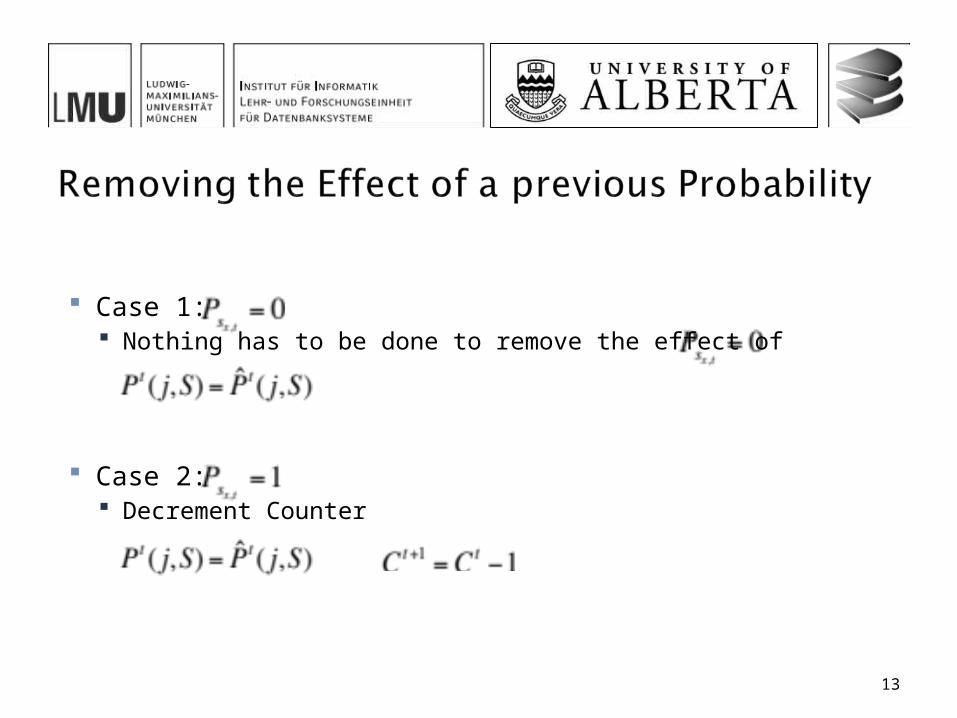
Case 1: Nothing has to be done to remove the effect of

Case 2: Decrement Counter

13

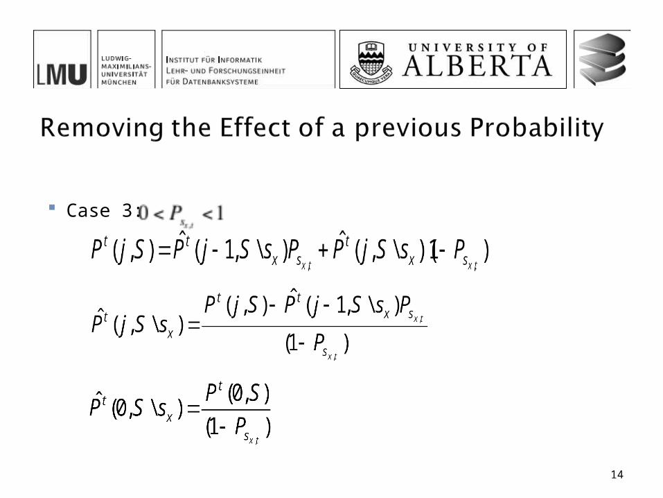
Case 3:

14

Case 1:Nothing has to be done to incorporate the effect of

Case 2:Increment Counter

Case 3:

),(),(ˆ SjPSjP tt

),(),(ˆ 1 SjPSjP tt

)1)(\,(ˆ)\,1(ˆ),(1,1,

1

txtx sxsxt PsSjPPsSjPSjP

15

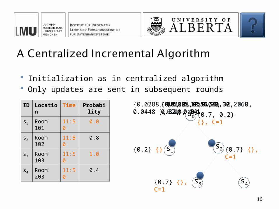
Initialization as in centralized algorithm Only updates are sent in subsequent rounds

s2

s3 s4

s0

s1

{0.7} {}, C=1

{0.2} {} {0.7} {}, C=1

{0.7, 0.2} {}, C=1

ID Location Time Probability

s1 Room 101 11:40 0.2

s2 Room 102 11:40 0.8

s3 Room 103 11:40 0.7

s4 Room 203 11:40 0.4

ID Location Time Probability

s1 Room 101 11:50 0.0

s2 Room 102 11:50 0.8

s3 Room 103 11:50 1.0

s4 Room 203 11:50 0.4

{0.12, 0.56, 0.32, 0.0, 0.0}, C=1{0.0288, 0.2088, 0.4408, 0.2768, 0.0448 }, C=0

16

{0.0, 0.12,0.56, 0.32, 0.0}

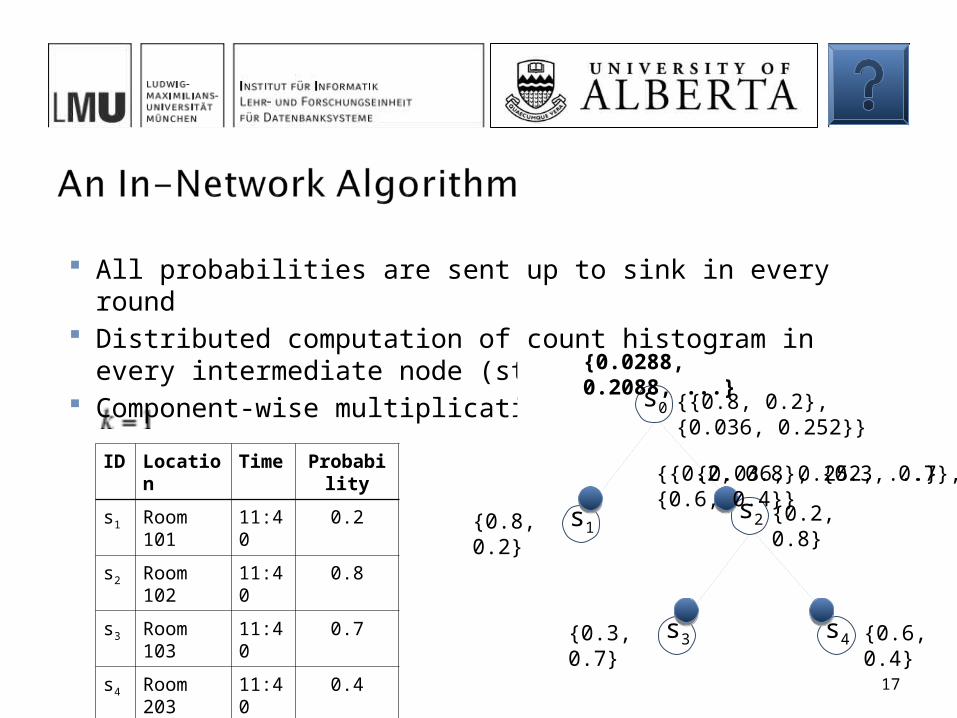
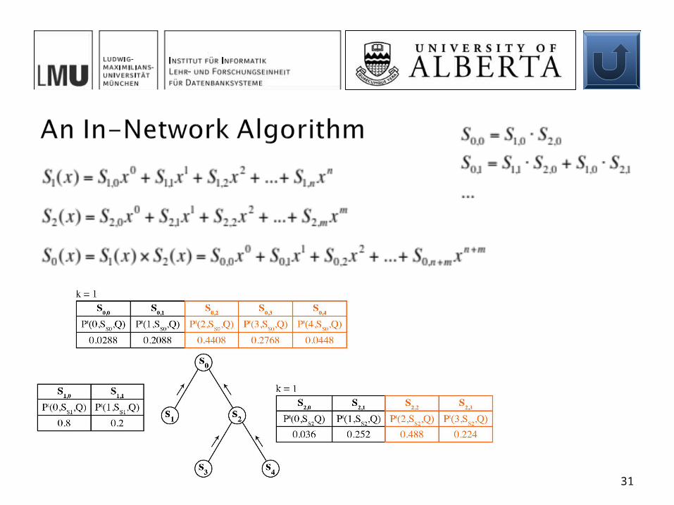
All probabilities are sent up to sink in every round Distributed computation of count histogram in every

intermediate node (stopping at k) Component-wise multiplication

s2

s3 s4

s0

s1

{0.6, 0.4}{0.3, 0.7}

{0.2, 0.8}{0.8, 0.2}

{{0.2, 0.8}, {0.3, 0.7}, {0.6, 0.4}}

{{0.8, 0.2}, {0.036, 0.252}}

ID Location Time Probability

s1 Room 101 11:40 0.2

s2 Room 102 11:40 0.8

s3 Room 103 11:40 0.7

s4 Room 203 11:40 0.4

{0.036, 0.252, ...}

{0.0288, 0.2088, ...}

17

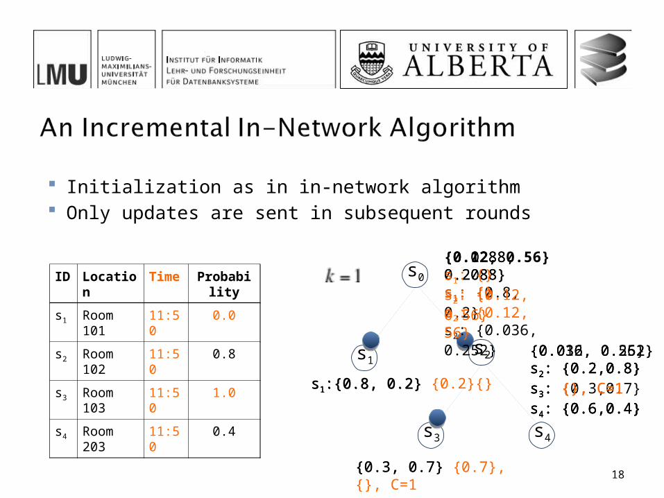
Initialization as in in-network algorithm Only updates are sent in subsequent rounds

{0.036, 0.252}s2: {0.2,0.8}s3: {0.3,0.7}s4: {0.6,0.4}

s2

s3 s4

s0

s1

{0.3, 0.7}

s1:{0.8, 0.2}

{0.012, 0.56}s2: {0.2,0.8}s3: {}, C=1s4: {0.6,0.4}

{0.0288, 0.2088}s1: {0.8, 0.2}s2: {0.036, 0.252}

{0.0288, 0.2088}s1: {}s2: {0.12, 56}

{0.12, 0.56}s1: {}s2: {0.12, 0.56}

{0.036, 0.252}s2: {0.2,0.8}s3: {}, C=1s4: {0.6,0.4}

18

ID Location Time Probability

s1 Room 101 11:40 0.2

s2 Room 102 11:40 0.8

s3 Room 103 11:40 0.7

s4 Room 203 11:40 0.4

ID Location Time Probability

s1 Room 101 11:50 0.0

s2 Room 102 11:50 0.8

s3 Room 103 11:50 1.0

s4 Room 203 11:50 0.4

s1:{0.8, 0.2} {0.2}{}

{0.3, 0.7} {0.7}, {}, C=1

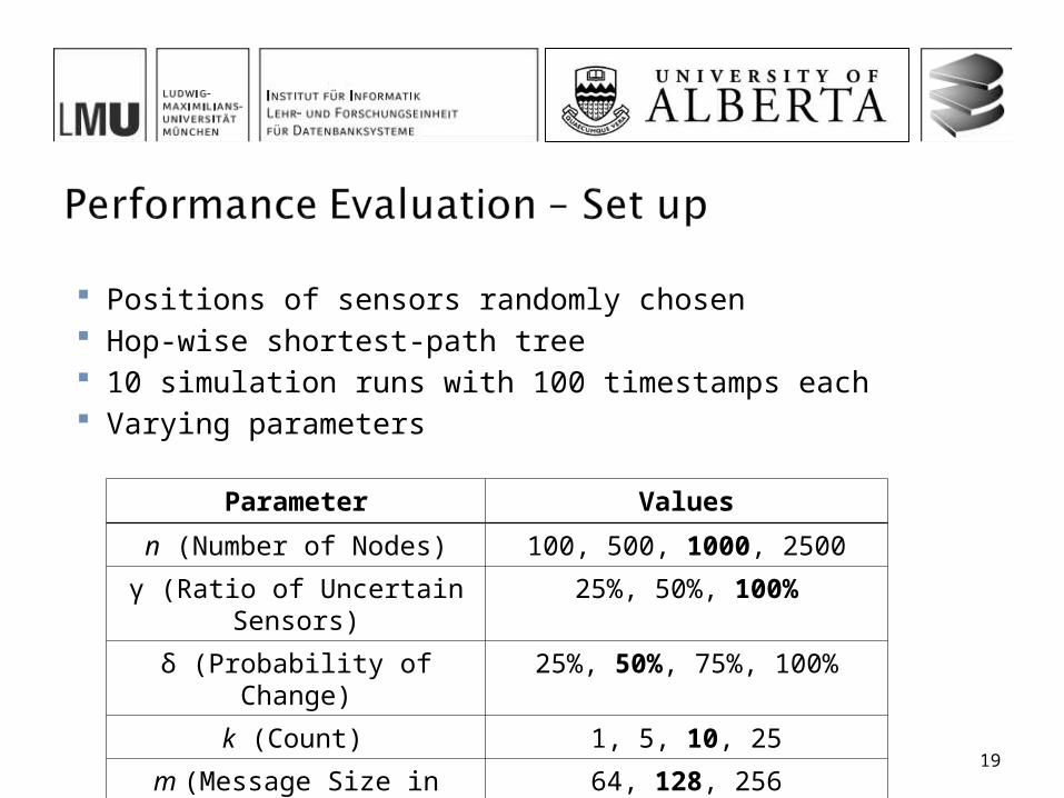
Positions of sensors randomly chosen Hop-wise shortest-path tree 10 simulation runs with 100 timestamps each Varying parameters

Parameter Values

n (Number of Nodes) 100, 500, 1000, 2500

γ (Ratio of Uncertain Sensors) 25%, 50%, 100%

δ (Probability of Change) 25%, 50%, 75%, 100%

k (Count) 1, 5, 10, 25

m (Message Size in bytes) 64, 128, 256

19

20

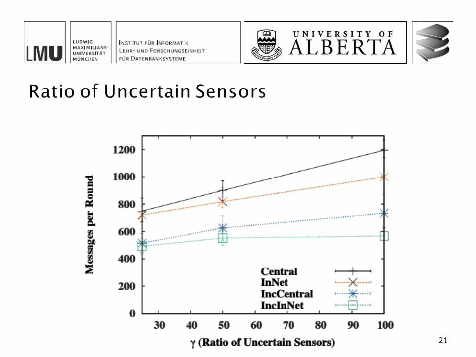
21

22

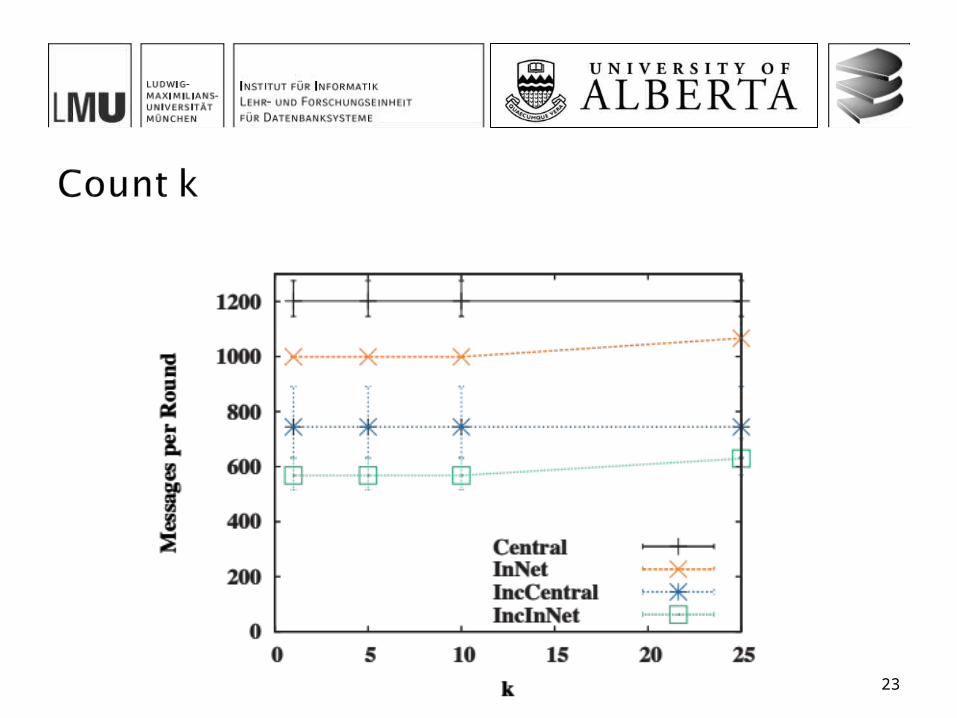
23

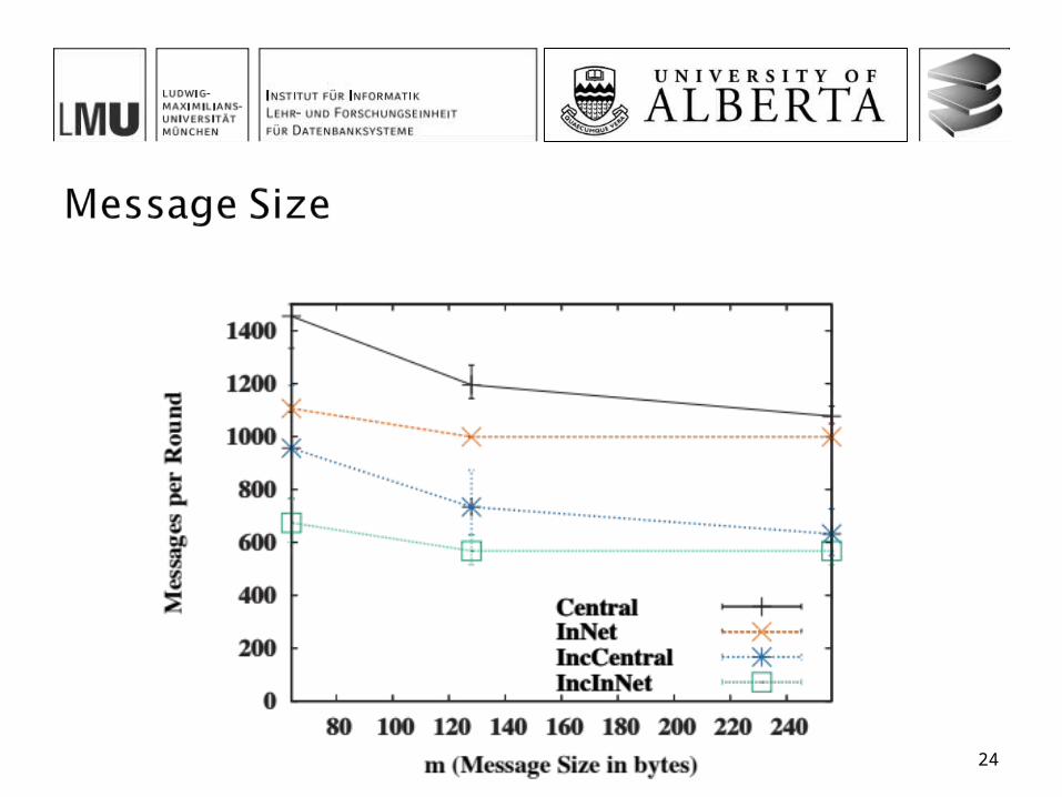
24

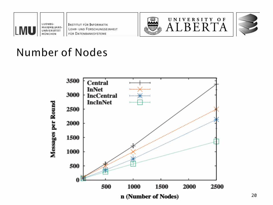
The incremental in-network algorithm offers the best overall performance among all four investigated approaches In particular when the message size is small, there is a small

probability of updates, large networks and high uncertainty and small values of k

Future work: Other types of aggregate queries, e.g., count Explore correlations between sensor readings Explore different network topologies

25

Thanks …

26

...

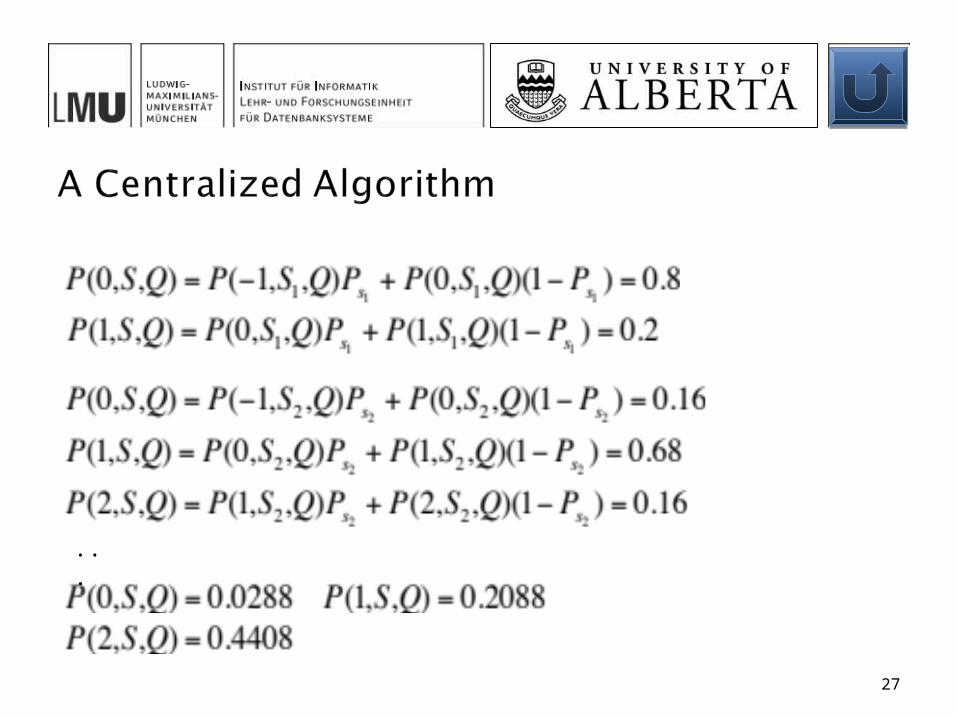
27

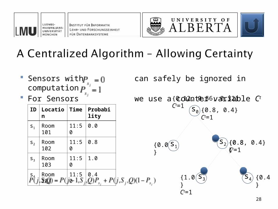
Sensors with can safely be ignored in computation For Sensors we use a counter variable Ct

s2

s3 s4

s0

s1

{0.4}{1.0}Ct=1

{0.8}{0.0} {0.8, 0.4} Ct=1

{0.8, 0.4} Ct=1ID Location Time Probability

s1 Room 101 11:50 0.0

s2 Room 102 11:50 0.8

s3 Room 103 11:50 1.0

s4 Room 203 11:50 0.4

{0.12, 0.56, 0.32} Ct=1

28

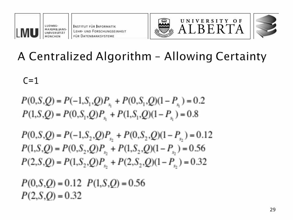
C=1

29

30

31