Embed Size (px)
Citation preview
Continuous-time Principal-Agent Problems:
Necessary and Sufficient Conditions for
Optimality∗
Jaksa Cvitanic †
Xuhu Wan‡
Jianfeng Zhang §
This draft: August 03, 2004.
Key Words and Phrases: Principal-Agent problems, executive compensation, optimal
contracts and incentives, stochastic maximum principle, Forward-Backward SDEs.
AMS (2000) Subject Classifications: 91B28, 93E20; JEL Classification: M52
∗Research supported in part by NSF grants DMS 00-99549 and DMS 04-03575.†Departments of Mathematics and Economics, USC, 3620 S Vermont Ave, MC 2532, Los Angeles, CA
90089-1113. Ph: (213) 740-3794. Fax: (213) 740-2424. E-mail: [email protected].‡Department of Mathematics , USC, 3620 S Vermont Ave, MC 2532, Los Angeles, CA 90089-1113. Ph:
(213) 447-5148. E-mail: [email protected].§Department of Mathematics, USC, 3620 S Vermont Ave, MC 2532, Los Angeles, CA 90089-1113. Ph:
(213) 740-9805. E-mail: [email protected].

Abstract
In this paper we present a unified approach to solving principal-agent problems inmodels driven by Brownian Motion. We apply the stochastic maximum principle togive necessary and sufficient conditions for optimal contracts, for both the symmetricinformation case and the hidden information case. We also make a distinction betweenthe case of the utility from the payoff being separable or not separable from the penaltyon the agent’s effort. Our methodology covers a number of frameworks consideredin the existing literature. The main finance application of this theory is optimalcompensation of company executives.

1 Introduction
In recent years there has been a significant revival of interest in the so-called principal-
agent problems from economics and finance. In particular, a number of recent papers study
these problems in continuous time. Main applications include optimal reward of portfolio
managers and optimal compensation of company executives. A nice survey is provided by
Sung (2001).
Principal-agent problems involve an interaction between two parties to a contract: an
agent and a principal. Through the contract, the principal tries to induce the agent to act
in line with the principal’s interests. In this paper, we consider principal-agent problems
in continuous time, in which both the volatility (the diffusion coefficient) and the drift
of the underlying process can be controlled by the agent. The pioneering paper in the
continuous-time framework is Holmstrom and Milgrom (1987), which showed that if both
the principal and the agent have exponential utilities, then the optimal contract is linear.
In their framework, the principal cannot directly observe the actions of the agent (called
“hidden information” case), who controls the drift only. Subsequently, Schattler and Sung
(1993) generalized those results using a dynamic programming and martingales approach
of Stochastic Control Theory, and Sung (1995) showed that the linearity of the optimal
contract still holds even if the agent can control the volatility, too. More complex models
are considered in Detemple, Govindaraj and Loewenstein (2001). In Ou-Yang (2003), the
agent controls the volatility only, and the issue of hidden information does not come up
here, because in continuous time the volatility can be deduced from observing the controlled
process. That article uses HJB equations as the technical tool. In Cadenillas, Cvitanic and
Zapatero (2003) the results of Ou-Yang (2003) have been generalized to a setting where
the drift is also controlled by the agent, and the principal observes it. They use duality-
martingale methods, familiar from the portfolio optimization theory. The paper closest to
ours is Williams (2004). That paper uses the stochastic maximum principle to characterize
the optimal contract in the principal-agent problems with hidden information, in the case of
the penalty on the agent’s effort being separate (outside) of his utility, and without volatility
control.
In the first part of the paper, we use the same setting, but in the case of full information,
and also with possibly non-separable utility. This provides a general theory for the special
problems considered in Ou-Yang (2003) and Cadenillas et al. (2003). In the second part
we study the hidden information case with separable utility, and, unlike Williams (2004),
we prove our results from the scratch, thus getting them under weaker conditions, while
Williams (2004) mostly refers to existing literature for the proofs. In fact, the stochastic
control literature that uses “weak formulation” usually assumes bounded controls, while we
1
allow more general controls. Williams (2004) paper also deals with the so-called hidden
states case and continuously paid reward, which we do not discuss here. With the exception
of the latter, our framework contains all of the above mentioned models.
In most of the cases, we do not discuss the existence of the optimal control. Instead, the
stochastic maximum principle enables us to characterize the optimal contract via a solution
to Forward-Backward Stochastic Differential Equations (FBSDEs), possibly fully coupled.
However, we do not know under which general conditions these equations have a solution.
The stochastic maximum principle is covered in the book Yong and Zhou (1999), while
FBSDEs are studied in the monograph Ma and Yong (1999).
The paper is organized as follows: In Section 2 we analyze the principal-agent problem
with full information. We find the so-called first best solution, which is the one that corre-
sponds to the best controls from the principal’s point of view. We show that those controls
are implementable, that is, there is a contract which induces the agent to implement the
first best controls. In Section 3, we consider the problem with hidden information. Using a
weak formulation for stochastic control problems, we first find the necessary conditions for
implementable contracts by solving the agent’s problem, and then we discuss the charac-
terization of the optimal contract to be offered by the principal. We conclude in Section 4,
mentioning possible further research topics.
2 Full information; the first best controls
In this section we assume that the principal can observe the actions of the agent. In this case
it turns out that the principal can induce the agent to use the controls which are optimal
for the principal. The contract that achieves this is called the first best contract.
2.1 The model
Let Wtt≥0 be a d-dimensional Brownian Motion on a probability space (Ω,F , P ) and
denote by F := Ftt≤T its augmented filtration on the interval [0, T ]. The controlled state
process is denoted X = Xu,v and its dynamics are given by
dXt = f(t,Xt, ut, vt)dt+ vtdWt (2.1)
where (X, u, v) take values in IR× IRm× IRd, and f is a function taking values in IR, possibly
random and such that, as a process, it is F-adapted. The notation xy for two vectors
x, y ∈ IRd indicates the inner product.
In the principal-agent problems, the principal gives the agent compensation CT which is
payable at time T and is a FT -measurable random variable. The agent chooses the controls
2
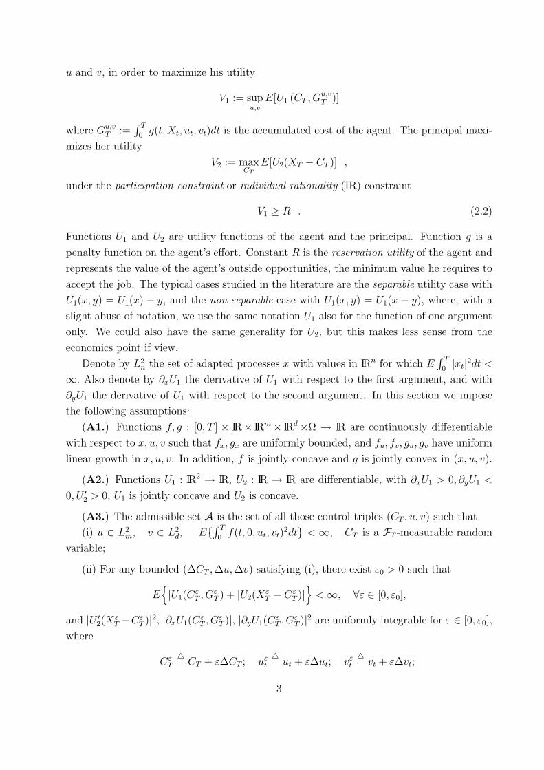
u and v, in order to maximize his utility
V1 := supu,v
E[U1 (CT , Gu,vT )]
where Gu,vT :=
∫ T0g(t,Xt, ut, vt)dt is the accumulated cost of the agent. The principal maxi-
mizes her utility
V2 := maxCT
E[U2(XT − CT )] ,
under the participation constraint or individual rationality (IR) constraint
V1 ≥ R . (2.2)
Functions U1 and U2 are utility functions of the agent and the principal. Function g is a
penalty function on the agent’s effort. Constant R is the reservation utility of the agent and
represents the value of the agent’s outside opportunities, the minimum value he requires to
accept the job. The typical cases studied in the literature are the separable utility case with
U1(x, y) = U1(x) − y, and the non-separable case with U1(x, y) = U1(x − y), where, with a
slight abuse of notation, we use the same notation U1 also for the function of one argument
only. We could also have the same generality for U2, but this makes less sense from the
economics point if view.
Denote by L2n the set of adapted processes x with values in IRn for which E
∫ T0|xt|2dt <
∞. Also denote by ∂xU1 the derivative of U1 with respect to the first argument, and with
∂yU1 the derivative of U1 with respect to the second argument. In this section we impose
the following assumptions:
(A1.) Functions f, g : [0, T ] × IR× IRm× IRd×Ω → IR are continuously differentiable
with respect to x, u, v such that fx, gx are uniformly bounded, and fu, fv, gu, gv have uniform
linear growth in x, u, v. In addition, f is jointly concave and g is jointly convex in (x, u, v).
(A2.) Functions U1 : IR2 → IR, U2 : IR → IR are differentiable, with ∂xU1 > 0, ∂yU1 <
0, U ′2 > 0, U1 is jointly concave and U2 is concave.
(A3.) The admissible set A is the set of all those control triples (CT , u, v) such that
(i) u ∈ L2m, v ∈ L2
d, E∫ T0f(t, 0, ut, vt)
2dt < ∞, CT is a FT -measurable random
variable;
(ii) For any bounded (∆CT ,∆u,∆v) satisfying (i), there exist ε0 > 0 such that
E|U1(Cε
T , GεT ) + |U2(Xε
T − CεT )|<∞, ∀ε ∈ [0, ε0],
and |U ′2(XεT −Cε
T )|2, |∂xU1(CεT , G
εT )|, |∂yU1(Cε
T , GεT )|2 are uniformly integrable for ε ∈ [0, ε0],
where
CεT
4= CT + ε∆CT ; uεt
4= ut + ε∆ut; vεt
4= vt + ε∆vt;
3
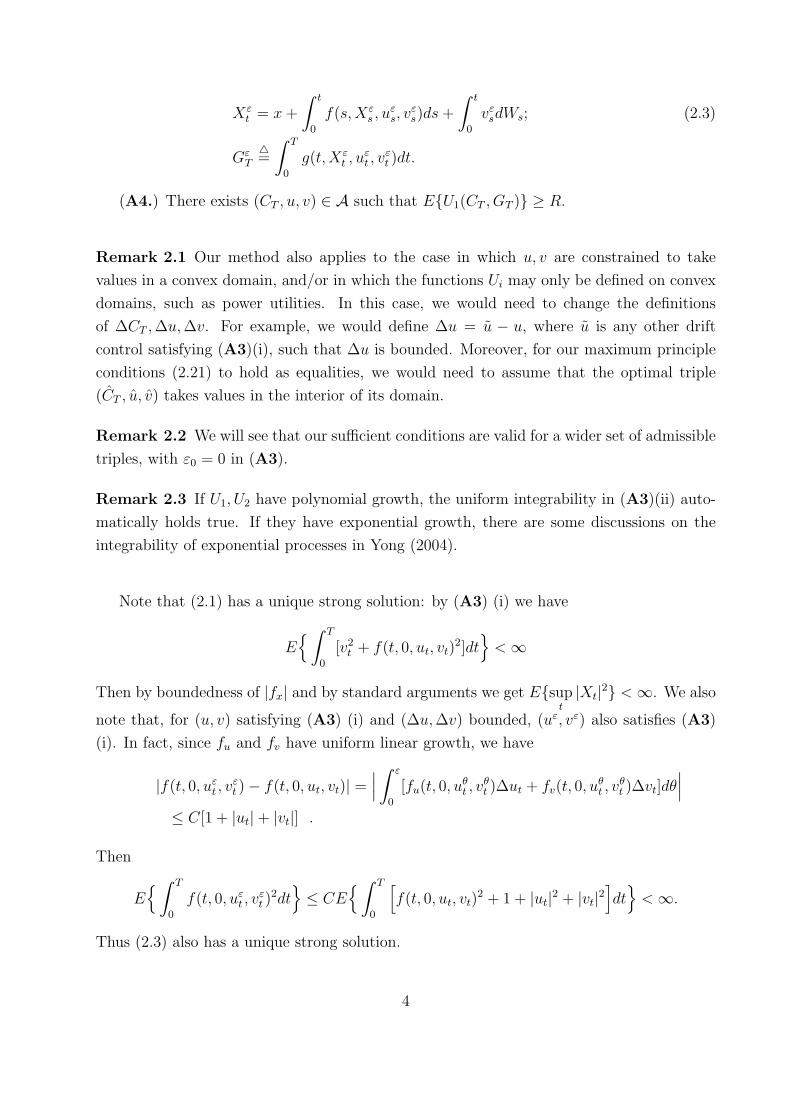
Xεt = x+
∫ t
0
f(s,Xεs , u
εs, v
εs)ds+
∫ t
0
vεsdWs; (2.3)
GεT
4=
∫ T
0
g(t,Xεt , u
εt , v
εt )dt.
(A4.) There exists (CT , u, v) ∈ A such that EU1(CT , GT ) ≥ R.
Remark 2.1 Our method also applies to the case in which u, v are constrained to take
values in a convex domain, and/or in which the functions Ui may only be defined on convex
domains, such as power utilities. In this case, we would need to change the definitions
of ∆CT ,∆u,∆v. For example, we would define ∆u = u − u, where u is any other drift
control satisfying (A3)(i), such that ∆u is bounded. Moreover, for our maximum principle
conditions (2.21) to hold as equalities, we would need to assume that the optimal triple
(CT , u, v) takes values in the interior of its domain.
Remark 2.2 We will see that our sufficient conditions are valid for a wider set of admissible
triples, with ε0 = 0 in (A3).
Remark 2.3 If U1, U2 have polynomial growth, the uniform integrability in (A3)(ii) auto-
matically holds true. If they have exponential growth, there are some discussions on the
integrability of exponential processes in Yong (2004).
Note that (2.1) has a unique strong solution: by (A3) (i) we have
E∫ T
0
[v2t + f(t, 0, ut, vt)
2]dt<∞
Then by boundedness of |fx| and by standard arguments we get Esupt|Xt|2 <∞. We also
note that, for (u, v) satisfying (A3) (i) and (∆u,∆v) bounded, (uε, vε) also satisfies (A3)
(i). In fact, since fu and fv have uniform linear growth, we have
|f(t, 0, uεt , vεt )− f(t, 0, ut, vt)| =
∣∣∣∫ ε
0
[fu(t, 0, uθt , v
θt )∆ut + fv(t, 0, u
θt , v
θt )∆vt]dθ
∣∣∣≤ C[1 + |ut|+ |vt|] .
Then
E∫ T
0
f(t, 0, uεt , vεt )
2dt≤ CE
∫ T
0
[f(t, 0, ut, vt)
2 + 1 + |ut|2 + |vt|2]dt<∞.
Thus (2.3) also has a unique strong solution.
4

We first consider the so-called first best contract: in this setting it is actually the principal
who chooses the controls u and v, and provides the agent with compensation CT so that the
IR constraint is satisfied. In other words, the principal’s value function is
V2 = supCT ,u,v
E[U2(XT − CT )] (2.4)
where (CT , u, v) ∈ A is chosen so that
E[U1 (CT , Gu,vT )] ≥ R .
In fact, later on we will also check that (under some conditions), if (CT , u, v) is the optimal
solution to this problem, then there is a contract C∗ such that (u, v) is optimal for the
agent’s problem V1 = V1(C∗), and that C∗ = C when (u, v) is used. We say that the
contract (C, u, v) is implementable.
We define the Lagrangian as follows, for a given constant λ > 0:
J(CT , u, v;λ) = E[U2(Xu,vT − CT ) + λ(U1(CT , G
u,vT )−R)] (2.5)
Because of our assumptions, by the standard optimization theory (see Luenberger 1969), we
have
V2 = supCT ,u,v
J(CT , u, v; λ) (2.6)
for some λ > 0. Moreover, if the maximum is attained in (2.4) by (CT , u, v), then it is
attained by the same triple in the right-hand side of (2.6), and we have
E[U1(CT , Gu,vT )] = R .
Conversely, if there exists λ > 0 and (CT , u, v) such that the maximum is attained in the
right-hand side of (2.6) and such that E[U1(CT , Gu,vT )] = R, then (CT , u, v) is also optimal
for the problem V2 of (2.4).
2.2 Necessary conditions for optimality
We could use standard approaches to deriving necessary conditions for optimality, as pre-
sented, for example, in the book Yong and Zhou (1999). However, since our optimization
problem has a somewhat non-standard form, and we will need similar arguments in Section
3, we present here a proof starting from the scratch.
Fix λ and suppose that (CT , u, v) ∈ A and (∆CT ,∆u,∆v) is uniformly bounded. Let
ε0 > 0 be the constant determined in (A3) (iii). For ε ∈ (0, ε0), recall (2.3) and denote
Jε4= J(Cε
T , uε, vε); J
4= J(CT , u, v);
∇Xεt
4=Xεt −Xt
ε; ∇Gε
T
4=GεT −GT
ε; ∇Jε 4= Jε − J
ε. (2.7)
5
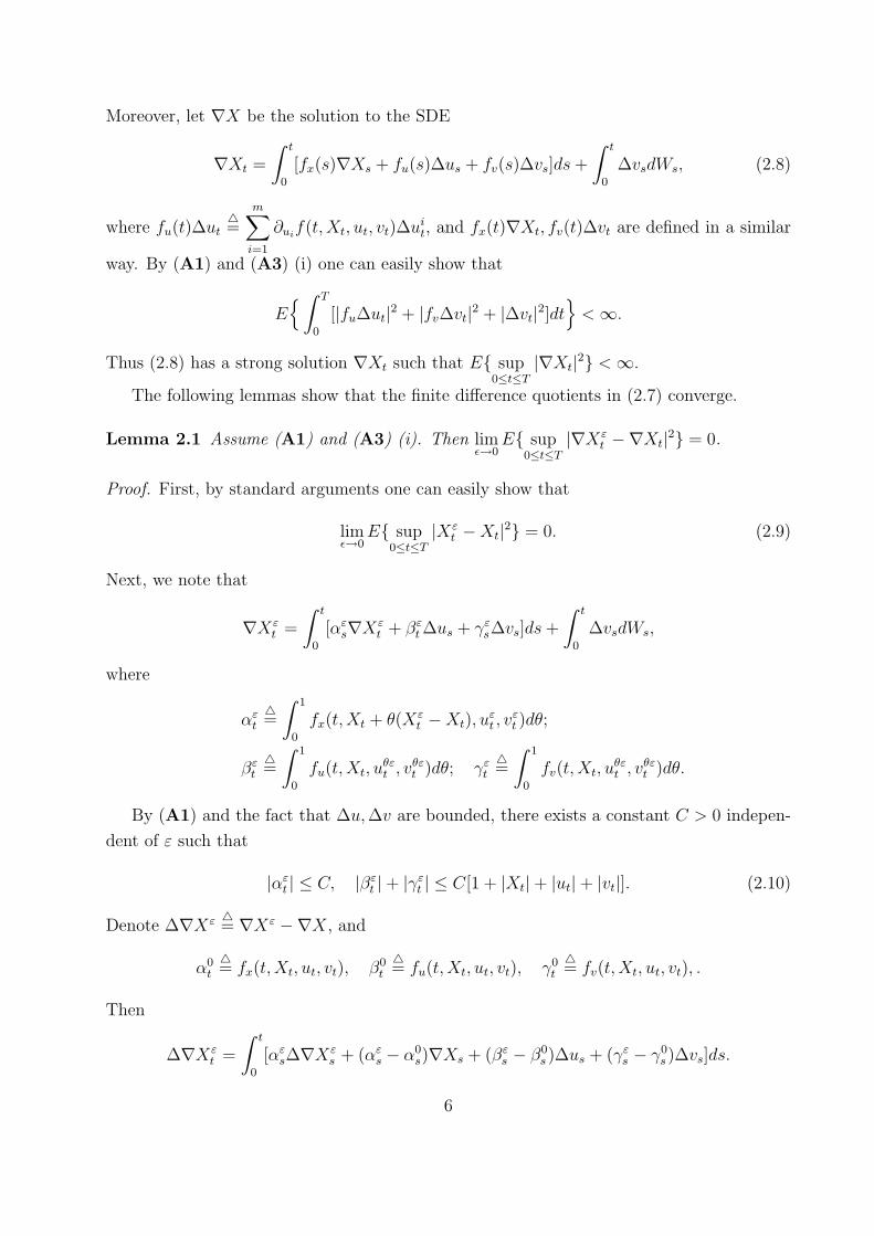
Moreover, let ∇X be the solution to the SDE
∇Xt =
∫ t
0
[fx(s)∇Xs + fu(s)∆us + fv(s)∆vs]ds+
∫ t
0
∆vsdWs, (2.8)
where fu(t)∆ut4=
m∑i=1
∂uif(t,Xt, ut, vt)∆uit, and fx(t)∇Xt, fv(t)∆vt are defined in a similar
way. By (A1) and (A3) (i) one can easily show that
E∫ T
0
[|fu∆ut|2 + |fv∆vt|2 + |∆vt|2]dt<∞.
Thus (2.8) has a strong solution ∇Xt such that E sup0≤t≤T
|∇Xt|2 <∞.
The following lemmas show that the finite difference quotients in (2.7) converge.
Lemma 2.1 Assume (A1) and (A3) (i). Then limε→0
E sup0≤t≤T
|∇Xεt −∇Xt|2 = 0.
Proof. First, by standard arguments one can easily show that
limε→0
E sup0≤t≤T
|Xεt −Xt|2 = 0. (2.9)
Next, we note that
∇Xεt =
∫ t
0
[αεs∇Xεt + βεt∆us + γεs∆vs]ds+
∫ t
0
∆vsdWs,
where
αεt4=
∫ 1
0
fx(t,Xt + θ(Xεt −Xt), u
εt , v
εt )dθ;
βεt4=
∫ 1
0
fu(t,Xt, uθεt , v
θεt )dθ; γεt
4=
∫ 1
0
fv(t,Xt, uθεt , v
θεt )dθ.
By (A1) and the fact that ∆u,∆v are bounded, there exists a constant C > 0 indepen-
dent of ε such that
|αεt | ≤ C, |βεt |+ |γεt | ≤ C[1 + |Xt|+ |ut|+ |vt|]. (2.10)
Denote ∆∇Xε 4= ∇Xε −∇X, and
α0t
4= fx(t,Xt, ut, vt), β0
t
4= fu(t,Xt, ut, vt), γ0
t
4= fv(t,Xt, ut, vt), .
Then
∆∇Xεt =
∫ t
0
[αεs∆∇Xεs + (αεs − α0
s)∇Xs + (βεs − β0s )∆us + (γεs − γ0
s )∆vs]ds.
6
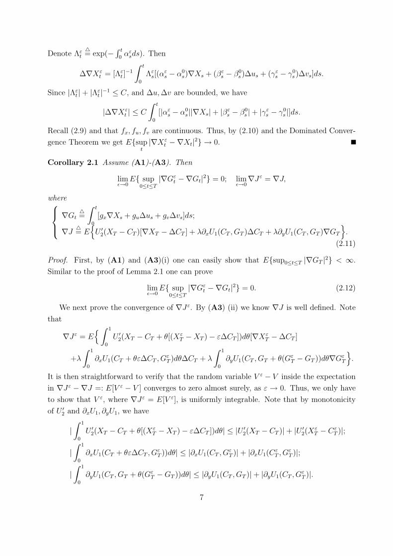
Denote Λεt
4= exp(− ∫ t
0αεsds). Then
∆∇Xεt = [Λε
t ]−1
∫ t
0
Λεs[(α
εs − α0
s)∇Xs + (βεs − β0s )∆us + (γεs − γ0
s )∆vs]ds.
Since |Λεt |+ |Λε
t |−1 ≤ C, and ∆u,∆v are bounded, we have
|∆∇Xεt | ≤ C
∫ t
0
[|αεs − α0s||∇Xs|+ |βεs − β0
s |+ |γεs − γ0s |]ds.
Recall (2.9) and that fx, fu, fv are continuous. Thus, by (2.10) and the Dominated Conver-
gence Theorem we get Esupt|∇Xε
t −∇Xt|2 → 0.
Corollary 2.1 Assume (A1)-(A3). Then
limε→0
E sup0≤t≤T
|∇Gεt −∇Gt|2 = 0; lim
ε→0∇Jε = ∇J,
where∇Gt
4=
∫ t
0
[gx∇Xs + gu∆us + gv∆vs]ds;
∇J 4= EU ′2(XT − CT )[∇XT −∆CT ] + λ∂xU1(CT , GT )∆CT + λ∂yU1(CT , GT )∇GT
.
(2.11)
Proof. First, by (A1) and (A3)(i) one can easily show that Esup0≤t≤T |∇GT |2 < ∞.
Similar to the proof of Lemma 2.1 one can prove
limε→0
E sup0≤t≤T
|∇Gεt −∇Gt|2 = 0. (2.12)
We next prove the convergence of ∇Jε. By (A3) (ii) we know ∇J is well defined. Note
that
∇Jε = E∫ 1
0
U ′2(XT − CT + θ[(XεT −XT )− ε∆CT ])dθ[∇Xε
T −∆CT ]
+λ
∫ 1
0
∂xU1(CT + θε∆CT , GεT )dθ∆CT + λ
∫ 1
0
∂yU1(CT , GT + θ(GεT −GT ))dθ∇Gε
T
.
It is then straightforward to verify that the random variable V ε − V inside the expectation
in ∇Jε −∇J =: E[V ε − V ] converges to zero almost surely, as ε → 0. Thus, we only have
to show that V ε, where ∇Jε = E[V ε], is uniformly integrable. Note that by monotonicity
of U ′2 and ∂xU1, ∂yU1, we have
|∫ 1
0
U ′2(XT − CT + θ[(XεT −XT )− ε∆CT ])dθ| ≤ |U ′2(XT − CT )|+ |U ′2(Xε
T − CεT )|;
|∫ 1
0
∂xU1(CT + θε∆CT , GεT ))dθ| ≤ |∂xU1(CT , G
εT )|+ |∂xU1(Cε
T , GεT )|;
|∫ 1
0
∂yU1(CT , GT + θ(GεT −GT ))dθ| ≤ |∂yU1(CT , GT )|+ |∂yU1(CT , G
εT )|.
7

Using this we get, for a generic constant C,
E[|V e|] ≤ E|U ′2(XT − CT )|+ |U ′2(Xε
T − CεT )||[∇Xε
T −∆CT ]|
+λ(|∂xU1(CT , GεT )|+ |∂xU1(Cε
T , GεT )|)|∆CT |+ λ(|∂yU1(CT , GT )|+ |∂yU1(CT , G
εT )|)|∇Gε
T |
≤ CE|U ′2(XT − CT )|2 + |U ′2(Xε
T − CεT )|2 + |∂xU1(CT , G
εT )|
+|∂xU1(CεT , G
εT )|+ |∂yU1(CT , GT )|2 + |∂yU1(CT , G
εT )|2 + |[∇Xε
T −∆CT ]|2 + |∇GεT |2. (2.13)
Note that (A3) (ii) also holds true for variation (0,∆u,∆v) (maybe with differenent
ε0). Recalling Lemma 2.1 and (2.12), we conclude that V ε are uniformly integrable on
ε ≤ ε0, for a small enough ε0, and applying the Dominated Convergence Theorem we get
limε→0∇Jε = ∇J .
As is usual when finding necessary conditions for stochastic control problems, we now
introduce appropriate adjoint processes as follows:Y 1t = −λ∂yU1(CT , GT )− ∫ T
tZ1sdWs;
Y 2t = U ′2(XT − CT )− ∫ T
t[Y 1s gx(s,Xs, us, vs)− Y 2
s fx(s,Xs, us, vs)]ds−∫ TtZ2sdWs.
(2.14)
Each of these is a Backward Stochastic Differential Equation (BSDE), whose solution is a
pair of adapted processes (Y i, Z i), i = 1, 2. Note that in the case U1(x, y) = U1(x) − y we
have Y 1t ≡ λ, Z1
t ≡ 0. Also note that (A3) (ii) guarantees that the solution (Y 1, Z1) to the
first BSDE exists. Then by the fact that fx, gx are bounded and by (A3) (ii) again, the
solution (Y 2, Z2) to the second BSDE also exists. Moreover, by the BSDE theory, we have
E
sup0≤t≤T
[|Y 1t |2 + |Y 2
t |2] +
∫ T
0
[|Z1t |2 + |Z2
t |2]dt<∞. (2.15)
Theorem 2.1 Assume (A1)-(A3). Then
∇J = E
Γ1T∆CT +
∫ T
0
[Γ2t∆ut + Γ3
t∆vt]dt,
where
Γ1T
4= λ∂xU1(CT , GT )− U ′2(XT − CT );
Γ2t
4= Y 2
t fu(t,Xt, ut, vt)− Y 1t gu(t,Xt, ut, vt);
Γ3t
4= Y 2
t fv(t,Xt, ut, vt)− Y 1t gv(t,Xt, ut, vt) + Z2
t .
(2.16)
Proof. By (2.11) and (2.14), obviously we have
∇J = E
Γ1T∆CT + Y 2
T∇XT − Y 1T∇GT
. (2.17)
Recalling (2.8), (2.11) and (2.14), and applying Ito’s formula we have
d(Y 2t ∇Xt − Y 1
t ∇Gt) = [Γ2t∆ut + Γ3
t∆vt]dt+ Γ4tdWt, (2.18)
8
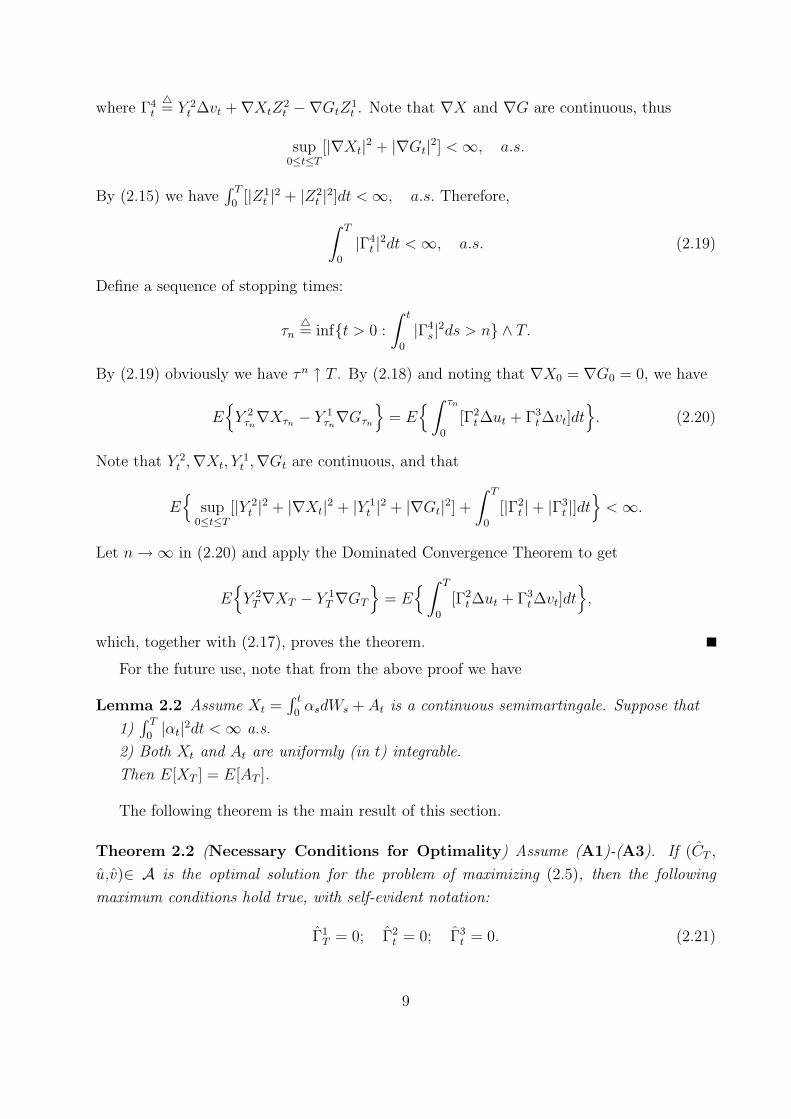
where Γ4t
4= Y 2
t ∆vt +∇XtZ2t −∇GtZ
1t . Note that ∇X and ∇G are continuous, thus
sup0≤t≤T
[|∇Xt|2 + |∇Gt|2] <∞, a.s.
By (2.15) we have∫ T
0[|Z1
t |2 + |Z2t |2]dt <∞, a.s. Therefore,
∫ T
0
|Γ4t |2dt <∞, a.s. (2.19)
Define a sequence of stopping times:
τn4= inft > 0 :
∫ t
0
|Γ4s|2ds > n ∧ T.
By (2.19) obviously we have τn ↑ T . By (2.18) and noting that ∇X0 = ∇G0 = 0, we have
EY 2τn∇Xτn − Y 1
τn∇Gτn
= E
∫ τn
0
[Γ2t∆ut + Γ3
t∆vt]dt. (2.20)
Note that Y 2t ,∇Xt, Y
1t ,∇Gt are continuous, and that
E
sup0≤t≤T
[|Y 2t |2 + |∇Xt|2 + |Y 1
t |2 + |∇Gt|2] +
∫ T
0
[|Γ2t |+ |Γ3
t |]dt<∞.
Let n→∞ in (2.20) and apply the Dominated Convergence Theorem to get
EY 2T∇XT − Y 1
T∇GT
= E
∫ T
0
[Γ2t∆ut + Γ3
t∆vt]dt,
which, together with (2.17), proves the theorem.
For the future use, note that from the above proof we have
Lemma 2.2 Assume Xt =∫ t
0αsdWs + At is a continuous semimartingale. Suppose that
1)∫ T
0|αt|2dt <∞ a.s.
2) Both Xt and At are uniformly (in t) integrable.
Then E[XT ] = E[AT ].
The following theorem is the main result of this section.
Theorem 2.2 (Necessary Conditions for Optimality) Assume (A1)-(A3). If (CT ,
u,v)∈ A is the optimal solution for the problem of maximizing (2.5), then the following
maximum conditions hold true, with self-evident notation:
Γ1T = 0; Γ2
t = 0; Γ3t = 0. (2.21)
9

Remark 2.4 If we define the Hamiltonian H as
H(t,Xt, ut, vt, Yt, Zt) := Y 2t f(t,Xt, ut, vt)− Y 1
t g(t,Xt, ut, vt) + Z2t vt
then the last two maximum conditions become
Hu(t, Xt, ut, vt, Yt, Zt) = 0, Hv(t, Xt, ut, vt, Yt, Zt) = 0.
Proof of Theorem 2.2. Since (CT , u, v) is optimal, for any bounded ∆CT ,∆u,∆v and
any small ε > 0 we have Jε ≤ J where Jε and J are defined in the obvious way. Thus
∇Jε ≤ 0. By Corollary 2.1 we get ∇J ≤ 0. In particular, for
∆CT4= sign(Γ1
T ); ∆ut4= sign(Γ2
t ); ∆vt4= sign(∇Γ3
t ),
we have
0 ≥ ∇J = E|Γ1T |+
∫ T
0
[|Γ2t |+ |Γ3
t |]dt,
which obviously proves the theorem.
We next show that the necessary conditions can be written as a coupled Forward-
Backward SDE. To this end, we note that λ > 0. By (A2) we have
∂
∂c[λ∂xU1(c, g)− U ′2(x− c)] = λ∂xxU1(c, g) + U ′′2 (x− c) ≤ 0.
If we have strict inequality, then there exists a function F1 such that for any x, g, value
c4= F1(x, g) is the solution to the equation
λ∂xU1(c, g)− U ′2(x− c) = 0.
Similarly, for y1, y2 > 0, and any (t, x, u, v), by (A1) we know that[ ∂∂u
(y2fu − y1gu)∂∂v
(y2fu − y1gu)∂∂u
(y2fv − y1gv)∂∂v
(y2fv − y1gv)
]= y2
[fuu fuv
fuv fvv
]− y1
[guu guv
guv gvv
]
is negative definite. If it is strictly negative definite, then there exist functions F2, F3
such that for any y1, y2 > 0 and any (t, x, z2), values u4= F2(t, x, y1, y2, z2) and v
4=
F3(t, x, y1, y2, z2) are the solution to the system of equations
y2fu(t, x, u, v)− y1gu(t, x, u, v) = 0; y2fv(t, x, u, v)− y1gv(t, x, u, v) + z2 = 0.
Theorem 2.3 Assume (A1)-(A3), that there exists functions F1, F2, F3 as above, and that
(fugu)(t, x, u, v) > 0 for any (t, x, u, v). If (CT , u, v) ∈ A is the optimal solution for the
problem of maximizing (2.5), then X, Y 1,Y 2,Z1, and Z2 satisfy the following FBSDE:
Xt = x+
∫ t
0
f(s)ds+
∫ t
0
F3(s, Xs, Y1s , Y
2s , Z
2s )dWs;
Y 1t = −λ∂yU1(F1(XT , GT ), GT )−
∫ T
t
Z1sdWs;
Y 2t = U ′2(XT − F1(XT , GT ))−
∫ T
t
[Y 1s gx(s)− Y 2
s fx(s)]ds−∫ T
t
Z2sdWs,
(2.22)
10

where, for ϕ = f, g, fx, gx,
ϕ(s)4= ϕ(s,Xs, F2(s,Xs, Y
1s , Y
2s , Z
2s ), F3(s,Xs, Y
1s , Y
2s , Z
2s )).
Moreover, the optimal controls are
CT = F1(XT , GT ); ut = F2(s, Xs, Y1s , Y
2s , Z
2s ); vt = F3(s, Xs, Y
1s , Y
2s , Z
2s ).
Proof. By Theorem 2.2 we have (2.21). From Γ1T = 0 we get CT = F1(XT , GT ). Since
λ∂yU1 < 0, we have Y 1t > 0. Moreover, by Γ2
t = 0 and the assumption that fugu > 0 we get
Y 2t > 0. Then we have
ut = F2(s, Xs, Y1s , Y
2s , Z
2s ); vt = F3(s, Xs, Y
1s , Y
2s , Z
2s ).
Now by the definition of the processes on the left-hand sides of (2.22), we see that the
right-hand sides are true.
2.3 Sufficient conditions for optimality
Let us assume that there is a multiple (CT , X, Y1, Y 2, Z1, Z2, u, v) that satisfies the necessary
conditions of Theorem 2.2. We want to check that those are also sufficient conditions, that
is, that (CT , u, v) is optimal. Here, it is essential to have the concavity of f and −g. Let
(CT , u, v) be an arbitrary admissible control triple, with corresponding X,G, and we allow
now ε0 = 0 in the assumption (A3). We have
J(CT , u, v)− J(CT , u, v) = E[U2(XT − CT )− U2(XT − CT )] + λ[U1(CT , GT )− U1(CT , GT )] .
By concavity of Ui, the terminal conditions on Y i, and from Γ1 = 0, or, equivalently,
U ′2 = λ∂xU1, suppressing the arguments of these functions, we get
J(CT , u, v)− J(CT , u, v)
≥ E
[(XT −XT )− (CT − CT )]U ′2 + λ[(CT − CT )∂xU1 + (GT −GT )∂yU1]
= E(XT −XT )U ′2 + λ(GT −GT )∂yU1] = EY 2T (XT −XT )− Y 1
T (GT −GT )= E
∫ T0
[Y 2t (f(t)− f(t)) + Z2
t (vt − vt)− Y 1t (g(t)− g(t))− (Xt −Xt)(Y
2t fx(t)− Y 1
t gx(t))]dt
= E∫ T
0[H(t, Xt, ut, vt, Yt, Zt)−H(t,Xt, ut, vt, Yt, Zt)− (Xt −Xt)Hx(t, Xt, ut, vt, Yt, Zt)]dt
Here, the second to last equality is proved using Ito’s rule and the Dominated Convergence
Theorem, and in a similar way as in the proof of Theorem 2.1. Note that Y 1 is positive, as a
martingale with positive terminal value. Then, from Y 2fu = Y 1gu, we know that Y 2t is also
11

positive. Since f and −g are concave in (Xt, ut, vt), this implies that H(t,Xt, ut, vt, Yt, Zt)
is also concave in (Xt, ut, vt), and we have
(Xt −Xt)Hx(t, Xt, ut, vt, Yt, Zt) ≤ H(t, Xt, ut, vt, Yt, Zt)−H(t,Xt, ut, vt, Yt, Zt)
since, by Remark 2.4, ∂uH = ∂vH = 0. Thus, J(CT , u, v)−J(CT , u, v) ≥ 0. We have proved
the following
Theorem 2.4 Under the assumptions of Theorem 2.2,, if CT , u, v, Xt, Y1t , Y
2t , Z
1t , Z
2t ,
satisfy the necessary conditions of Theorem 2.2, and (CT , u, v) is admissible, possibly with
ε0 = 0, then (CT , u, v) is an optimal triple for the problem of maximizing J(CT , u, v;λ).
Remark 2.5 There remains a question of determining the appropriate Lagrange multiplier
λ, if it exists. We now describe the usual way for identifying it, without giving assumptions
for this method to work. Instead, we refer the reader to Luenberger (1969). First, define
V (λ) = supC,u,v
E[U2(Xu,vT − CT ) + λU1(CT , G
u,vT )] .
Then, the appropriate λ is the one that minimizes V (λ)− λR, if it exists. If, for this λ = λ
there exists an optimal control (C, u, v) for the problem on the right-hand side of (2.6), and
if we have U1(CT , Gu,vT ) = R, then (C, u, v) is also optimal for the problem on the left-hand
side of (2.6).
2.4 Implementing the first best contract
We now consider the situation in which the agent chooses the controls (u, v). We assume that
the function U ′2, is a one-to-one function on its domain, with the inverse function denoted
I2(z) := (U ′2)−1(z) . (2.1)
Note that the boundary condition Y 2T = U ′2(XT − CT ) gives CT = XT − I2(Y 2
T ). In the
problem of executive compensation, this has an interpretation of the executive being payed
by the difference between the stock value and a value I2(Y 2T ) of a benchmark portfolio. We
want to see whether the contract of this form indeed induces the agent to apply the first
best controls (u, v). We have the following
Definition 2.1 We say that an admissible triple (CT , u, v) is implementable if there exists
an admissible contract C∗T such that the pair (u, v) is optimal for the agent’s problem of
maximizing E[U1(C∗T , Gu,vT )], and such that C∗T = CT when (u, v) is used.
12
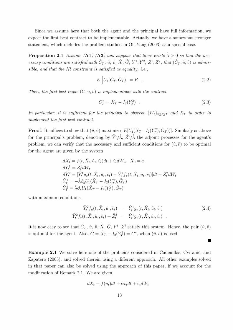
Since we assume here that both the agent and the principal have full information, we
expect the first best contract to be implementable. Actually, we have a somewhat stronger
statement, which includes the problem studied in Oh-Yang (2003) as a special case.
Proposition 2.1 Assume (A1)-(A3) and suppose that there exists λ > 0 so that the nec-
essary conditions are satisfied with CT , u, v, X, G, Y 1, Y 2, Z1, Z2, that (CT , u, v) is admis-
sible, and that the IR constraint is satisfied as equality, i.e.,
E[U1(CT , GT )
]= R . (2.2)
Then, the first best triple (C, u, v) is implementable with the contract
C∗T = XT − I2(Y 2T ) . (2.3)
In particular, it is sufficient for the principal to observe Wt0≤t≤T and XT in order to
implement the first best contract.
Proof: It suffices to show that (u, v) maximizes E[U1(XT−I2(Y 2T ), GT ))]. Similarly as above
for the principal’s problem, denoting by Y i/λ, Zi/λ the adjoint processes for the agent’s
problem, we can verify that the necessary and sufficient conditions for (u, v) to be optimal
for the agent are given by the system
dXt = f(t, Xt, ut, vt)dt+ vtdWt, X0 = x
dY 1t = Z1
t dWt
dY 2t = [Y 1
t gx(t, Xt, ut, vt)− Y 2t fx(t, Xt, ut, vt)]dt+ Z2
t dWt
Y 1T = −λ∂yU1(XT − I2(Y 2
T ), GT )
Y 2T = λ∂xU1(XT − I2(Y 2
T ), GT )
with maximum conditions
Y 2t fu(t, Xt, ut, vt) = Y 1
t gu(t, Xt, ut, vt) (2.4)
Y 2t fv(t, Xt, ut, vt) + Z2
t = Y 1t gv(t, Xt, ut, vt) .
It is now easy to see that CT , u, v, X, G, Y i, Zi satisfy this system. Hence, the pair (u, v)
is optimal for the agent. Also, C = XT − I2(Y 2T ) = C∗, when (u, v) is used.
Example 2.1 We solve here one of the problems considered in Cadenillas, Cvitanic, and
Zapatero (2003), and solved therein using a different approach. All other examples solved
in that paper can also be solved using the approach of this paper, if we account for the
modification of Remark 2.1. We are given
dXt = f(ut)dt+ αvtdt+ vtdWt
13

and GT =∫ T
0g(ut)dt, where W is one-dimensional. The agent’s utility is non-separable,
U1(x, y) = U1(x − y). We denote I1(z) := (U ′1)−1(z). The corresponding necessary and
sufficient conditions are
dXt = f(ut)dt+ αvt + vtdWt, X0 = x
dY 1t = Z1
t dWt, dY 2t = Z2
t dWt
Y 1T = Y 2
T = U ′2(XT − CT ) = λU ′1(CT − GT ) .
We see that Y 1 = Y 2, Z1 = Z2, so that the maximum conditions become
f ′(u) = g′(u), αY 1t = −Z1
t .
We assume that the first equality has a unique solution u (which is then constant). The
second equality gives Y 1t = zλ exp−1
2α2t− αWt for some z > 0, to be determined below.
The optimal contract should be of the form
CT = XT − I2(Y 1T ) = I1(Y 1
T /λ) + GT .
The value of z has to be chosen so that E[U1(I1(Y 1T /λ))] = R, assuming such a value z
exists. Denote Zt :=Y 1t
zλ. Then Z is a martingale with Z0 = 1. We have
d(ZtXt) = Zt[f(u)dt+ vtdWt]
so that ZtXt −∫ t
0Zsf(u)ds has to be a martingale. The above system of necessary and
sufficient conditions will have a solution if we can find v using the Martingale Representation
Theorem, where we now consider the equation for ZX as a Backward SDE having a terminal
condition
ZT XT = ZTI2(zλZT ) + I1(zZT ) + GT .
This BSDE has a solution which satisfies X0 = x if and only if there is a solution λ > 0 of
the equation
x = E[ZT XT ]− f(u)T = E[ZTI2(zλZT ) + I1(zZT ) + GT]− f(u)T .
This is indeed the case in examples with exponential utilities Ui(x) = − 1γie−γix, γi > 0,
solved in Cadenillas, Cvitanic, and Zapatero (2003). It is straightforward in this case to
check that the solution obtained by the method of this example is indeed admissible. The
same is true for power utilities, Ui(x) = 1γixγi , γi < 1, if we account for Remark 2.1.
3 Hidden action; the second best contracts
3.1 The model
We first recall (2.1). In the full information case, the principal observes X, u, v and W .
In the so-called hidden action case, the principal can only observe the controlled process
14

Xt, but not the underlying Brownian motion W or the agent’s control u (so the agent’s
”action” ut is hidden to the principal). We note that the principal observes the process X
continuously, which implies that the volatility control v can also be observed, through the
quadratic variation of X.
Under this framework, the contract CT can only depend on X (and v), but not on W
or u. So the first best contract obtained in Section 2, which may depend on W , may not
be feasible here. We note that, similarly as in Section 2, for a given process v, the principal
can write a contract to induce (or ”force”) the agent to implement it. In this sense, we may
consider v as a control chosen by the principal instead of by the agent. For simplicity, in this
section we assume v = 1. However, we note that all the results in this section, under certain
technical conditions and after some obvious modifications, hold true when v is controlled by
the principal. We provide the main results for this case in remarks below.
Another important assumption we make is that u depends on X, rather than W . That
is, for any t, ut is a (deterministic) mapping from C[0, t] to IR, and (2.1) becomes
dXt = f(t,Xt, ut(X·))dt+ dWt. (3.5)
This is common in the literature, and can be interpreted to mean that the agent chooses
his action based on the company’s performance up to current time. For simplicity, we abuse
the notation by writing ut = ut(X·) when there is no danger of confusion.
For any given contract CT = CT (X·), the agent’s problem is to find optimal u = uCT
such that V1(uCT ) = maxu V1(u) where
V1(u)4= EU1(CT , G
uT ), Gu
T
4=
∫ T
0
g(t,Xt, ut)dt
and X is the solution to (3.5). Denote the optimal X as XCT . Then the principal’s problem
is to find optimal CT so as to maximize V2(CT )4= EU2(XCT
T −CT ) under the IR constraint
V1(uCT ) ≥ R.
In this section we discuss only the case of separable utility for the agent U1(C,G) =
U1(C)−G (by abusing the notation U1). The non-separable case appears to be much harder
and is left for future research.
3.2 The agent’s problem
3.2.1 A weak formulation
Since we want to maximize expectations, a mathematically convenient way to model the
agent’s problem is to use the weak formulation, and this is standard in the literature. The
structure of (3.5) enables us to do so as follows. Let (C([0, T ]),G, Q) be the Wiener space, B
15

be the canonical Brownian Motion process, and G4= Gt0≤t≤T be the filtration generated
by B. Denote
X0t
4= x+Bt.
Then B is a Q-Brownian motion and by definition ut(X0· ) is a G-adapted process. For
notational simplicity, throughout §3.2 we abbreviate ut(X0· ) as ut. By Girsanov Theorem,
under some technical conditions, the process
But :4= Bt −
∫ t
0
f(s,X0s , us)ds
is a Brownian motion under probability Qu where dQu
dQ= Mu
T and Mut is the solution to the
following SDE:
dMut = Mu
t f(t,X0t , ut)dBt; Mu
0 = 1.
Note that
dX0t = dBt = f(t,X0
t , ut)dt+ dBut .
So (C([0, T ]),G, Qu,G, Bu, X0) is a weak solution to (3.5). Therefore, for any GT measurable
variable CT (X0· ), also abbreviated as CT ,
V1(u) = EQuU1(CT )−GuT = EQMu
T [U1(CT )−GuT ]. (3.6)
Throughout this section we write Eu 4= EQu and E4= EQ. For any p ≥ 1, denote
LpT (Qu)4= ξ ∈ GT : Eu|ξ|p <∞; Lp(Qu)
4= η ∈ G : Eu
∫ T
0
|ηt|pdt <∞,
and define LpT (Q), Lp(Q) in a similar way. We now fix CT ∈ GT such that E|U1(CT )|2 <∞.
We will impose the following assumptions:
(A5.) f, g are continuously differentiable with respect to x, u, fugu > 0, f is concave in
u and g is convex in u.
(A6.) The admissible set A(CT ) of agent’s controls is the set of all those u ∈ G such
that
(i) U1(CT )−GT ∈ L4(Qu);
(ii) [MuT ]−1 ∈ L2(Q);
(iii) for any bounded ∆u ∈ G, there exists ε0 > 0 such that for any ε ∈ [0, ε0],
|f ε|8, |f εu|8, |gε|2, |gεu|2, |M εT |4 are uniformly integrable in L1(Q) or L1
T (Q), where
uε4= u+ ε∆u, Gε
t
4= Guε
t , M εt
4= Muε
t , V ε1
4= V1(uε),
16

and
f ε(t)4= f(t,X0
t , uεt), f εu(t)
4= fu(t,X
0t , u
εt), gε(t)
4= g(t,X0
t , uεt), gεu(t)
4= gu(t,X
0t , u
εt),
When ε = 0 we omit the superscript “0”. By (A6)(iii), one can easily show that
supε∈[0,ε0]
E∫ T
0
[|f ε(t)|8 + |f εu(t)|8 + |gε(t)|2 + |gεu(t)|2]dt+ |GεT |2 + |M ε
T |4<∞; (3.7)
and
limε→0
E∫ T
0
[|f ε(t)−f(t)|8+|f εu(t)−fu(t)|8+|gε(t)−g(t)|2]dt+|GεT−GT |2+|M ε
T−MT |4
= 0.
(3.8)
3.2.2 Necessary and sufficient conditions
Now we fix CT and u ∈ A(CT ). Denote
∇f(t)4= fu(t,X
0t , ut)∆ut; ∇g(t)
4= gu(t,X
0t , ut)∆ut;
∇Gt4=
∫ t
0
∇g(s)ds; ∇Mt4= Mt[
∫ t
0
∇f(s)dBs −∫ t
0
f(s)∇fsds];
∇V14= E∇MT [U1(CT )−GT ]−MT∇GT.
Moreover, for any bounded ∆u ∈ G and ε ∈ (0, ε0] as in (A6)(iii), denote
∇f ε(t) 4= f ε(t)− f(t)
ε; ∇gε(t) 4= gε(t)− g(t)
ε;
∇GεT
4=GεT −GT
ε; ∇M ε
T
4=M ε
T −MT
ε; ∇V ε
1
4=V ε
1 − V1
ε.
Lemma 3.1 Assume (A5), (A6). Then
limε→0
E∫ T
0
[|∇f ε(t)−∇f(t)|8 + |∇gε(t)−∇g(t)|2]dt+ |∇GεT−∇GT |2 + |∇M ε
T−∇MT |2
= 0.
Proof. First, note that ∇f ε(t) =
∫ 1
0
f δεu (t)dδ∆ut. Then
|∇f ε(t)−∇f(t)| ≤∫ 1
0
|f δεu (t)− fu(t)|dδ|∆ut|.
By (3.8) we get
limε→0
E∫ T
0
|∇f ε(t)−∇f(t)|8dt
= 0. (3.9)
17

Similarly,
limε→0
E∫ T
0
|∇gε(t)−∇g(t)|2dt
= 0; limε→0
E|∇GεT −∇GT |2 = 0.
Second, noting that M εT = exp(
∫ T0f ε(t)dBt − 1
2
∫ T0|f ε(t)|2dt) we have
∇M εT =
∫ 1
0
M δεT [
∫ T
0
∇f δε(t)dBt −∫ T
0
f δε(t)∇f δε(t)dt]dδ.
Then
E|∇M εT −∇MT |2 = E
∣∣∣∫ 1
0
[(M δε
T
∫ T
0
∇f δε(t)dBt −MT
∫ T
0
∇f(t)dBt
)
−(M δε
T
∫ T
0
f δε(t)∇f δε(t)dt−MT
∫ T
0
f(t)∇f(t)ds)]dδ∣∣∣2
≤ C
∫ 1
0
E|M δε
T −MT |2|∫ T
0
∇f δε(t)dBt|2 + |MT |2|∫ T
0
[∇f δε(t)−∇f(t)]dBt|2
+|M δεT −MT |2|
∫ T
0
f δε(t)∇f δε(t)dt|2
+|MT |2|∫ T
0
[(f δε(t)− f(t))∇f δε(t) + f(t)(∇f δε(t)−∇f(t))]dt|2dδ
≤ C
∫ 1
0
[√E|M δε
T −MT |4√E∫ T
0
|∇f δε(t)|4dt
+√E|MT |4
√E∫ T
0
|∇f δε(t)−∇f(t)|4dt
+√E|M δε
T −MT |4[∫ T
0
E|f δε(t)|8dt] 14 [
∫ T
0
E|∇f δε(t)|8dt] 14
+√E|MT |4[
∫ T
0
E|f δε(t)− f(t)|8dt] 14 [
∫ T
0
E|∇f δε(t)|8dt] 14
+√E|MT |4[
∫ T
0
E|f(t)|8dt] 14 [
∫ T
0
E|∇f δε(t)−∇f(t)|8dt] 14
]dδ
≤ C
∫ 1
0
[√E|M δε
T −MT |4+
√E∫ T
0
|∇f δε(t)−∇f(t)|4dt
+[
∫ T
0
E|f δε(t)− f(t)|8dt] 14 + [
∫ T
0
E|∇f δε(t)−∇f(t)|8dt] 14
]dδ,
thanks to (3.7). Then by (3.8) and (3.9) we prove the result.
Corollary 3.1 Assume (A5), (A6). Then
limε→0
V ε1 = V1; lim
ε→0∇V ε
1 = ∇V1.
18

Proof. The first equality is obvious. We prove only the second one. Noting that
∇V ε1 = E
∇M ε
T [U1(CT )−GT ]−M εT∇Gε
T
,
we have
|∇V ε1 −∇V1| =
∣∣∣E
[∇M εT −∇MT ][U1(CT )−GT ]− [M ε
T∇GεT −MT∇GT ]
∣∣∣≤ E
|∇M ε
T −∇MT ||U1(CT )−GT |+ |M εT −MT ||∇GT |+ |M ε
T ||∇GεT −∇GT |
≤√E|∇M ε
T −∇MT |2√E|U1(CT )−GT |2
+√E|M ε
T −MT |2√E|∇GT |2+
√E|M ε
T |2√E|∇Gε
T −∇GT |2
≤ C[√
E|∇M εT −∇MT |2+
√E|M ε
T −MT |2+√E|∇Gε
T −∇GT |2],
thanks to (A6). Then by (3.8) and Lemma 3.1 we prove the result.
We next introduce the adjoint processes. By (A6)(i), Eu|U1(CT )−GT |4 <∞, so, by
the BSDE theory, there exists a unique solution (Y 0t , Z
0t ) to the BSDE
Y 0t = [U1(CT )−GT ]−
∫ T
t
Z0sdB
us . (3.10)
such that
Eu
sup0≤t≤T
|Y 0t |4 + [
∫ T
0
|Z0t |2dt]2
<∞. (3.11)
Lemma 3.2 Assume (A5), (A6). Then
∇V1 = Eu∫ T
0
[Z0t fu(t)− gu(t)]∆utdt
.
Proof: Applying Ito’s formula we have
∇V1 = Eu∇MT
MT
Y 0T −∇GT
= Eu
∫ T
0
[Z0t fu(t)− gu(t)]∆utdt+
∫ T
0
ΛtdBut
,
where
Λt = Y 0t fu(t)∆ut +
∇Mt
Mt
Z0t
We have, by continuity and definition of Z0t ,
sup0≤t≤T
[|Y 0t |2 +
|∇Mt|2M2
t
] +
∫ T
0
[|Z0t |2 + |fu(t)|2]dt <∞ a.s.
19
therefore∫ T
0|Λt|2dt <∞, a.s. Noting that ∇Mt
Mt=∫ T
0∇f(t)dBu
t we get
Eu
sup0≤t≤T
∣∣∣∇Mt
Mt
Y 0t −∇Gt
∣∣∣≤ CEu
[sup
0≤t≤T
|Y 0t |2 + |∇Gt|+ |
∫ t
0
fu(t)∆utdBut |2]
≤ C + CEu∫ T
0
[|gu(t)|+ |fu(t)|2]dt
= C + CEMT
∫ T
0
[|gu(t)|+ |fu(t)|2]dt
≤ C + CEM2
T +
∫ T
0
[|gu(t)|2 + |fu(t)|4|]dt<∞,
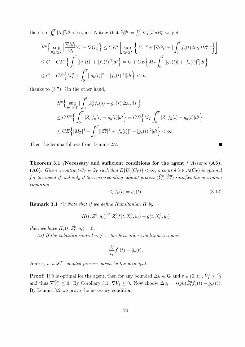
thanks to (3.7). On the other hand,
Eu
sup0≤t≤T
|∫ t
0
[Z0sfu(s)− gu(s)]∆usds|
≤ CEu∫ T
0
|Z0t fu(t)− gu(t)|dt
= CE
MT
∫ T
0
|Z0t fu(t)− gu(t)|dt
≤ CE|MT |4 +
∫ T
0
[|Z0t |2 + |fu(t)|4 + |gu(t)|2]dt
<∞
Then the lemma follows from Lemma 2.2.
Theorem 3.1 (Necessary and sufficient conditions for the agent.) Assume (A5),
(A6). Given a contract CT ∈ GT such that EU1(CT ) <∞, a control u ∈ A(CT ) is optimal
for the agent if and only if the corresponding adjoint process (Y 0t , Z
0t ) satisfies the maximum
condition
Z0t fu(t) = gu(t). (3.12)
Remark 3.1 (i) Note that if we define Hamiltonian H by
H(t, Z0, ut)4= Z0
t f(t,X0t , ut)− g(t,X0
t , ut)
then we have Hu(t, Z0t , ut) = 0.
(ii) If the volatility control vt 6= 1, the first order condition becomes
Z0t
vtfu(t) = gu(t).
Here vt is a FXt -adapted process, given by the principal.
Proof: If u is optimal for the agent, then for any bounded ∆u ∈ G and ε ∈ (0, ε0], V ε1 ≤ V1
and thus ∇V ε1 ≤ 0. By Corollary 3.1, ∇V1 ≤ 0. Now choose ∆ut = sign(Z0
t fu(t) − gu(t)).By Lemma 3.2 we prove the necessary condition.
20

As for sufficiency, assume u ∈ A satisfies (3.12). For any u ∈ A, noting that EuY 0T is
a (deterministic) constant we have
EuY 0T = EuEuY 0
T = EuY 0T −
∫ T
0
Z0t dB
ut .
Thus
V1(u)− V1(u) = EuY 0T − EuY 0
T + GT −GT
= −Eu∫ T
0
Z0t dB
u + GT −GT
= −Eu
∫ T
0
Z0t dB
ut −
∫ T
0
Z0t [f(t)− f(t)]dt+ GT −GT
.
By (3.11) and (A6)(ii), (iii) we have
Eu∫ T
0
|Z0t |2dt
= Eu
MT
MT
∫ T
0
|Z0t |2dt
≤ Eu
|MT |2|MT |2
+ E
[
∫ T
0
|Z0t |2dt]2
≤ C + E |MT |2MT
≤ C + E|MT |4+ E|MT |−2 <∞,
which implies that Eu∫ T0Z0t dB
ut = 0. Thus
V1(u)− V1(u) = Eu
[∫ T
0
(H(t, Z0t , ut)−H(t, Z0
t , ut))dt
]
By the maximum condition (3.12) and (A5), the process Z0t is positive and H(t, z, u) is a
concave function of u that is maximal at u, and we obtain V1(u)− V1(u) ≥ 0 and finish the
proof.
We next show that the maximum condition (3.12) can be characterized by a BSDE. Re-
calling (A5), note that ∂u(gufu
) =guufu − fuugu
f 2u
which is always positive or always negative
depending on the sign of fu (and gu). Then for any x, z, the equation
zfu(t, x, u) = gu(t, x, u)
has a unique solution u = F (t, x, z). Recall that
Y 0t = U1(CT ) +
∫ T
0
g(s,Xs, us)ds−∫ T
t
Z0t dBs +
∫ T
t
f(s,Xs, us)ds
Therefore, by denoting
Kt4= Y 0
t −∫ t
0
g(s,Xs, us)ds (3.13)
we get
Kt = U1(CT ) +
∫ T
t
[f + g](s,Xs, F (s,Xs, Z0s ))ds−
∫ T
t
Z0t dBs. (3.14)
The following theorem is obvious now.
21

Theorem 3.2 Assume (A5), (A6). If u ∈ A is optimal for the agent, then (K, Z0)
defined as above is the solution to the BSDE (3.14). On the other hand, if BSDE (3.14) has
a solution (K, Z0) such that ut4= F (t,Xt, Z
0t ) ∈ A(CT ), then u is the optimal control for
the agent.
Finally we note that if [f + g](t, x, F (t, x, z)) is uniformly Lipschitz continuous on z and
E∫ T0|[f+g](t,Xt, F (t,Xt, 0))|2dt <∞, then BSDE (3.14) has a unique solution, and thus
the agent’s problem has a unique optimal control.
3.2.3 Implementable contracts
Suppose that given a contract CT the agent optimally implements the control u. Then, from
the necessary conditions we get
CT = J1(Y 0T +
∫ T
0
g(t)dt) (3.15)
where J1 = U−11 . From the maximum condition (3.12) and BSDE (3.10), we get
Z0t =
gu(t)
fu(t); Y 0
t = Y 00 −
∫ t
0
gu(s)
fu(s)f(s)ds+
∫ t
0
gu(s)
fu(s)dBs. (3.16)
For any number Y 00 , the pair (Y 0
t , Z0t ) satisfies the necessary and sufficient conditions of the
agent’s problem with CT as in (3.15), so the agent will choose the action u. Thus, we have
Corollary 3.2 Under the conditions of this section, the control u is implementable by CT
if and only if (3.15) and (3.16) are satisfied. In addition, the optimal utility of the agent
under this contract is V1(u) = Y 00 .
Remark: In general, it is known that the agent’s first order conditions are not sufficient to
characterize implementable contracts. In other words, the set of implementable contracts
may be smaller than the set given by the first order conditions. Here, we have found condi-
tions under which these two sets are equal, and under which the contract that implements
a given action u is unique. This was also done in Williams (2004) in a somewhat different
framework and under stronger assumptions.
3.3 The principal’s problem
3.3.1 The relaxed principal’s problem
To investigate the principal’s problem, for technical reasons we use the strong formulation
(3.5). To this end, we shall first interpret the results in §3.2 under the strong formulation.
22

Recall that in §3.2 we denote ut(X0· ) by ut, which is Gt−measurable, and we denote CT (X0
· )
by CT , which is GT -measurable. Now assume u is a control such that (3.5) has a strong
solution X ∈ F. For any constant Y 10 , define
h(t, x, u)4=gu(t, x, u)
fu(t, x, u); Y 1
t
4= Y 1
0 +
∫ t
0
h(s,Xs, us(X·))dWs+
∫ t
0
g(s,Xs, us(X·))ds. (3.17)
Here, for simplicity, we work with Y 1t = Y 0
t +∫ t
0g(s), rather than with Y 0
t , as in §3.2. Note
that for given u, FX = F, thus there exists a contract CT such that
CT (X·) = J1(Y 1T ). (3.18)
By §3.2.3, under this contract, u is the optimal control by the agent and Y 10 is the agent’s
optimal utility. Equivalently to choosing the optimal contract, the principal may choose
optimal u and Y 10 so as to maximize her utility. Moreover, recalling the IR constraint (2.2),
one should have Y 10 ≥ R. It is easy to see then that it cannot be optimal for the principal
to choose Y 10 > R, and thus we can take Y 1
0 = R. Therefore, the principal’s problem is
maxu
V2(u)4= max
uEPU2(XT − CT ) (3.19)
where XT is the solution to (3.5), CT is defined by (3.18), and Y 1 is defined by
dY 1t = h(t,Xt, ut(X·))dWt + g(t,Xt, ut(X·))dt, Y 1
0 = R. (3.20)
We assume that the principal can choose only those u such that (3.5) has a strong solution
X ∈ F.
In order to use the strong formulation, we first study the following so-called relaxed
principal’s problem:
maxu
V2(u)4= max
uEPU2(XT − CT ), (3.21)
where u is F-adapted, CT = J1(Y 1T ), and
dXt = f(t,Xt, ut)dt+ dWt, X0 = x;
dY 1t
4= h(t,Xt, ut)dWt + g(t,Xt, ut)dt; Y 1
0 = R.(3.22)
We note that, for notational simplicity, here we use the same notations u,X, Y 1 and V2 as
in the previous paragraph. In this subsection and §3.3.2 we will consider only the relaxed
principal’s problem, and we will distinguish these notations when we come back to the (non-
relaxed) principal’s problem in §3.3.3. We denote EP as E (note that in §3.2 E is a notation
for EQ). We impose the following assumptions for the relaxed principal’s problem:
(A7.) (A1), (A2) hold true (by removing the v part in the obvious way); fugu > 0; and h
is continuously differentiable in (x, u) such that hx is uniformly bounded and hu has uniform
linear growth in (x, u).
23

(A8.) The admissible set A of control u is the set of all those u ∈ F such that
(i) E∫ T0
[|ut|2 + |f(t, 0, ut)|2 + |h(t, 0, ut)|2]dt <∞;
(ii) E|U ′2(XT − CT )|4 + |J ′1(Y 1T )|4 <∞;
(iii) for any bounded ∆u ∈ F, there exists ε0 > 0 (which may be different from the
ε0 in (A6)) such that for any ε ∈ [0, ε0], uε4= u + ε∆u satisfies (i),(ii) and |U ′2(Xε
T −CεT )|4, |J ′1(Y 1,ε
T )|4 are uniformly integrable, where CεT
4= J1(Y 1,ε
T ), and
dXε
t = f(t,Xεt , u
εt)dt+ dWt, Xε
0 = x;
dY 1,εt = g(t,Xε
t , uεt)dt+ h(t,Xε
t , uεt)dWt, Y 1,ε
0 = R.
We note that (A7) implies (A5); and (A7) and (A8)(i) implies that (3.22) has unique
strong solutions.
3.3.2 Necessary and sufficient conditions
Denote f(t)4= f(t,Xt, ut), f
ε(t)4= f(t,Xε
t , uεt), and other terms in a similar way. Define
d∇Xt = [fx(t)∇Xt + fu(t)∆ut]dt, ∇X0 = 0;
d∇Y 1t = [gx(t)∇Xt + gu(t)∆ut]dt+ [hx(t)∇Xt + hu(t)∆ut]dWt, ∇Y 1
0 = 0;
∇V24= EU ′2(XT − CT )∇XT − U ′2(XT − CT )J ′1(Y 1
T )∇Y 1T .
We further define ∇Xεt
4=
Xεt−Xtε
and other finite difference quotient terms in a similar way.
By the same techniques as in Section 2 (or §3.2) one can prove
Lemma 3.3 Assume (A7), (A8). Then
E
sup0≤t≤T
[|Xt|2 + |∇Xt|2 + |Y 1t |2 + |∇Y 1
t |2]<∞;
limε→0
E
sup0≤t≤T
[|Xε
t −Xt|2 + |∇Xεt −∇Xt|2 + |∇Y 1,ε
t −∇Y 1t |2]
= 0;
limε→0
V ε2 = V2; lim
ε→0∇V ε
2 = ∇V2.
We now define two adjoint processes:
Y 2t = U ′2(XT − CT ) +
∫ Tt
[Y 2s fx(t)− Y 3
s gx(t)− Z3shx(t)]ds−
∫ TtZ2sdWs;
Y 3t = U ′2(XT − CT )J ′1(Y 1
T )− ∫ TtZ3sdWs.
By our assumptions, there exist unique solutions (Y 2t , Z
2t ), (Y 2
t , Z3t ), such that
E
sup0≤t≤T
[|Y 2t |2 + |Y 3
t |2] +
∫ T
0
[|Z2t |2 + |Z3
t |2]dt<∞.
We now have
24

Lemma 3.4 Assume (A7), (A8). Then
∇V2 = E∫ T
0
Γt∆utdt,
where
Γt4= Y 2
t fu(t)− Y 3t gu(t)− Z3
t hu(t).
Proof: Using Ito’s rule , we have
∇V2 = EY 2T∇XT − Y 3
T∇Y 1T
= E
∫ T
0
Γt∆utdt+
∫ T
0
γtdWt
where
γt = ∇XtZ2t +∇Y 1
t Z3t − Y 3
t hx(t)∇Xt − Y 3t hu(t)∆ut
As before, we can check by Lemma 3.3 that∫ T
0|γt|2dt <∞ a.s., and that
E
[sup
0≤t≤T
∣∣Y 2t ∇Xt − Y 3
t ∇Y 1t
∣∣]<∞; E
∫ T
0
|Γt∆ut|dt<∞,
which completes the proof, using Lemma 2.2.
The main result of this section is the following theorem whose proof is similar as above
and thus is omitted.
Theorem 3.3 (Necessary Condition of Optimality with Hidden Action) Assume
(A7), (A8). If u ∈ A is the optimal solution for the relaxed principal’s problem, the
following maximum condition holds true:
Γt = 0. (3.23)
Remark 3.2 (i) If the principal can also control volatility vt, the first order condition of
the principal ’s relaxed problem becomes
Γt = 0, Γvt = 0
where
Γvt4= Y 2
t fv(t)− Y 3t gv(t)− Z3
t hv(t) + Z2t
(ii) If we define the Hamiltonian by
H(t, Y, Z, u, v,X) = Y 2t f(t,Xt, u, v)− Y 3
t g(t,Xt, u, v)− Z3t h(t,Xt, u, v) + Z2
t vt
the first order condition, if v is not controlled, is equivalent to
∂uH(t, Y, Z, u, v,X) = 0;
and if v is controlled, in addition we have
∂vH(t, Y, Z, u, v,X) = 0
25

If there exists a unique one-to-one function F (t,X, Y, Z),, such that
∂uH(t, Y, Z, F1(t,X, Y, Z), X) = 0 so that ut = F (t,X, Y, Z), then the necessary conditions
can be written as a system of fully coupled Backward-Forward SDEs.
We also have a sufficient condition for the optimality:
Theorem 3.4 (Sufficient Conditions for the Principal) Assume (A7), (A8). If
H(t, Y, Z, u,X) is jointly concave in (X, u) for any (Y, Z), then the control u ∈ A satis-
fying the maximum condition (3.23) is optimal for the relaxed principal’s problem.
Proof: Take any u ∈ A. By concavity of U2 and −J1, and U ′2 < 0, suppressing the
arguments we get
V2(u)− V2(u) = EU2(XT − CT )− U2(XT − CT )
≥ EU ′2[XT −XT ]− U ′2[J1(Y 1
T )− J1(Y 1T )]
≥ EU ′2[XT −XT ]− U ′2J ′1[Y 1
T − Y 1T ]
≥ EY 2T [XT −XT ]− Y 3
T
[ ∫ T
0
[h(t)− h(t)]dWt +
∫ T
0
[g(t)− g(t)]dt].
Using Ito’s rule and then applying Lemma 2.2 we get
V2(u)− V2(u) ≥ E∫ T
0
[Y 2t [f(t)− f(t)] + [Xt −Xt][Y
1t fx(t)− Y 3
t gx(t)− Z3t hx(t)]
+Y 3t [g(t)− g(t)] + Z3
t [h(t)− h(t)]]dt
= E∫ T
0
[H(t, Xt, Yt, Zt, ut)−H(t,Xt, Yt, Zt, ut)− [Xt −Xt]Hx(t, Xt, Yt, Zt, ut)
]dt
≥ 0,
which completes the proof.
3.3.3 The principal’s problem
We now come back to the principal’s problem (3.19). In order to avoid notational confusion,
we take the convention that all the terms related to the relaxed principal’s problem have
the superscript . For example, while u denotes a control for the principal’s problem, we use
u ∈ F to denote a control in the relaxed principal’s problem.
We first note that, maxu
V2(u) ≤ maxu
V2(u). In fact, for any action u such that (3.5) has
a strong solution X, obviously ut4= ut(X·) is F-adapted. Thus V2(u) = V2(u) ≤ max
uV2(u).
On the other hand, if the conditions in Theorem 3.4 hold true, then the relaxed principal’s
problem has an optimal control ˆu. Let ˆX denote the diffusion corresponding to ˆu. If ˆu is
26

F ˆX-adapted, then there exists an action u such that ˆu = ut(ˆX ·) and ˆX is the strong solution
to (3.5) corresponding to u. Therefore,
maxu
V2(u) = V2(ˆu) = V2(u) ≤ maxu
V2(u).
The following lemma is obvious now.
Lemma 3.5 The following three statements are equivalent:
(i) maxu
V2(u) = maxu
V2(u); (ii) ˆu is F ˆX-adapted; (iii) W is F ˆX-adapted.
Moreover, if one of them holds true, then the u constructed above is the optimal control of
the principal’s problem (3.19). We note that in many examples, ˆu is deterministic, or even
constant, thus Lemma 3.5 (ii) holds true.
Our main result is the following theorem.
Theorem 3.5 Assume all the results in Theorem 3.4 hold true. Assume further that ˆu is
F ˆX-adapted and that u ∈ A(CT ), where the notations are defined in the obvious way. Then
CT is the optimal contract of the principal and u is the optimal action of the agent which is
implemented by CT .
3.4 Examples
Example 3.2 Let us consider the model
dXt = f(t, ut)dt+ dWt
with U1(x) = U2(x) = x, that is, both the principal and the agent are risk neutral. The
cost function is g(t, ut). Assume that f(t, ut) and −g(t, ut) are jointly concave in ut. The
necessary and sufficient conditions are
dXt = f(t, ut)dt+ dWt, X0 = x;
dY 1t = gu(t,ut)
fu(t,ut)dWt, Y 1
0 = R;
Y 2t ≡ Y 3
t ≡ 1, Z2t ≡ Z3
t ≡ 0
CT = Y 1T + GT
H(t, ut) = f(t, ut)− g(t, ut), ∂uH(t, ut) = 0
Assume that there exists a unique solution ut of the last equation, which is then a determin-
istic processes. The optimal contract is
CT = R +
∫ T
0
g(t, ut)dt+
∫ T
0
gu(t, ut)
fu(t, ut)dWt
which is equivalent to
CT = R +
∫ T
0
g(t, ut)dt−∫ T
0
f(t, ut)dt+
∫ T
0
gu(t, ut)
fu(t, ut)dXt
Note that if fu, gu are not functions of t, then the contract is linear in XT .
27
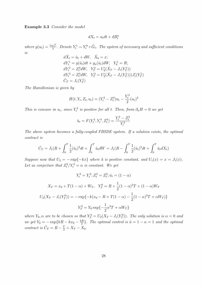
Example 3.3 Consider the model
dXt = utdt+ dBut
where g(ut) = (ut)2
2. Denote Y 1
t = Y 0t +Gt. The system of necessary and sufficient conditions
isdXt = ut + dW, X0 = x;
dY 1t = g(ut)dt+ gu(ut)dW, Y 1
0 = R;
dY 2t = Z2
t dW, Y 2T = U ′2(XT − J1(Y 1
T ))
dY 3t = Z3
t dW, Y 3T = U ′2(XT − J1(Y 1
T )))J ′1(Y 1T )
CT = J1(Y 1T )
The Hamiltonian is given by
H(t, Yt, Zt, ut) = (Y 2t − Z3
t )ut − Y 3t
2(ut)
2
This is concave in ut, since Y 3t is positive for all t. Then, from ∂uH = 0 we get
ut = F (Y 2t , Y
3t , Z
3t ) =
Y 2t − Z3
t
Y 3t
The above system becomes a fully-coupled FBSDE system. If a solution exists, the optimal
contract is
CT = J1(R +
∫ T
0
1
2(ut)
2dt+
∫ T
0
utdW = J1(R−∫ T
0
1
2(ut)
2dt+
∫ T
0
utdXt)
Suppose now that U2 = − exp−kx where k is positive constant, and U1(x) = x = J1(x).
Let us conjecture that Z3t /Y
3t = α is constant. We get
Y 3t = Y 2
t ;Z3t = Z2
t ; ut = (1− α)
XT = x0 + T (1− α) +WT , Y 0T = R +
1
2(1− α)2T + (1− α)WT
U2(XT − J1(Y 0T )) = − exp−k(x0 −R + T (1− α)− 1
2(1− α)2T + αWT )
Y 3T = Y0 exp−1
2α2T + αWT
where Y0, α are to be chosen so that Y 3T = U2(XT − J1(Y 0
T )). The only solution is α = 0 and
we get Y0 = − expkR − kx0 − kR2. The optimal control is u = 1− α = 1 and the optimal
contract is CT = R− T2
+XT −X0.
28

3.5 Non-separable utility; Original Holmstrom-Milgrom problem
We can write down the conjectured necessary and sufficient conditions for the non-separable
case U1(CT −GT ), but we have been unable to provide the complete proofs, which we leave
for future research. We sketch here how the approach of this paper still works in the original
Holmstrom-Milgrom problem, due to its special structure.
Similarly as above, we can prove that the necessary conditions for the agent are
dMt = Mtf(t,X0t , ut)dBt, M0 = 1
dY 1t = Z1
t dBut , Y 1
T = U ′1(CT − GT )
dY 2t = Z2
t dBut , Y 2
T = U1(CT − GT )
with maximum condition
Z2t fu(ut) = Ytgu(ut).
We see that Y iM is a P−martingale. Therefore,
E[Y 2TMT ] = E[MTU1(CT − GT )] = R = Y 2
0 M0 = Y 20 .
We also have CT − GT = J1(Y 2T ) where J1 = U−1
1 . Thus, we get
MtY1t = Et[MTU
′1(CT − GT )] = Et[MTU
′1(J1(Y 2
T ))]
Then, by using the maximum condition to find Z2, we have
dY 2 = Z2dBu = Y 1 guMfu
dBu = Et[MTU′1(J1(Y 2
T ))]gufudBu (3.24)
with initial condition Y 20 = R. We recall the Holmstrom and Milgrom (1987) setting, where
only the drift is controlled,
dXt = f(ut)dt+ dBut
For simplicity of notation we consider only the one-dimensional case, withB a one-dimensional
Brownian Motion. Moreover, we assume
Ui(x) = −e−γix, g(u) = u2/2, f(u) = u.
Then,
J1(y) = − log(−y)/γ1, U ′1(x) = γ1e−γ1x, fu = 1
Since MY 2 is a P−martingale, we get, from (3.24),
dY 2 = −γ1Et[MTY2T ]ut/MtdB
u = −γ1Y2t utdB
ut
or
Y 2t = Re−
R t0 γ
21 u
2t /2dt−
R t0 γ1utdBut
29

The principal’s problem is to maximize
Eu[U2(XT − J1(Y 2T (u))−GT )] (3.25)
If we plug Y 2 into this expression with the exponential function U2, we get that we need to
minimize
Eu
[exp
−γ2
(X0 +
∫ T
0
utdt+BuT +
1
γ1
[log(−R)− 1
2
∫ T
0
γ21u
2tdt−
∫ T
0
γ1utdBut
]−∫ T
0
u2t
2dt
)].
This is a simple and known stochastic control problem (which can be solved by HJB equa-
tion), the solution of which is constant u, the same as in Holmstrom-Milgrom (1987), and
given by
u =1 + γ2
1 + γ1 + γ2
The optimal contract is linear, and given by f(XT ) = a+ bXT , where b = u and a is chosen
so that the IR constraint is satisfied,
a = − 1
γ1
log(−γ1R)− bS0 +b2T
2(γ1 − 1) . (3.26)
4 Conclusions
We have built a fairly general theory for Principal-Agent problems in models driven by
Brownian Motion. A question still remains under which general conditions the optimal con-
tract exists. The recent most popular application is the optimal compensation of executives.
In order to have more realistic framework for that application, other forms of compensation
should be considered, such as a possibility for the agent to cash in the contract at a random
time. We leave these problems for future research.
30

References
[1] A. Cadenillas, J. Cvitanic and F. Zapatero, “ Dynamic Principal-Agent problems with
perfect information”. Working paper, University of Southern California (2003).
[2] J. Detemple, S. Govindaraj, M. Loewenstein, Optimal Contracts and Intertemporal
Incentives with Hidden Actions, working paper, Boston University, (2001).
[3] B. Holmstrom and P. Milgrom, “Aggregation and Linearity in the Provision of In-
tertemporal Incentives”, Econometrica 55 (1987), 303–328.
[4] D. G. Luenberger, Optimization by Vector Space Methods. Wiley-Interscience, (1997).
[5] J. Ma, and J. Yong, Forward-Backward Stochastic Differential Equations and Their
Applications. Lecture Notes in Math. 1702. Springer, Berlin, (1999).
[6] H. Ou-Yang, “Optimal Contracts in a Continuous-Time Delegated Portfolio Manage-
ment Problem”, Review of Financial Studies 16 (2003), 173–208.
[7] H. Schattler and J. Sung, “The First-Order Approach to the Continuous-Time
Principal-Agent Problem with Exponential Utility”, J. of Economic Theory 61 (1993),
331–371.
[8] J. Sung, “Lectures on the theory of contracts in corporate finance”, preprint, University
of Illinois at Chicago (2001).
[9] J. Sung, “Linearity with project selection and controllable diffusion rate in continuous-
time principal-agent problems”, RAND J. of Economics 26 (1995), 720–743.
[10] N. Williams, ”On Dynamic Principal-Agent Problems in Continuous Time”. Working
paper, Princeton University, (2004).
[11] J. Yong, “Completeness of Security Markets and Solvability of Linear Backward
Stochastic Dierential Equations”. Working paper, University of Central Florida, (2004).
[12] J. Yong and X.Y. Zhou, “Stochastic Controls: Hamiltonian Systems and HJB Equa-
tions,” Springer-Verlag, New York, (1999).
31