Continuous-Time State Space Analysis

Continuous-Time State Space Analysis

Thestatespacemodelof a continuous-timelinearsystemis representedby a system

of linear differential equations.In matrix form, it is given by �wherethe vectors

�,

�, and

�are, respectively,the

statevector, input vector, and output vector, that is��...�

��...�

��...�

We call the dimensionof the system, the dimensionof the systeminput and

the dimensionof the systemoutput.

The slides contain the copyrighted material from Linear Dynamic Systems and Signals, Prentice Hall 2003. Prepared by Professor Zoran Gajic 8–1

The matrix��

describesthe internal behaviorof the system,while matrices��,

��, and

��representconnectionsbetweentheexternalworld andthe

system.If thereareno direct pathsbetweeninputsandoutputs,which is often the

case,the matrix ��

is zero.

Thesematricesrepresentarraysof real scalarnumbersas�� ...... ...� � �� ...

... ...� � �� ...

... ... � �� ...... ... � ��

It is assumedin this book that all matricesare time invariant, which implies that

all scalars �� and �� are constant.


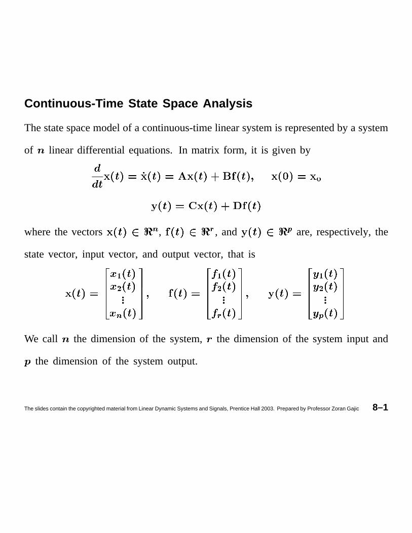
In the next sectionwe will showhow to relatedifferentialequationsdescribing

linear dynamicalsystemsto the statespaceform, and show how to determine,in

general,scalars �� . In this chapter,we will encountermathematical

models of electrical networks, electrical machines,aircraft, antennas,industrial

reactors,robots,describedby statespaceforms.

Note that the statespacemodel for linear discrete-timesystemshasexactly the

sameform with the vector differential equationreplacedby the vector difference

equations � � � �In the next two exampleswe demonstratehow to obtain statespaceforms for

two standardelectricaland mechanicallinear systems.


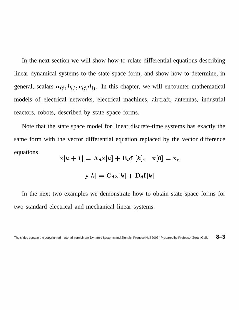
Example 8.1: Considera simple RLC electricalnetwork given in Figure 1.10

of Section 1.3, whose mathematicalmodel is representedby the second-order

differential equation,that is! " ! # !! " # !! " $In this mathematicalmodel

$representsthe systeminput and

"is the

systemoutput. Introducingthe following changeof variables# % # % !! %$% #


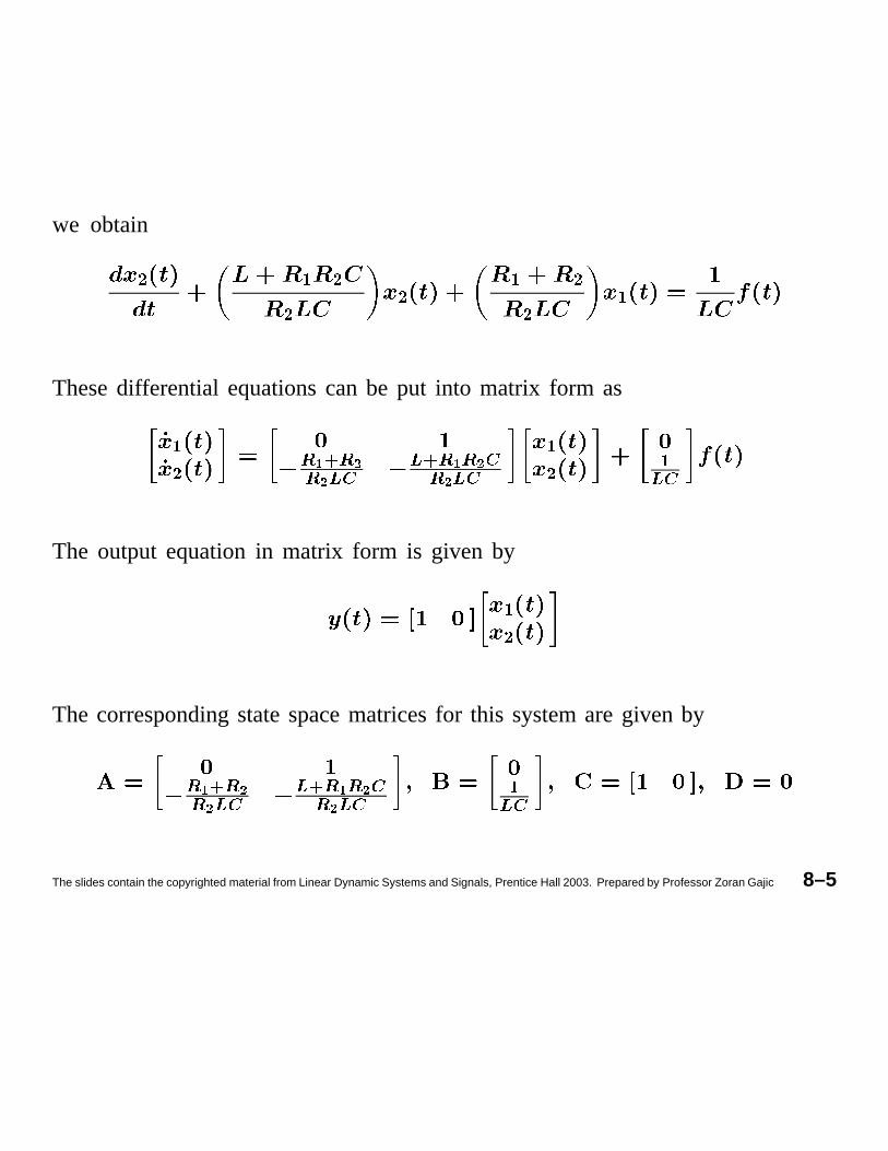
we obtain& ' && & ' && 'Thesedifferential equationscan be put into matrix form as'& (*),+�(.-(/-10�2 03+�(*)4(.-52(.-,0�2 '& '0�2The output equationin matrix form is given by'&The correspondingstatespacematricesfor this systemare given by

(*)6+.(.-( - 032 0�+.(*)4(.-52( - 0�2 '0�2The slides contain the copyrighted material from Linear Dynamic Systems and Signals, Prentice Hall 2003. Prepared by Professor Zoran Gajic 8–5

Thestatespaceformof a systemis notunique. Usinganotherchangeof variables,

we canobtain, for the samesystem,anotherstatespaceform (as demonstratedin

Problem8.1). This issuewill be further clarified in Section8.4.

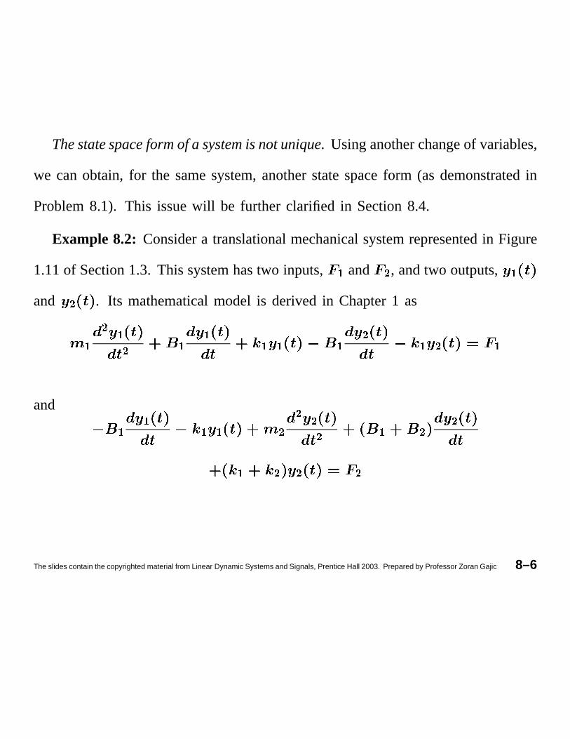
Example 8.2: Considera translationalmechanicalsystemrepresentedin Figure

1.11of Section1.3. This systemhastwo inputs, 7 and 8 , andtwo outputs, 7and 8 . Its mathematicalmodel is derivedin Chapter1 as7 8 7 8 7 7 7 7 7 8 7 8 7and 7 7 7 7 8 8 8 8 7 8 8

7 8 8 8The slides contain the copyrighted material from Linear Dynamic Systems and Signals, Prentice Hall 2003. Prepared by Professor Zoran Gajic 8–6

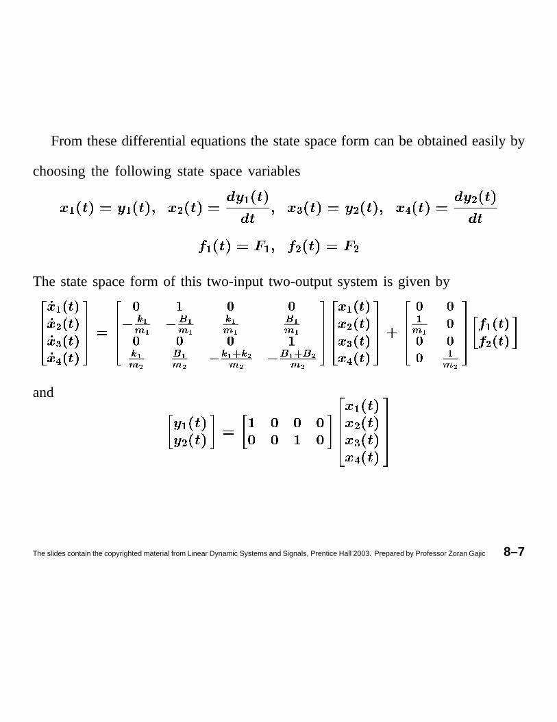
From thesedifferentialequationsthe statespaceform canbe obtainedeasilyby

choosingthe following statespacevariables9 9 : 9 ; : < :9 9 : :

The statespaceform of this two-input two-outputsystemis given by=>>? @A�BDCFEHG@AJIKCFE�G@AML�CFE�G@A3NOCFE�GPRQQS T =>>? U V U UW X�YZ Y W\[JYZ Y X�YZ Y [�YZ YU U U VX�YZ^] [�YZ_] W X�Ya`�X ]Z_] W [JYa`3[ ]Z_]

PRQQS = >>? A�BKCFE�GAJIbC4EHGAMLcC4EHGA3NdC4EHGPRQQSfe =>>? U UBZ Y UU UU BZg]

PRQQSihkj BKC4EHGj I C4EHGmland 9: 9:;<The slides contain the copyrighted material from Linear Dynamic Systems and Signals, Prentice Hall 2003. Prepared by Professor Zoran Gajic 8–7

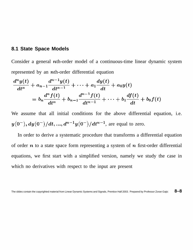
8.1 State Space Models

Considera general th-order model of a continuous-timelinear dynamicsystem

representedby an th-orderdifferential equationn n no*p n�o*pn�o*p p qn n n no*p no*pno*p p qWe assumethat all initial conditions for the above differential equation, i.e.o o no*p o n�o*p

, are equalto zero.

In order to derivea systematicprocedurethat transformsa differentialequation

of order to a statespaceform representinga systemof first-orderdifferential

equations,we first start with a simplified version, namely we study the casein

which no derivativeswith respectto the input are present


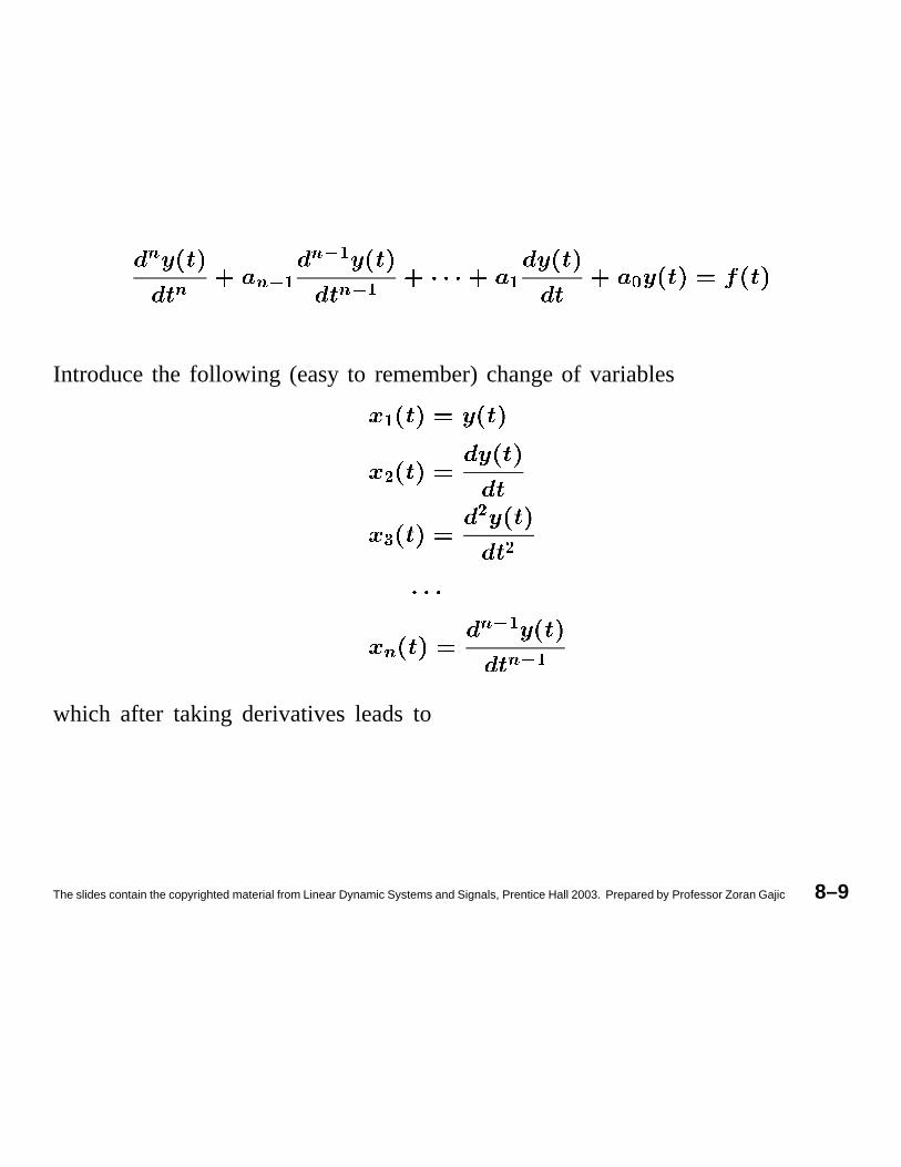
r r r�s*t rs*tr�s*t t uIntroducethe following (easyto remember)changeof variablestvw v v

r r�s*tr�s*twhich after taking derivativesleadsto


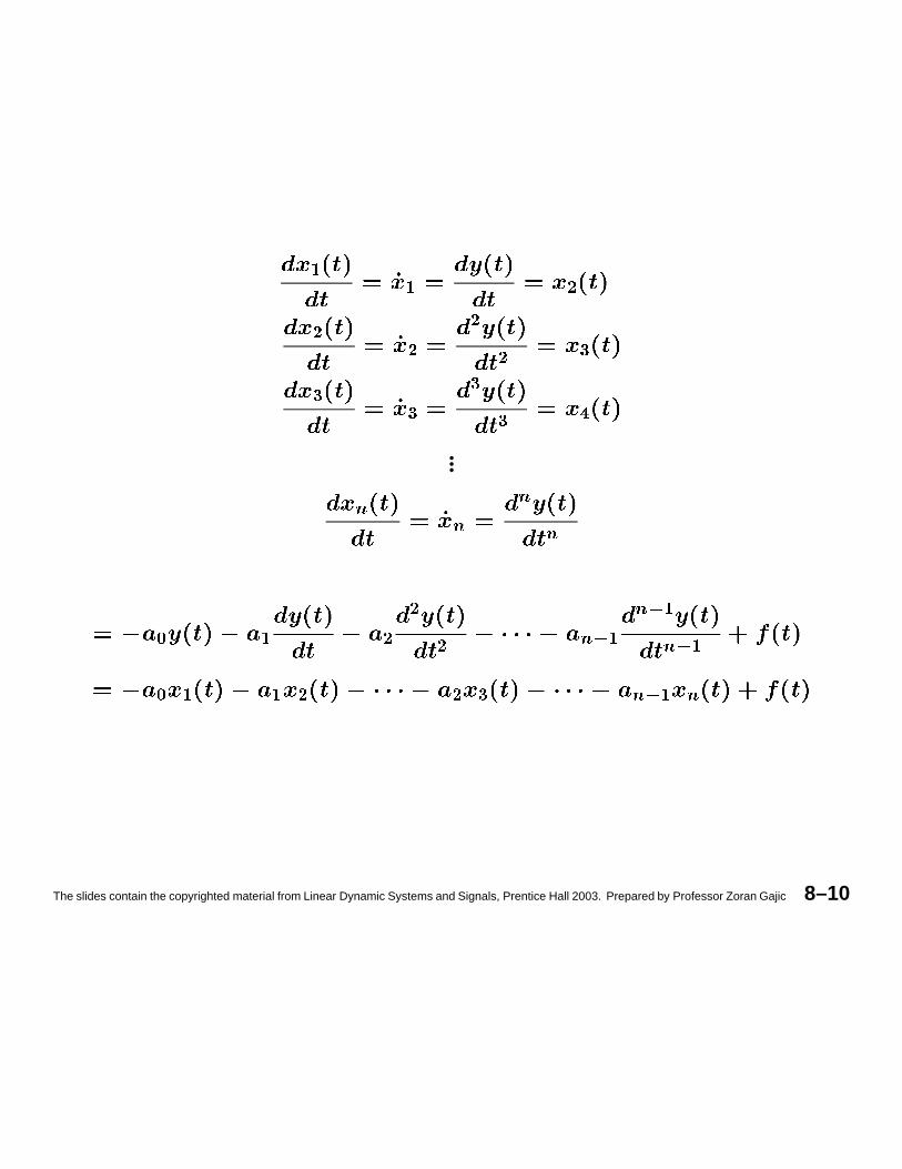
x x yy y y y zz z z z {...| | | |

} x y y y |�~ x |~ x|�~ x} x x y y z |�~ x |


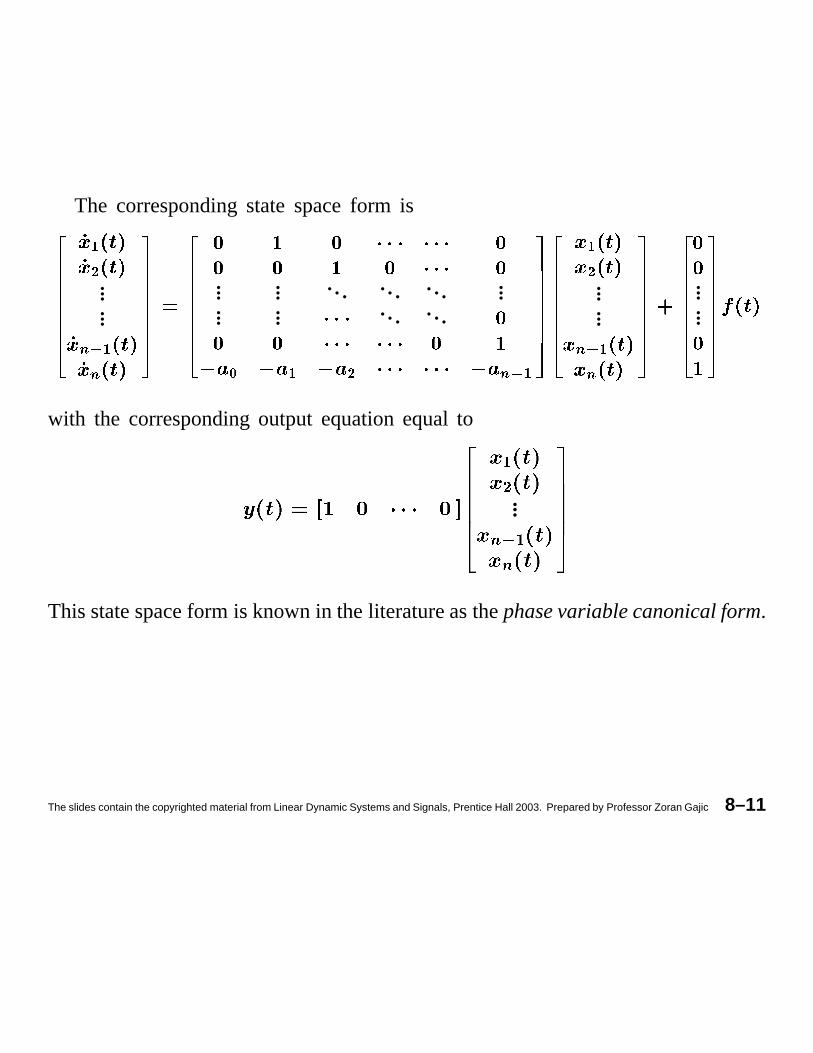
The correspondingstatespaceform is�� D�F�H��J�K�F��......�� 4�H�� 4�H�

�R�� b�b� �b�b� �� b�b� �

... ... . . . . . . . . . ...

... ...�K�b� . . . . . .

�� K�b� �b�b� � �� b�b� �b�b� �� R�� J�b��

...

...�3�� F�� F��R��

�� ......� ��R�� 6��

with the correspondingoutput equationequal to � ...¡�¢ �¡

Thisstatespaceform is knownin theliteratureasthephasevariablecanonicalform.


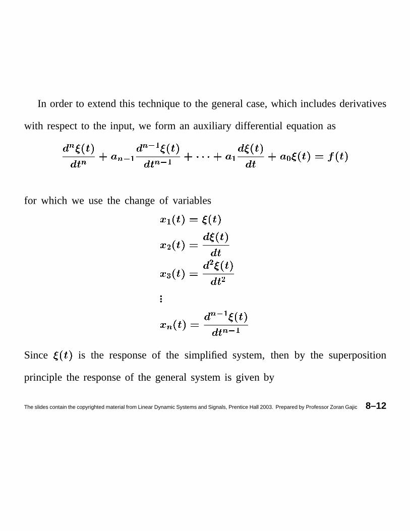
In orderto extendthis techniqueto the generalcase,which includesderivatives

with respectto the input, we form an auxiliary differential equationas£ £ £�¤*¥ £¤*¥£¤*¥ ¥ ¦for which we use the changeof variables¥§¨ § §

... £ £�¤*¥£�¤*¥Since is the responseof the simplified system, then by the superposition

principle the responseof the generalsystemis given by


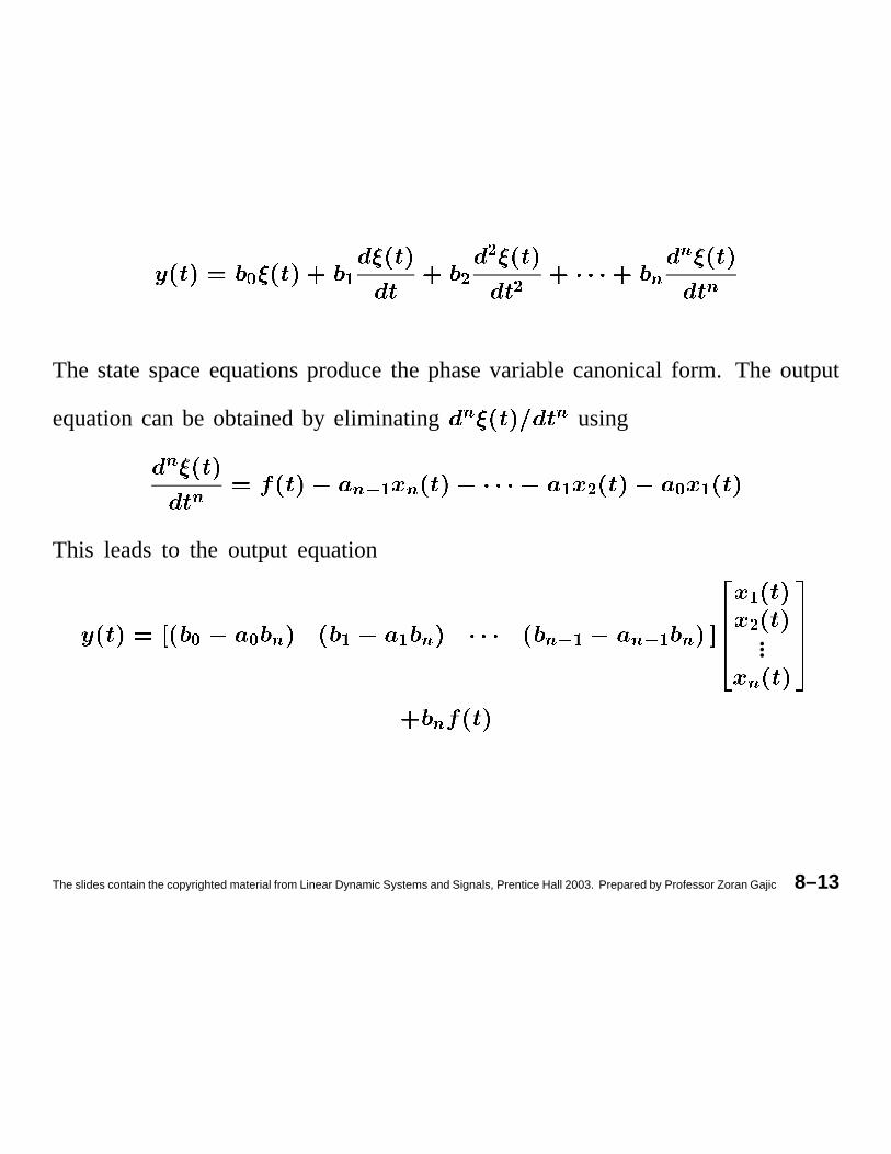
© ª « « « ¬ ¬ ¬The statespaceequationsproducethe phasevariablecanonicalform. The output

equationcan be obtainedby eliminating ¬ ¬ using¬ ¬ ¬� ª ¬ ª « © ªThis leadsto the output equation

© © ¬ ª ª ¬ ¬� ª ¬ ª ¬ ª«...¬¬


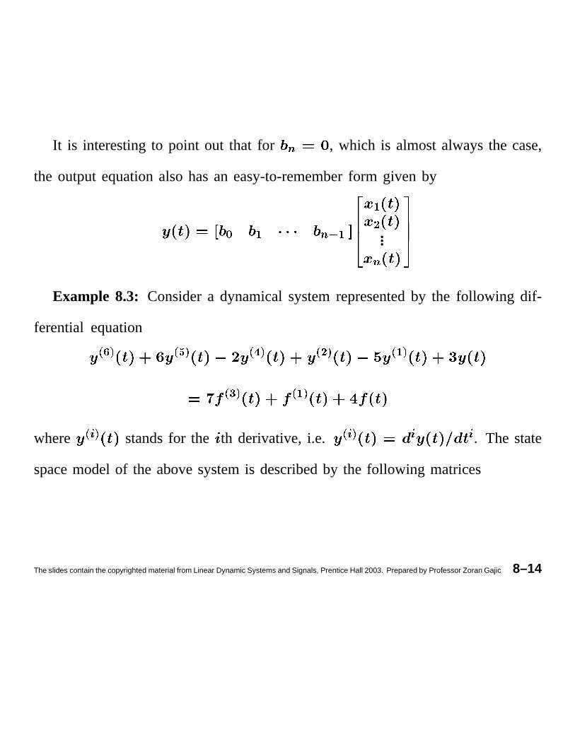
It is interestingto point out that for ® , which is almostalwaysthe case,

the output equationalsohasan easy-to-rememberform given by

¯ ° ®± ° °²...®

Example 8.3: Considera dynamicalsystemrepresentedby the following dif-

ferential equation³µ´H¶ ³¸·�¶ ³º¹�¶ ³ ² ¶ ³ ° ¶³µ»H¶ ³ ° ¶where

³µ¼k¶standsfor the th derivative,i.e.

³µ¼k¶ ¼ ¼. The state

spacemodelof the abovesystemis describedby the following matrices


Note that betweenthe system differential equation and the system transfer

function, definedby ½ ½ ½¾/¿ ½�¾*¿ ¿ À½ ½�¾*¿ ½�¾*¿ ¿ Àthereis the uniquecorrespondence.Hence,the samemethodjust describedcanbe

usedfor obtainingthe statespaceform from the systemtransferfunction.


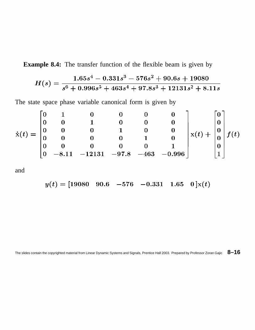
Example 8.4: The transferfunction of the flexible beamis given byÁ Â ÃÄ Å Á Â ÃThe statespacephasevariablecanonicalform is given by

and


8.2 Time Response from the State Equation

The solutionof the statespaceequationscanbeobtainedeitherin the time domain

by solvingthecorrespondingmatrixdifferentialequationdirectlyor in thefrequency

domainby exploiting the power of the Laplacetransform. Both methodswill be

presentedin this section.

8.2.1 Time Domain Solution

For the purposeof solving the stateequation,let us first supposethat the system

is in the scalar form

with a known initial condition Æ . It is very well known from the

elementarytheoryof differentialequationsthat the solution is given by


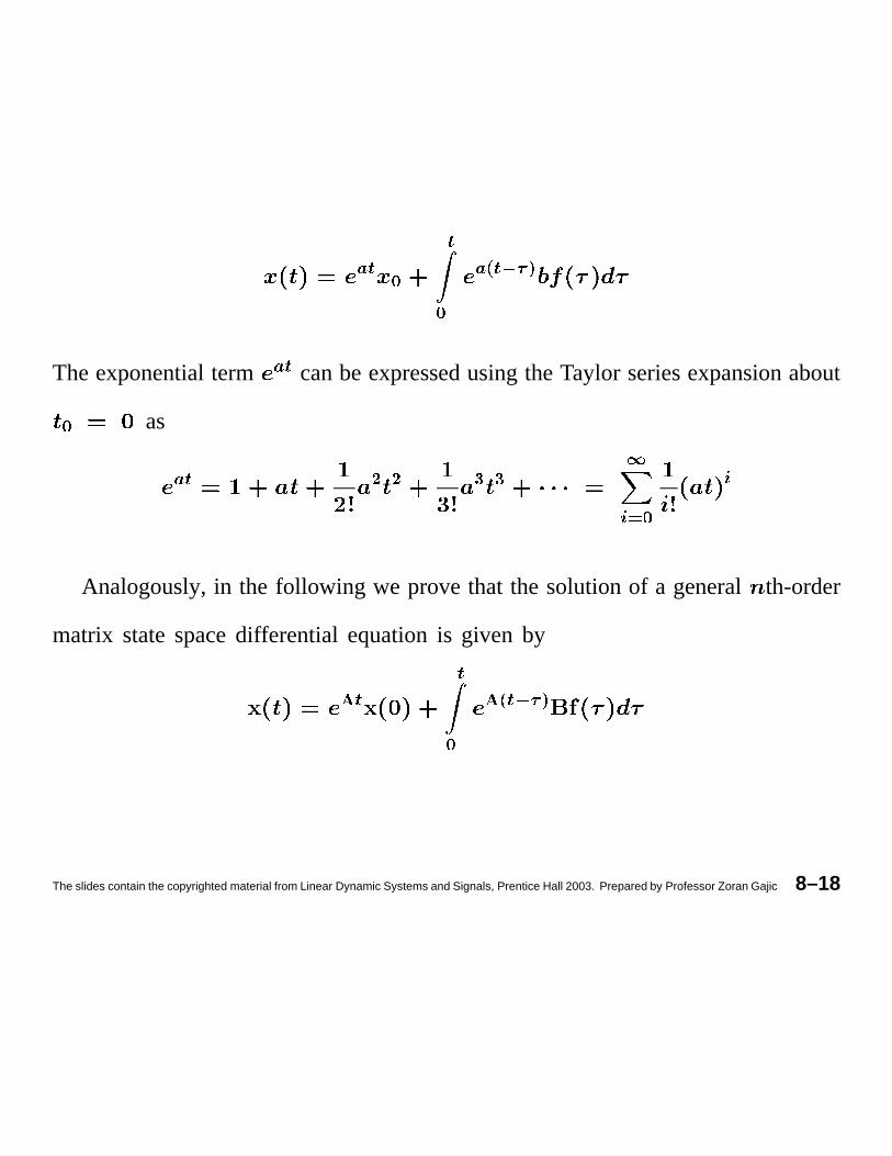
Ç�È É ÈÉ ÇdÊËÈ1ÌÎÍÐÏTheexponentialterm

Ç�ÈcanbeexpressedusingtheTaylor seriesexpansionaboutÉ

as Ç�È Ñ Ñ Ò Ò ÓÔkÕ É ÔAnalogously,in the following we provethat the solutionof a general th-order

matrix statespacedifferential equationis given byÖ È ÈÉ Ö Ê×ÈØÌÍcÏ


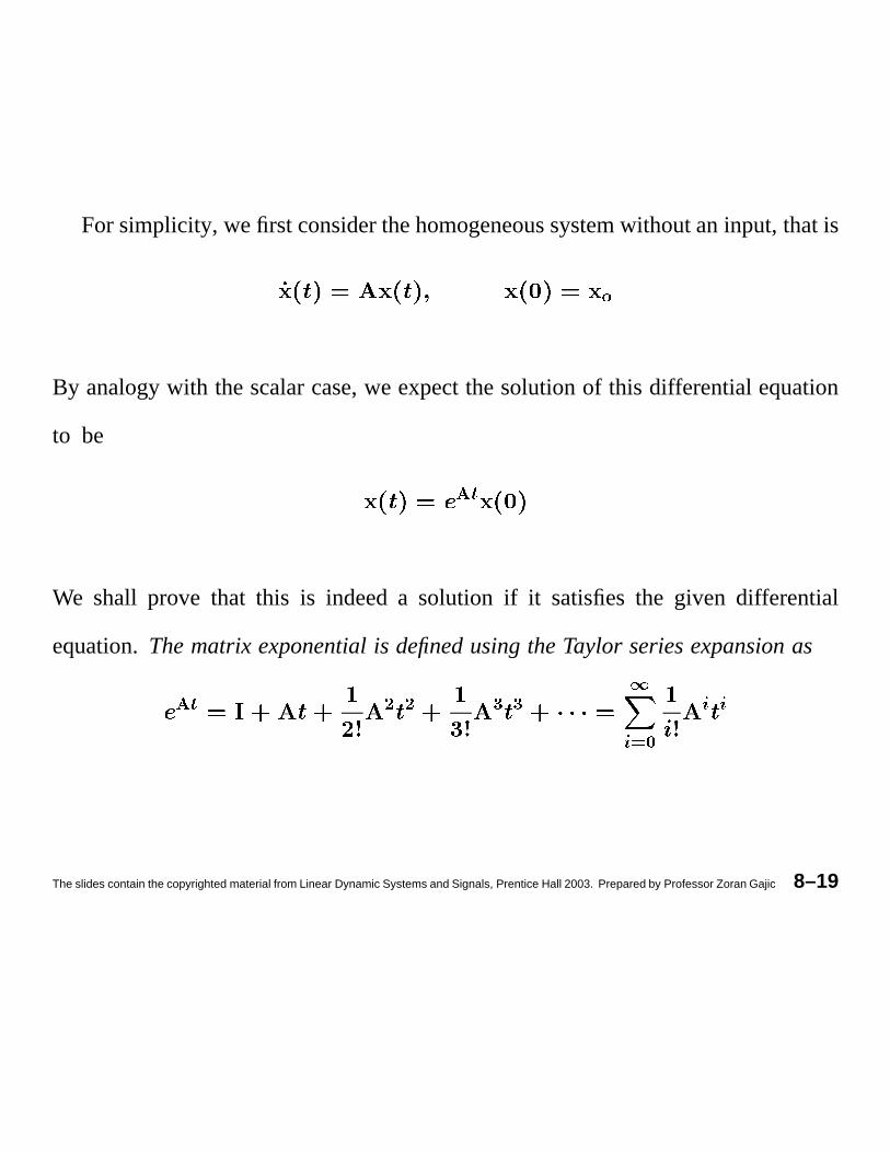
Forsimplicity, wefirst considerthehomogeneoussystemwithoutaninput, thatisÙBy analogywith thescalarcase,we expectthesolutionof this differentialequation

to be Ú�ÛWe shall prove that this is indeeda solution if it satisfiesthe given differential

equation.Thematrix exponentialis definedusingtheTaylor seriesexpansionasÚÎÛ Ü Ü Ý Ý Þßkà.á ß ß


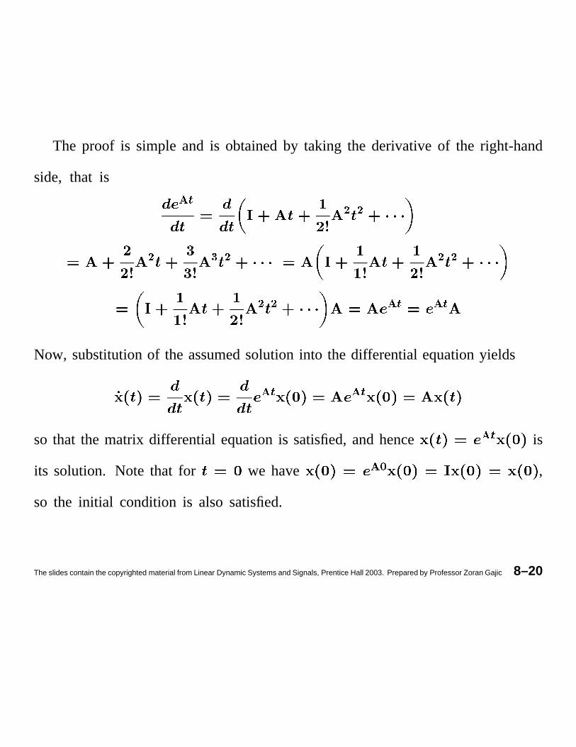
The proof is simple and is obtainedby taking the derivativeof the right-hand

side, that is â�ã ä ää å ä ä ä

ä ä âÎã â�ãNow, substitutionof the assumedsolution into the differentialequationyieldsâ�ã â�ãso that the matrix differential equationis satisfied, andhence

âÎãis

its solution. Note that for we have

â.æ,

so the initial condition is also satisfied.


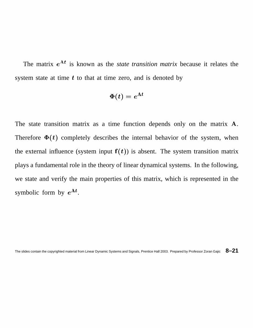
The matrix çÎè is known as the statetransition matrix becauseit relatesthe

systemstateat time to that at time zero, and is denotedbyç�èThe state transition matrix as a time function dependsonly on the matrix .

Therefore completelydescribesthe internal behaviorof the system,when

the externalinfluence(systeminput ) is absent.The systemtransitionmatrix

playsa fundamentalrole in thetheoryof lineardynamicalsystems.In thefollowing,

we stateandverify the main propertiesof this matrix, which is representedin the

symbolic form by ç�è .


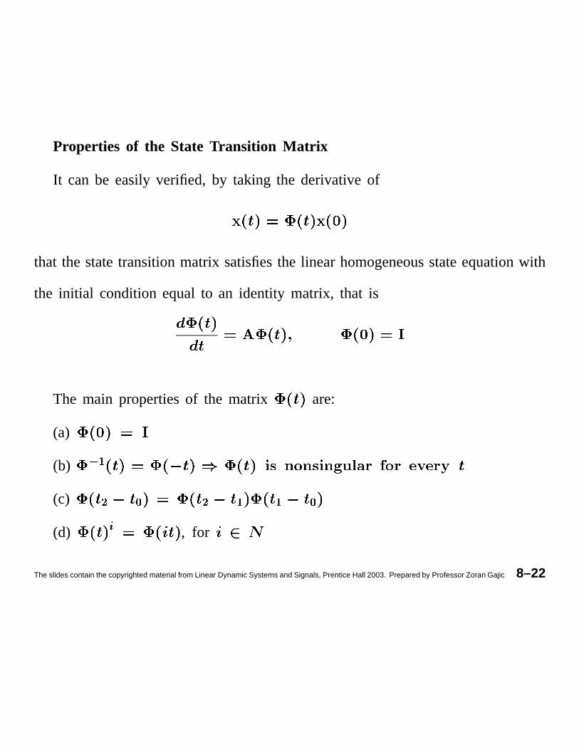
Properties of the State Transition Matrix

It can be easily verified, by taking the derivativeof

that the statetransitionmatrix satisfiesthe linear homogeneousstateequationwith

the initial condition equal to an identity matrix, that is

The main propertiesof the matrix are:

(a)

(b) é*ê(c) ë ì ë ê ê ì(d) í , for


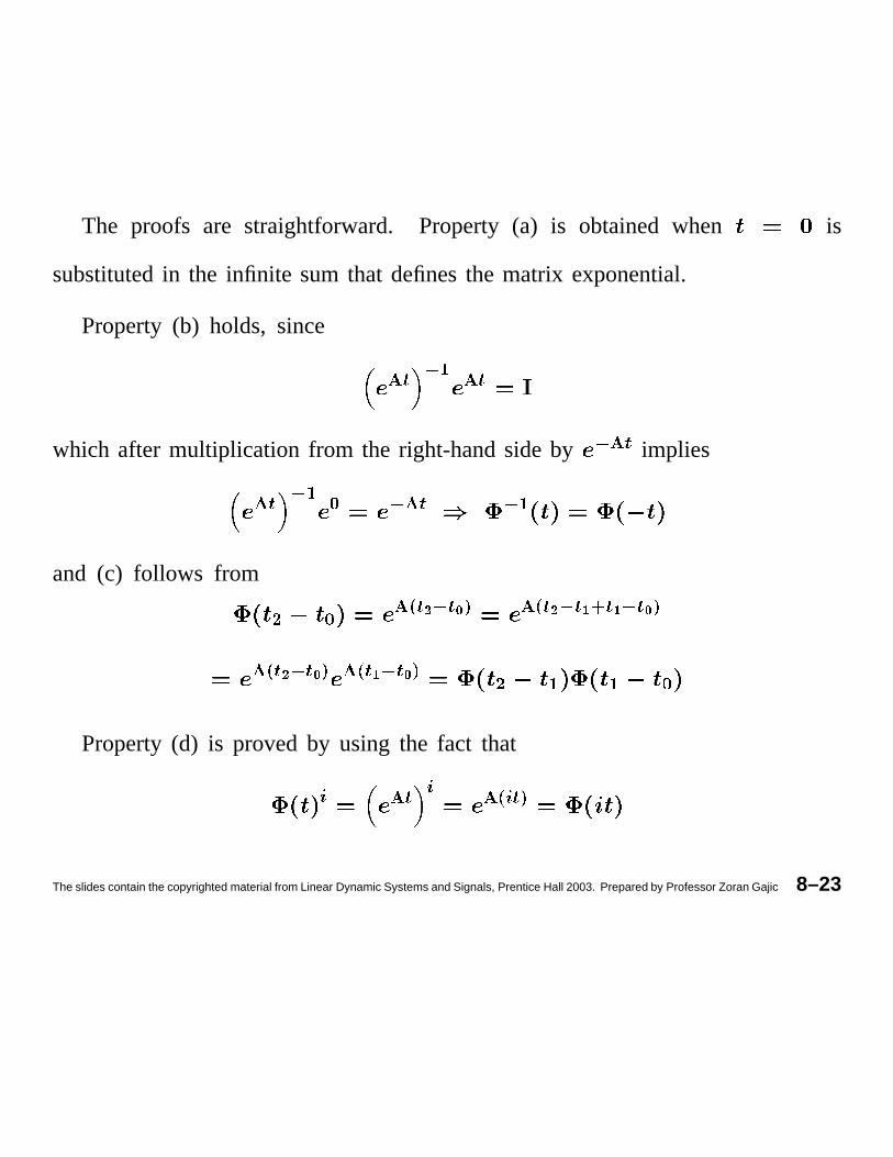
The proofs are straightforward. Property (a) is obtained when is

substitutedin the infinite sum that definesthe matrix exponential.

Property(b) holds, since îï ð.ñ î�ïwhich after multiplication from the right-handsideby

ð î�ïimpliesî�ï ð*ñ ò ð î�ï ð*ñ

and (c) follows from ó ò îõô×ï÷ö ð ï�øúù îûô×ï�ö ð ï4ü,ýï4ü ð ïaø1ùîþô×ï ö ð ï ø ù îûô×ï ü ð ï ø ù ó ñ ñ òProperty(d) is provedby using the fact thatÿ îÎï ÿ îþô ÿ ï ù


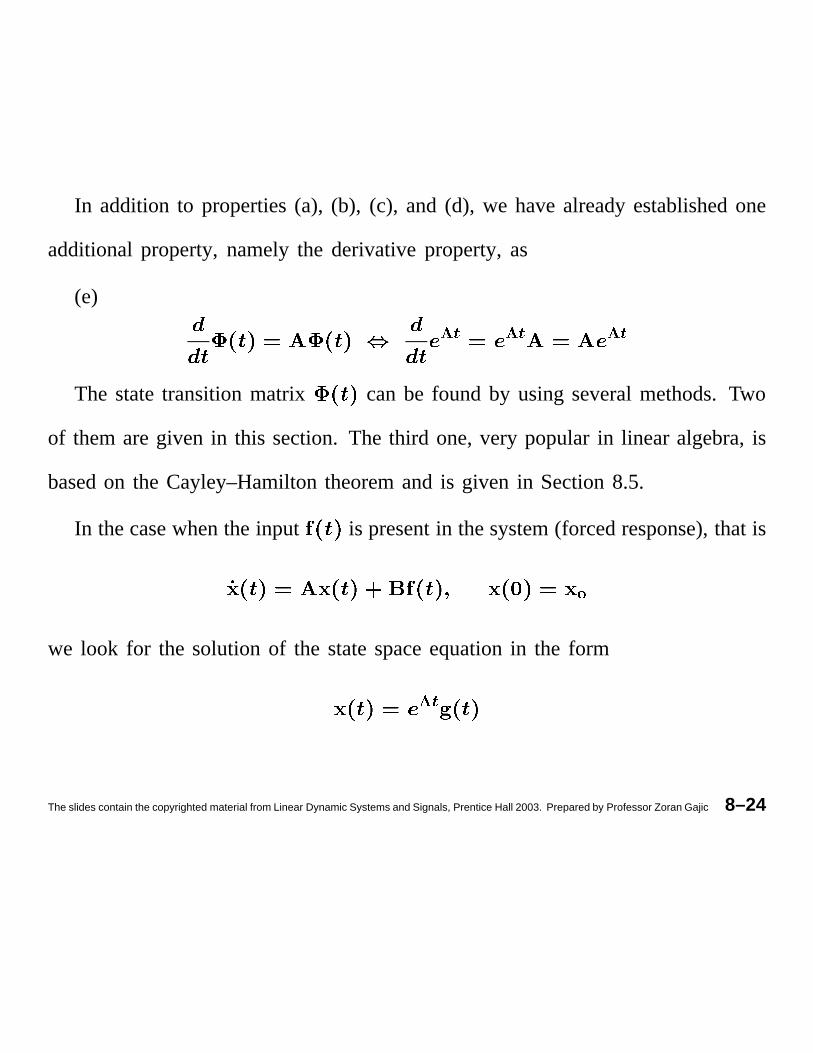
In addition to properties(a), (b), (c), and (d), we havealreadyestablishedone

additionalproperty,namelythe derivativeproperty,as

(e)��

The statetransitionmatrix can be found by usingseveralmethods.Two

of themaregiven in this section.The third one,very popularin linear algebra,is

basedon the Cayley–Hamiltontheoremand is given in Section8.5.

In thecasewhenthe input is presentin thesystem(forcedresponse),that is

�

we look for the solution of the statespaceequationin the form

��


Then��

It follows that

��

and we have

��

Integratingthis equation,bearingin mind that��

, we get

�

��


Substitutionof thelastexpressionin��

givestherequiredsolution

��

��

or �

�

Whenthe initial stateof the systemis known at time � , ratherthanat time ,

the solution of the stateequationis similarly obtainedas

� ��

��

�

� ��


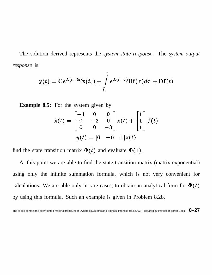
The solution derived representsthe systemstateresponse. The systemoutput

responseis

!�"�#�$�#�%'& (#

# %!�"�#�$�)*&

Example 8.5: For the systemgiven by

find the statetransitionmatrix and evaluate .

At this point we areableto find the statetransitionmatrix (matrix exponential)

using only the infinite summation formula, which is not very convenient for

calculations.We areableonly in rarecases,to obtainan analyticalform for

by using this formula. Suchan exampleis given in Problem8.28.


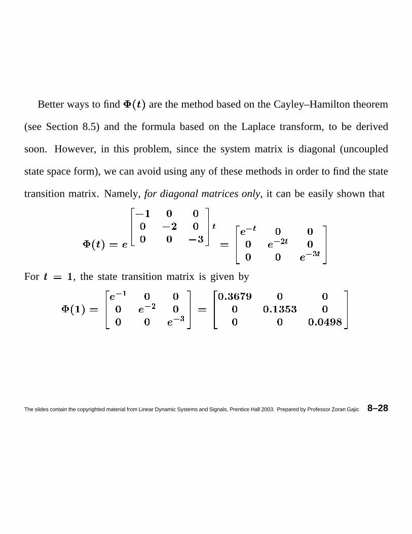
Betterwaysto find arethemethodbasedon theCayley–Hamiltontheorem

(seeSection8.5) and the formula basedon the Laplacetransform,to be derived

soon. However, in this problem,since the systemmatrix is diagonal(uncoupled

statespaceform), we canavoidusinganyof thesemethodsin orderto find thestate

transitionmatrix. Namely,for diagonalmatricesonly, it canbe easilyshownthat

+ , + ,�- + ,�. +For , the statetransitionmatrix is given by,0/

,0-,�.


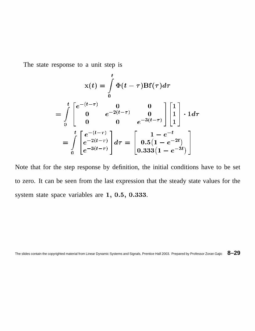
The stateresponseto a unit step is1

21

23�4 1 3�5�6

30784 1 3�5�63�9:4 1 3�5�6

1

23�4 1 3�5�630784 1 3�5�63�9;4 1 3�5�6

3 1307 13�9 1

Note that for the stepresponseby definition, the initial conditionshaveto be set

to zero. It canbe seenfrom the last expressionthat the steadystatevaluesfor the

systemstatespacevariablesare .


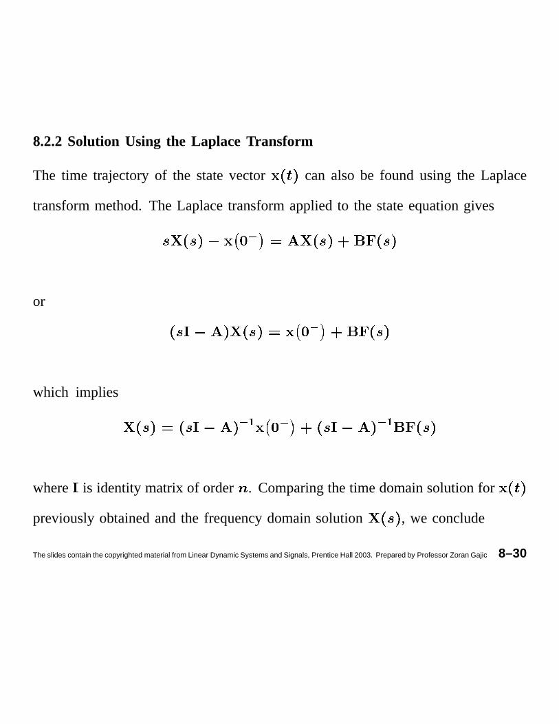
8.2.2 Solution Using the Laplace Transform

The time trajectoryof the statevector can also be found using the Laplace

transformmethod.The Laplacetransformappliedto the stateequationgives

<

or

<

which implies

<�= < <�=

where is identity matrix of order . Comparingthetime domainsolutionfor

previouslyobtainedandthe frequencydomainsolution , we conclude


>@?

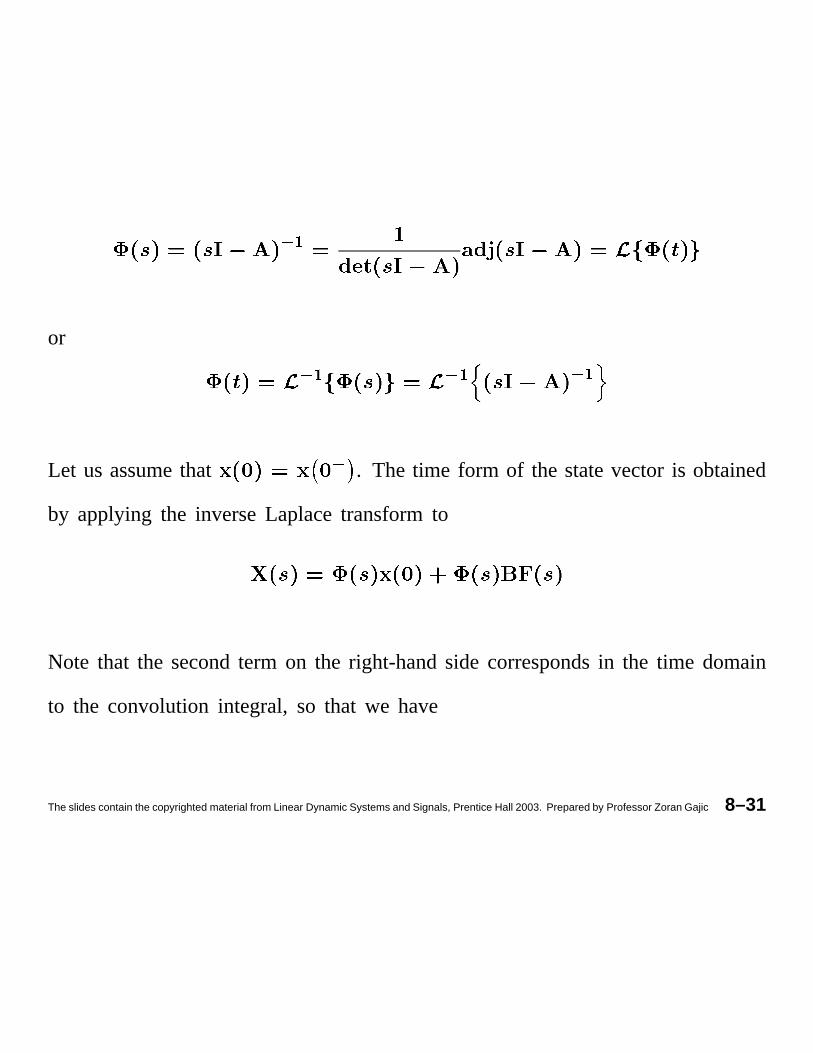
or

>�? >�? >�?

Let us assumethat>

. The time form of the statevector is obtained

by applying the inverseLaplacetransformto

Note that the secondterm on the right-handside correspondsin the time domain

to the convolution integral, so that we have


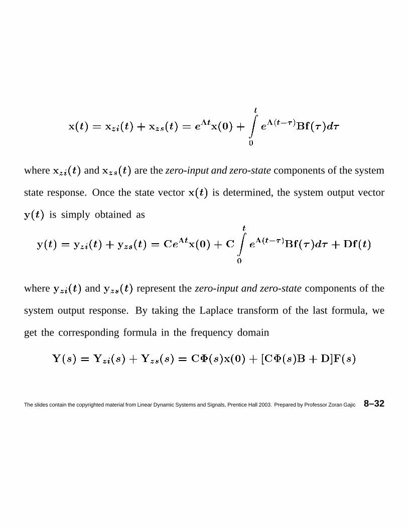
A8B A;C D�EE

FD�G�E�H�I�J

where A8B and A;C arethezero-inputandzero-statecomponentsof thesystem

stateresponse.Oncethe statevector is determined,the systemoutputvector

is simply obtainedas

A8B A;C D�EE

FD�G�E�H�I�J

where A8B and A;C representthezero-inputandzero-statecomponentsof the

systemoutput response.By taking the Laplacetransformof the last formula, we

get the correspondingformula in the frequencydomain

A8B A;C


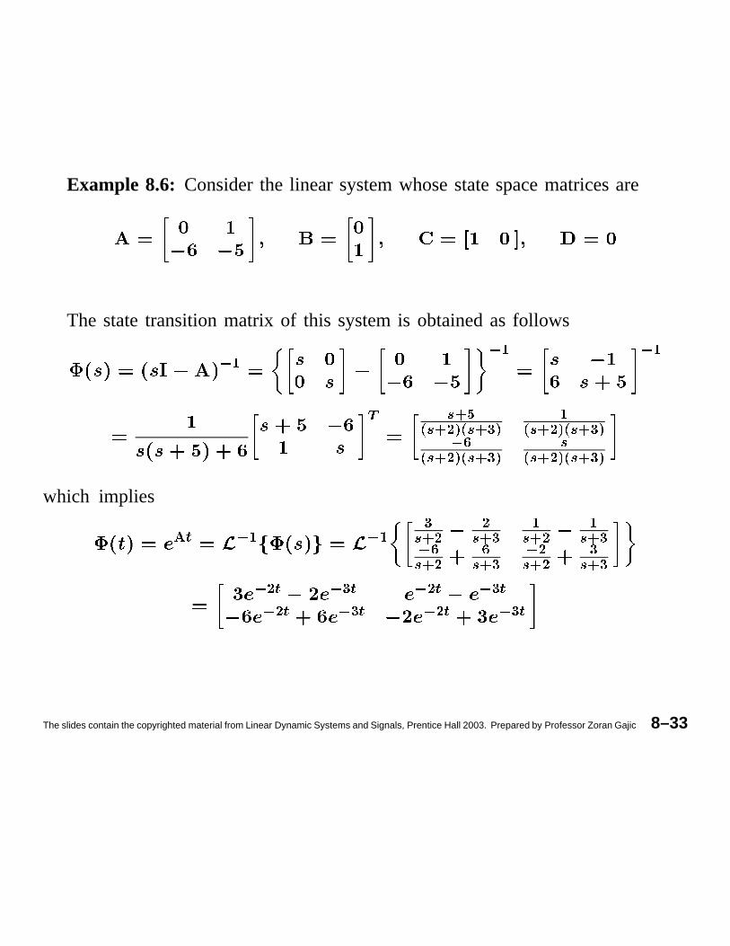
Example 8.6: Considerthe linear systemwhosestatespacematricesare

The statetransitionmatrix of this systemis obtainedas follows

K0L K�L K�L

M NPO@QR NSO�TVU R NWO�XYU LR NSO�TVU R NWO�XYUK�ZR NSO�TVU R NWO�XYU NR NSO�TVU R NWO�XYUwhich implies

[�\ K�L K�L XNWO]T TNSO@X LNSO�T LNWO�XK�ZNWO]T ZNSO@X K TNSO�T XNWO�XK T \ K X \ K T \ K X \K T \ K X \ K T \ K X \


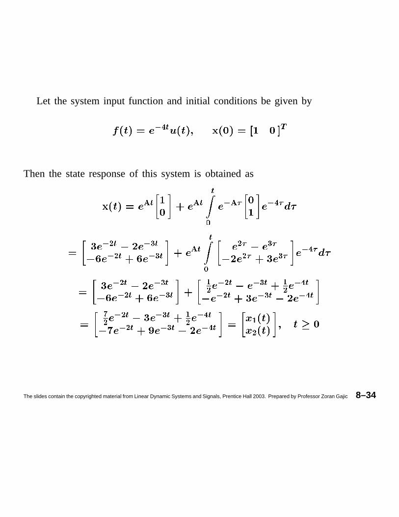
Let the systeminput function and initial conditionsbe given by

^�_a` b

Then the stateresponseof this systemis obtainedas

c ` c ``

d^ c�e ^�_ e

^�fS` ^�gP`^0fS` ^�gP` c `

`d

f e g ef e g e ^�_ e

^0fS` ^�gP`^0fS` ^�gP`

hf ^0fS` ^�gP` hf ^�_P`^0fS` ^�gP` ^�_P`

if ^0fS` ^�gP` hf ^�_P`^0fS` ^�gP` ^�_P` h

f


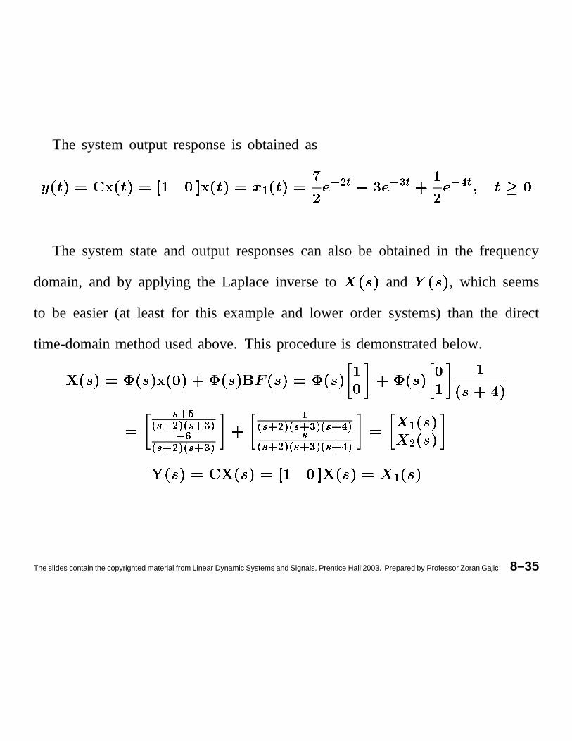
The systemoutput responseis obtainedas

j k�lSm k�nPm k�oPm

The systemstateand output responsescan also be obtainedin the frequency

domain, and by applying the Laplaceinverseto and , which seems

to be easier(at least for this exampleand lower order systems)than the direct

time-domainmethodusedabove.This procedureis demonstratedbelow.

pPq@rs pSq lVt s pSq nutk�vs pSq lVt s pSq nutjs pSq lVt s pWq nwt s pSq outps pSq lVt s pWq nwt s pSq out

jl

j


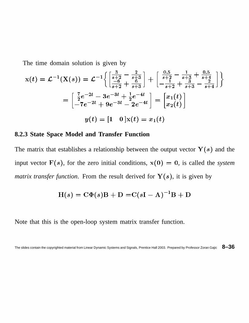
The time domainsolution is given by

x@y x�y z{}|0~ ~{W| zx��{S|�~ �{W| z�:��{S|�~ y{W| z �8��{S|@�y{S|�~ z{W| z ~{S|@��~ x ~S� x z � y~ x �P�

x ~S� x z � x �P� y~y

8.2.3 State Space Model and Transfer Function

The matrix that establishesa relationshipbetweenthe outputvector and the

input vector , for the zero initial conditions, , is called the system

matrix transferfunction. From the resultderivedfor , it is given by

x�y

Note that this is the open-loopsystemmatrix transferfunction.


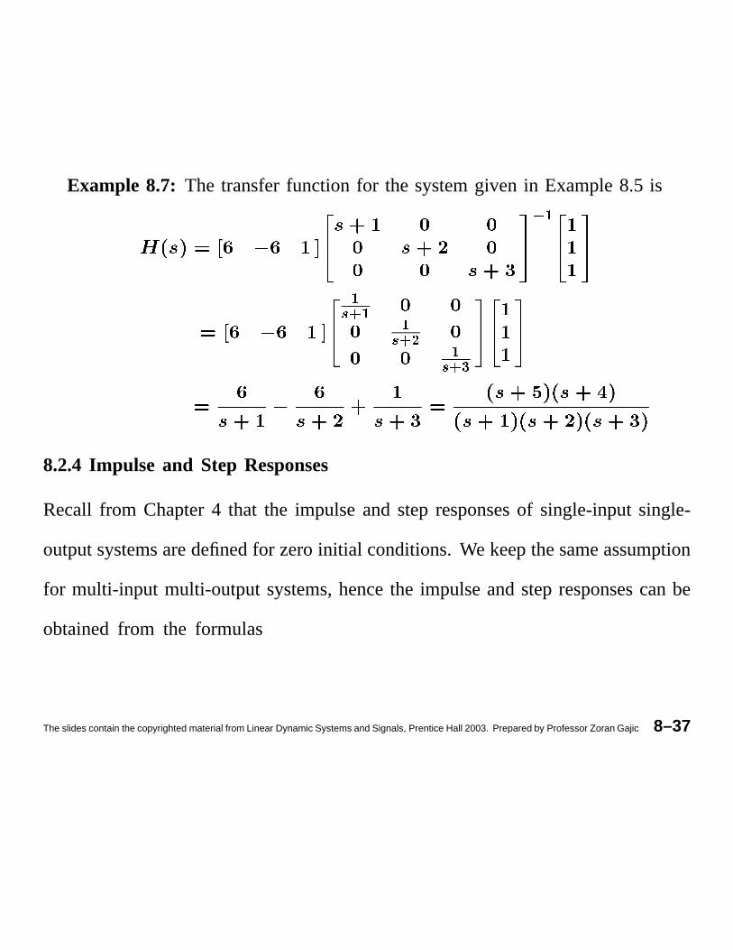
Example 8.7: The transferfunction for the systemgiven in Example8.5 is�0�

��P� � ��W�]� ��S�@�

8.2.4 Impulse and Step Responses

Recall from Chapter4 that the impulseand stepresponsesof single-inputsingle-

outputsystemsaredefinedfor zeroinitial conditions.We keepthesameassumption

for multi-input multi-outputsystems,hencethe impulseandstepresponsescanbe

obtainedfrom the formulas


�

�� *�

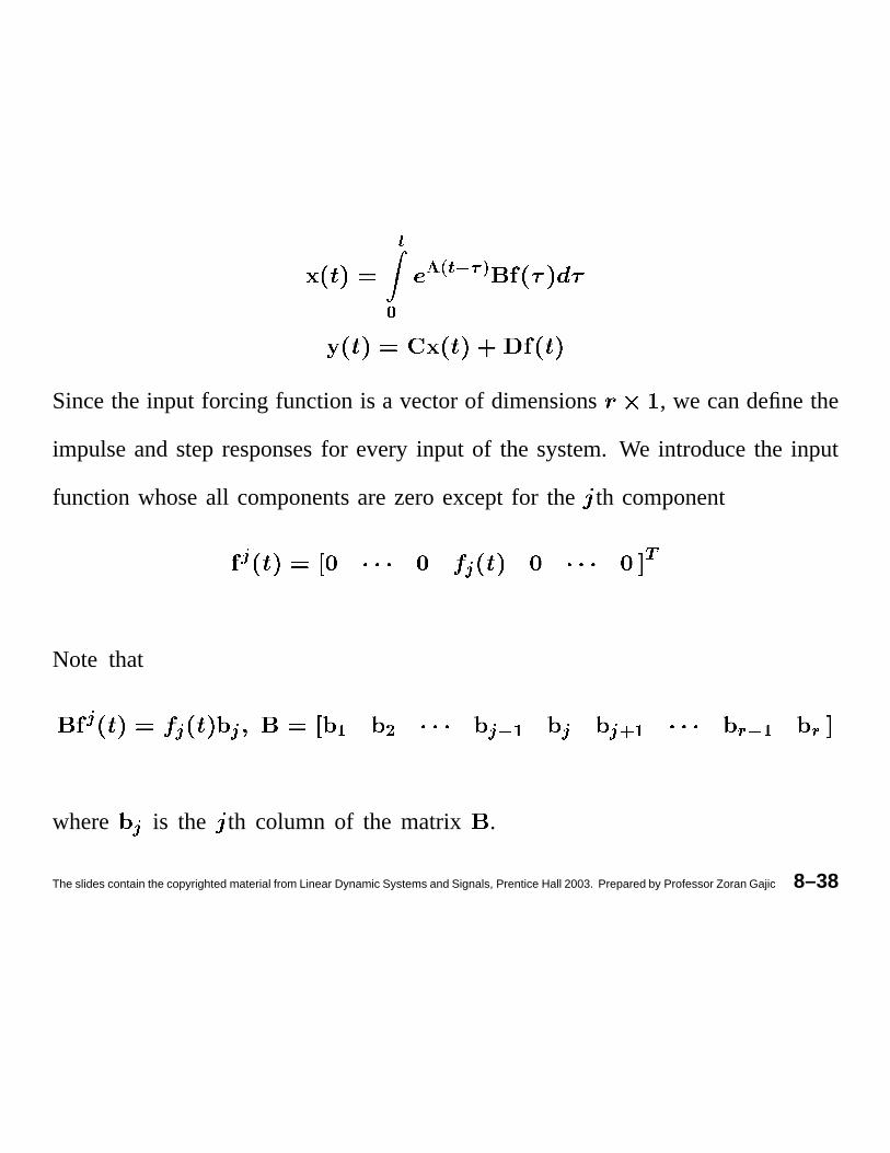
Sincethe input forcing function is a vectorof dimensions , we candefinethe

impulseandstepresponsesfor every input of the system.We introducethe input

function whoseall componentsarezeroexceptfor the th component

� � �

Note that

� � � � � � � � � ��

where � is the th column of the matrix .


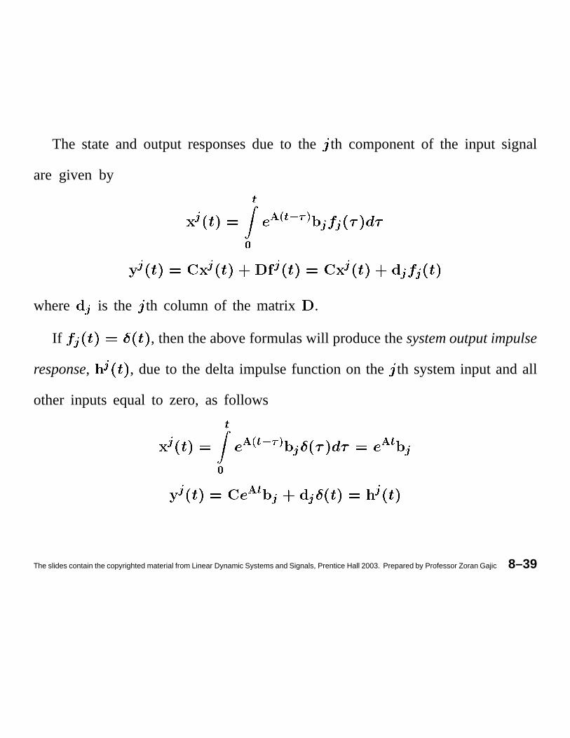
The stateand output responsesdue to the th componentof the input signal

are given by

� �

¡�¢ �¤£�¥§¦ � �

� � � � � �where � is the th column of the matrix .

If � , thentheaboveformulaswill producethesystemoutputimpulse

response,�

, due to the delta impulsefunction on the th systeminput andall

other inputs equal to zero, as follows

� �

¡�¢ �¤£�¥¨¦ � ¡ � �

� ¡ � � � �


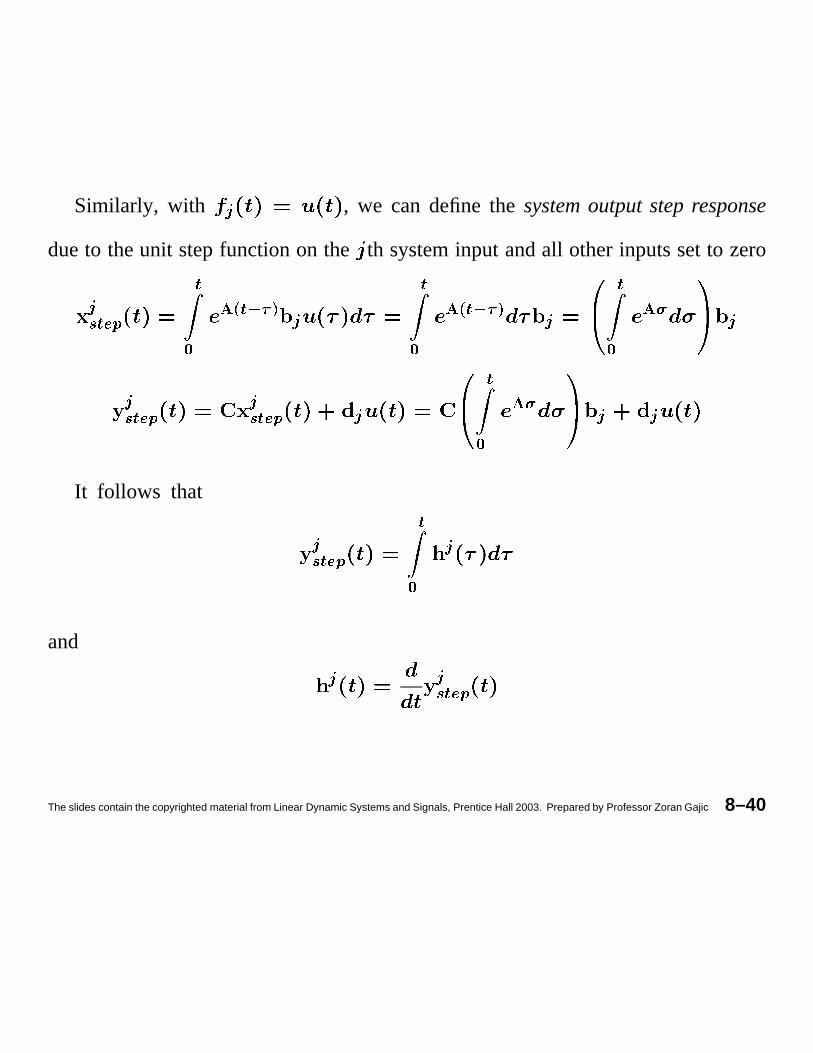
Similarly, with © , we can definethe systemoutputstepresponse

dueto theunit stepfunctionon the th systeminput andall otherinputssetto zero

© ª¤«¬®«

¯°�± «�²�³*´

©«

¯°�± «¤²�³�´

©«

¯°¶µ ©

© ª·«¬�® © ª�«¸¬�® ©«

¯°¶µ © ©

It follows that

© ª·«¬�®«

¯©

and

© © ª�«¸¬�®


Documents

Continuous-Time State Space Analysis