Continuum damage growth analysis using …apm.iitm.ac.in/smlab/mss/download/52.pdfContinuum damage growth analysis using element free Galerkin method 281 Figure 1. Mechanical representation

Sadhana Vol. 35, Part 3, June 2010, pp. 279–301. © Indian Academy of Sciences

Continuum damage growth analysis using element freeGalerkin method

C O ARUN, B N RAO∗ and S M SRINIVASAN

Structural Engineering Division, Department of Civil Engineering, IndianInstitute of Technology Madras, Chennai 600 036e-mail: [email protected]

MS received 30 December 2008; revised 14 August 2009; accepted 15 December2009

Abstract. This paper presents an elasto-plastic element free Galerkin formula-tion based on Newton–Raphson algorithm for damage growth analysis. Isotropicductile damage evolution law is used. A study has been carried out in this paperusing the proposed element free Galerkin method to understand the effect of initialdamage and its growth on structural response of single and bi-material problems.A simple method is adopted for enforcing EBCs by scaling the function approxima-tion using a scaling matrix, when non-singular weight functions are used over theentire domain of the problem definition. Numerical examples comprising of one-and two-dimensional problems are presented to illustrate the effectiveness of theproposed method in analysis of uniform and non-uniform damage evolution prob-lems. Effect of material discontinuity on damage growth analysis is also presented.

Keywords. Damage mechanics; mesh-free method; elasto-plastic element freeGalerkin method; essential boundary condition; material discontinuity.

1. Introduction

Damage is a progressive physical mechanism which leads to the initiation and growth ofmicro-voids or micro-cracks. Proper understanding of damage growth is essential to under-stand the effect of the presence of voids and internal defects on the global response ofmechanical/structural system and also on the process which leads these internal defects tofinal fracture. Evolutionary concept of damage mechanics is proposed by Kachanov (1958),which is based on one-dimensional surface damage variable. Later, an effective stress con-cept (Rabotnov 1969) associated with strain equivalence principle (Lemaitre 1971) is devel-oped. A well-documented research on damage mechanics is available elsewhere (Lemaitre1985; Chaboche 1988; Chaboche 1988; Voyiadjis & Kattan 1990; Lemaitre 1992; Lemaitre &Desmorat 2005; Voyiadjis & Kattan 2005). For implementation of damage coupled nonlin-ear equations in finite element method (FEM), Benallal et al (1988) proposed an integration

∗For correspondence

279

280 C O Arun, B N Rao and S M Srinivasan

algorithm based on Newton method, to solve the nonlinear global equilibrium equations aswell as the nonlinear local equations obtained by fully implicit integration of the constitutiveequations. The applications of different damage models and analysis using numerical toolslike FEM are well-explained by Kattan & Voyiadjis (2002). In recent years mesh-free meth-ods are becoming increasingly popular in the areas of fracture mechanics and related topics.

Mesh-free methods such as smooth particle hydrodynamics (Lucy 1977; Monaghan 1988)diffuse element method (Nayroles et al 1992), element free Galerkin method (EFGM)(Belytschko et al 1994; Lu et al 1994; Belytschko et al 1995), h–p clouds (Duarte & Oden1996), partition of unity (Melenk & Babuska 1996), and reproducing kernel particle method(RKPM) (Liu et al 1995; Liu et al 1997) have been demonstrated particularly attractive forvarious reasons as they avoid burdensome mesh generation, can easily model the evolutionof discontinuities such as cracks and interfaces. Among these methods, EFGM is particularlyappealing, due to its simplicity, alleviation of numerical difficulties of mesh entanglement,faster rate of convergence, and formulation that corresponds to well-established FEM. Themain drawback that EFGM faced is the problems associated with imposition of the essentialboundary conditions (EBCs). Use of non-singular weight functions for moving least square(MLS) approximation will lead to lack of Kronecker delta property of EFGM shape functions,and further leads to difficulties in imposition of EBCs. Researchers came up with differentmethods to address this problem, like coupled finite element-EFGM (Krongauz & Belytschko1996), Lagrange multiplier technique (Dolbow & Belytschko 1998), penalty method (Liu2002), full transformation method (Chen & Wang 2000; Arun et al 2007), extended partitionof unity finite element (PUFEM) weight function (Alves & Rossi 2003), etc. Efficiency ofEFGM has been demonstrated in the areas of crack propagation (Rao & Rahman, 2000; Luet al 1995), moving boundaries (Li & Belytschko 2001), large deformation problems (Pon-thot & Belytschko 1998), and others (Nagashima 1999). However, damage analysis usingmesh-free techniques has not received much attention. Alves & Rossi (2003) presented amethod which combines the element-free Galerkin with an extended PUFEM, that is ableto enforce, in some limiting sense, the essential boundary conditions as done in the FEMand solved some coupled elasto-plastic damage problems using the integration algorithmproposed by Benalall et al (1988). This method requires an iterative scheme for solvingglobal equilibrium equations and also for the local integration of constitutive equations. Thiswill enhance the computational cost required. Moreover, combining extended PUFEM withEFGM can increase the computational complexity of the problem.

In this paper, elasto-plastic element free Galerkin formulation is presented based onNewton–Raphson method for solving the global equilibrium equations and a simple implicitalgorithm (Sivakumar & Voyiadjis 1997) for local integration of constitutive equations. Theeffect of initial damage on further material behaviour is analysed, since always there existsa probability that an initial damage in the form of micro-cracks or micro-voids be present inall engineering materials and hence materials behave differently from what is expected. Thepresence of damage in problems with material discontinuities, such as bimaterial problems,is also considered in the present work as different material properties will lead to differentrate of damage growth in each of the materials and will affect the interface stresses andstrains. In the present work a method using transformation matrix, by which the displace-ment approximations are scaled along the essential boundaries to get the Kronecker deltaproperties (Arun et al 2009), is used for EBC and material discontinuity treatment. Isotropicdamage evolution law (Lemaitre 1985; Lemaitre & Desmorat 2005) is used in this study. Thepaper is organized as follows. Section 2 presents a brief outline of continuum damage theory.Section 3 describes elasto-plastic EFGM formulation for damage mechanics, imposition of

Continuum damage growth analysis using element free Galerkin method 281

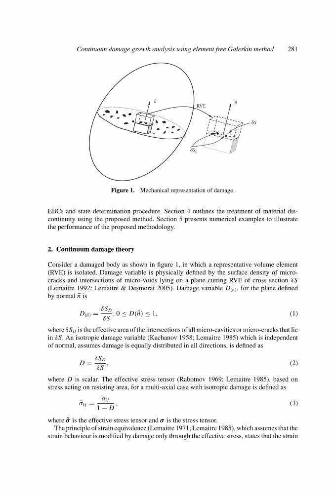
Figure 1. Mechanical representation of damage.

EBCs and state determination procedure. Section 4 outlines the treatment of material dis-continuity using the proposed method. Section 5 presents numerical examples to illustratethe performance of the proposed methodology.

2. Continuum damage theory

Consider a damaged body as shown in figure 1, in which a representative volume element(RVE) is isolated. Damage variable is physically defined by the surface density of micro-cracks and intersections of micro-voids lying on a plane cutting RVE of cross section δS

(Lemaitre 1992; Lemaitre & Desmorat 2005). Damage variable D(�n), for the plane definedby normal �n is

D(�n) = δSD

δS, 0 ≤ D(�n) ≤ 1, (1)

where δSD is the effective area of the intersections of all micro-cavities or micro-cracks that liein δS. An isotropic damage variable (Kachanov 1958; Lemaitre 1985) which is independentof normal, assumes damage is equally distributed in all directions, is defined as

D = δSD

δS, (2)

where D is scalar. The effective stress tensor (Rabotnov 1969; Lemaitre 1985), based onstress acting on resisting area, for a multi-axial case with isotropic damage is defined as

σij = σij

1 − D, (3)

where σσσ is the effective stress tensor and σσσ is the stress tensor.The principle of strain equivalence (Lemaitre 1971; Lemaitre 1985), which assumes that the

strain behaviour is modified by damage only through the effective stress, states that the strain


constitutive equations for a damaged material can be derived using the same formulationsused for an undamaged material except that the stress is replaced by the effective stress. Thethermodynamics of damage along with elasticity and plasticity is included in the isotropicunified damage law (Lemaitre 1992; Lemaitre & Desmorat 2005), which is briefly discussedbelow.

According to isotropic unified damage law, the main variable governing the damage evo-lution is the damage rate and the associated variable is the energy density release rate(Lemaitre & Desmorat 2005). The dissipative potential function, F is defined as

F = f + Fχ + FD, (4)

where f is the plasticity criterion function defined as,

f = (σσσ − χχχ)eq − κ − σY , (5)

where κ is the isotropic hardening stress variable, χχχ is the back stress related to kinematichardening, σY is the yield stress and

(σσσ − χχχ)eq =√

3

2(σD

ij − χDij )(σD

ij − χDij ). (6)

Fχ is the nonlinear kinematic hardening term modelled by

Fχ = 3γ

4cχijχij , (7)

with c and γ are the temperature dependent material parameters. For linear kineamatic hard-ening γ is set to zero. FD is the damage potential defined as

FD = S

(s + 1)(1 − D)

(Y

S

)s+1

, (8)

where S and s are the material parameters which depends on temperature, and Y is the energydensity rate given by

Y = σ 2eqRv

2E0, (9)

where Rv is the triaxiality function defined by

Rv = 2

3(1 + ν) + 3(1 − 2ν)

(σH

σeq

)2

, (10)

where ν is the poison ratio, σH = σkk/3 is the hydrostatic stress, σeq =√

32σD

ij σDij is the von

Mises equivalent stress with the stress deviator, σDij = σij − σHδij , and σeq = σeq(1 − D) is

the effective von Mises stress. E0 is the Young’s modulus of virgin material.


The evolution laws of internal variables are derived as

εp

ij = λ∂F

∂σij

= λ∂f

∂σij

, (11)

αij = −λ∂F

∂χij

, (12)

v = −λ∂F

∂κ, (13)

and

D = λ∂F

∂Y= λ

∂FD

∂Y, (14)

where λ is the plastic multiplier obtained by the consistency conditions, f = 0 and f = 0.εεεp is plastic strain tensor, ααα is kinematic hardening state variable, and υ is isotropic hardeningstate variable.

Using equations (8) and (14) the damage constitutive equation is derived as

D ={(

YS

)s λ(1−D)

, if p > pD

0, if not

D = Dc → meso-crack initiation, (15)

where D is the damage rate, p is the accumulated plastic strain defined by p =√

23ε

p

ij εp

ij for

von Mises yield criteria, and Dc is the critical damage value at which the meso-crack initiationsoccur, which is a material parameter. The damage threshold, pD which is the accumulatedplastic strain at which damage starts, is defined as

pD = εpD for monotonic loading

pD = εpD

(σu − σ∞

f

σeq max+σeq min

2 − σ∞f

)m

for cyclic loading, (16)

where εpD is the damage threshold in pure tension, m is the correction parameter, σu is theultimate stress and σ∞

f is the asymptotic fatigue stress.In the present study an initial damage is assumed to present in the material and so a realistic

assumption that damage will start to grow once the hardening starts is considered. Howeverdamage closure effect is not considered in this study.

3. Elasto-plastic EFGM formulation for damage mechanics

3.1 Variational formulation and discretization

For small displacements in two-dimensional problems with isotropic damage, the equilibriumequations and boundary conditions can be written in terms of effective stress as

∇∇∇ · ((111 − D)σσσ ) + bbb = 0 in �, (17)

((111 − D)σσσ ) · nnn = ttt on t (natural boundary conditions), (18)

uuu = uuu on u (essential boundary conditions), (19)


where, σσσ is the effective stress vector, bbb is the body force vector, ttt and uuu are the vectors ofprescribed surface tractions and displacements, respectively, nnn is a unit normal to domain�, t and u are the portions of boundary, where tractions and displacements are prescribed,respectively, and ∇∇∇T === {∂/∂x1, ∂/∂x2} is the vector of gradient operators. The variationalform of the equation (17) can be written as∫

�

(1 − D)δεεεT σσσd� −∫

�

δuuuTbbbd� −∫

f

δuuuT tttd = 0, (20)

where δuuu and δεεε are virtual displacement increment and strain increment respectively. Usingmeshless discretization of the domain, the MLS (Lancaster & Salkauskas 1981) approximationof displacement vector uuu, is given by (Belytschko et al 1994; Rao & Rahman 2000)

uh(x) =n∑

I=1

�I(xxx)dI = ��T (xxx)ddd, (21)

where n is the number of nodes influencing xxx, ��T (xxx) = {�1(xxx), �2(xxx), . . . , �n(xxx)}, with�I(xxx) representing the shape function of MLS approximation corresponding to node I , anddddT = {d1, d2, . . . , dn} with dI representing the nodal parameter (not the nodal values ofuh(xxx)) for node I . Substituting of equation (21) into equation (20) results in∫

�

(1 − D)BBBT σσσd� = RRR, (22)

where BBB is the strain displacement matrix. For node I , BBB is given by

BBBI =�I,1 0

0 �I,2

�I,2 �I,1

, (23)

and RRR is the external equivalent force vector, defined by

RRRI =∫

�

�Ibbbd� −∫

f

�I tttd ∈ �2. (24)

For analysis which includes material nonlinearity, equation (22) becomes a nonlinear functionof the displacement and so a nonlinear function of the nodal parameter vector, ddd . Henceiterative methods are needed for solving the equation (22). Since an elasto-plastic constitutiverelation depends on deformation history, an incremental analysis following an actual variationof external forces should be used to trace the variation of displacement, strain, and stressalong with external forces. Newton–Raphson method (Chen & Han 1988), is used to solvethe global equilibrium equations where as a simple implicit scheme (Sivakumar & Voyiadjis1997) is used to solve the constrained elasto-plastic damage evolution equations and forupdating variables.

The load RRR, is applied incrementally to the mechanical/structural system. Let, load at the(r + 1)th step is r+1RRR, which can be expressed as

r+1RRR = rRRR + r+1�RRR. (25)

Corresponding to the load increment, equation (22) can be written as

r+1FFF = r+1RRR, (26)


where r+1FFF is the internal force vector, which is a function of the nodal displacement parameterr+1ddd and can be written as

r+1FFF(r+1ddd) =∫

�

(1 − r+1D(r+1ddd))BBBT r+1σσσ (r+1ddd)d�, (27)

where

r+1ddd = rddd + �ddd. (28)

Equation (26) can be rewritten as

�(r+1ddd) = r+1FFF(r+1ddd) − r+1RRR. (29)

First order Taylor series expansion of � at r+1dddi, where r+1ddd

iis the ith approximation of

r+1ddd, results in

∂FFF

∂ddd

∣∣∣∣r+1ddd ′

�dddi+1 + r+1FFF i − r+1RRR = 0. (30)

Using equation (27)

∂FFF

∂ddd

∣∣∣∣r+1ddd ′

=∫

�

BBBT

((1 − D)

∂σσσ

∂ddd− σσσ

∂D

∂ddd

) ∣∣∣∣r+1dddi

d�

=∫

�

BBBT ((1 − D)CCCep)|r+1dddiBBBd� −

∫�

BBBT

(σσσ

∂D

∂εεε

) ∣∣∣∣r+1ddd′

BBBd�, (31)

where CCCep is elasto-plastic matrix. Using equation (31), the equation (30) can be rewritten inthe form

r+1KKKi�dddi+1 = r+1RRR − r+1FFF i, (32)

where

r+1KKKi =∫

�

BBBT ((1 − D)CCCep)|r+1dddiBBBd� −

∫�

BBBT

(σσσ

∂D

∂εεε

) ∣∣∣∣r+1dddi

BBBd�. (33)

The second term in equation (33) may lead to numerical instabilities, when it dominates overthe first term, while solving equation (32). But Newton–Raphson method gives the freedom tomodify the stiffness matrix by neglecting the second term at the cost of number of iterations.In the present work equation (33) is modified as

r+1KKKi =∫

�

BBBT ((1 − D)CCCep)|r+1dddiBBBd�. (34)

3.2 Imposition of essential boundary conditions

EFGM shape function �I(xxx) does not satisfy the Kronecker delta property i.e. �I(xxxJ ) = δIJ .Therefore uh

i (xxxJ ) = diJ and �uh

i (xxxJ ) = �diJ , which complicates the imposition of EBCs. For

enforcement of the essential boundary conditions, in this study a simple method is adopted.


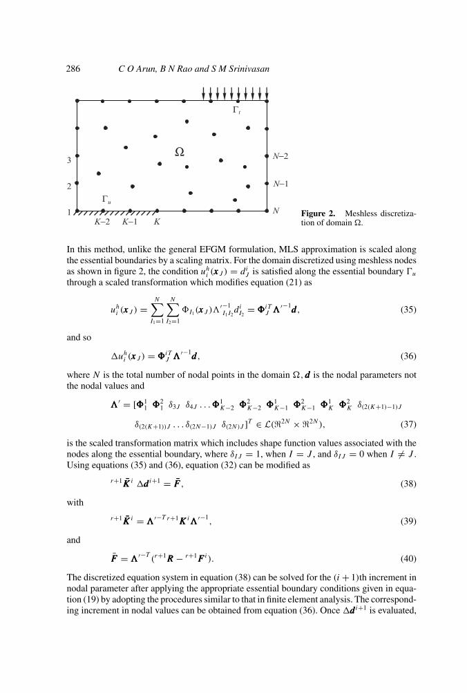
Figure 2. Meshless discretiza-tion of domain �.

In this method, unlike the general EFGM formulation, MLS approximation is scaled alongthe essential boundaries by a scaling matrix. For the domain discretized using meshless nodesas shown in figure 2, the condition uh

i (xxxJ ) = diJ is satisfied along the essential boundary u

through a scaled transformation which modifies equation (21) as

uhi (xxxJ ) =

N∑I1=1

N∑I2=1

�I1(xxxJ )�′−1I1I2

diI2

= ��iTJ ��′−1

ddd, (35)

and so

�uhi (xxxJ ) = ��iT

J ��′−1ddd, (36)

where N is the total number of nodal points in the domain �,ddd is the nodal parameters notthe nodal values and

��′ = [��11 ��2

1 δ3J δ4J . . .��1K−2 ��2

K−2 ��1K−1 ��2

K−1 ��1K ��2

K δ(2(K+1)−1)J

δ(2(K+1))J . . . δ(2N−1)J δ(2N)J ]T ∈ L(�2N × �2N), (37)

is the scaled transformation matrix which includes shape function values associated with thenodes along the essential boundary, where δIJ = 1, when I = J , and δIJ = 0 when I = J .Using equations (35) and (36), equation (32) can be modified as

r+1KKKi �dddi+1 = FFF , (38)

with

r+1KKKi = ��′−T r+1KKKi��′−1, (39)

and

FFF = ��′−T(r+1RRR − r+1FFF i). (40)

The discretized equation system in equation (38) can be solved for the (i + 1)th increment innodal parameter after applying the appropriate essential boundary conditions given in equa-tion (19) by adopting the procedures similar to that in finite element analysis. The correspond-ing increment in nodal values can be obtained from equation (36). Once �dddi+1 is evaluated,


the corresponding strain, stress and damage increment can be found out using the proceduredescribed further. During Newton–Raphson iteration, an inaccurate transition to plastic statemay occur especially if the load step is too large. This should result in large imbalance, andthe following iterations should in general be able to correct it. However, any plastic strainthat was accumulated during the iteration will still be there and in later iterations will give anerroneous yield stress (Bhatti 2006). To avoid this problem, instead of using the displacementincrement from the current iteration, the total displacement increment from the beginning ofthe current load step should be used. Thus

�dddi+1 =i+1∑i=1

�dddj . (41)

Then the total strain increment,

�εεεi+1 = BBBT��′−1�dddi+1. (42)

Once the strain increment is calculated, the other state variables like stress, plastic strain anddamage at the end of new load step is to be found. The state determination procedure is brieflyoutlined below.

3.3 Procedure for state determination

For a given Gauss point, with known increment in strain (�εεε), and the previous state(σσσ , εεε,χχχ, κ , and εεεp) the basic steps in computing a new state are as follows:

1. Compute the elastic predictor, and trial stress increment using,

�σσσ e = CCC�εεε

sss = σσσ + �σσσ e. (43)

2. Evaluate the yield function value f (sss,χχχ, κ). For a previously elastic Gauss point continuewith step 3, otherwise go to step 4.

3. For a previously elastic Gauss point, there are two possibilities,

(a) Gauss point remains to be elastic i.e. f (sss,χχχ, κ) ≤ 0 and r+1σσσ i+1 = sss and other statevariables, related to plastic part remains same as in the previous load step. Go to step 7.

(b) f (sss,χχχ, κ) > 0 with a transition from elastic to plastic state. Locate stress at yieldpoint by solving f (σσσ +ρ�σρ�σρ�σe,χχχ, κ) = 0 where ρ is the fraction of strain incrementthat takes the stress to yield stress level. ρ�εεε is the strain increment that takes stressto yield level and (1 − ρ)�εεε is called as elasto-plastic strain increment. Continue tostep 5.

4. For a previous yielded Gauss point there are three possibilities;

(a) It continues to yield plastically. Then ρ = 0 and continue to step 5.(b) It unloads elastically, with f (sss,χχχ, κ) ≤ 0. Then r+1σσσ i+1 = sss and go to step 7.(c) It unloads by moving inside the yield surface and eventually ends up with a stress out

side the yield surface, which requires to find ρ and then continue to step 5.


5. In this step the stresses corresponding to (1 − ρ)�εεε are to be found out. The availableliterature on damage mechanics uses the integration scheme proposed by Benallal et al1988, which requires an iteration for yield surface drift correction, to minimize the errorsthat arise due the replacement of differential quantities to finite difference quantities. Inthe present work a simple implicit scheme (Sivakumar & Voyiadjis 1997), which usessingle point integration without any iteration, is used. The final state for which the yieldcondition to be satisfied is used to obtain the discrete consistency condition,

f (σσσ + ρ�σσσ e + �σσσ ,χχχ + �χχχ, κ + �κ) = 0. (44)

For an associated flow rule, the evolution equations given in equations (11)–(14) can berewritten in incremental form as

�εεεp = �λ∂f

∂σσσ, (45)

�χχχ = −h�λ∂F

∂χχχ, (46)

�κ = −H�λ∂F

∂κ, (47)

�D = �λ∂FD

∂Y, (48)

where h and H are kinematic and isotropic hardening modulus respectively. The elasto-plastic constitutive equation can be written as

�σσσ = CCC(�εεε − �εεεp), (49)

where �εεε = (1 − ρ)�εεε. Substituting equations (45)–(49) into equation (44), will lead toa polynomial in �λ. For the von Mises yield criteria, which is used in the present study,the polynomial will be a quadratic equation in �λ with coefficients in terms of initialquantities (Sivakumar & Voyiadjis 1997). To solve the equation (44) for �λ and usingequations (45)–(49) update all the variables as

r+1σσσ i+1 = σσσ + ρ�σσσ e + �σσσ

r+1εεεi+1 = εεε + �εεε

r+1εεεpi+1 = εεεp + �εεεp

r+1χχχi+1 = χχχ + �χχχ

r+1κi+1 = κ + �κ

r+1Di+1 = D + �D. (50)

6. For an associated flow rule, the elasto-plastic stiffness matrix CCCep is evaluated at eachiteration using the method described by Chen & Han (1988).

7. Check for convergence with new state values. Force equilibrium and internal energycriteria can be used (Chen & Han 1988; Bhatti 2006). If the prescribed tolerance isachieved, Newton–Raphson iterations can be stopped and can be proceeded to the nextload step.


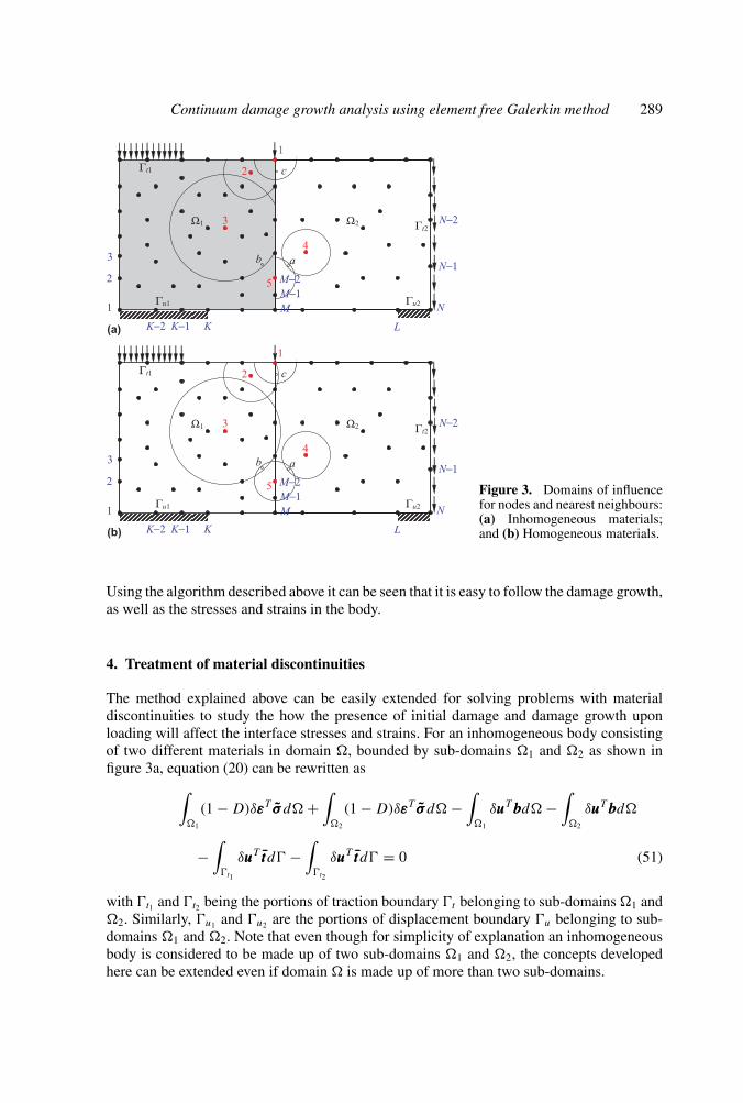
Figure 3. Domains of influencefor nodes and nearest neighbours:(a) Inhomogeneous materials;and (b) Homogeneous materials.

Using the algorithm described above it can be seen that it is easy to follow the damage growth,as well as the stresses and strains in the body.

4. Treatment of material discontinuities

The method explained above can be easily extended for solving problems with materialdiscontinuities to study the how the presence of initial damage and damage growth uponloading will affect the interface stresses and strains. For an inhomogeneous body consistingof two different materials in domain �, bounded by sub-domains �1 and �2 as shown infigure 3a, equation (20) can be rewritten as

∫�1

(1 − D)δεεεT σσσd� +∫

�2

(1 − D)δεεεT σσσd� −∫

�1

δuuuTbbbd� −∫

�2

δuuuTbbbd�

−∫

t1

δuuuT tttd −∫

t2

δuuuT tttd = 0 (51)

with t1 and t2 being the portions of traction boundary t belonging to sub-domains �1 and�2. Similarly, u1 and u2 are the portions of displacement boundary u belonging to sub-domains �1 and �2. Note that even though for simplicity of explanation an inhomogeneousbody is considered to be made up of two sub-domains �1 and �2, the concepts developedhere can be extended even if domain � is made up of more than two sub-domains.


The stiffness equation system is assembled in each of sub-domains separately, noting thatall points contained in material 1 can only be influenced by nodes in material 1 plus interfacenodes; and, all points contained in material 2 can only be influenced by nodes containedin material 2 plus interface nodes. Figures 3a and 3b, respectively illustrate the differencein selection of the neighbours to a point in domain �, when sub-domains �1 and �2 areconsidered to be of different materials (inhomogeneous materials) and when sub-domains �1

and �2are considered to be of same materials (homogeneous materials). When sub-domains�1 and �2 are considered to be of different materials, the domains of influence for nodescompletely inside sub-domains �1 and �2 are truncated at the interface, leaving the domainsof influence for an interface node belonging to both sub-domains �1 and �2 unaffected.

From equation (35), the MLS approximation of ui(xxxJ ) is

uhi (xxxJ ) =

M∑I1=1

M∑I2=1

�I1(xxxJ )�′(1)−1

I1I2di

I2= ��iT

J ��′(1)−1

ddd(1) if xxxJ ∈ �1

N∑I1=M−2

N∑I2=M−2

�I1(xxxJ )�′(2)−1

I1I2di

I2= ��iT

J ��′(2)−1

ddd(2) if xxxJ ∈ �2

, (52)

where

��′(1) = [��11 ��2

1 δJ3 δJ4 . . .��1K ��2

K δJ(2(K+1)−1) δJ (2(K+1)) . . .��1(M−2) ��2

(M−2)

��1(M−1) ��2

(M−1) ��1M ��2

M ]T ∈ L(�2M × �2M), (53)

and

��′(2) = [��1(M−2) ��2

(M−2) ��1(M−1) ��2

(M−1) . . . δJ (2(L−1)−1) δJ (2(L−1)) ��1L ��2

L

δJ(2(L+1)−1) δJ (2(L+1)) . . .��1(N−1) ��2

(N−1) ��1N ��2

N ]T

∈ L(�2(N−M) × �2(N−M)), (54)

are the scaled transformation matrices for the domains �1 and �2 respectively. Using equa-tion (52), by following the similar procedures as explained in section 4·1, stiffness equationsystem similar to equation (38) can be formulated for each of the sub-domains and can beassembled along the interface nodes to get the global stiffness equation system (Arun et al2009) and can solve for the increment in nodal parameters and strain increment in each of thesub-domains. The state determination procedure is similar to the one explained in section 4·2,except that for each of the sub-domains it has to be evaluated separately.

5. Numerical examples

To demonstrate the performance of EFGM described above, three numerical examples arepresented. In all the numerical examples material is treated as linear elastic, linear kinematichardening. The linear basis with the student’s t-distribution weight function (Rao & Rahman2000) is adopted in EFGM analysis. The scaling parameter, zmax (Rao & Rahman 2000)and the student’s t-distribution weight function (Rao & Rahman 2000) parameter, β aretaken as 2·01. For numerical integration, one point and 8 × 8 Gauss quadrature is adoptedrespectively for one and two-dimensional numerical examples presented below. Numericalexamples involving both with and without material discontinuities are solved.


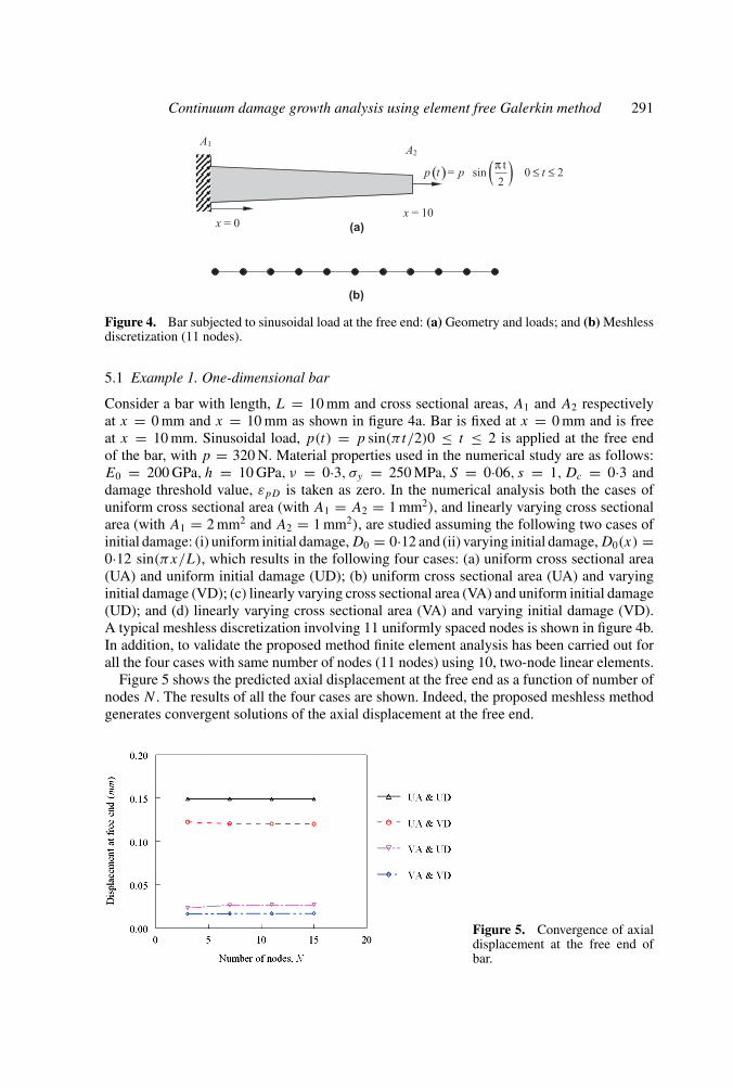
Figure 4. Bar subjected to sinusoidal load at the free end: (a) Geometry and loads; and (b) Meshlessdiscretization (11 nodes).

5.1 Example 1. One-dimensional bar

Consider a bar with length, L = 10 mm and cross sectional areas, A1 and A2 respectivelyat x = 0 mm and x = 10 mm as shown in figure 4a. Bar is fixed at x = 0 mm and is freeat x = 10 mm. Sinusoidal load, p(t) = p sin(πt/2)0 ≤ t ≤ 2 is applied at the free endof the bar, with p = 320 N. Material properties used in the numerical study are as follows:E0 = 200 GPa, h = 10 GPa, ν = 0·3, σy = 250 MPa, S = 0·06, s = 1, Dc = 0·3 anddamage threshold value, εpD is taken as zero. In the numerical analysis both the cases ofuniform cross sectional area (with A1 = A2 = 1 mm2), and linearly varying cross sectionalarea (with A1 = 2 mm2 and A2 = 1 mm2), are studied assuming the following two cases ofinitial damage: (i) uniform initial damage, D0 = 0·12 and (ii) varying initial damage, D0(x) =0·12 sin(πx/L), which results in the following four cases: (a) uniform cross sectional area(UA) and uniform initial damage (UD); (b) uniform cross sectional area (UA) and varyinginitial damage (VD); (c) linearly varying cross sectional area (VA) and uniform initial damage(UD); and (d) linearly varying cross sectional area (VA) and varying initial damage (VD).A typical meshless discretization involving 11 uniformly spaced nodes is shown in figure 4b.In addition, to validate the proposed method finite element analysis has been carried out forall the four cases with same number of nodes (11 nodes) using 10, two-node linear elements.

Figure 5 shows the predicted axial displacement at the free end as a function of number ofnodes N . The results of all the four cases are shown. Indeed, the proposed meshless methodgenerates convergent solutions of the axial displacement at the free end.

Figure 5. Convergence of axialdisplacement at the free end ofbar.


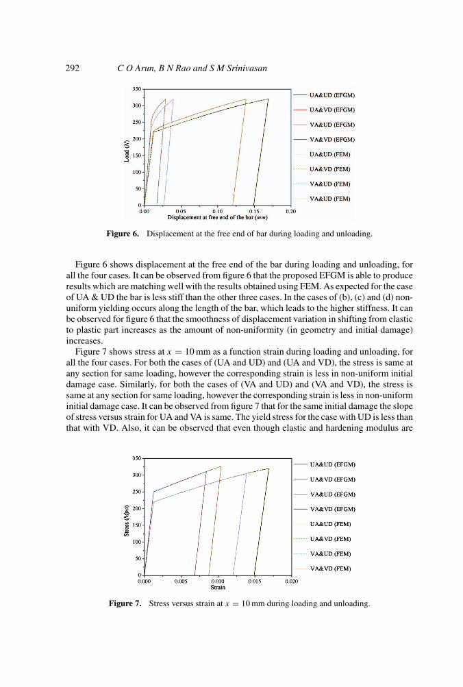
Figure 6. Displacement at the free end of bar during loading and unloading.

Figure 6 shows displacement at the free end of the bar during loading and unloading, forall the four cases. It can be observed from figure 6 that the proposed EFGM is able to produceresults which are matching well with the results obtained using FEM. As expected for the caseof UA & UD the bar is less stiff than the other three cases. In the cases of (b), (c) and (d) non-uniform yielding occurs along the length of the bar, which leads to the higher stiffness. It canbe observed for figure 6 that the smoothness of displacement variation in shifting from elasticto plastic part increases as the amount of non-uniformity (in geometry and initial damage)increases.

Figure 7 shows stress at x = 10 mm as a function strain during loading and unloading, forall the four cases. For both the cases of (UA and UD) and (UA and VD), the stress is same atany section for same loading, however the corresponding strain is less in non-uniform initialdamage case. Similarly, for both the cases of (VA and UD) and (VA and VD), the stress issame at any section for same loading, however the corresponding strain is less in non-uniforminitial damage case. It can be observed from figure 7 that for the same initial damage the slopeof stress versus strain for UA and VA is same. The yield stress for the case with UD is less thanthat with VD. Also, it can be observed that even though elastic and hardening modulus are

Figure 7. Stress versus strain at x = 10 mm during loading and unloading.


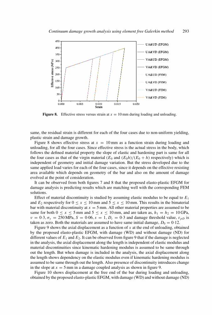
Figure 8. Effective stress versus strain at x = 10 mm during loading and unloading.

same, the residual strain is different for each of the four cases due to non-uniform yielding,plastic strain and damage growth.

Figure 8 shows effective stress at x = 10 mm as a function strain during loading andunloading, for all the four cases. Since effective stress is the actual stress in the body, whichfollows the defined material property the slope of elastic and hardening part is same for allthe four cases as that of the virgin material (E0 and (E0h)/(E0 + h) respectively) which isindependent of geometry and initial damage variation. But the stress developed due to thesame applied load varies for each of the four cases, since it depends on the effective resistingarea available which depends on geometry of the bar and also on the amount of damageevolved at the point of consideration.

It can be observed from both figures 7 and 8 that the proposed elasto-plastic EFGM fordamage analysis is predicting results which are matching well with the corresponding FEMsolutions.

Effect of material discontinuity is studied by assuming elastic modulus to be equal to E1

and E2 respectively for 0 ≤ x ≤ 10 mm and 5 ≤ x ≤ 10 mm. This results in the bimaterialbar with material discontinuity at x = 5 mm. All other material properties are assumed to besame for both 0 ≤ x ≤ 5 mm and 5 ≤ x ≤ 10 mm, and are taken as, h1 = h2 = 10 GPa,ν = 0·3, σy = 250 MPa, S = 0·06, s = 1, Dc = 0·3 and damage threshold value, εpD istaken as zero. Both the materials are assumed to have same initial damage, D0 = 0·12.

Figure 9 shows the axial displacement as a function of x at the end of unloading, obtainedby the proposed elasto-plastic EFGM, with damage (WD) and without damage (ND) fordifferent values of E1 and E2. It can be observed from figure 9 that if the damage is neglectedin the analysis, the axial displacement along the length is independent of elastic modulus andmaterial discontinuities since kinematic hardening modulus is assumed to be same throughout the length. But when damage is included in the analysis, the axial displacement alongthe length shows dependency on the elastic modulus even if kinematic hardening modulus isassumed to be same through out the length. Also presence of discontinuity introduces changein the slope at x = 5 mm in a damage coupled analysis as shown in figure 9.

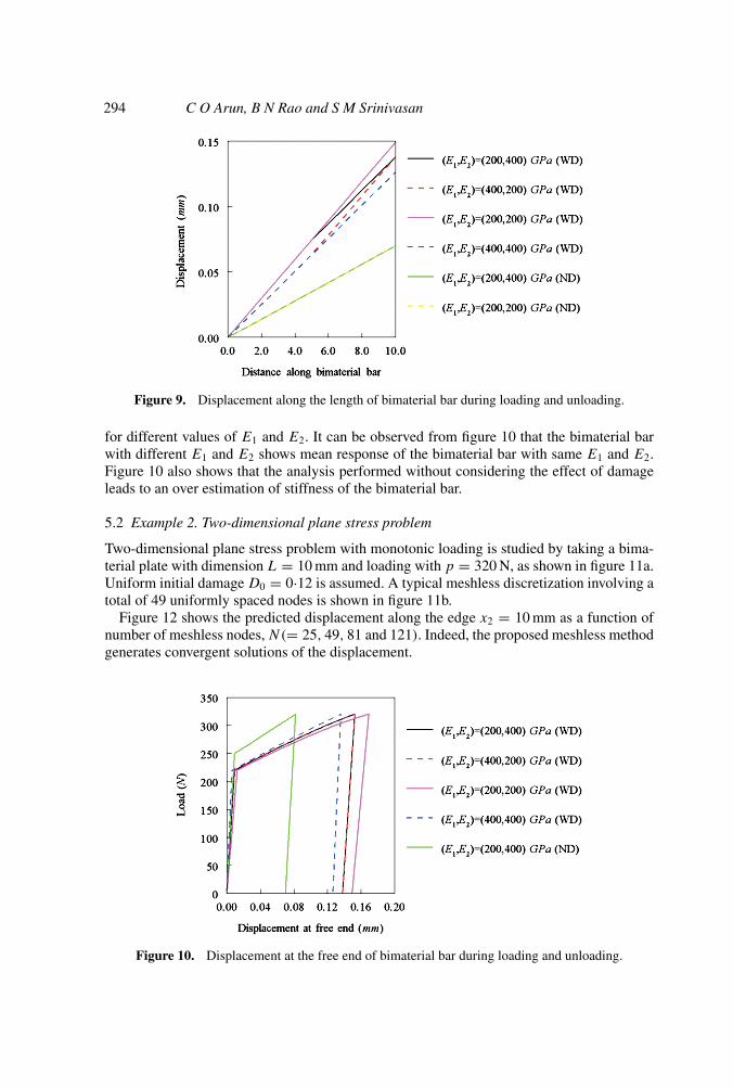
Figure 10 shows displacement at the free end of the bar during loading and unloading,obtained by the proposed elasto-plastic EFGM, with damage (WD) and without damage (ND)


Figure 9. Displacement along the length of bimaterial bar during loading and unloading.

for different values of E1 and E2. It can be observed from figure 10 that the bimaterial barwith different E1 and E2 shows mean response of the bimaterial bar with same E1 and E2.Figure 10 also shows that the analysis performed without considering the effect of damageleads to an over estimation of stiffness of the bimaterial bar.

5.2 Example 2. Two-dimensional plane stress problem

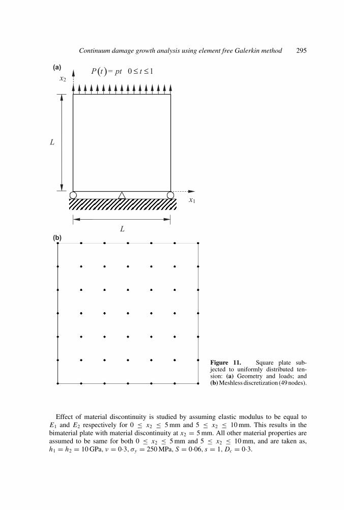
Two-dimensional plane stress problem with monotonic loading is studied by taking a bima-terial plate with dimension L = 10 mm and loading with p = 320 N, as shown in figure 11a.Uniform initial damage D0 = 0·12 is assumed. A typical meshless discretization involving atotal of 49 uniformly spaced nodes is shown in figure 11b.

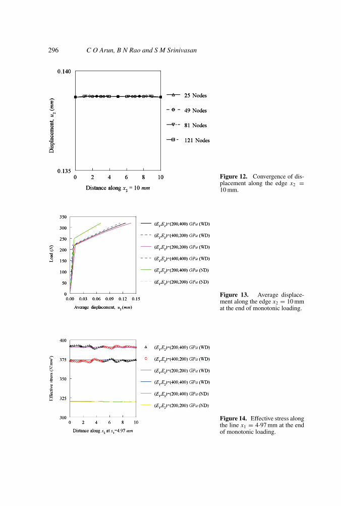
Figure 12 shows the predicted displacement along the edge x2 = 10 mm as a function ofnumber of meshless nodes, N(= 25, 49, 81 and 121). Indeed, the proposed meshless methodgenerates convergent solutions of the displacement.

Figure 10. Displacement at the free end of bimaterial bar during loading and unloading.


Figure 11. Square plate sub-jected to uniformly distributed ten-sion: (a) Geometry and loads; and(b) Meshless discretization (49 nodes).

Effect of material discontinuity is studied by assuming elastic modulus to be equal toE1 and E2 respectively for 0 ≤ x2 ≤ 5 mm and 5 ≤ x2 ≤ 10 mm. This results in thebimaterial plate with material discontinuity at x2 = 5 mm. All other material properties areassumed to be same for both 0 ≤ x2 ≤ 5 mm and 5 ≤ x2 ≤ 10 mm, and are taken as,h1 = h2 = 10 GPa, ν = 0·3, σy = 250 MPa, S = 0·06, s = 1, Dc = 0·3.


Figure 12. Convergence of dis-placement along the edge x2 =10 mm.

Figure 13. Average displace-ment along the edge x2 = 10 mmat the end of monotonic loading.

Figure 14. Effective stress alongthe line x1 = 4·97 mm at the endof monotonic loading.


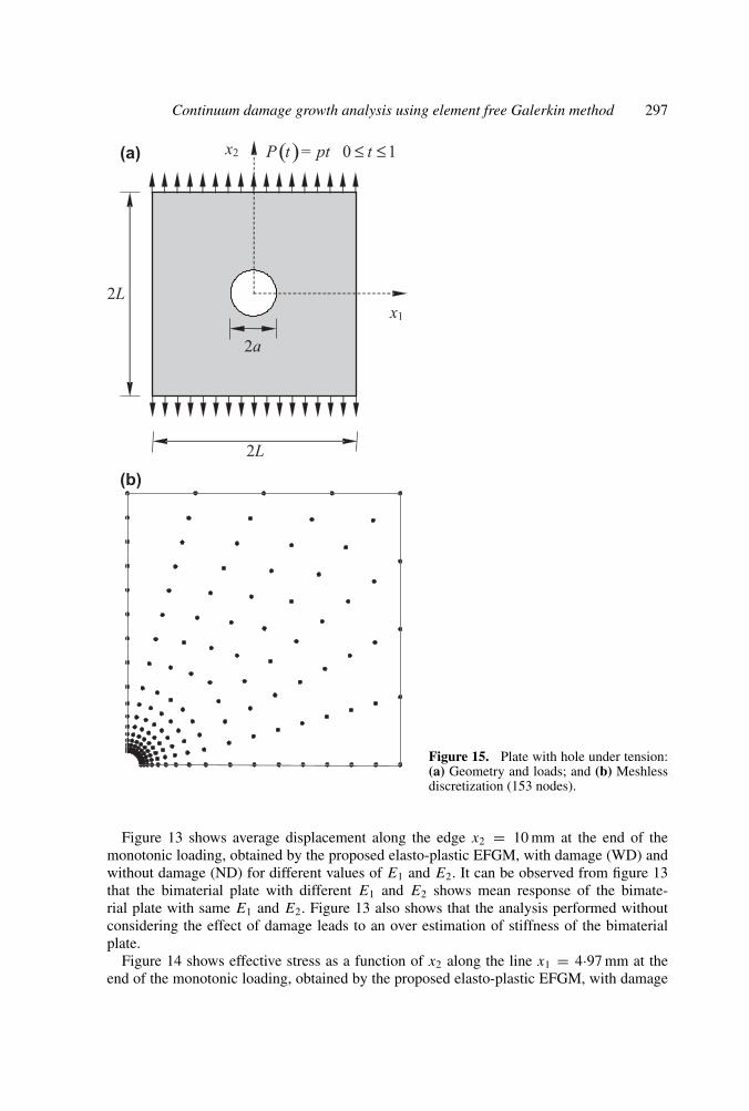
Figure 15. Plate with hole under tension:(a) Geometry and loads; and (b) Meshlessdiscretization (153 nodes).

Figure 13 shows average displacement along the edge x2 = 10 mm at the end of themonotonic loading, obtained by the proposed elasto-plastic EFGM, with damage (WD) andwithout damage (ND) for different values of E1 and E2. It can be observed from figure 13that the bimaterial plate with different E1 and E2 shows mean response of the bimate-rial plate with same E1 and E2. Figure 13 also shows that the analysis performed withoutconsidering the effect of damage leads to an over estimation of stiffness of the bimaterialplate.

Figure 14 shows effective stress as a function of x2 along the line x1 = 4·97 mm at theend of the monotonic loading, obtained by the proposed elasto-plastic EFGM, with damage


(WD) and without damage (ND) for different values of E1 and E2. It can be observed fromfigure 14 that material discontinuity results in effective stress jump at the interface. Differentvalues of E1 and E2 resulted oscillations in predicted effective stress. These oscillations inpredicted effective stress are observed to be reduced with increased refinement of meshlessdiscretization. From figure 14 it can be observed that in the analysis without consideringdamage effective stress is same as stress and that the stress equilibrium across the interfaceis satisfied as expected.

5.3 Example 3. Plate with a hole under tension

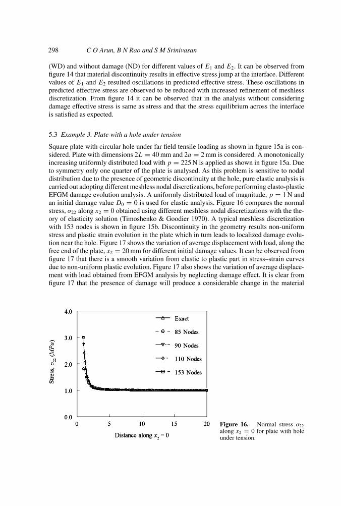
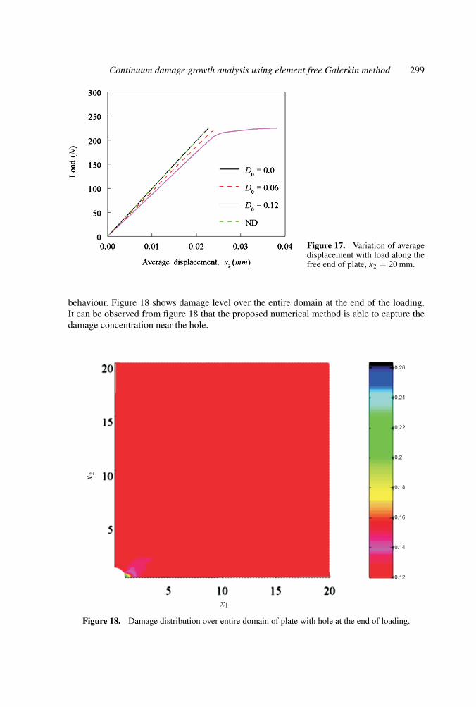
Square plate with circular hole under far field tensile loading as shown in figure 15a is con-sidered. Plate with dimensions 2L = 40 mm and 2a = 2 mm is considered. A monotonicallyincreasing uniformly distributed load with p = 225 N is applied as shown in figure 15a. Dueto symmetry only one quarter of the plate is analysed. As this problem is sensitive to nodaldistribution due to the presence of geometric discontinuity at the hole, pure elastic analysis iscarried out adopting different meshless nodal discretizations, before performing elasto-plasticEFGM damage evolution analysis. A uniformly distributed load of magnitude, p = 1 N andan initial damage value D0 = 0 is used for elastic analysis. Figure 16 compares the normalstress, σ22 along x2 = 0 obtained using different meshless nodal discretizations with the the-ory of elasticity solution (Timoshenko & Goodier 1970). A typical meshless discretizationwith 153 nodes is shown in figure 15b. Discontinuity in the geometry results non-uniformstress and plastic strain evolution in the plate which in tum leads to localized damage evolu-tion near the hole. Figure 17 shows the variation of average displacement with load, along thefree end of the plate, x2 = 20 mm for different initial damage values. It can be observed fromfigure 17 that there is a smooth variation from elastic to plastic part in stress–strain curvesdue to non-uniform plastic evolution. Figure 17 also shows the variation of average displace-ment with load obtained from EFGM analysis by neglecting damage effect. It is clear fromfigure 17 that the presence of damage will produce a considerable change in the material

Figure 16. Normal stress σ22along x2 = 0 for plate with holeunder tension.


Figure 17. Variation of averagedisplacement with load along thefree end of plate, x2 = 20 mm.

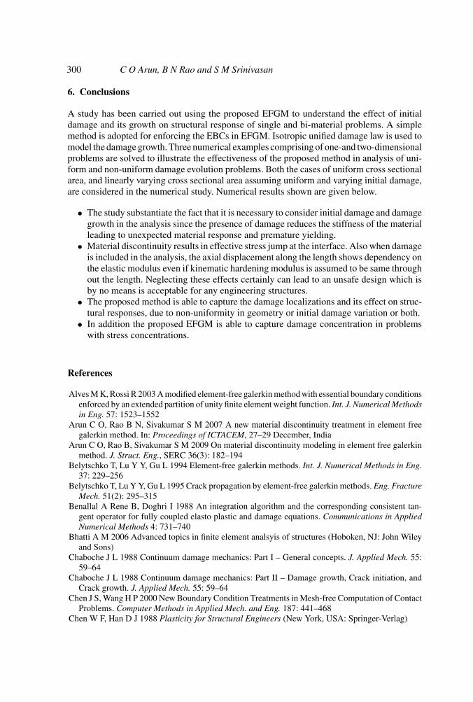
behaviour. Figure 18 shows damage level over the entire domain at the end of the loading.It can be observed from figure 18 that the proposed numerical method is able to capture thedamage concentration near the hole.

Figure 18. Damage distribution over entire domain of plate with hole at the end of loading.


6. Conclusions

A study has been carried out using the proposed EFGM to understand the effect of initialdamage and its growth on structural response of single and bi-material problems. A simplemethod is adopted for enforcing the EBCs in EFGM. Isotropic unified damage law is used tomodel the damage growth. Three numerical examples comprising of one-and two-dimensionalproblems are solved to illustrate the effectiveness of the proposed method in analysis of uni-form and non-uniform damage evolution problems. Both the cases of uniform cross sectionalarea, and linearly varying cross sectional area assuming uniform and varying initial damage,are considered in the numerical study. Numerical results shown are given below.

• The study substantiate the fact that it is necessary to consider initial damage and damagegrowth in the analysis since the presence of damage reduces the stiffness of the materialleading to unexpected material response and premature yielding.

• Material discontinuity results in effective stress jump at the interface. Also when damageis included in the analysis, the axial displacement along the length shows dependency onthe elastic modulus even if kinematic hardening modulus is assumed to be same throughout the length. Neglecting these effects certainly can lead to an unsafe design which isby no means is acceptable for any engineering structures.

• The proposed method is able to capture the damage localizations and its effect on struc-tural responses, due to non-uniformity in geometry or initial damage variation or both.

• In addition the proposed EFGM is able to capture damage concentration in problemswith stress concentrations.

References

Alves M K, Rossi R 2003 A modified element-free galerkin method with essential boundary conditionsenforced by an extended partition of unity finite element weight function. Int. J. Numerical Methodsin Eng. 57: 1523–1552

Arun C O, Rao B N, Sivakumar S M 2007 A new material discontinuity treatment in element freegalerkin method. In: Proceedings of ICTACEM, 27–29 December, India

Arun C O, Rao B, Sivakumar S M 2009 On material discontinuity modeling in element free galerkinmethod. J. Struct. Eng., SERC 36(3): 182–194

Belytschko T, Lu Y Y, Gu L 1994 Element-free galerkin methods. Int. J. Numerical Methods in Eng.37: 229–256

Belytschko T, Lu Y Y, Gu L 1995 Crack propagation by element-free galerkin methods. Eng. FractureMech. 51(2): 295–315

Benallal A Rene B, Doghri I 1988 An integration algorithm and the corresponding consistent tan-gent operator for fully coupled elasto plastic and damage equations. Communications in AppliedNumerical Methods 4: 731–740

Bhatti A M 2006 Advanced topics in finite element analsyis of structures (Hoboken, NJ: John Wileyand Sons)

Chaboche J L 1988 Continuum damage mechanics: Part I – General concepts. J. Applied Mech. 55:59–64

Chaboche J L 1988 Continuum damage mechanics: Part II – Damage growth, Crack initiation, andCrack growth. J. Applied Mech. 55: 59–64

Chen J S, Wang H P 2000 New Boundary Condition Treatments in Mesh-free Computation of ContactProblems. Computer Methods in Applied Mech. and Eng. 187: 441–468

Chen W F, Han D J 1988 Plasticity for Structural Engineers (New York, USA: Springer-Verlag)


Dolbow J, Belytschko T 1998 An introduction to programming the meshless element free galerkinmethod. Archives of Computational Mechanics 15(3): 207–241

Duarte C A M, Oden J T 1996 H − p Clouds – An h − p meshless method. Numerical Methods forPartial Differential Equations 12(6): 673–705

Kachanov L M 1958 Time of the rupture process under creep conditions. IVZ Akad Nauk,S. S. R. Otd Tecg Bayj, 8: 26–31

Kattan P I, Voyiadjis G Z 2002 Damage mechanics with finite elements practical applications withcomputer tools (Berlin, Heidelberg, Germany: Springer-Verlag)

Krongauz Y, Belytschko T 1996 Enforcement of essential boundary conditions in meshless approxi-mation using finite elements. Computer Methods in Applied Mechanics and Eng. 131: 1335–1345

Lancaster P, Salkauskas K 1981 Surfaces generated by moving least squares methods. Mathematicsof Computation 37: 141–158

Lemaitre J 1971 Evaluation and dissipation of damage in metals submitted to dynamic loading. In:Proceedings I.C.M.I. Kyoto, Japan

Lemaitre J 1985 A continuous damage mechanics model for ductile fracture. J. Eng. Materials andTechnol. 107: 83–89

Lemaitre J 1992 A course on damage mechanics (Berlin, Heidelberg, Germany: Springer-Verlag)Lemaitre J, Desmorat R 2005 Engineering damage mechanics (Berlin, Heidelberg, Germany:

Springer-Verlag)Liu W K, Jun S, Zhang Y F 1995 Reproducing kernel particle methods. Int. J. Numerical Methods in

Fluids 20: 1081–1106Liu W K, Li S, Belytschko T 1997 Moving least square kernel galerkin method – Part I: Methodology

and convergence. Computer Methods in Applied Mechanics and Eng. 143: 422–433Liu G R 2002 Mesh free methods: Moving beyond the finite element method (LLC, Boca Raton FL,

USA: CRC Press)Li G, Belytschko T 2001 Element-free galerkin methods for contact problems in metal forming

analysis. Eng. Computations 18: 62–78Lucy L 1977 A numerical approach to testing the fission hypothesis. Astron. J. 82: 1013–1024Lu Y Y, Belytschko T, Gu L 1994 A new implementation of the element free galerkin method.

Computer Methods in Applied Mechanics and Eng. 113: 397–414Lu Y Y, Belytschko T, Tabbara M 1995 Element-free galerkin methods for wave propagation and

dynamic fracture. Computer Methods in Applied Mechanics and Eng. 126: 131–153Melenk J M, Babuska I 1996 The partition of unity finite element method: Basic theory and applica-

tions. Computer Methods in Applied Mechanics and Eng. 139: 280–314Monaghan J J 1988 An introduction to SPH. Computer Physics Communications 48: 89–96Nagashima T 1999 Node-by-Node meshless approach and its applications to structural analyses. Int.

J. Numerical Methods in Eng. 46: 341–385Nayroles B, Touzot G, Villon P 1992 Generalizing the finite element method: Diffuse approximation

and diffuse elements. Computational Mechanics 10: 307–318Ponthot J P, Belytschko T 1998 Arbitrary lagrangian-eulerian formulation for element-free galerkin

method. Computer Methods in Applied Mechanics and Eng. 152: 19–46Rabotnov Y N 1969 Creep Problems of Structural Members. (North Holland, Amsterdam)Rao B N, Rahman S 2000 An efficient meshless method for fracture analysis of cracks. Computational

Mechanics 26(4): 398–408Sivakumar M S, Voyiadjis G Z 1997 A simple implicit scheme for stress response computation in

plasticity models. Computational Mechanics 20: 520–529Timoshenko S P, Goodier J N 1970 Theory of Elasticity. (New York, USA: McGraw-Hill)Voyiadjis G Z, Kattan P I 1990 A coupled theory of dmage mechanics and finite strain elasto-plasticity-

II. Damage and Finite Strain Plasticity. Int. J. Eng. Sci. 28(6): 505–524Voyiadjis G Z, Kattan P I 2005 Damage mechanics (LLC, Boca Raton FL, USA: CRC Press)

Documents

Continuum damage growth analysis using …apm.iitm.ac.in/smlab/mss/download/52.pdfContinuum damage growth analysis using element free Galerkin method 281 Figure 1. Mechanical representation