CONTOURSA Mathematical Coloring Book

ALEXANDER RAICHEV

Introduction

Q: What is this?A: This is a mathematical coloring book. It contains black and white pictures generated

by mathematical formulas which you color in for fun.Q: Why did you make it?A: I like math and drawing and decided to combine the two. Also, I was inspired by

[Ham].Q: Is this book for kids or adults?A: Both. The only requirements are sharp pencils and fine motor skills.Q: What does the title mean?A: Every picture in this book is a contour plot. A contour plot of a three-dimensional

object is an overlay of several parallel two-dimensional cross sections of the object, eachof which is called a contour line or contour. You can think of the object as a landscapeand the contour plot as a topographical map of that landscape.

Q: How did you make these pictures?A: For each picture I chose a function from the plane to the plane, computed several

of its iterates, collapsed the outputs to the real line, plotted one to three contours ofthe resulting functions, overlaid them, and then cropped and sometimes rotated andresized the result. I got this idea from [Ham]. To make the plots, I used Sage [S+13], anopen-source mathematics software system.

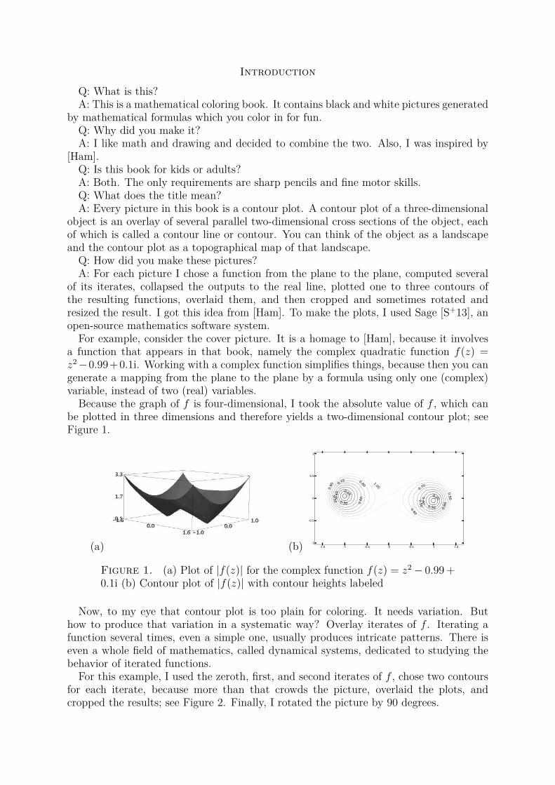
For example, consider the cover picture. It is a homage to [Ham], because it involvesa function that appears in that book, namely the complex quadratic function f(z) =z2−0.99+0.1i. Working with a complex function simplifies things, because then you cangenerate a mapping from the plane to the plane by a formula using only one (complex)variable, instead of two (real) variables.

Because the graph of f is four-dimensional, I took the absolute value of f , which canbe plotted in three dimensions and therefore yields a two-dimensional contour plot; seeFigure 1.

(a) (b) -1.5 -1 -0.5 0 0.5 1 1.5-1

-0.5

0

0.5

1

0.20

0.20

0.30

0.30

0.4

0

0.4

0

0.5

0

0.5

0

0.6

00.6

0

0.700.70

0.80

0.80

0.9

0

0.90

1.00

Figure 1. (a) Plot of |f(z)| for the complex function f(z) = z2− 0.99 +0.1i (b) Contour plot of |f(z)| with contour heights labeled

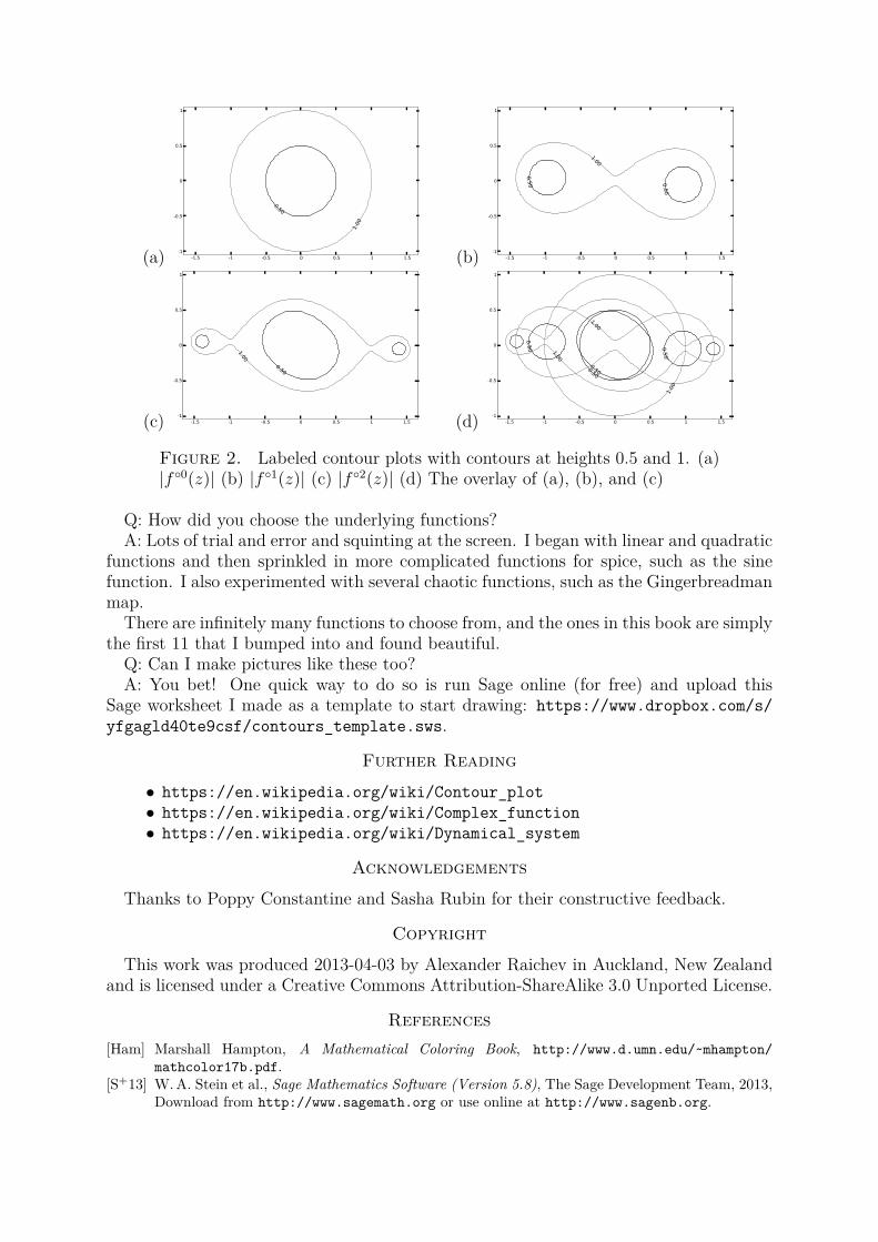
Now, to my eye that contour plot is too plain for coloring. It needs variation. Buthow to produce that variation in a systematic way? Overlay iterates of f . Iterating afunction several times, even a simple one, usually produces intricate patterns. There iseven a whole field of mathematics, called dynamical systems, dedicated to studying thebehavior of iterated functions.

For this example, I used the zeroth, first, and second iterates of f , chose two contoursfor each iterate, because more than that crowds the picture, overlaid the plots, andcropped the results; see Figure 2. Finally, I rotated the picture by 90 degrees.

(a) -1.5 -1 -0.5 0 0.5 1 1.5-1

-0.5

0

0.5

1

0.50

1.00

(b) -1.5 -1 -0.5 0 0.5 1 1.5-1

-0.5

0

0.5

1

0.5

0

0.5

0

1.00

(c) -1.5 -1 -0.5 0 0.5 1 1.5-1

-0.5

0

0.5

1

0.50

1.00

(d) -1.5 -1 -0.5 0 0.5 1 1.5-1

-0.5

0

0.5

1

0.50

1.00

0.5

0

0.5

0

1.00

0.50

1.00

Figure 2. Labeled contour plots with contours at heights 0.5 and 1. (a)|f ◦0(z)| (b) |f ◦1(z)| (c) |f ◦2(z)| (d) The overlay of (a), (b), and (c)

Q: How did you choose the underlying functions?A: Lots of trial and error and squinting at the screen. I began with linear and quadratic

functions and then sprinkled in more complicated functions for spice, such as the sinefunction. I also experimented with several chaotic functions, such as the Gingerbreadmanmap.

There are infinitely many functions to choose from, and the ones in this book are simplythe first 11 that I bumped into and found beautiful.

Q: Can I make pictures like these too?A: You bet! One quick way to do so is run Sage online (for free) and upload this

Sage worksheet I made as a template to start drawing: https://www.dropbox.com/s/yfgagld40te9csf/contours_template.sws.

Further Reading

• https://en.wikipedia.org/wiki/Contour_plot• https://en.wikipedia.org/wiki/Complex_function• https://en.wikipedia.org/wiki/Dynamical_system

Acknowledgements

Thanks to Poppy Constantine and Sasha Rubin for their constructive feedback.

Copyright

This work was produced 2013-04-03 by Alexander Raichev in Auckland, New Zealandand is licensed under a Creative Commons Attribution-ShareAlike 3.0 Unported License.

References[Ham] Marshall Hampton, A Mathematical Coloring Book, http://www.d.umn.edu/~mhampton/

mathcolor17b.pdf.[S+13] W. A. Stein et al., Sage Mathematics Software (Version 5.8), The Sage Development Team, 2013,

Download from http://www.sagemath.org or use online at http://www.sagenb.org.

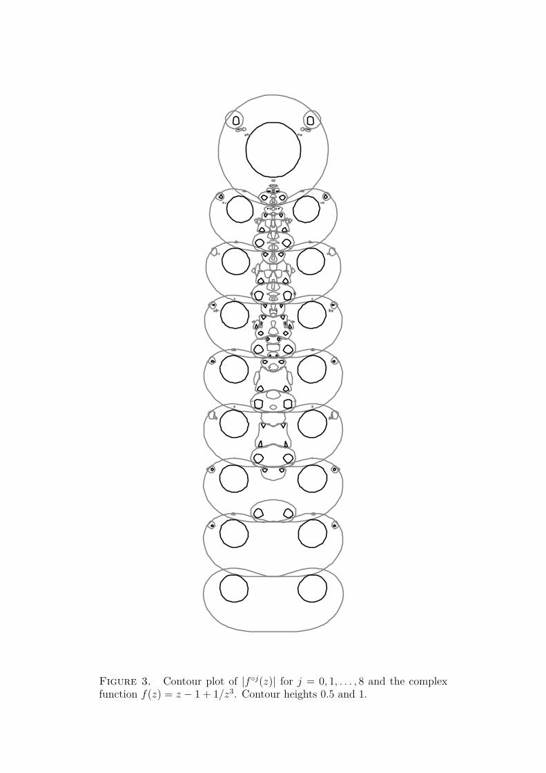
Figure 3. Contour plot of |f ◦j(z)| for j = 0, 1, . . . , 8 and the complexfunction f(z) = z − 1 + 1/z3. Contour heights 0.5 and 1.

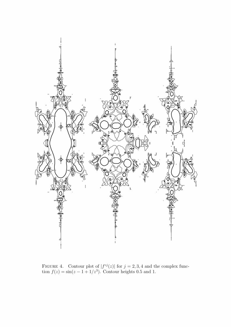
Figure 4. Contour plot of |f ◦j(z)| for j = 2, 3, 4 and the complex func-tion f(z) = sin(z − 1 + 1/z3). Contour heights 0.5 and 1.

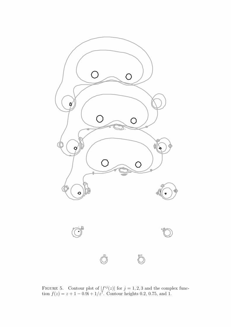
Figure 5. Contour plot of |f ◦j(z)| for j = 1, 2, 3 and the complex func-tion f(z) = z + 1− 0.9i + 1/z7. Contour heights 0.2, 0.75, and 1.

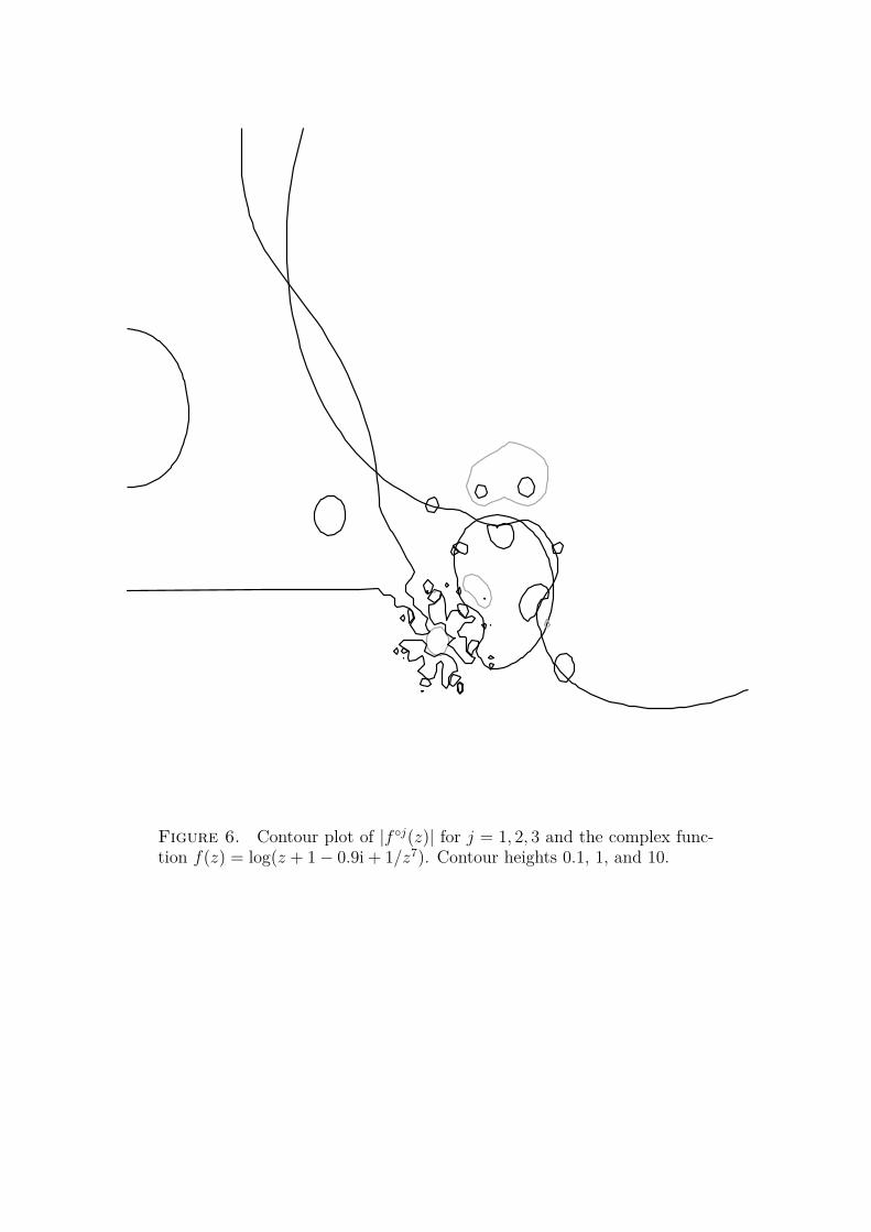
Figure 6. Contour plot of |f ◦j(z)| for j = 1, 2, 3 and the complex func-tion f(z) = log(z + 1− 0.9i + 1/z7). Contour heights 0.1, 1, and 10.

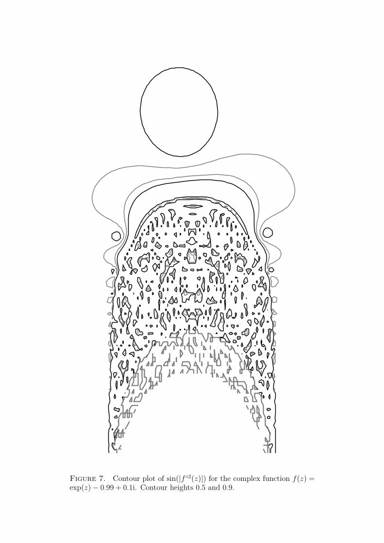
Figure 7. Contour plot of sin(|f ◦2(z)|) for the complex function f(z) =exp(z)− 0.99 + 0.1i. Contour heights 0.5 and 0.9.

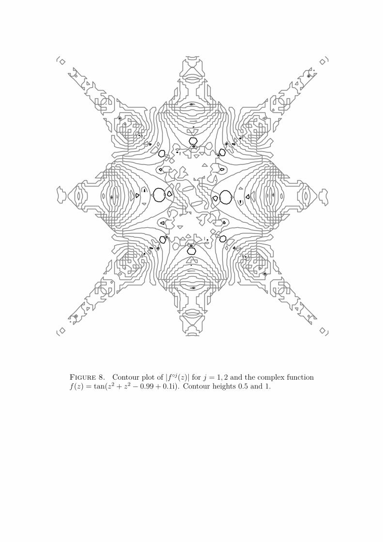
Figure 8. Contour plot of |f ◦j(z)| for j = 1, 2 and the complex functionf(z) = tan(z2 + z2 − 0.99 + 0.1i). Contour heights 0.5 and 1.

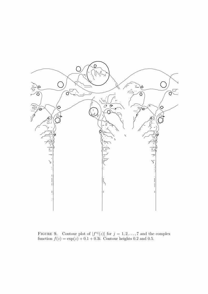
Figure 9. Contour plot of |f ◦j(z)| for j = 1, 2, . . . , 7 and the complexfunction f(z) = exp(z) + 0.1 + 0.3i. Contour heights 0.2 and 0.5.

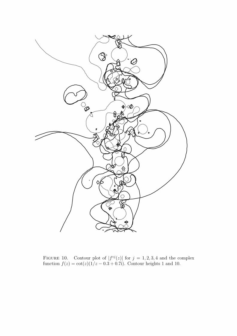
Figure 10. Contour plot of |f ◦j(z)| for j = 1, 2, 3, 4 and the complexfunction f(z) = cot(z)(1/z − 0.3 + 0.7i). Contour heights 1 and 10.

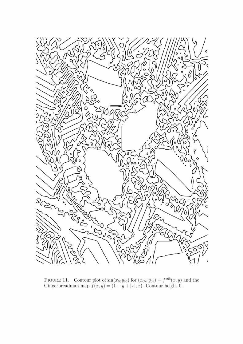
Figure 11. Contour plot of sin(x65y65) for (x65, y65) = f ◦65(x, y) and theGingerbreadman map f(x, y) = (1− y + |x|, x). Contour height 0.

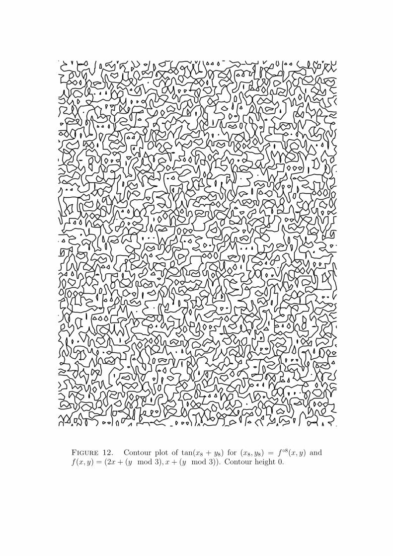
Figure 12. Contour plot of tan(x8 + y8) for (x8, y8) = f ◦8(x, y) andf(x, y) = (2x + (y mod 3), x + (y mod 3)). Contour height 0.