Contracting for Soil Carbon Credits: Design and Costs of Measurement and Monitoring

Siân Mooney1 John Antle

Susan Capalbo and

Keith Paustian2

Staff Paper 2002-01 May 9, 2002

American Agricultural Economics Association 2002 Annual Meeting July 28-31, 2002, Long Beach, California

Preliminary draft. Comments welcome.

Corresponding Author: Siân Mooney Dept. Agricultural Economics and Economics Montana State University PO Box 172920 Bozeman, Montana 59717-2920 Phone: 406-994-3036 Fax: 406-994-4838

E-mail: smooney@montana.edu

Funded by Montana Agricultural Experiment Station – series #2002-29, USDA/NRICGP grant #427430 and the National Science Foundation grant #427139.

1Resarch Assistant Professor; Professor and University Fellow, Resources For the Future; and Professor respectively, Department of Agricultural Economics and Economics, Montana State University, Bozeman, Montana 59717. 2Professor, Natural Resource Ecology Laboratory, Colorado State University, Fort Collins, Colorado 80523.

Copyright 2002 by Siân Mooney, John Antle, Susan Capalbo and Keith Paustian. All rights reserved. Readers may make verbatim copies of this document for non-commercial purposes by any means, provided that this copyright notice appears on all such copies.

Abstract

Many firms anticipate that a cap on greenhouse gas emissions will eventually be imposed, either through an international agreement like the Kyoto protocol or through domestic policy, and have started to take voluntary actions to reduce their emissions. If agricultural producers participate in the emerging market for tradable C-credits, it must be possible to verify that actions farmers take do increase the amount of C in soils and this increase can be maintained over the length of the contract.

In this paper we develop a prototype measurement and monitoring scheme for C-credits sequestered in agricultural soils and estimate its costs for the small grain-producing region of Montana using an econometric-process simulation model. Three key results emerge from the prototype framework. First, the efficiency of measurement and monitoring procedures for agricultural soil C sequestration depends on the price of C credits. Second, we find that at all price levels, costs of measuring and monitoring are largest in areas that exhibit the greatest heterogeneity in carbon values. Third, in a case study application of our prototype measurement and monitoring scheme, we find that if we assume similar error and confidence levels as forestry contracts, the upper estimate of measurement and monitoring costs associated with a contract that pays farmers per tonne of C sequestered is 3% of the value of a C-credit. This cost is small relative to the estimated net value of the contract. Thus we conclude that measurement and monitoring costs are not likely to be large enough to prevent producers from participating in a market for tradable credits.

Contracting for Soil Carbon Credits: Design and Costs of Measurement and Monitoring

Introduction and rationale

Many industrialized counties are considering ways to reduce their net emissions of

greenhouse gases (GHG), such as carbon dioxide, that potentially contribute to global warming

(Watson et al. 1996). The Kyoto protocol of the United Nations Framework Convention on

Climate Change is part of an ongoing international discussion that aims to identify means of

reducing GHG (UNFCCC 1998). One proposal is a C (carbon) credit-trading scheme that would

allow participating countries to receive credits for domestic or international projects that reduce

emissions beyond a “business as usual” case. In 2001, the Bush administration announced that it

would not sign the Kyoto protocol but in February 2002 announced a global climate change

initiative that proposed to include forest and agricultural soil C sequestration in U.S.

conservation programs and to develop accounting rules for sequestration projects (White House

2002). While the Bush climate change initiative is voluntary, the document acknowledged that

limits on greenhouse gas emissions are an option to achieve future reductions. Many firms

anticipate that a cap on greenhouse gas emissions will eventually be imposed, either through an

international agreement like the Kyoto protocol or through domestic policy, and have started to

take voluntary actions to reduce their emissions (Rosenzweig et al. 2002).

Since 1996, approximately 65 credit trades have occurred worldwide and since 1995 over

150 projects have been implemented to reduce C emissions or increase C sequestration

(Rosenzweig et al. 2002). Approximately 10% of these projects increase C sequestration using

forestry activities (Watson et al. 2000; Rosenzweig et al. 2002). Recent research suggests that

agriculture could also contribute to GHG reductions. U.S. emissions could be reduced by up to

8% by increasing C sequestered in agricultural soils (Lal et al. 1998) and these credits could be

purchased at prices competitive with forest carbon (Antle et al. 2002a). Although C-credit trades

are occurring, institutions, contracts, enforcement mechanisms and policies have not been

standardized. These elements will influence the costs of supplying and purchasing soil C.

If agricultural producers participate in the emerging market for tradable C-credits, it must

be possible to verify that actions farmers take do increase the amount of C in soils and this

increase can be maintained over the length of the contract. This study is motivated by the fact

that C stored in agricultural soils cannot be observed or measured directly in the same way that

point-source industrial emissions or creation of above ground biomass in forests. Several

scientists and policy makers have questioned whether it will be feasible to include agricultural

soil C sequestration in either government programs to sequester C or in a market for tradable C-

credits.

In this paper we develop a prototype measurement and monitoring scheme for C-credits

sequestered in agricultural soils. Three key results emerge from the prototype framework. First,

the efficiency of measurement and monitoring procedures for agricultural soil C sequestration

depends on the price of C credits. This result follows from the fact that, farmer participation in

contracts to sequester soil C depends on both economic and biophysical conditions. Given

typical farm sizes and rates of C sequestration in agricultural soils, a relatively large number of

farmers are needed to sequester enough C to create a commercially traded C contract. In this

respect, measurement and monitoring for agricultural soil C sequestration differs importantly

from procedures that have been developed for contracts between one or a few buyers and single

sellers of C sequestered in large forested areas. Second, we find that at all price levels, costs of

measuring and monitoring are largest in areas that exhibit the greatest heterogeneity in carbon

values. Third, in a case study application of our prototype measurement and monitoring scheme,

we find that if we assume similar error and confidence levels as forestry contracts, the upper

estimate of measurement and monitoring costs associated with a contract that pays farmers per

tonne of C sequestered is 3% of the value of a C-credit. This cost is small relative to the

estimated net value of the contract. Thus we conclude that measurement and monitoring costs are

not likely to be large enough to prevent producers from participating in a market for tradable

credits.

Generating credits by sequestering carbon

Industries can directly lessen GHG emissions by reducing fossil fuel combustion. In

many cases this requires firms to develop and adopt new technologies or change existing

production methods prior to planned replacement and could be very costly. Another alternative is

to purchase C credits from a less expensive source until a time where it is not as costly to bring

new technologies on line. At COP 7 – Marrakech, 2001, international discussions indicated that

agriculture and forest sinks could be recognized as a source of C credits (UNFCCC 2002). If

agriculture and forestry generate credits at lower cost than other sources or technological change,

these industries will be strong participants in the market.

Forestry and agriculture generate credits in roughly the same way. During

photosynthesis, plants take CO2 from the atmosphere and convert it to C in their above ground

biomass and below ground root systems. In forest ecosystems approximately 80% of C is stored

in woody biomass represented by trees and 20% in the below ground root and soil system

(Watson et al. 2000). In agricultural systems, the annual nature of most crops means that a small

amount of C is stored in biomass (later harvested and taken from the field) but over time C can

be sequestered in cropland soils. When land is converted from native vegetation to modern

agriculture, C stored within the soil is released into the atmosphere through oxidation; and in

some cases, above ground biomass production decreases, reducing inputs of C into the soil

(Watson et al., 1996; Lal et al., 1998). Tiessen et al. (1982), Mann (1986), and Rasmussen and

Parton (1994), estimate that 20% to 50% of soil C is lost during the initial 20 to 50 years of

cultivation. Because of this past depletion of soil C levels, cultivated soils in many areas have the

capacity to store more C than they do at present (Lal et al., 1998).

Design of projects to create carbon credits

Although trading rules are not finalized, private companies and non-profit groups are

engaging in pilot projects that generate C credits. For example, the energy company, PacifiCorp

has invested in forest preservation in Bolivia as well as tree planting projects in Oregon that

sequester C (PacifiCorp 1997). The Nature Conservancy and Winrock International are also

involved in many activities in South and Central America that generate C credits from forest

activities. Several projects are described in Watson et al. (2000). There are several incentives for

buyers to purchase C-credits voluntarily in the absence of a formal US market; for example,

gaining early mover advantage in a developing market by amassing experience with early trades,

or informing the policy debate. C-credit sellers also participate for similar reasons as well as the

opportunity to market a new commodity that previously had no value.

C-credits can be expressed either as representing the reduction of one unit of C from the

atmosphere or a unit of CO2. In this paper a C-credit represents one tonne (1,000 Kg) of C. Most

trades to date are denominated in tonnes CO2 (Rosenzweig et al. 2002). A tonne of C removed

from the atmosphere is equivalent to 3.7 tonnes of CO2. Currently, the market for C-credits is

thin and trades rely on simple legal and financial arrangements. At a minimum, projects that

generate certified credits involve one buyer and one seller in addition to some form of

measurement, monitoring and certification. Certification is important if credits are intended to be

tradable commodities in the marketplace at a future date. Buyers have either purchased property

outright and then established a project that generates credits, or purchased rights to C-credits on a

property over the project lifetime (see projects described in Watson et al. 2000 and PacifiCorp

1997).

To conform to Articles 3.3 and 3.4 of the Kyoto protocol, projects must meet the

standards of additionality, permanence, duration and leakage (UNFCCC 1998; Watson et al.

2000). Additionality, means that credits generated must be additional to any changes in C that

would have occurred under a “business as usual” scenario. Permanence refers to the length of

time that C is sequestered and maintained in a sink such as a forest or agricultural soil. Duration

refers to the length of the contract. Leakage concerns the issue of project activities causing

economic agents to take actions that would increase GHG emissions elsewhere. An additional

concern for soil C sequestration is saturation; soil C can be accumulated over time only until

some maximum amount of C per volume of soil is reached.

Several guides have been developed for measuring and monitoring carbon within forestry

and agroforestry projects (MacDicken 1997; Vine, Sathaye and Makundi 1999; Brown 1999).

Although C is sequestered in forest soils these guides concentrate on measuring and monitoring

above ground C stored in woody biomass. Contracts for forest C-credits have involved a single

seller with large carbon quantities and multiple buyers (for examples see, Watson et al. 2000) or

multiple sellers with a single buyer (ENN 2001).

Contracts for C-credits generated from agricultural practices are likely to share many

common elements with those used in forestry. However based on sample trades to date, contracts

for C-credits are expected to be larger than 273 tonnes C (1,000 tonnes CO2) an amount too large

for a single agricultural producer to fill in most situations (Rosenzweig et al. 2002). For example

consider a contract for 300 C-credits between a buyer and a group of farmers. Research indicates

that under most conditions C can be sequestered in agricultural soils at rates less than 1

tonne/ha/yr over a period of approximately 20 years (Watson et al. 2000). Assuming: a rate of

0.5 tonnes/ha/yr for 20 years; and that a typical farm commits 100 hectares, then six farms would

be required per contract. In practice many trades have involved quantities significantly larger

than 300 tonnes C (Rosenzweig et al. 2002) thus we can expect that contracts for agricultural C-

credits are likely to be characterized by individual buyers contracting with many sellers or an

intermediary that pools credits from many sellers. Measurement and monitoring schemes that are

suitable for these arrangements need to be developed for soil C.

Contracting for agricultural soil carbon credits

There are two cost components associated with supplying C-credits. First the opportunity

cost of sequestering C and second the costs associated with enforcing contracts and monitoring

the quantity of C-credits. The opportunity cost is influenced by the design of incentives provided

to producers to sequester soil C. Several studies have demonstrated that per-tonne contracts

result in the production of a given number of C-credits at a lower opportunity cost than per-

hectare contracts (Antle and Mooney 2002; Antle et al. 2002b; Pautsch et al. 2001) because

payments are directly linked to the number of credits produced. However, very little work has

examined the related costs of monitoring and enforcing each contract.

Under a per-hectare contract design, producers are paid for each hectare of land that they

convert to a management practice thought to sequester additional carbon. Payments are based on

the number of hectares that are converted to a recommended practice, rather than the quantity of

carbon accumulated. This design is very similar to existing government programs for agriculture

such as the conservation reserve program and is most likely to be used for government programs

where the actual amount of carbon stored does not need to be determined, (or at least not to a

high degree of accuracy). The measuring and monitoring requirements of such a program are

minimal and extend to ensuring that producers are engaged in a recommended production

practice. Although government programs have not included detailed measurement and

monitoring systems in the past this is no guarantee that they will not in the future.

Under a per-tonne contract design, each hectare of land entering the program receives a

different payment corresponding to the number of C-credits created on that hectare. In contrast to

per-hectare contracts, the number of C-credits created is an important part of per-tonne contracts

and needs to be measured to ensure that suppliers have met the terms of the contract. Per-tonne

contracts are suited to a market for C where payments are made for each C-credit created and

stored over the duration of the contract. Ideally, producers would receive payments for C

sequestered using an unlimited range of practices. However measurement and certification would

be simplified if only a subset of the most likely best management practices were considered as

eligible for payments related to C-credits. Then monitoring resources can be focused on, and

developed for, the most productive practices.

Economic logic suggests that profit-maximizing producers will enter into contracts to

sequester C in soil when the benefits of the contracts outweigh the costs. Ignoring for the

moment any transactions costs, consider a contract for T periods that pays a producer g dollars

per time period for each hectare that is entered into a contract (a per-hectare contract) intended to

increase soil C. In order to increase soil C, the producer must change land use and/or other

management practices from the initial system i to some subsequent alternative system s. For the

producer to switch management practices, the present value of system s plus the present value of

government payments g must be greater than the present value of system i. Letting D be the

present value of 1 at interest rate r for T periods, and letting pi be the annual returns to the ith

system, the present value of expected returns for the ith system is Vi = piD(r,T) and the present

value of expected returns from system s is Vs=psD(r,T). The present value of a payment of g

dollars per hectare each year is G = gD(r,T). Thus the producer will switch from system i to

system s for T years if Vi < Vs + G, which implies pi < ps + g or (pi - ps) < g each period. Thus

we can conclude, as expected, that a producer will agree to switch to practice s if the opportunity

cost per hectare of changing practices, (pi - ps), is less than the payment per hectare g, otherwise

the producer will continue to use practice i.

A market for tradable emissions credits would effectively offer producers a payment for

each tonne of sequestered soil C (a per-tonne contract). The producer is offered a price, P ($ per

tonne of C), if the producer can switch from production system i to system s and produce an

additional ∆Cis tonnes of C per hectare, the payment per hectare to the producer will be P∆Cis.

Following the logic of the previous paragraph, the producer will benefit from the contract if and

only if pi < ps + P∆Cis or if (pi - ps)/∆Cis < P, that is, if and only if the opportunity cost per tonne

is less than or equal to the price per tonne. The greater economic efficiency of the per-tonne

contract follows from the fact that it provides the incentive for soil C to be sequestered up to the

point where the marginal cost per tonne equals the market price per tonne, whereas the per-

hectare contract provides an incentive to change practices regardless of how much soil C is

accumulated.

Figure 1 outlines some transactions costs associated with implementing per hectare and

per tonne contracts for soil C. Both contract types are likely to incur costs associated with

negotiating contracts and verifying that producers are maintaining practices that generate C-

credits and store these credits for a specified duration. Identification and negotiation costs can be

thought of as occurring prior to final agreements to enter a contract and are common to both

contract designs. Costs associated with measuring and monitoring C-credits occur once the

contracts to participate have been finalized. These costs are generated by two main activities:

first, ensuring that producers are engaged in practices eligible for a payment and second,

measuring and monitoring the number of C-credits.

Under typical per-hectare contracts, such as those used for agricultural conservation

programs in the US, practices eligible for payments are specified in the contract but the quantity

of environmental benefit such as the amount of soil erosion prevented is not. Thus in a per-

hectare contract for soil C sequestration we would expect practices to be specified but not the

amount of soil C sequestered and it may not be necessary to monitor the number of credits

produced. However as stated earlier, the quantity of C-credits is the key factor under a per-tonne

contract. While economists have established that a per-tonne contract results in production of soil

C credits more efficiently than a per-hectare contract it is unclear whether the additional costs

associated with measuring and monitoring C-credits will offset these efficiency gains. The

difference between the opportunity cost of supplying a given quantity of C-credits under a per-

tonne contract versus a per-hectare contract provides an upper bound on the additional costs that

can be incurred in measurement, monitoring, verification and certification of credits under per-

tonne contracts (Pautsch et al. 2001; Antle et al. 2002b). The additional costs of measuring and

monitoring carbon credits produced by any project need to be considered with the opportunity

cost of producing carbon under each contract design to evaluate which is the most efficient for

credit trades (Moxey, White and Ozanne 1999). Stavins (1998, 1999) suggests that the costs of

measurement and monitoring required to implement per-tonne contracts for forestry could be

prohibitively expensive.

Design of a measurement and monitoring scheme for agricultural C credits

Following figure 1 measurement and monitoring costs (M) associated with contracts for C

credits can be decomposed into two parts: ensuring that participants are engaged in activities

eligible for payments and verifying the quantity of carbon that has been sequestered. Both per-

hectare and per-tonne contracts need to verify that producers are engaged in practices that are

eligible for a payment under the terms of their contracts. This could be accomplished through

remote sensing, aerial photography or drive by inspection. The second cost component comes

from measuring and monitoring the number of C-credits produced over a given area. One means

of estimating the quantity of C-credits produced by a group of producers is statistical sampling.

Measurement and monitoring costs (M) are expressed in dollars as

)F,CN,(SAVM sczz n+= (1)

where:

z = per-tonne contract, per-hectare contract

sc= random sampling, stratified random sampling, systematic sampling, or other sampling

scheme.

AV = cost of verifying producers are complying with practices specified in the contract ($)

S = Cost of implementing a sampling protocol ($)

nsc = number of samples for a given sample scheme, sc.

CN = cost per sample ($)

F= frequency of sampling

where it is assumed that 0,0 >∂∂

>∂∂

CNS

nS z

SC

z and 0>∂∂

FS z .

In the event that both contracts are offered within an area they would attract different sets

of participants (Antle and Mooney 2002; Antle et al. 2002b). However this may not necessarily

result in substantial differences in the costs of large scale monitoring practices (AV)1 especially

when this can be done using remote sensing or similar techniques. Under a per-hectare contract,

payments are independent of the number of credits generated, thus there is no need to verify their

quantity hence 0),,( =− FCNNS schectareper , whereas under a per–tonne contract the number of

credits created is specified in the contract hence 0),,( >− FCNNS sctonneper . Therefore the

additional measurement and monitoring costs under a per-tonne contract are attributable to the

costs of statistical sampling under this scheme.

Because C-credits for a single contract are likely to be supplied from several producers

covering a large area, we propose a combination of field measurements and predictive models to

estimate changes in carbon quantities. The prototype measuring and monitoring scheme we

propose for per-tonne contracts contains the following elements:

1 Changes in fertilizer, tillage and other management practices will be more difficult to verify than changes in cropping systems. This creates a potential problem of asymmetric information between farmers, who have complete knowledge of their practices, and the buyers of soil C credits, who cannot readily observe farmer practices (Wu and Babcock 1996).

a. Use predictive biophysical models to estimate the expected rate of soil carbon

sequestration, resulting from changes in management practices within the contract

area, taking into account specific climatic and soil conditions.

b. Measure baseline levels of carbon within a contract area using statistical sampling

techniques and laboratory testing.

c. Monitor increases in carbon over the duration of the contract by periodic field

samples and laboratory testing.

d. Measure increase in carbon levels at the end of the contract.

Several sampling designs can be used to select a sample from a population including

simple random, stratified and cluster sampling (Thompson 1992). Stratified random sampling

has been used to measure and monitor carbon sequestration in forest projects (Boscolo et al.

2000; Brown et al. 2000) and is also suitable for estimating soil carbon sequestered within

cropping systems. An advantage of this design is that stratification reduces the sampling error

and can reduce the sample size necessary to estimate population parameters, and thus the costs

associated with measuring and monitoring C-credits (Thompson 1992; McCall 1982).

Using a stratified sampling approach, the population is defined as those producers that

have agreed to enter into a contract to supply C-credits. The population can be divided into

heterogeneous groups or strata that are internally homogeneous with respect to a chosen

characteristic, and then sampled independently using a random sampling design. Within a given

area covered by a contract, the population to be sampled is all hectares of cropland that switch

from a historical cropping system to a new system that sequesters additional carbon as a result

of a payment offered per C-credit. The population within each stratum is homogeneous with

respect to a cropping system change. The unit of analysis is an individual “field” of one hectare

in size.

Population size is a function of the biophysical, technological, policy and economic

parameters facing each producer including the payment level or price offered per credit (Antle

and Mooney 2002, Antle et al. 2001a). When the price offered for C-credits is low, only those

hectares with the lowest opportunity costs of producing credits will enter into contracts. As the

price offered per credit increases, it is profitable for a larger number of hectares to enter contracts

for C-credits. Therefore we expect that the population to be sampled will increase as the price

offered per credit increases. There is some price that is high enough for every hectare within an

area to switch practices and supply C credits; after this point the population to be sampled would

remain constant for any further price increases.

The total sample size, n, required to estimate the mean number of C-credits supplied by

each hectare within a population can be calculated using (2) (McCall 1982) and distributed

among the strata using one of several different schemes (for examples, see Thompson 1992;

McCall 1982; Sarndal, Swensson and Wretman 1992).

∑

∑

=

=

+= J

jjj

J

jjj

NZN

NZn

1

2222

1

22

~

)~(

σε

σ (2)

where:

n = total sample size

Z = value from standard normal table corresponding to desired level of confidence

in parameter estimate

N = total number of hectares in the population

j = index identifying strata where j = 1,……, J

Nj = total number of hectares in the jth stratum

jσ~ = initial estimate of the standard deviation of change in carbon over 20 years

resulting from a crop system change in the jth stratum

ε = absolute error permitted for the statistic used as an estimate of the population

parameter

An important implication of (2) is that an increase in the spatial heterogeneity of C-credit

production (represented by larger values of jσ~ ), holding Z, ε , N, and Nj constant, will increase

the total sample size needed to estimate the change in C credits. Thus, all other things equal,

measuring and monitoring will be more costly in areas that exhibit the greatest spatial

heterogeneity, because these areas will require larger sample sizes.

In general we would expect spatial heterogeneity to increase as the area sampled

increases in size. The degree of spatial heterogeneity exhibited by a population electing to supply

soil C-credits within a given area will be influenced in part by the relative location of each

individual within the area. For example, soil C is likely to exhibit less heterogeneity when the

hectares supplying C are clustered together. Conversely if the analysis units are scattered

spatially, the degree of heterogeneity in soil C rates could increase. The location of each hectare

within the population supplying C-credits at any given price level is unknown before contract

agreements are signed and will vary as the price of C-credits change.

Under the measurement and monitoring protocol proposed in this paper an estimate of the

expected variability of soil C sequestration resulting from crop system changes is calculated

using the C sequestration potential of each major soil type within each agroecozone (described

later). Thus a single estimate of the variability of C sequestration is associated with each

cropping system change and jσ~ is held constant at each payment level for soil C. When Z,ε and

jσ~ remain constant over all payments but ∑=

=J

jjNN

1, increases, the influence on sample size, n,

and the costs of measuring and monitoring, M, is indeterminate. If the denominator in (2)

increases more than the numerator n will decrease as the payments for C-credits increase,

whereas if the denominator does not increase as fast as the numerator, n will decrease.

The sampling scheme described above does not assume that changes in C sequestration

are spatially autocorrelated. In the event that spatial autocorrelation is present, the sample size

could be reduced (or some scheme adopted to ensure samples are further apart) because

individual observations will contain information about their neighbors.

In the field soil samples are taken using specialized probes2, then bagged and transported

to a laboratory to be air-dried, ground and measurements taken of total carbon. The cost per

sample (CN) can be calculated from (3).

CN = ((L + R + FC)/ND) + LC (3)

where:

CN = cost per sample ($)

L = total labor costs per day ($)

R = daily rental cost of truck and Giddings probe ($)

FC = fuel consumption per day ($)

ND = number of completed field samples per day

LC = laboratory cost of preparation and analysis of single sample ($)

2 For example a Giddings probe.

The frequency of sampling activities, F, will be influenced by the duration of the project

and the rate of C accumulation. Measurements to establish changes in soil carbon may not need

to be conducted annually because carbon levels do not change dramatically from year to year

(assuming no disturbance). Vine and Sathaye (1997) and Vine, Sathaye and Makundi (1999)

suggest visual inspection annually to determine whether soils have been disturbed in forest

projects, and if no disturbance has taken place measure/monitor every five years. McConkey and

Lindwall (1999) suggest measuring soil carbon every three years on fields converted to no-till.

Brown et al. (2000) plan to measure carbon sequestered within a 30-year forest project in years

3, 5, 10, 15, 20, 25 and 30. At a minimum, F=2, reflecting the need to establish baseline levels of

carbon at the beginning of the project and final carbon levels at its conclusion.

Model description and data

The framework developed above was used to estimate the costs of measuring and

monitoring soil C credits under a per-tonne contract for soil C sequestration in the small grain-

producing region of Montana. Producers’ responses to payments offered for C-credits under a

per-tonne contract were simulated using an econometric-process model. Hectares that switch

management practices to supply C credits at a given price per tonne of C are the population to be

sampled. The amount of C sequestered on a hectare in response to each production system

change is estimated by agroecozone using Century, a crop-ecosystem model designed to study

soil C dynamics. Antle et al. (2001a) present the estimates in detail. These estimates are used

within the econometric-process simulation model to estimate the value of C payments for each

hectare and the total quantity of C sequestered within a given agroecozone.

Site-specific field scale data are used to estimate production models of output supply and

input demand. The parameter estimates obtained from these econometric models are then used to

drive a simulation model that represents producers’ decision-making processes as a sequence of

discrete land use and continuous input use decisions at the field level. The model assumes that

producers are price takers in input and output markets.

Within agroecozone m, let δ ki = 1 if system i is used on field k and let δ k

i = 0 otherwise,

define δk= Σi δki, and let πk

n be the returns to a non-crop land use on field k and πki be the returns

to cropping system i on field k. The econometric-process simulation model is based on the

assumption that producers make land use decisions in the absence of policy according to:

max ∑=

I

i 1

δki πk

i(pki,wk

i,ek,zki) + (1-δk) πk

n.

δki…δk

I (4)

Under a per tonne contract that pays producers for each C-credit produced, in agroecozone m the

returns for a hectare switched from cropping system i to cropping system s are πks + P∆cm

is

where ∆cmis is the increase in carbon accumulation resulting from switching a hectare from

system i to system s in the mth agroecozone calculated by the Century ecosystem model. If πks +

P∆cmis > πk

i then the producer will switch from crop system i to crop system s and sequester

∆cmis tonnes of C. Detailed descriptions of the model and estimation procedures can be found in

Antle and Capalbo (2001b), Antle et al. (2001a) and Antle et al. (2002b). Site-specific

management and input data are available from a detailed survey of fields on 425 farms in the

dryland-cropping region of Montana (Antle et al. 2001a).

Century is a generalized biogeochemical ecosystem model that simulates C, nitrogen and

other nutrient dynamics (see Parton et al. 1994; Paustian et al. 1996; Paustian, Elliott, and Hahn

1999). The model runs on a monthly time step and is driven by monthly precipitation and

temperature, soil physical properties (e.g. texture, soil depth) and atmospheric nitrogen inputs in

addition to site-specific management information. Soils and climate data were collected for 3

MLRAs within Montana. A MLRA (major land resource area) reflects an area that has relatively

homogeneous climatic and growing conditions. To provide better spatial resolution of

biophysical conditions for this study, each MLRA was further subdivided on the basis of

historical precipitation into high and low rainfall areas, totaling 6 sub-MLRAs (figure 2).

Century was used to calculate average C rates for common cropping systems within each sub-

MLRA. The simulations showed that most of the C accumulation occurred over a 20-year period

after a change in management. Seven cropping systems were considered, spring wheat-fallow,

barley-fallow, winter wheat-fallow, grass and spring wheat, barley and winter wheat-continuous

cropping systems. Century results show C-credits can be generated by increasing the intensity of

crop production and changing from crop-fallow to grass and continuous cropping systems (Antle

et al. 2001a).

Empirical application

The econometric production simulation model is run assuming payment levels for C-

credits that increase in $10 increments between $10 and $100. At each payment level, the model

calculates the number of hectares that switch production practices (the population to be sampled)

and the number of C-credits produced within each sub-MLRA. Information generated from the

econometric production simulation model and the Century ecosystem model is used to estimate

the sample size necessary for measurement and monitoring activities within each agroecozone.

The cost per sample is estimated according to (3) and specific assumptions are described below.

Determining sample size ‘n’ for each agroecozone

Within a given agroecozone (sub-MLRA), the population can be stratified on the basis of

cropping system changes that are relatively homogeneous with respect to their ability to generate

C-credits. For example, fields that switch from a spring wheat-fallow system to a continuous-

spring wheat system form one strata while those fields that switch from a barley-fallow system to

continuous-spring wheat would be another strata. In total, the model includes ten possible

cropping system changes that produce C-credits; thus each agroecozone can have a maximum of

ten strata. The number of hectares within any payment scheme (the population of interest) is

calculated by the model and is known and finite. As the payment level offered for each C credit

increases, production practices will change on a larger number of hectares. This means that as

the price per C-credit increases a different number of hectares will join the scheme and the size

of the population and the cost of sampling per C credit will change. Unlike sampling from an

infinite population, changes in the population size will change the size of the sample required to

estimate its parameters. At different market prices for C-credits N and Nj are estimated using the

econometric process simulation model while jσ~ is calculated from inputs into the Century

model. A summary of the data required to estimate sample size are presented in table 1.

Determining the cost per sample ‘CN’

Discussions with practitioners in the field resulted in the following assumptions used to

determine the cost per sample: soil samples are taken using a Giddings probe mounted on a ¾

ton truck; two operators are employed to obtain the samples, and 50 samples are collected per

day. Once the field samples are collected we assume they are taken to a laboratory for further

processing. Using table 2, the cost for a single field sample is estimated at $16.37. This figure is

similar in magnitude to Smith (2002) who reports a cost of approximately $25 per sample for a

project in eastern Oregon. A detailed breakdown of assumptions, data sources and costs are

presented in table 2.

Frequency of measurement ‘F’

We assume that over the 20 year project lifetime each area is sampled four times, first to

establish baseline C estimates, twice more for monitoring in years 5 and 10 and finally at the

conclusion of the contract in year 20. Therefore F = 4, in the calculation of measurement and

monitoring costs.

Measuring and monitoring costs

The total cost of a measuring and monitoring scheme in any given region can be calculated

empirically as M=n*CN*F while the average measurement and monitoring cost per C-credit

MPC=M/Q where Q equals the total number of credits generated within a given area at a specific

price level.

Sensitivity analysis

Sample size and measurement and monitoring costs per credit are calculated for three

alternative scenarios by varying the measurement error,ε , and confidence level associated with

the sampling scheme. Initially, measurement and monitoring costs per C credit are estimated for

each sub-MLRA assuming an error of 10% (ε = +/-10%) and 95% confidence (Z = 1.96)

consistent with previous measurement and monitoring protocols (Boscola et al. 2000; Brown et

al. 2000). In addition, the sensitivity of the sample size, n, and the measurement and monitoring

cost per credit, MPQ, to changes in ε , Z are explored using two additional sampling schemes

assuming and error of 5% and confidence level of 95% (ε = +/- 5%, Z = 1.96) and an error of

10% and a confidence level of 90% (ε = +/-10%, Z = 2.576). These alternatives will

demonstrate how sample size and measurement costs respond to changes in the parameters of the

sampling scheme.

Results

C-credit price, population and sample size

As the price offered per C credit increases, the population to be sampled in each area also

increases following the expectations presented earlier, table 3. The population in sub-MLRA 52-

high increases from 158,524 hectares at a price of $10/credit to 496,153 hectares at a price of

$100/credit. Each agroecozone follows the same pattern, with the proportional increase in

population being in the range of 151% to over 300% as the price of C-credits increase from

$10/credit to $100/credit, table 3.

Using a sampling error of 10% and 95% confidence, sample sizes range between a low of

599 in sub-MLRA 52-high corresponding to a C-credit price of $100 to a high of 3,146 in sub-

MLRA 58-high at a price of $10/credit, table 3. As the price of C-credits increase from $10 to

$100 the sample size required for each agroecozone decreases between 10% and 30%. These

results show that in this empirical example, as Z, ε , and jσ~ are held constant and the price per

C-credit increases, the population to be sampled increases and the size of the sample decreases.

If soil C variability and soil C changes within each agroecosystem were calculated at each price

level, population and sample size might exhibit a different relationship.

Sample size, error and confidence

A smaller error bound or higher degree of confidence increases the sample size required

to statistically represent each area at every price level, table 3. A decrease in the allowable

sample error from 10% to 5%, while keeping the confidence level at 95%, increases the total

sample size approximately four fold. In contrast, an increase in confidence from 95% to 99%,

holding the acceptable error at 10%, increases the sample size in all agroecozones at every price

approximately 1.7 times. These results suggest that a small error bound and high confidence

level will greatly increase the sampling burden and cost of measurement and monitoring per

credit in all areas at every market price for C-credits. The appropriate error bound and

confidence interval will depend in part on the value placed on C-credits. At higher market prices,

the costs of under or over estimating the number of C-credits increase for producers and

purchasers respectively, therefore in this situation, there are greater benefits from more accurate

measurement and monitoring.

Measuring and monitoring cost per credit

The average cost of measuring and monitoring each credit in each agroecozone can be

estimated by multiplying the number of samples required, table 3, by the cost per sample and the

frequency of sampling over the duration of the project and dividing by the total number of credits

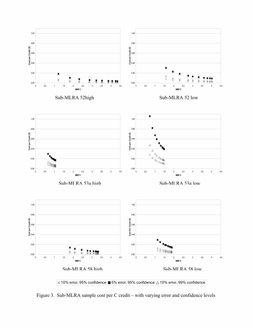
produced. Figure 3 plots the cost/credit of measuring and monitoring against the total number of

credits produced at payments between $10 to $100/credit in each agroecozone over three error

and confidence combinations. Measuring and monitoring costs range between a low of 1 cent per

C-credit in sub-MLRA 52-high to 28 cents per C-credit in sub-MLRA 53a-low assuming a 10%

error and 95% confidence interval, figure 3. In each sub-MLRA the measuring and monitoring

costs per credit exhibit economies of scale. As the number of C-credits produced in a region

increase the average measuring and monitoring cost per credit decreases. This is driven by two

factors. First, as the price per C-credit increases, the sample size decreases (table 3) and second

as the price per C-credit increases the number of C-credits produced also increases. A decrease in

acceptable error or an increase in the desired confidence level increase the costs of measurement

and monitoring in proportion with the sample size shown in table 3, i.e. if sample size increases

by 4, the measurement and monitoring cost per credit also increases by 4 at any given payment

level within an agroecozone. This result is driven by the fact that we have assumed that the cost

of an individual sample remains constant and independent of the sample size.

Tables 4a, b and c, show that as a percentage of the total credit price, measuring and

monitoring costs per credit range between 100th of 1% to 10.6%. At 10% error and 95%

confidence (consistent with several forestry projects) measurement costs do not exceed 3% of the

credit purchase price.

Spatial heterogeneity, sample size and measurement and monitoring costs

Both sample size and measurement and monitoring costs per C-credit vary between each

agroecozone at every price level, table 3 and figure 3. Regional differences in measuring and

monitoring costs can be explained in part by the different degrees of spatial heterogeneity in

rates of C sequestration exhibited by each area. The relative spatial heterogeneity of soil C

changes in an agroecozone is represented by the coefficient of variation. Table 5 reports the

sample size and spatial heterogeneity of an area. The data indicate that these two variables are

positively related. Figure 4a demonstrates that the measuring and monitoring cost per C-credit is

positively related to the degree of spatial heterogeneity within an area. At any given price,

regions with greatest spatial heterogeneity are associated with the largest samples and the

highest costs of measuring and monitoring per C-credit, supporting our earlier statement.

Figure 4a demonstrates that there are also other factors that influence the measuring and

monitoring costs per C-credit. For example, sub-MLRAs 52-high and 53a-low exhibit the same

spatial heterogeneity at several points but the measuring and monitoring costs per credit are

higher in sub-MLRA 52-high over this range. Figure 4b demonstrates that measuring and

monitoring costs per C-credit decline as the total number of credits produced within an area

increase. Figures 4a and 4b suggest that the measurement and monitoring cost per C-credit is in

part determined by the spatial heterogeneity of soil C rates within an area and the economic and

biophysical resource endowments that govern producer participation and C-credit generation at

each price level.

Conclusions

This paper develops a conceptual measurement and monitoring protocol for C-credits

generated by increasing agricultural soil C under per-tonne contracts. An empirical example of

this framework is implemented for the dry-land crop producing region of Montana and used to

examine the factors that influence measuring and monitoring costs for soil C. We hypothesize

that the sample size and measuring and monitoring costs per C-credit within a given region are

influenced by the market price for C-credits and the spatial heterogeneity of C-credit

accumulation. Results from the empirical application support these hypotheses and demonstrate

that the measuring and monitoring costs per C-credit are inversely related to the price offered for

each credit. In addition, at every price level for C-credits, the measuring and monitoring cost per

credit is larger in regions that exhibit higher spatial heterogeneity. A decrease in the acceptable

sampling error or an increase in the confidence level raise the costs of measuring and monitoring.

The proportional increase in costs is larger for a decrease in the acceptable error.

The results presented above have several implications for the costs of measuring and

monitoring soil C-credits and the relative efficiency of a per-tonne contract design versus a per-

hectare contract design. First, the measuring and monitoring costs per C-credit could be a very

small percentage of the value of the credit as reflected in the payment level. In this analysis the

measuring and monitoring costs ranged between a maximum of 3% to 10.6% of total credit value

(depending on the assumed error and confidence level). This suggests that in most cases the

additional costs of a measuring and monitoring protocol for C-credits is unlikely to make a per

tonne contract less efficient than the per hectare contract, unless the opportunity costs of

supplying C-credits are very similar under both contract schemes. Previous work by Antle et al.

(2002b) shows that the efficiency gain from a per-tonne contract over a per-hectare contract

increases with the degree of spatial heterogeneity, in each region and although measuring and

monitoring costs per C-credit are also positively related to spatial heterogeneity, they do not

outweigh the efficiency gains. Regions with high heterogeneity are able to support higher

measuring and monitoring costs as they have the greatest difference in the opportunity cost of

supplying C-credits under each contract type.

Second, the error and confidence level chosen for the sample design will be, in part, a

function of the value of each C-credit. At high credit prices there are larger costs to over or under

estimating the number of credits, thus more resources could be merited for measurement and

monitoring. Third, the measurement and monitoring costs are influenced by the size of each

contract region. Under the measuring and monitoring protocol, soil C accumulation rates are

fixed over each region and are independent of the actual location and composition of the

population supplying C-credits. When the population supplying C-credits is small (at low prices)

estimated measuring and monitoring costs per C-credit could be larger than necessary because

the variability of soil C rates could be overstated. This suggests that the optimal size of each

contract area could be related to the price offered for C-credits. The general results from this

study are likely to apply to other agricultural regions that are considering supplying C-credits and

implementing a measuring and monitoring scheme.

Extensions to the current work could provide additional insight into the optimal design of

measuring and monitoring schemes for soil C-credits. For example, alternative sampling

schemes could be considered as well as the implications of changing the spatial scale of analysis

on measuring and monitoring costs. In addition the question of adjusting estimated C-variability

to reflect the population at each price level merits further investigation.

Several other issues that could influence contracting costs are not considered in this

paper. In addition to C-sequestration, agricultural practices influence the emissions of other

greenhouse gases. Ideally, efforts to mitigate greenhouse gases would require a full accounting

framework that accounts for both changes in the net emissions of C (as discussed here) as well as

nitrous oxide and other gases. These gases will also require monitoring, and this could further

increase contracting costs. A second important issue not addressed in this paper relates to the

transactions costs associated with assembling a large number of producers to jointly fill C-

contracts.

References

Antle, J.M. and S. Mooney. 2002. “Designing Efficient Practices for Agricultural Soil Carbon

Sequestration.” In J.M. Kimble, R. Lal, and R.F. Follett, eds., Agriculture Practices and Policies for Carbon Sequestration in Soil, Boca Raton, FL: CRC Press LLC, pp. 323–336.

Antle, J.M., S.M. Capalbo, S. Mooney, E.T. Elliott, and K.H. Paustian. 2002a. “A Comparative

Examination of the Efficiency of Sequestering Carbon in U.S. Agricultural Soils.” American Journal of Alternative Agriculture 17(1), in press.

Antle, J.M., S.M. Capalbo, S. Mooney, E.T. Elliott, and K.H. Paustian. 2002b. “Spatial

Heterogeneity, Contract Design, and the Efficiency of Carbon Sequestration Policies for Agriculture.” Research Program on the Economics of Climate Change and Greenhouse Gas Mitigation at Montana State University–Bozeman. http://www.climate.montana.edu.

Antle, J.M., S.M. Capalbo, S. Mooney, E.T. Elliott, and K.H. Paustian. 2001a. “Economic

Analysis of Agricultural Soil Carbon Sequestration: An Integrated Assessment Approach.” Journal of Agricultural and Resource Economics 26(2):344–367.

Antle, J.M. and S.M. Capalbo. 2001b. “Econometric-Process Models for Integrated Assessment

of Agricultural Production Systems.” American Journal of Agricultural Economics 83(2):389–401.

Boscolo, M., M. Powell, M. Daleney, S. Brown, and R. Faris. 2000. “The Cost of Inventorying

and Monitoring Carbon: Lessons from the Noel Kempff Climate Action Project.” Journal of Forestry 98(9):24–31.

Brown, S. 1999. Guidelines for Inventorying and Monitoring Carbon Offsets in Forest Based

Projects, Winrock International.

Brown, S., M. Burnham, M. Delaney, M. Powell, R. Vaca, and A. Moreno. 2000. “Issues and Challenges for Forest-Based Carbon-Offset Projects: A Case Study of the Noel Kempff Climate Action Project in Bolivia.” Mitigation and Adaptation Strategies for Global Change 5(1):99–121.

Environmental News Network (ENN). 2001. Montana Tribes Make First Carbon Offset Trade.

Wednesday, April 4. http://www.enn.com/news/enn-stories/2001/04/04042001/ carbon_42869.asp

Lal, R., L.M. Kimble, R.F. Follett, and C.V. Cole. 1998. The Potential of U.S. Cropland to Sequester C and Mitigate the Greenhouse Effect. Chelsea, MI: Ann Arbor Press.

MacDicken, K.G. 1997. A Guide to Monitoring Carbon Storage in Forestry and Agroforestry

Projects. Winrock International Institute for Agricultural Development.

McConkey, B. and W. Lindwall. 1999. “Measuring Soil Carbon Stocks: A System for Quantifying and Verifying Change in Soil Carbon Stocks Due to Changes in Management Practices on Agricultural Land.” Agriculture and Agri-Food Canada.

McCall, C.H., Jr. 1982. Sampling and Statistics Handbook for Research. Ames, IA: The Iowa

State University Press. Mann, L.K. 1986. “Changes in Soil C Storage after Cultivation.” Soil Science 142(5):279–288. Moxey, A., B. White, and A. Ozanne. 1999. “Efficient Contract Design for Agri-Environment

Policy.” Journal of Agricultural Economics 50(2):187-202. PacifiCorp. 1997. PacifiCorp’s Commitment to the Environment: CO2 Initiatives. October.

Portland, Oregon. Parton, W.J., D.S. Schimel, D.S. Ojima, and C.V. Cole. 1994. “A General Model for Soil

Organic Matter Dynamics: Sensitivity to Litter Chemistry, Texture and Management.” In R.B. Bryant and R.W. Arnold, eds., Quantitative Modeling of Soil Forming Processes. SSSA Special Publication Number 39. Soil Science Society of America, Madison, WI, pp. 147–167.

Paustian, K., E.T. Elliott, and L. Hahn. 1999. “Agroecosystem Boundaries and C Dynamics with

Global Change in the Central United States.” FY 1998/1999 Progress Report, The National Institute for Global Environment Change (NIGEC). Available online at http://nigec.ucdavis.edu/publications/annual99/greatplains/GPPaustian0.html.

Paustian, K., E.T. Elliott, G.A. Peterson, and K. Killian. 1996. “Modelling Climate, Co2 and

Management Impacts on Soil Carbon in Semi-arid Agroecosystems.” Plant and Soil 187(2):351–365.

Pautsch, G.R., L.A. Kurkalova, B.A. Babcock, and C.L. Kling. 2001. “The Efficiency of

Sequestering Carbon in Agricultural Soils.” Contemporary Economic Policy 19(2)123–134.

Rasmussen, P.E. and W.J. Parton. 1994. “Long-term Effects of Residue Management in Wheat

Fallow: I. Inputs, Yield and Soil Organic Matter.” Soil Science Society of America Journal 58(2):523–530.

Rosenzweig, R., M. Varilek, B. Feldman, R. Kuppalli, and J. Janssen. 2002. “The Emerging

International Greenhouse Gas Market.” Pew Center for Global Climate Change. Sarndal, C., B. Swensson, and J. Wretman. 1992. Model Assisted Survey Sampling. Springer-

Verlag New York, Inc.

Smith, G.R. 2002. “Case Study of Cost versus Accuracy When Measuring Carbon Stock in a Terrestrial Ecosystem.” In J. Kimble, ed., Agriculture Practices and Policies for Carbon Sequestration in Soil. CRC Press LLC.

Stavins, R.N. 1998. “A Methodological Investigation of the Costs of Carbon Sequestration.” Journal of Applied Economics 1(2):231–277.

Stavins, R.N. 1999. “The Costs of Carbon Sequestration: A Revealed-Preference Approach.” American Economics Review 89(4):994–1009.

Thompson, S.K. 1992. Sampling. New York: John Wiley and Sons, Inc. Tiessen, H., J.W.B. Stewart, and J.R. Bettany. 1982. “Cultivation Effects on the Amounts and

Concentration of Carbon, Nitrogen and Phosphorous in Grassland Soils.” Agronomy Journal 74:831–835.

United Nations Framework Convention on Climate Change (UNFCCC). 1998. Reports of the

Conference of the Parties on its third session, held at Kyoto from 1 to 11 December 1997. FCCC/CP/1997/7/Add1. 18th March 1998.

United Nations Framework Convention on Climate Change (UNFCCC). 2002. Report of the

Conference of the Parties on its Seventh Session, held at Marrakech from 29 October to 10 November 2001. Addendum. Part two: Action Taken by the Conference of the Parties. Volume I. FCCC/CP/2001/13/Add.1.

Vine, E. and J. Sathaye. 1997. “The Monitoring, Evaluation, Reporting, and Verification of Climate Change Mitigation Projects: Discussion of Issues and Methodologies and Review of Existing Protocols and Guidelines.” Energy Analysis Program, Environmental Energy Technologies Division, Lawrence Berkeley National Laboratory, Berkeley, CA 94720.

Vine, E., J. Sathaye and W. Makundi. 1999. “The Monitoring, Evaluation, Reporting, Verification and Certification of Climate Change Forest Projects.” LBNL-41877. Lawrence Berkeley National Laboratory, Berkeley, CA.

Watson, R.T., M.C. Zinyowera, R. H. Moss, and D.J. Dokken, eds. 1996. Climate Change 1995:Impacts, Adaptations and Mitigation of Climate Change: Scientific-Technical Analysis. Contribution of Working Group II to the Second Assessment Report of the Intergovernmental Panel on Climate Change, World Meteorological Organization, and the United Nations Environment Programme, Cambridge, UK: Cambridge University Press.

Watson, R.T, I.R. Noble, B. Bolin, N.H. Ravindranath, D.J. Verardo, and D. J. Dokken. 2000.

“Land Use, Land-Use Change and Forestry.” A Special Report of the Intergovernmental Panel on Climate Change, Cambridge, UK: Cambridge University Press.

Whitby, M and C. Saunders. 1996. “Estimating the Supply Curve of Conservation Goods in Britain: A Comparison of the Financial Efficiency of Two Policy Instruments.” Land Economics 72:313-325.

White House. 2002. Global Climate Change Policy Book. http://www.whitehouse.gov/news/

releases/2002/02/climatechange.html (downloaded 2/15/01). Wu, J. and B.A. Babcock. 1996. “Contact Design for the Purchase of Environmental Goods from

Agriculture.” American Journal of Agricultural Economics 78(4):935–945.

Figure 1. Costs associated with negotiating contracts for soil carbon sequestration

Steps for exchange in C Associated costs

Identify eligible managementPractices and payment levels

Producers participating in scheme

Form contracts betweenbuyers and sellers

Measurement and monitoring

Identification costs

Negotiations/legal costs

Monitoring and compliance costs

Common to per-hectareand per-

tonnecontracts

Required under a per-

tonne contract only

Practices

Carbon

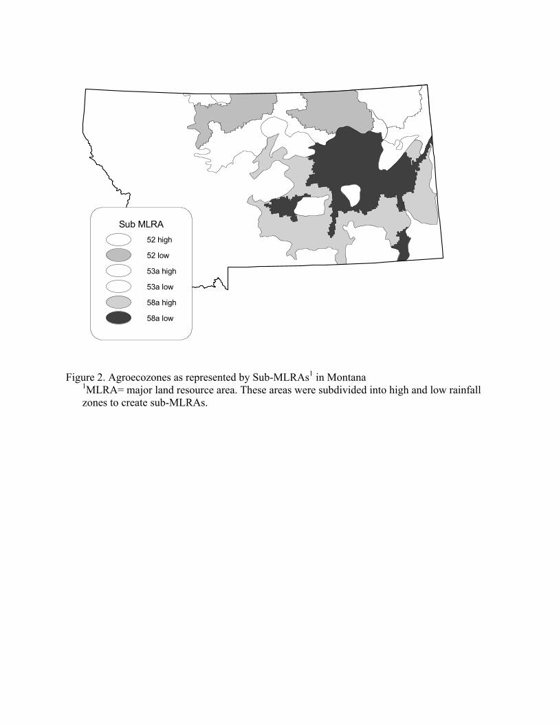
Figure 2. Agroecozones as represented by Sub-MLRAs1 in Montana 1MLRA= major land resource area. These areas were subdivided into high and low rainfall zones to create sub-MLRAs.

Sub MLRA52 high

52 low

53a high

53a low

58a high

58a low

0.00

0.05

0.10

0.15

0.20

0.25

0.30

0.35

0 0.5 1 1.5 2 2.5

MMT C

Cost

Per

Cre

dit (

$)

10% error, 95% confidence 5% error, 95% confidence 10% error, 99% confidence

0.00

0.20

0.40

0.60

0.80

1.00

0 0.5 1 1.5 2 2.5 3 3.5 4 4.5

MMT C

Cos

t per

Cre

dit (

$)

0.00

0.20

0.40

0.60

0.80

1.00

0 0.5 1 1.5 2 2.5 3 3.5 4 4.5

MMT C

Cos

t per

Cre

dit (

$)

0.00

0.20

0.40

0.60

0.80

1.00

0 0.5 1 1.5 2 2.5 3 3.5 4 4.5

MMT C

Cos

t per

Cre

dit (

$)

0.00

0.20

0.40

0.60

0.80

1.00

0 0.5 1 1.5 2 2.5 3 3.5 4 4.5

MMT C

Cos

t per

Cre

dit (

$)

0.00

0.20

0.40

0.60

0.80

1.00

0 0.5 1 1.5 2 2.5 3 3.5 4 4.5

MMT C

Cos

t per

Cre

dit (

$)

0.00

0.20

0.40

0.60

0.80

1.00

0 0.5 1 1.5 2 2.5 3 3.5 4 4.5

MMT C

Cos

t Per

Cre

dit (

$)

Sub-MLRA 52high Sub-MLRA 52 low

Sub-MLRA 53a high Sub-MLRA 53a low

Sub-MLRA 58 high Sub-MLRA 58 low

Figure 3. Sub-MLRA sample cost per C credit – with varying error and confidence levels

Figure 4a. Measurement and monitoring cost per credit and coefficient of variation in C.

Figure 4b. Measurement and monitoring cost per credit and total number of credits.

0.00

0.05

0.10

0.15

0.20

0.25

0.30

00.511.522.533.5

Coefficient of Variation

Cos

t/cre

dit

52H 52L 53H 53l 58H 58L

0.00

0.05

0.10

0.15

0.20

0.25

0.30

0.00 0.50 1.00 1.50 2.00 2.50 3.00 3.50 4.00 4.50 5.00

C-credits (MMT C)

Cos

t/cre

dit (

$)

52high 52low 53high 53low 58high 58low

Table 1. Data sources for sample size calculations at a given C credit price

Variable Name Value Source

Z 1.96 (95% confidence)

Normal tables

ε Varies by agroecozone

Product of relative error (0.1) and the weighted average of estimated strata means. Estimated mean C changes were obtained from CENTURY model runs.

N Varies by agroecozone

Number of hectares that enter into contracts to supply C credits at a given price within an agroecozone. Obtained from simulation model results.

j Varies by agroecozone

Number of strata within an agroecozone. Obtained from simulation model results.

Nj Varies by agroecozone and

stratum

Number of hectares within stratum j. Obtained from simulation model results.

jσ~ Varies by agroecozone and

stratum

Estimated standard deviation of C changes within each strata and agroecozone. Calculated from input data to Century model.

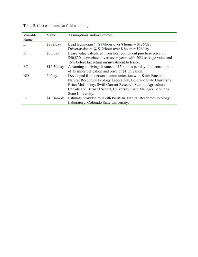
Table 2. Cost estimates for field sampling Variable Name

Value Assumptions and/or Sources

L $232/day Lead technician @ $17/hour over 8 hours = $136/day Driver/assistant @ $12/hour over 8 hours = $96/day

R $70/day Lease value calculated from total equipment purchase price of $40,830, depreciated over seven years with 20% salvage value and 15% before tax return on investment to lessor.

FC $16.50/day Assuming a driving distance of 150 miles per day, fuel consumption of 15 miles per gallon and price of $1.65/gallon.

ND 50/day Developed from personal communication with Keith Paustian, Natural Resources Ecology Laboratory, Colorado State University; Brian McConkey, Swift Current Research Station, Agriculture Canada and Bernard Schaff, University Farm Manager, Montana State University.

LC $10/sample Estimate provided by Keith Paustian, Natural Resources Ecology Laboratory, Colorado State University.

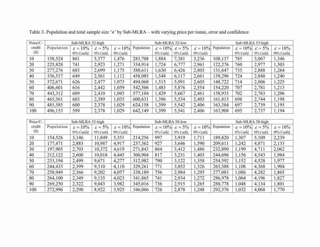
Table 3. Population and total sample size ‘n’ by Sub-MLRA – with varying price per tonne, error and confidence

Sub-MLRA 52-high Sub-MLRA 52-low Sub-MLRA 53-high Price/C-credit

($) Population %10=ε

95% Confid. %5=ε

95% Confid. %10=ε

99% Confid. Population %10=ε

95% Confid. %5=ε

95% Confid. %10=ε

99% Confid. Population %10=ε

95% Confid. %5=ε

95% Confid. %10=ε

99% Confid. 10 158,524 861 3,377 1,476 283,708 1,884 7,381 3,236 108,137 785 3,067 1,346 20 225,828 741 2,923 1,271 334,914 1,724 6,777 2,961 122,276 760 2,977 1,303 30 277,276 683 2,699 1,175 388,611 1,630 6,426 2,803 131,647 735 2,888 1,264 40 336,517 649 2,561 1,112 458,085 1,548 6,117 2,661 139,296 724 2,840 1,240 50 372,671 626 2,477 1,073 494,068 1,515 5,991 2,605 148,722 714 2,806 1,225 60 406,601 616 2,442 1,059 542,506 1,483 5,876 2,554 154,220 707 2,781 1,213 70 443,312 609 2,410 1,043 577,104 1,429 5,667 2,461 158,933 702 2,763 1,206 80 465,561 603 2,389 1,035 600,631 1,396 5,534 2,403 161,813 698 2,744 1,198 90 485,585 600 2,378 1,029 624,158 1,399 5,542 2,406 163,384 697 2,739 1,195 100 496,153 599 2,378 1,029 642,149 1,399 5,541 2,406 163,908 695 2,737 1,194

Sub-MLRA 53-high Sub-MLRA 58-low Sub-MLRA 58-high Price/C-credit

($) Population %10=ε

95% Confid. %5=ε

95% Confid. %10=ε

99% Confid. Population %10=ε

95% Confid. %5=ε

95% Confid. %10=ε

99% Confid. Population %10=ε

95% Confid. %5=ε

95% Confid. %10=ε

99% Confid. 10 154,526 3,146 11,849 5,351 214,256 997 3,919 1,711 189,820 1,307 5,109 2,239 20 177,471 2,883 10,987 4,917 237,362 927 3,646 1,590 209,611 1,242 4,871 2,133 30 197,905 2,703 10,372 4,619 271,843 864 3,412 1,486 232,890 1,199 4,711 2,062 40 212,122 2,600 10,018 4,445 300,904 817 3,231 1,403 244,696 1,156 4,543 1,984 50 233,194 2,499 9,671 4,277 312,982 790 3,122 1,358 254,592 1,152 4,528 1,977 60 244,433 2,399 9,310 4,110 329,261 771 3,052 1,326 265,388 1,108 4,368 1,904 70 258,949 2,366 9,202 4,057 338,189 756 2,984 1,295 277,083 1,086 4,282 1,865 80 264,100 2,349 9,135 4,023 341,865 741 2,934 1,272 286,978 1,064 4,196 1,827 90 269,250 2,322 9,043 3,982 345,016 736 2,915 1,265 288,778 1,048 4,134 1,801 100 272,996 2,290 8,922 3,925 346,066 726 2,878 1,248 292,376 1,032 4,068 1,770

Table 4a. Estimated cost of measurement and monitoring per credit – 10% error, 95% confidence

Sub-MLRA 52-high Sub-MLRA 52-low Sub-MLRA 53-high Sub-MLRA 53-low Sub-MLRA 58-high Sub-MLRA 58-low Price/credit ($)

MPQ ($)

Measurement Cost

(% of Price)

MPQ ($)

Measurement Cost

(% of Price)

MPQ ($)

Measurement Cost

(% of Price)

MPQ ($)

Measurement Cost

(% of Price)

MPQ ($)

Measurement Cost

(% of Price)

MPQ ($)

Measurement Cost

(% of Price) 10 0.046 0.463 0.077 0.774 0.077 0.765 0.281 2.808 0.036 0.356 0.075 0.749 20 0.027 0.133 0.058 0.289 0.065 0.323 0.215 1.076 0.029 0.145 0.063 0.316 30 0.019 0.064 0.046 0.154 0.057 0.190 0.175 0.584 0.023 0.077 0.054 0.181 40 0.015 0.037 0.037 0.091 0.053 0.132 0.155 0.386 0.019 0.048 0.049 0.122 50 0.013 0.025 0.033 0.066 0.049 0.097 0.133 0.266 0.018 0.036 0.047 0.094 60 0.011 0.019 0.029 0.049 0.046 0.077 0.119 0.199 0.016 0.027 0.043 0.071 70 0.010 0.015 0.026 0.037 0.045 0.064 0.111 0.158 0.015 0.022 0.040 0.057 80 0.010 0.012 0.024 0.030 0.043 0.054 0.107 0.134 0.015 0.019 0.038 0.047 90 0.009 0.010 0.023 0.026 0.043 0.048 0.104 0.115 0.015 0.016 0.037 0.041 100 0.009 0.009 0.023 0.023 0.043 0.043 0.100 0.100 0.014 0.014 0.035 0.035 Table 4b. Estimated cost of measurement and monitoring per credit – 5% error, 95% confidence

Sub-MLRA 52-high Sub-MLRA 52-low Sub-MLRA 53-high Sub-MLRA 53-low Sub-MLRA 58-high Sub-MLRA 58-low Price/credit ($)

MPQ ($)

Measurement Cost

(% of Price)

MPQ ($)

Measurement Cost

(% of Price)

MPQ ($)

Measurement Cost

(% of Price)

MPQ ($)

Measurement Cost

(% of Price)

MPQ ($)

Measurement Cost

(% of Price)

MPQ ($)

Measurement Cost

(% of Price) 10 0.181 1.815 0.303 3.031 0.299 2.990 1.057 10.574 0.140 1.399 0.293 2.927 20 0.105 0.523 0.227 1.125 0.253 1.265 0.820 4.102 0.114 0.570 0.248 1.238 30 0.076 0.254 0.182 0.606 0.224 0.748 0.672 2.241 0.091 0.304 0.213 0.709 40 0.058 0.146 0.145 0.362 0.207 0.518 0.596 1.489 0.077 0.192 0.192 0.481 50 0.050 0.101 0.131 0.261 0.192 0.383 0.515 1.030 0.070 0.141 0.185 0.370 60 0.045 0.075 0.116 0.193 0.183 0.304 0.464 0.773 0.065 0.108 0.169 0.281 70 0.041 0.058 0.103 0.147 0.176 0.251 0.431 0.615 0.061 0.087 0.158 0.226 80 0.038 0.048 0.096 0.120 0.171 0.214 0.418 0.522 0.059 0.074 0.148 0.186 90 0.037 0.041 0.096 0.103 0.169 0.188 0.404 0.449 0.058 0.064 0.144 0.161 100 0.036 0.036 0.090 0.090 0.168 0.168 0.391 0.391 0.057 0.057 0.139 0.139 MPQ=measurement and monitoring cost per tonne C.

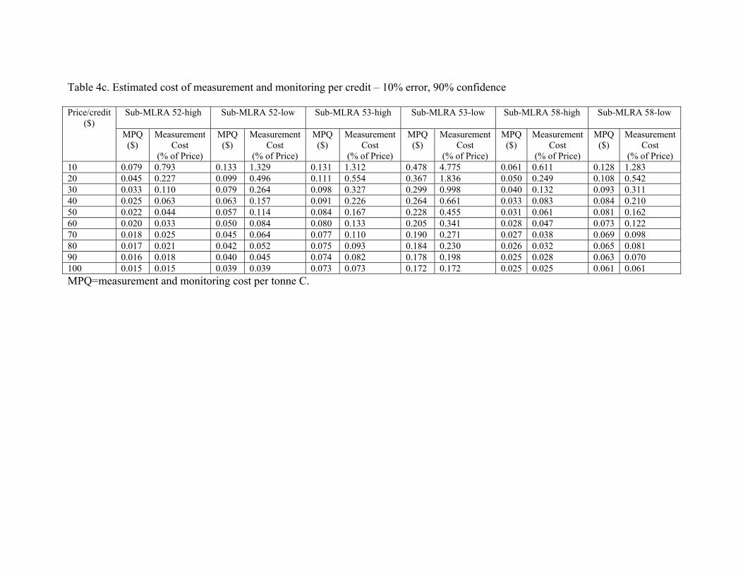
Table 4c. Estimated cost of measurement and monitoring per credit – 10% error, 90% confidence

Sub-MLRA 52-high Sub-MLRA 52-low Sub-MLRA 53-high Sub-MLRA 53-low Sub-MLRA 58-high Sub-MLRA 58-low Price/credit ($)

MPQ ($)

Measurement Cost

(% of Price)

MPQ ($)

Measurement Cost

(% of Price)

MPQ ($)

Measurement Cost

(% of Price)

MPQ ($)

Measurement Cost

(% of Price)

MPQ ($)

Measurement Cost

(% of Price)

MPQ ($)

Measurement Cost

(% of Price) 10 0.079 0.793 0.133 1.329 0.131 1.312 0.478 4.775 0.061 0.611 0.128 1.283 20 0.045 0.227 0.099 0.496 0.111 0.554 0.367 1.836 0.050 0.249 0.108 0.542 30 0.033 0.110 0.079 0.264 0.098 0.327 0.299 0.998 0.040 0.132 0.093 0.311 40 0.025 0.063 0.063 0.157 0.091 0.226 0.264 0.661 0.033 0.083 0.084 0.210 50 0.022 0.044 0.057 0.114 0.084 0.167 0.228 0.455 0.031 0.061 0.081 0.162 60 0.020 0.033 0.050 0.084 0.080 0.133 0.205 0.341 0.028 0.047 0.073 0.122 70 0.018 0.025 0.045 0.064 0.077 0.110 0.190 0.271 0.027 0.038 0.069 0.098 80 0.017 0.021 0.042 0.052 0.075 0.093 0.184 0.230 0.026 0.032 0.065 0.081 90 0.016 0.018 0.040 0.045 0.074 0.082 0.178 0.198 0.025 0.028 0.063 0.070 100 0.015 0.015 0.039 0.039 0.073 0.073 0.172 0.172 0.025 0.025 0.061 0.061 MPQ=measurement and monitoring cost per tonne C.

Table 5. Coefficient of variation in C and sample size (10% error, 95% confidence)

Sub-MLRA 52-high Sub-MLRA 52-low Sub-MLRA 53-high Sub-MLRA 53-low Sub-MLRA 58-high Sub-MLRA 58-low Price/credit ($) CV Sample

Size CV Sample

Size CV Sample

Size CV Sample

Size CV Sample

Size CV Sample

Size 10 1.49 861 2.22 1,884 1.43 785 2.89 3,146 1.61 997 1.84 1,307 20 1.38 741 2.12 1,724 1.40 760 2.76 2,883 1.55 927 1.80 1,242 30 1.33 683 2.06 1,630 1.38 735 2.66 2,703 1.49 864 1.76 1,199 40 1.29 649 2.00 1,548 1.37 724 2.61 2,600 1.45 817 1.73 1,156 50 1.27 626 1.98 1,515 1.36 714 2.56 2,499 1.43 790 1.73 1,152 60 1.26 616 1.96 1,483 1.35 707 2.50 2,399 1.41 771 1.70 1,108 70 1.25 609 1.92 1,429 1.35 702 2.49 2,366 1.40 756 1.68 1,086 80 1.25 603 1.90 1,396 1.34 698 2.48 2,349 1.38 741 1.66 1,064 90 1.24 600 1.90 1,399 1.34 697 2.46 2,322 1.38 736 1.65 1,048 100 1.24 599 1.90 1,399 1.34 695 2.45 2,290 1.37 726 1.63 1,032