Embed Size (px)
Citation preview

Contribution to Laboratorial Determination of Rheological
Properties of Paste Backfill
Zinkgruvan and Neves-Corvo Case Studies
Maria Ângela Marques do Carmo Silva
Dissertation to obtain the Master of Science Degree in
Geological and Mining Engineering
Supervisor: Prof. Dr. Maria Matilde Mourão de Oliveira Carvalho Horta Costa e Silva
Examination Committee
Chairperson: Prof. Dr. Maria Teresa da Cruz Carvalho
Supervisor: Prof. Dr. Maria Matilde Mourão de Oliveira Carvalho Horta Costa e Silva
Members of the Committee: Eng. Hugo Miguel Costa Brás
May 2017


i
The present dissertation is dedicated to my parents…

ii

iii
“Simplicity is the highest goal achievable when you have overcome all difficulties”
Frederic Chopin

iv

v
ABSTRACT
Rheology is among the most important properties of paste backfill that determine its transportability for long
distances underground. The rheological characterisation of paste backfill is a difficult and complex task, given
the high number of variable factors. So far, no standard procedures and/or methods have been established for
measuring the rheological properties of paste backfill, in particular the yield stress.
The experimental work carried out here consisted of the development of an accurate laboratorial testing
programme that would allow the evaluation, measurement and understanding of the rheological properties of
this type of material. To this end, an extensive battery of laboratorial tests was conducted at the GeoLab, Instituto
Superior Técnico, on different paste fill mixtures produced with cement, tap water and tailings from the
Zinkgruvan and Neves-Corvo mines.
To determine the viscosity and yield stress of these mixtures, the following test methods were carried out:
slump, flow table (for cement mortar), fall cone and the vane technique (applied using a viscometer and a
rheometer). From the results achieved, the test methods that achieved the best results and correlations with the
dry content of the mixtures and with the values of yield stress measured by the viscometer and rheometer were
identified. Some conclusions drawn about the impact of parameters of yield stress values, determined by both
pieces of equipment, were mathematically proven in a statistical study based on the proposal and validation of
multiple linear regression models.
The fall cone test, adapted to this type of material, showed the best results/performance and thus plays a
major role in this dissertation. Being a simple, inexpensive and expedited method for paste yield stress
measurement, it is considered to be ideal for quality control and/or rapid on-site measurements of paste fill.
Keywords
Paste backfill; rheology; yield stress; viscosity; mine backfill; Zinkgruvan; Neves-Corvo

vi

vii
RESUMO
A reologia é uma das propriedades mais importantes do enchimento de pasta, na medida em que determina
a viabilidade de transporte deste material por longas distâncias no subsolo. A caracterização reológica da pasta
de enchimento constitui uma tarefa difícil, complexa, ainda assim, desafiante, tendo em conta o elevado número
de fatores variáveis. Até ao momento, ainda não foram criados procedimentos e/ou métodos standard para a
medição das propriedades reológicas deste material, de forma particular, a tensão de cedência.
O trabalho experimental realizado consistiu no desenvolvimento de um programa preciso de testes
laboratoriais que permitisse avaliar, medir e compreender as propriedades reológicas deste tipo de pasta. Neste
sentido, realizou-se uma vasta bateria de ensaios, no laboratório GeoLab, no Instituto Superior Técnico, a
diferentes misturas, produzidas com cimento, água e rejeitados provenientes das minas de Zinkgruvan e de
Neves-Corvo.
Para determinar a viscosidade e a tensão de cedência destas misturas, efetuaram-se os ensaios seguintes:
slump (abaixamento), flow table (mesa de espalhamento), fall cone (cone de queda) e vane (aplicada através de
um viscosímetro e de um reómetro). A partir dos resultados obtidos, procedeu-se à identificação dos ensaios
que apresentaram melhores resultados e correlações com o teor de sólidos das misturas e com os valores de
tensão de cedência obtidos com o viscosímetro e com o reómetro. As conclusões obtidas sobre a influência de
certos parâmetros nos valores de tensão de cedência, determinados por ambos os equipamentos, foram
matematicamente comprovadas num estudo estatístico baseado na proposta e validação de modelos de
regressão linear múltipla.
O método de ensaio fall cone, adaptado a este tipo de material, foi o que obteve melhores resultados.
Tratando-se de um método simples, económico e expedito para a determinação da tensão de cedência de pasta,
considera-se que o estudo realizado constitui um importante contributo para a medição da tensão de cedência,
pelo que se recomenda a sua frequente utilização no controlo de qualidade e nas medições, in situ, deste tipo
de enchimento mineiro.
Palavras-chave
Enchimento de pasta; reologia; tensão de cedência; viscosidade; enchimento mineiro; Zinkgruvan; Neves-Corvo

viii

ix
ACKNOWLEDGEMENTS
Firstly, this work would not be possible without the support of the Sika Corporation, in particular Sika
Portugal. Therefore, I would like to express my sincere gratitude to Eng. Martin Hansson for giving me the
opportunity to develop my dissertation on this theme with Sika support and, especially, for his interest in my
work. It was a real privilege to know and work by the side of such a skilled professional.
I also would like to thank Rute Silva and Tiago Silva, who provided equipment, material and the means to do
the experimental work and to express my gratitude for the guidance and assistance given by the Sika R&D
department, through Dr. Christoff Kurz and Fabian Erismann.
For my academic activities, I am grateful to the Instituto Superior Técnico for its dedication to excellence and
quality education. In particular, I would like to express my sincere gratitude to my supervisor, Professor Matilde
Costa e Silva, for her advice and guidance on the experimental work and for her scientific and technical support
for the writing of this dissertation. I am also grateful to the engineer Gustavo Paneiro for his availability and help
with the data modelling for this work.
Thank you to all my professors on the Mining Engineering Master’s degree, in particular Professor Pedro
Bernardo for all his support to the students not only in terms of the technical and practical knowledge that he
imparted to us, but essentially for the opportunities that he set up within the mining industry.
I also owe a debt of gratitude to Somincor, in particular the engineer David Nicholls, for their continuous
support and openness to university students, allowing research projects and assisting them with their profound
experience and knowledge.
My profound gratitude goes to engineers Rodolfo Machado and Hugo Brás for their willingness and
confidence every time I needed their support. Thanks so much for everything!
I am also grateful to Faustino Oliveira for his availability and guidance on the experimental work.
I would also like to acknowledge my colleagues and friends, Raquel López, Rui Semeano, Paula Dias and Rafael
Caetano for their faithful companion on the good and bad times.
To Pedro Lino, a special acknowledgement for his loyalty, love and constant support.
Finally, I must express my profound gratitude to my parents and grandparents for providing me with unfailing
support and continuous encouragement throughout my years of study. Your unconditional love, support and
motivation are indispensable to me as I reach new stages in my life.

x

xi
TABLE OF CONTENTS
Abstract V
Resumo VII
Acknowledgements IX
Table of Contents X
List of Figures XIII
List of Tables XV
CHAPTER 1. INTRODUCTION
1.1 Motivation 1
1.2 Overview of the work 2
1.3 Thesis outline 3
CHAPTER 2. STATE OF THE ART
2.1 Mine backfill 4
2.2 Paste backfill 5
2.2.1 Supply of materials 5
2.2.2 Mix design 6
2.2.3 Production 9
2.2.4 Future challenges 10
2.3 Rheology 12
2.3.1 Rheological properties, concepts and models 12
2.4 Paste backfill rheology 18
2.4.1 Determinant factors 19
2.4.2 Yield Stress 21
2.4.3 Measurement methodologies 24
2.4.3.1 Indirect methods 24
2.4.3.2 Direct methods 25
2.4.3.2.1 Slump 25
2.4.3.2.2 Flow table 26
2.4.3.2.3 Inclined plane test 26
2.4.3.2.4 Cylindrical penetrometer 26
2.4.3.2.5 Fall cone instrument 27
2.4.3.2.6 Rheometry/Viscometry 27
2.4.3.2.7 Vane-shear instrument and technique 28
CHAPTER 3. EXPERIMENTAL WORK

xii
3.1 Mine tailings 30
3.1.1 Zinkgruvan Mine, Sweden 30
3.1.2 Neves-Corvo Mine, Portugal 31
3.1.3 Physical and chemical characterization of mine tailings 33
3.1.3.1 Particle size distribution 33
3.1.3.2 Chemical composition 35
3.1.3.3 Mineralogy 36
3.2 Testing design 37
3.2.1 Specimen preparation 37
3.2.2 Mixing 39
3.2.2.1 Mix design 39
3.2.2.2 Procedure 40
3.2.3 Test methods and procedures 40
3.2.3.1 Bulk density 40
3.2.3.2 Dry content 40
3.2.3.3 Slump 41
3.2.3.4 Flow table 42
3.2.3.5 Vane method 42
3.2.3.5.1 Viscometer 42
3.2.3.5.2 Rheometer 43
3.2.3.6 Fall cone 44
CHAPTER 4. RESULTS AND DATA ANALYSIS
4.1 Vane Method 46
4.1.1 DV1 Brookfield viscometer 46
4.1.2 Anton Paar rheometer 49
4.2 Slump 52
4.3 Flow table 56
4.4 Fall cone 60
4.5 Data analysis 64
4.6 Data modelling 68
CHAPTER 5. CONCLUSION AND RECOMMENDATIONS
5.1 Conclusion 75
5.2 Recommendations 77
References 79
Annexes
Annex I – Final laboratorial results – Zinkgruvan mixtures A1
Annex II - Final laboratorial results – Neves-Corvo mixtures A2

xiii
LIST OF FIGURES
CHAPTER 1. INTRODUCTION
Figure 1.1: Use of paste backfill technology worldwide (data from Yumlu, 2010) 1
CHAPTER 2. STATE OF THE ART
Figure 2.1: Schematic diagram showing the paste backfill mix variables: (1) mix ingredients, (2) transport
properties - flowability, (3) mechanical properties – stability (Belem and Benzaazoua, 2008) 7
Figure 2.2: Disc filters at the Neves-Corvo paste plant (14/09/2015) 9
Figure 2.3: Charging hopper at Zinkgruvan paste plant (21/12/2016) 10
Figure 2.4: Canadian backfill failures (De Souza et al, 2003) 11
Figure 2.5: Flow regimes in laminar flow (Paterson, 2011) 12
Figure 2.6: Viscosity model by Isaac Newton (Brookfield) 13
Figure 2.7: Newtonian fluid behaviour (Brookfield) 14
Figure 2.8: Shear thinning fluid behaviour (Brookfield) 14
Figure 2.9: Shear thickening fluid behaviour (Brookfield) 15
Figure 2.10: Plastic fluid behaviour (Brookfield) 15
Figure 2.11: Thixotropic fluid behaviour (Brookfield) 15
Figure 2.12: Shear stress versus shear rate curves for time-independent non-Newtonian slurries (He et al,
2004) 17
Figure 2.13: Canadian hard rock mine tailings particle size distribution curves envelop, adapted from Godbout,
2005 (Belem and Benzaazoua, 2008) 20
Figure 2.14: Typical flow curves. (a) Newonian; (b) Bingham (yield-constant plastic viscosity); (c) yield-
pseudoplastic (shear thinning); (d) yield dilatant (shear thickening) 21
Figure 2.15: Different yield stress values during shearing (Moller et al, 2006) 23
Figure 2.16: Slump test carried out at the Neves-Corvo and Zinkgruvan paste plants on 14/09/2015 and
21/12/2016 respectively 26
CHAPTER 3. EXPERIMENTAL WORK
Figure 3.1: Cumulative and density distributions of the 4 barrels of Neves-Corvo tailings 33
Figure 3.2: Cumulative and density distributions of the 4 barrels of Zinkgruvan tailings 34
Figure 3.3: SEM images of sample S1, Z1 and Z3 (left to right) 35
Figure 3.4: EDS spectra comparison of the samples S1 (black), Z1 (red) and Z3 (green) 35
Figure 3.5: Tailings homogenisation 37
Figure 3.6: Tailings separated in 11 bags from Zinkgruvan Mine (barrel 2) 37
Figure 3.7: Tailings of 4 barrels separated in 44 bags from Neves-Corvo Mine 38
Figure 3.8: Tailings weighing and drying oven 38
Figure 3.9: Samples of Zinkgruvan barrel 3 ready to mix, after water content measurement 38
Figure 3.10: Schematic diagram of barrels/mixtures distribution 39

xiv
Figure 3.11: Desiccator with a sample inside to cool to room temperature 41
Figure 3.12: Slump test 41
Figure 3.13: Flow table test 42
Figure 3.14: DV1 Brookfield rotational viscometer and vane spindles 43
Figure 3.15: Wingather SQ software 43
Figure 3.16: Anton Paar RheolabQC instrument, paste sample inside the container and vane spindle (from left to
right) 44
Figure 3.17: Fall cone instrument and standard steel cone 44
Figure 3.18: Formlabs 3D printer, on the left, and the cones printed with 600 and 300 degrees, on the right 45
Figure 3.19: Printed cones, positioned on the fall cone instrument 45
CHAPTER 4. RESULTS AND DATA ANALYSIS
Figure 4.1: Shear stress-time curves of Zinkgruvan paste fill mixtures as recorded by the viscometer 47
Figure 4.2: Shear stress-time curves for Neves-Corvo paste fill mixtures as recorded by the viscometer 48
Figure 4.3: Correlation graph of yield stress (measured by the viscometer) versus dry content of mixtures 48
Figure 4.4: Shear stress-time curves for Zinkgruvan paste fill mixtures as recorded by the rheometer 50
Figure 4.5: Shear stress-time curves for Neves-Corvo paste fill mixtures as recorded by the rheometer 50
Figure 4.6: Correlation graph of yield stress (measured by the rheometer) versus dry content of mixtures 51
Figure 4.7: Rheometer vane spindle and container 52
Figure 4.8: Photographic record of slump tests 53
Figure 4.9: Correlation graph of dry content of mixtures versus slump 53
Figure 4.10: Initial and final state of the material shape and stress distributions in a conical slump model (Schowalter
and Christensen 1998 and Clayton et al, 2003) where s/H is the dimensionless slump height, h0/H is the
dimensionless height of the undeformed region, h1/H is the dimensionless height of the deformed
region, dz is the thickness of the yielded section and rz the radius of the yielded section
54
Figure 4.11: Correlation graph of yield stress (measured by the viscometer) versus slump 54
Figure 4.12: Correlation graph of yield stress (measured by the rheometer) versus slump 55
Figure 4.13: Photographic record of flow table tests 56
Figure 4.14: Correlation graph of dry content of mixtures versus initial diameter of flow table tests 57
Figure 4.15: Correlation graph of yield stress (measured by the viscometer) versus initial diameter of flow table tests 57
Figure 4.16: Correlation graph of yield stress (measured by the rheometer) versus initial diameter of flow table tests 58
Figure 4.17: Correlation graph of dry content of mixtures versus final diameter of flow table tests 58
Figure 4.18: Correlation graph for yield stress (measured by the viscometer) versus final diameter of flow table tests 59
Figure 4.19: Correlation graph of yield stress (measured by the rheometer) versus final diameter of flow table tests 59
Figure 4.20: Photographic record of 300 and 600 fall cone tests 61
Figure 4.21: Correlation graph of dry content of mixtures versus penetration depth of 300 fall cone 61
Figure 4.22: Correlation graph for yield stress (measured by the viscometer) versus penetration depth of 300 fall
cone 62
Figure 4.23: Correlation graph of yield stress (measured by the rheometer) versus penetration depth of 300 fall cone 62
Figure 4.24: Correlation graph for dry content of mixtures versus penetration depth of 600 fall cone 63

xv
Figure 4.25: Correlation graph for yield stress (measured by the viscometer) versus penetration depth of 600 fall
cone 63
Figure 4.26: Correlation graph of yield stress (measured by the rheometer) versus penetration depth of 600 fall cone 64
Figure 4.27: Overlaying of the PSD curves of Zinkgruvan (orange) and Neves-Corvo tailings (yellow) on the Canadian
hard rock mine tailings PSD curves envelope 65
Figure 4.28: Studentized residuals histograms of models 3 and 7 70
Figure 4.29: Predicted versus observed values of yield stress (viscometer) using the best multiple linear model 71
Figure 4.30: Studentized residuals histograms of models 3 and 7 72
Figure 4.31: Predicted versus observed values of Yield stress (rheometer) using the best multiple linear model 73
LIST OF TABLES
CHAPTER 2. STATE OF THE ART
Table 2.1: Rheological parameters of different types of non-Newtonian fluids 17
Table 2.2: Practical applications of rheological properties 18
Table 2.3: Tailings classification system by Golder Paste Technology 19
Table 2.4: Details of experimental materials and techniques used in the inter-laboratory study 22
CHAPTER 3. EXPERIMENTAL WORK
Table 3.1: Mineral reserves – June 30, 2016 for Zinkgruvan Mine (http://www.lundinmining.com/s/Zinkgruvan.asp) 31
Table 3.2: Mineral resources (inclusive of mineral reserves) – June 30 2016 for Zinkgruvan Mine
(http://www.lundinmining.com/s/Zinkgruvan.asp) 31
Table 3.3: Expected production for Zinkgruvan Mine (http://www.lundinmining.com/s/Zinkgruvan.asp) 31
Table 3.4: Mineral reserves – June 30 2016 for Neves-Corvo Mine (http://www.lundinmining.com/s/Neves-Corvo.asp) 32
Table 3.5: Mineral resources (inclusive of mineral reserves) – June 30 2016 for Neves-Corvo Mine
(http://www.lundinmining.com/s/Neves-Corvo.asp) 32
Table 3.6: Expected production for Neves-Corvo Mine (http://www.lundinmining.com/s/Neves-Corvo.asp) 33
Table 3.7: The size distribution characteristics of Somincor and Zinkgruvan tailings 34
Table 3.8: Semi-quantitative evaluation of the element content (expressed as oxide) in S1, Z1 and Z3 samples 36
Table 3.9: Sieve fraction of sample S1, Z1 and Z3 36
Table 3.10: Quantitative phase analysis (Rietveld) of sieved tailings (< 63 μm) 36
CHAPTER 4. RESULTS AND DATA ANALYSIS
Table 4.1: Yield stress and viscosity values of Zinkgruvan and Neves-Corvo paste mixtures 47
Table 4.2: Yield stress and viscosity values of Zinkgruvan and Neves-Corvo paste mixtures 49
Table 4.3: Slump values of Zinkgruvan and Neves-Corvo paste mixtures 52
Table 4.4: Flow table values of Zinkgruvan and Neves-Corvo paste mixtures 56
Table 4.5: Fall cone values for Zinkgruvan and Neves-Corvo paste mixtures 60

xvi
Table 4.6: Coefficient of determination values of test methods versus the dry content of mixtures and the yield stress
values measured by viscometer and rheometer equipment (orange – Zinkgruvan mixtures; green – Neves-
Corvo mixtures)
67
Table 4.7: Multiple linear regression models considered in the study 69
Table 4.8: The analysis of variance (ANOVA) results of models 3 and 7 70
Table 4.9: AIC and SBIC of models 3 and 7 70
Table 4.10: Statistical significance analysis of the estimated parameters of regression model 3 71
Table 4.11: The analysis of variance (ANOVA) results of models 3 and 7 72
Table 4.12: AIC and SBIC of models 3 and 7 72
Table 4.13: Statistical significance analysis of the estimated parameters of regression model 3 73

1
CHAPTER 1. INTRODUCTION
1.1 Motivation
The mining industry is one of the largest producers of waste material in the world, creating (for example)
large volumes of sulphide-rich tailings during mineral processing operations. The disposal, stability and safety of
tailings and their effects on water and soil are important technical and environmental problems (Ercikdi et al,
2017). These materials are usually sent, as low-concentration slurries, to a waste disposal site or a tailings storage
facility (TSF), such as dams (Boger, 2006). When placed on surfaces, these structures are subject to some risks of
failure as a result of leakage, instability, liquefaction, erosion and poor design (Yilmaz and Fall, 2017). The
consequence of a dam failure is dramatic and can be tragic, leading to loss of human life, massive environmental
impacts and large monetary costs involved in compensation claims and clean-ups. (Boger, 2009) A total of 198
tailings dam accidents took place prior to 2000, and 22 after 2000 worldwide (Azam and Li 2010; WISE 2016).
As environmental pressure increases and intelligent water usage becomes crucial, the effective, economic
and environmental management of tailings has become a major issue for all mining operations around the world
(Yilmaz and Fall, 2017). As such, new technically suitable, economically viable, environmentally sustainable, and
socially responsible technologies have been created based on high concentration waste suspensions (Yilmaz and
Fall 2017). Paste backfill is one of the most important creations of the last 30 years that significantly reduces
surface tailings disposal by placing them safely in underground stopes, reducing environmental risks and post-
mining rehabilitation costs. (Yilmaz and Fall, 2017).
Aside from providing a safe way of storing tailings in underground mined-out voids, paste backfill also has
important advantages for ground stabilisation, such as: providing a safer work environment for miners and
allowing the exploitation of the adjacent stopes (increasing ore recovery) compared to common techniques such
as hydraulic and rock backfill. During recent years, many pioneer projects have proved the viability of paste
backfill systems and identified the challenges that need to be overcome for their implementation. A growing
number of underground mines are adopting paste backfill technology throughout Europe, Asia and South
America. In Australia and Canada, this type of backfilling is already applied in most mining projects (Figure 1.1).
Figure 1.1: Use of paste backfill technology worldwide (data from Yumlu, 2010)

2
Although major improvements have been achieved since its first application, key advances should be made
to further improve mining sustainability. The major challenges associated with this new technology relate to
efficient pumping/delivery of freshly mixed paste with high densities from the paste plant to the underground
cavities. Consequently, the transportability of the paste backfill is a crucial parameter in paste design. The
increased adoption of paste tailings has been facilitated by the improved ability to produce and handle paste
systems with a high concentration of solids (Sofra, 2017). Technological advancements in thickening, filtration,
centrifugation, mixing and pumping ability are all dependent on an increased understanding of paste flow
behaviour (rheology) and strength characteristics. A comprehensive understanding of the rheological
characteristics of cemented paste tailings throughout the paste operation is a prerequisite for achieving
successful paste surface deposition, and/or the desired characteristics for paste backfill (Sofra, 2017).
The rheological characterisation of fresh paste fill is a very complex and challenging task that requires the
gathering of useful data for paste operation design, due to its large number of variables. So far, no standard
procedures and/or methods have been established for measuring the rheological properties of paste backfill. As
a common practice, readily available techniques are used type of measurement.
This is the context of the present work: the necessity of accurate rheological testing programs to achieve
meaningful and valid results, along with the necessity of finding new approaches to measure rheological
properties and to understand the impact of the physical and chemical properties of tailings on the behaviour of
paste backfill.
1.2 Overview of the work
The experimental work conducted in this dissertation is focussed on the development of an accurate
laboratorial testing program to evaluate, measure and understand the rheological behaviour and properties of
fresh paste backfill. For that, a battery of experimental tests was conducted at the GeoLab at the Instituto
Superior Técnico in Lisbon, using different paste fill mixtures produced with cement, tap water and tailings from
Zinkgruvan and Neves-Corvo mines.
To this end, a physical and chemical characterisation of the tailings was carried out to understand their
differences and similarities in terms of granulometry and mineralogy. Different mix designs have been set for
each mine’s tailings, with a fixed percentage of cement of 4% to be tested in the laboratory. Each mixture was
characterised by its dry content and bulk density. Different test methodologies were used to evaluate the
rheological properties (viscosity and yield stress) of these mixtures, such as: the slump test, the flow table test
(for cement mortar) and the vane method using a viscometer and a rheometer. In addition to these, the fall cone
test, a well-known method in soil mechanics for measuring the liquid limit of soils was adapted. From the results
obtained, the methods that presented better results and correlations with the dry content of the mixtures and
with the values of yield stress measured by the viscometer and rheometer were identified. Multiple linear
regression models were built to predict the yield stress of Zinkgruvan and Neves-Corvo paste fill mixtures, inside
of the dry content domain tested, as a function of quantitative predictors (dry content, Cc, Cu, <20𝜇𝑚), obtained
in the experimental work. From the models drawn, some conclusions made based on experimental data, about
the influence of some variables on yield stress property were, mathematically, confirmed.

3
The main contribution of this work is a better understanding of paste fill rheology, namely mixtures that are
produced with Neves-Corvo and Zinkgruvan mine tailings. The tailings from these two mines are significantly
different in terms of physical and chemical properties, producing paste fill mixtures with distinct rheological
behaviours. On the other hand, the extensive experimental work allowed an evaluation/comparison of different
laboratorial methodologies, providing more reliable/trustworthy values for a rheological study of paste fill. In
addition to this, the fall cone test has proven to be a reliable test method with strong correlations between the
yield stress values measured by the viscometer and the rheometer equipment. This technique makes an
important contribution towards in-situ measurements of paste backfill yield stress.
1.3 Thesis outline
This work is organised into 5 chapters and a single appendix. An outline of the subsequent chapters is
presented here.
Chapter 2 presents a literature review which provides the reader with a general understanding of previous
research relating to the development of paste backfill and the importance of a rheological approach to its
implementation and improvement on site.
Chapter 3 provides details of the various materials and methodologies utilised in the experimental laboratory
testing components of this dissertation. Physical and chemical properties of tailings are provided as well as details
of the various paste fill mixtures studied. Descriptions and usage of standard and modified experimental
apparatuses are also described in this chapter.
Chapter 4 presents the results of the experimental work done. It is presented a detailed statistical study
based on the proposal and validation of multiple linear regression models.
Chapter 5 presents the main conclusions of this work and highlights avenues of further research.
4
CHAPTER 2. STATE OF THE ART
2.1 Mine backfill
Underground backfilling refers to the waste material that is placed into exploited underground voids for
disposal or to perform some engineering function, with one of the most important and challenging operations
being its use in mining (Grice, 1998). This is essential to reduce the relaxation of the rock mass so the rock can
retain a load carrying capacity and improve load-shedding to crown pillars and abutments (Barrett e tal, 1978).
This operation guarantees safe ground conditions for exploitation and a better environment for the miners to
work safely. Moreover, the self-supporting nature of the backfill permits higher recovery of pillar ore, which in
turn improves the utilisation of the mining reserve and the economics of the mining operation (Grice, 1998).
Different materials and techniques have been used for backfilling depending on the mine structure, strength
requirements of ground control, available materials, site conditions and economic feasibility. In the majority of
cases, crushed waste material (from mining development work) or quarried material (sand, for example) is
placed, with a very low addition of cement or other pozzolanic binders (fly ash), to improve the strength
properties. Hydraulic and rock backfills are the most common applications. In the first case, slurries with densities
raised to over 70% (solids by weight), composed by the coarser fractions of deslimed mill tailings or sand, are
sent through pipelines. In the second case, waste rock from the surface or underground is crushed to a typical
top size of around 40mm and placed with cement hydraulic backfill slurry or cement water slurry (Grice, 1998).
However, as environmental pressure increases and intelligent water usage becomes crucial, the world’s
resource industries (including minerals, coal and oil sand mining) is experiencing a change of direction to more
sustainable practices, especially regarding mine waste management (Boger, 2009). The management of mine
waste on the earth’s surface is not only expensive but can also represent serious geotechnical (e.g. tailings dam
failures) and environmental (e.g. acid mine drainage and groundwater pollution) hazards (Sharma and Al-Busaidi,
2001; Johnson and Younger, 2006). The tailings were usually disposed of by what has become known as the
‘upstream method’ due to its low cost. However, escalating costs and stricter regulations worldwide highlight
the increasing need to reduce and re-use such waste (Wang, 2012).
Consequently, an innovative tailings management technique, known as paste backfill, was created as the new
backfilling technology. Usually, paste backfill consists of a mixture of dewatered tailings (with a solid percentage
of 78–85%), water which is either fresh or mine processed, and a hydraulic binder, which is usually 3–7 wt.%
(Benzaazoua et al, 2004; Pokharel and Fall, 2013). Typically, once homogeneously mixed in a backfill plant that is
often located at the mine surface, fresh paste fill is transported by gravity and/or pumping through long pipelines
to underground mine excavations (stopes).
This new technology plays three important roles:
1. It can be applied to create a floor, wall or roof/head cover for mining cavities;
2. It is a major means of ground support (minimizing surface subsidence), thereby providing a safe
work environment;
3. It provides an effective means of mine waste disposal (alleviation of the environmental impact of
potentially hazardous mill tailings) and reduction in rehabilitation costs (Wang, 2012).

5
Besides the major advantages of paste fill, there are some setbacks, most of them, related to the initial higher
capital costs, the complexity of operations and qualified supervision required to take this forward (Grice, 1998).
The first application of high density backfill was in a South African mine in 1979, and the bulk of development
was done in Canada by INCO Limited, leading to the first Canadian paste fill plant at Garson Mine in 1994. In
Australia, Henty Mine was the first to use paste fill successfully, in 1997, and other mines began to follow suit
(Paterson, 2011).
Commonly, the application of this new backfilling technology, in mining operations is the responsibility of
few, albeit very significant consultant companies, in this industry. For many years, the technical personnel of
these enterprises, such as Paterson & Cooke, Golder Associates and Kovit Engineering, have studied in detail
these types of dewatered materials combined with the development of new technology for implementation on
site. Due to the uniqueness of each case/mine, they are able to provide the necessary information and technical
support to implement a practical and cost-effective paste application: strength and rheology requirements,
mixture designs, replacement rate, tailings availability, underground availability and pipeline reticulation design,
paste plant specifications, equipment selection, and others (Lee, Chris 2014).
More recently, chemical companies, such as Sika and Master Builders, have also been contributing products
such as flocculants, accelerators and retarders to improve the quality and performance of paste fill by increasing
the compressive strength of the paste on the stopes, through the reduction of water on its composition, and
increasing the capacity of paste plant production through the higher flowability of the mixtures.
2.2 Paste backfill
2.2.1 Supply of materials
Paste backfill is produced by the mixture of three main components: tailings, binder agents and water. As
mentioned previously, this mixture should have a solid percentage of 78–85% and a hydraulic binder of 3–7 wt.%
(Benzaazoua et al, 2004; Pokharel and Fall, 2013).
The tailings used are the waste material resulting from the processing plants. These tailings can be used as
total (full-stream) or hydro-cyclone where, normally, the underflow (coarse fraction) is used to produce paste fill
and the overflow (fine fraction) is sent to dams or landfills. This material is the principal component of paste fill
and its physical and chemical characteristics determine whether a paste can be produced.
In terms of physical properties, the particle size distribution and the specific gravity of solids are the most
important variables to consider. As a standard reference of granulometry, it is used the percentage of material
passing under 20 𝜇𝑚. Many authors affirm that, for paste applications, the interval of this reference should be
between 15% and 30%. The existence of a certain proportion of fine material (high surface area) is essential to
retain the water within the mix matrix (non-segregating mixture) and to maintain plug flow, inside the pipes,
which is characterised by a slow-moving annulus of fines that coat the sidewall and a central plug moving at a
relatively greater velocity. The specific gravity of minerals, which makes up the solid parts of the mixture, controls
the density of paste at a given water content. For example, the density of paste decreases with an increase in
fines of the particle size distribution (Brackebusch, 1998).

6
In terms of chemical properties, the mineralogy influences the water-holding capability of the tailings and,
consequently, the solids content required to produce paste. It can also affect the final strength of the paste fill,
by influencing chemical reactions that promote strength or by producing additional chemical reactions.
The majority of the water present in the tailings stream is removed by the filtration process at the paste
plant. However, the quantity of water required to produce flowable paste is readjusted, when mixing all the
components. Generally, this additional water is recycled/treated mine process water and the volumetric water
content of paste backfill is always higher than the necessary for the hydration of the binder. The chemical
composition of the water added is of great importance, particularly in relation to its pH and sulphate salts
content. Acidic water and sulphate salts attack cementitious bonds within the fill, leading to loss of strength,
durability and stability (e.g, Mitchell et al, 1982; Lawrence 1992; Wang and Villaescusa 2001; Benzaazoua et al,
2002, 2004).
Finally, the addition of a binder has the function of increasing the strength of fill and lubricating the pipe wall
because of the fineness of the particles. The most common type of binder used is Portland cement because of
its general availability in different parts of the world and reliable quality. However, pozzolanic materials such as
slag, fly ash, ground granulated blast furnace slag and iron blast furnace are also employed to increase the
mechanical properties, strength and durability of the paste. The cement addition varies from 1 to 10%, depending
on tailings characteristics and strength site specifications. This is the element that significantly increases the
operational costs of paste backfill by more than 75% of the total costs (Grice, 1998; Fall and Benzaazoua, 2003).
2.2.2 Mix design
The mix design of paste fill is of the utmost importance in achieving the desired technical and economical
design requirements, where each component plays an important role in backfill transportation/delivery,
placement, and long-term hardening (Belem et al, 2007 and Fall et al, 2006).
The final quality of paste backfill is determined by intrinsic factors of influence such as the percentage and
type of binding agents, tailings characteristics (specific gravity, mineralogy, particle size distribution) and mixing
water chemistry/geochemistry (sulphate concentration, pH, Eh, electrical conductivity) (Belem et al, 2007). The
schematic diagram in Figure2.1 presents some of these mix variables.

7
Figure 2.1: Schematic diagram showing the paste backfill mix variables: (1) mix ingredients, (2) transport properties - flowability, (3)
mechanical properties – stability (Belem and Benzaazoua, 2008)
Usually, paste backfill mixtures contain between 63 wt.% and 85 wt.% concentration of solids by mass 𝐶𝑤%,
depending on initial tailings solid particles density (2.8 ≤ 𝜌𝑠−𝑡 ≤ 4.7), binder content (𝐵𝑤%), and water-to-
cement ratio (W/C) (Belem and Benzaazoua, 2008). Solids mass concentration Cw% (wt.%) is given as follows
(Equation 2.1):
𝐶𝑤% =100 × 𝑀𝑠𝑜𝑙𝑖𝑑
𝑀𝑤𝑎𝑡𝑒𝑟 + 𝑀𝑠𝑜𝑙𝑖𝑑
=100 × (𝑀𝑑𝑟𝑦−𝑡𝑎𝑖𝑙𝑖𝑛𝑔𝑠 + 𝑀𝑑𝑟𝑦−𝑏𝑖𝑛𝑑𝑒𝑟)
𝑀𝑤𝑎𝑡𝑒𝑟 + 𝑀𝑑𝑟𝑦−𝑡𝑎𝑖𝑙𝑖𝑛𝑔𝑠 + 𝑀𝑑𝑟𝑦−𝑏𝑖𝑛𝑑𝑒𝑟
2.1
where 𝑀 = mass of the substance (in g, kg, or tonnes). From the known solids concentration by mass of paste
backfill (𝐶𝑤%), the corresponding anhydrous binder concentration (% binder) and tailings grains concentration
(% tailings) are calculated using the following formulae (Equation 2.2 and 2.3) (Belem and Benzaazoua, 2008):
%𝑏𝑖𝑛𝑑𝑒𝑟 = 𝐶𝑤%(𝐵𝑤%
100 + 𝐵𝑤%
) 2.2
and
%𝑡𝑎𝑖𝑙𝑖𝑛𝑔𝑠 = (𝐶𝑤%
100 + 𝐵𝑤%
) × 100 = 𝐶𝑤% − %𝑏𝑖𝑛𝑑𝑒𝑟 2.3
where 𝐶𝑤% = solids concentration by mass of paste backfill; and 𝐵𝑤% = binder content by dry mass of tailings
(wt.%). Typically, the binder content varies from 3% wt.% to 7 wt.% (by dry mass of tailings). The water content
of the final backfill mix (𝑤(%), in percent) is given by Equation 2.4:
𝑤(%) =100 × 𝑀𝑤𝑎𝑡𝑒𝑟
𝑀𝑑𝑟𝑦−𝑠𝑜𝑙𝑖𝑑
2.4
These relationships are specific to each mine (Belem et al, 2007). Studies have shown that the paste backfill
design used for a specific type of mill tailings cannot be generalised for use with other mine tailings. Therefore,

8
each type of tailings requires an appropriate and separate mix design with an optimal binder type and mix
proportion (Kesimal et al, 2004; Tariq and Nehdi, 2007; Ercikdi et al, 2009a, b, 2010a, b; Nasir and Fall, 2010;
Cihangir et al, 2012).
To design the optimal recipe for each case, a battery of laboratorial tests is done (slump, viscometer and/or
rheometer readings, UCS measures on different days of cure and others) to evaluate rheological and mechanical
properties of paste fill with different proportions. As such, laboratory curing and testing plays a crucial role in the
paste backfill mix design, yet one of the most significant issues in the design process relates to this discrepancy
between in-situ and laboratory conditions (Megan Walske, 2014).
So far, there are not any standard guidelines /specifications on mix proportions for paste fill, with the
mixtures design based on traditional experimental methods. The reasons for this lack of engineering approach is
due to the following factors:
Paste backfill is a relatively new, complex cemented material which is different from concrete (Fall et
al,2005a);
Studies on paste fill have only been ongoing for about 15 years. At the same time, the majority of the
studies performed on the optimising of paste fill properties (Archibald et al, 1995; Amaratunga and
Yaschyshyn, 1997; Hassani and Archibald, 1998; Kesimal et al, 2003; Fall et al, 2004) were only
experimental and did not simultaneously consider all of the performance properties of the paste fill
(Fall et al, 2006).
None-the-less, important contributions have been made by different investigators in relation to this issue,
such as “Mix proportioning of underground cemented tailings backfill” by M. Fall, M. Benzaazoua and E.G. Saa
(2006). The aim of this work was to develop a methodological approach and mathematical models for paste fill
mix proportioning having as input variables, the percentage of cement (Portland type I or blast furnace slag), the
water/cement ratio (using tap water), the percentage of fine material (<20µm) and the density of the tailings
used. As output variables, the model can predict the uniaxial compressive strength (up to 28 days), the slump
value (of fresh paste fill), the solid concentration and the cost (based on evaluation of the cost of the quantity of
binder used). The tailings were collected from two polymetallic mines and characterised by a relatively high
amount of sulphide minerals. Subsequently, the material was reprocessed to create tailings with different
particle size distributions and densities.
Based on experimental data, it was possible to develop four response surface models using the commercial
software JMP (developed by the JMP business unit of SAS Institute), with prior normalisation of input parameter
values (Fall et al, 2006). The models presented very good coefficients of determination, ensuring that they are
adequate in representing true relationships in the current experimental region. To verify the validity of the
developed models, the results of the model predictions were compared with experimental data from other
studies (e.g. Benzaazoua et al, 2003, 2004; Fall et al, 2004, 2005a). The results showed that there is a good
agreement between model predictions and experimental observations.

9
2.2.3 Production
The production system of paste fill is divided in three main stages: thickening, filtration and mixing. First, the
tailings produced by the processing plant are sent, as dilute suspensions, through pipelines, to the thickeners at
the paste plant. This equipment is responsible for the thickening, a process based on the settlement of the solid
component of the suspensions due to gravity. The solids at the bottom of the thickener are removed with the
underflow, while the water overflows at the top. Usually, the thickener produces an underflow slurry with a
density between 60 and 70 % (solids by weight). To increase the thickener capacity of dewatering, flocculants
can be added to make fine particles cling together, forming a larger particle with higher settling rate (Potvin et
al, 2014).
In a second step, the resulting slurry is sent to the filtration process to reduce the water content even more.
Filtration is a separation or dewatering process where a porous surface is used to retain the solid particles from
the slurry, allowing the passage of the liquid phase. The build-up of solids on the porous surface (called the filter
medium) is referred to as the filter cake. The liquid that passes through the filter medium is called the filtrate.
The type of filters chosen for this application are the disc, belt and drum filter. The most common is the disc filter
(Figure 2.2) because of its large filtration area and low capital costs. However, the necessity of continually
changing filter cloths results in higher operating costs (Potvin et al, 2014).
Figure 2.2: Disc filters at the Neves-Corvo paste plant (14/09/2015)
In a third step, the filter cake is mixed with water and cement at the right quantities to produce a
homogeneous paste before being sent to underground reticulation. The mixing system is of major importance
to ensure the complete combination of all components. Two mix systems are used to produce the paste:
Batch mixing systems have individually weighed material being fed into the batch mixer before being
mixed and discharged as discrete batches. Each batch typically takes several minutes to feed, mix and
discharge. Load cell weigh hoppers are used to accurately proportion each of the materials that make
up the paste fill. In more advanced equipment it is possible to check the mixer power draw during the
mixing. In case of high power values, the instrumentation is programmed to add water to the mix,
bringing the power draw to the programmed level;
Continuous mixing systems have each material being fed continually into the mixer. The system relies
on correctly proportioning the different paste mix components online, using weight belt feeders, for
example. Continual mixers are well suited to reliable and consistent tailings properties.

10
Control of the mixing process can be achieved by measuring the power draw on the motor driving the mixing
paddles. For example, a thick paste will have water added until the viscosity drops, reducing the power draw to
a set point at which the water is switched off. Mixing continues for a fixed time to ensure complete mixing, before
the mixer discharges fresh paste into a charging hopper (Figure 2.3).
Figure 2.3: Charging hopper at Zinkgruvan paste plant (21/12/2016)
Finally, fresh paste is sent to the underground by gravity (vertical borehole) or by pumping (piston pumps)
through reticulated pipelines. Usually, paste backfill plants deliver the paste directly to the underground stopes
using vertical boreholes. These boreholes provide sufficient gravity head to transport the material horizontally
underground. Where overland pumping is needed, early paste backfill systems use concrete-type piston pumps,
capable of pumping fine and coarse viscous materials up to 280m3/h at a discharge pressure of 10–13 MPa. The
limitation on these pumps is normally the maximum drive capacity that can be installed on a single pump. For
high pressure applications and large flow rates, this means that several pumps in parallel are needed (Paterson,
2011).
To briefly summarise, even though the productive system of paste fill is, in general, easy to comprehend,
when it is analysed and studied in detail, it reveals itself to be a highly complex, challenging and delicate system.
The success of each process/step is highly conditioned by the result of the previous one. This is without touching
upon the variability of the tailings produced by the processing plant, which also result from the changeability of
the mineral ore bodies. For these reasons, paste backfilling is a very dynamic and sensitive system, where every
component is determinant to its success.
2.2.4 Future challenges
Paste backfill technology has made significant progress over the last 30 years. Over 100 paste backfill plants
with capacities that range from 12 to 200 m3/h are active throughout the world (Ercikdi et al, 2017). Additionally,
around 30 plants are known to be at the design and installation stage (Yumlu, 2010). As a developing technology,
new challenges must be addressed and improvements must be achieved, including greater strength (sufficient
compressive strength) to ensure the stability of the underground paste backfill structures, the maximisation of
solid concentration to return the maximum quantity of mine wastes to the underground and the reduction of
production costs (as low as possible) associated with a lower binder consumption.

11
These aspects are in turn associated with the transport availability of fresh paste for long distances
underground, as the flow characteristics are continually changing from one part of the process to another. To
achieve this, the paste must reach the right workability for each situation. The definition of workability has been
debated between scientists and engineers for several decades, but generally refers to the consistency,
flowability, pumpability, compactability, and harshness of paste.
In 2003, De Souza, Archibald and Dirige reported that over 55% of backfill system failures are related to the
distribution system (Cooke, 2007). As shown in Figure 2.4, these failures are due to:
Plugs (blockages) in pipelines and boreholes (35% of total failures and 63% of distribution system
failures);
Pipeline bursts (12% and 22% respectively);
Pipe hammering (8.5% and 15% respectively).
Figure 2.4: Canadian backfill failures (De Souza et al, 2003)
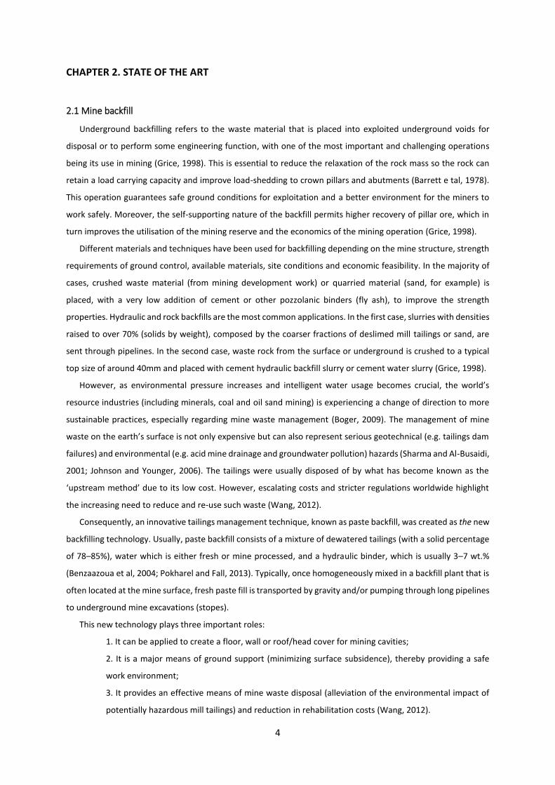
Almost all of these failures in distribution systems are associated with settling problems. For mineral
processes where a coarse solids fraction exists, there are sedimentation effects. A fraction of the particles settle
on the pipe invert, resulting in stratified flow with an asymmetric concentration and velocity profile with either
a stationary bed, or a sliding bed as illustrated in Figure 2.5. As A. J. C. Paterson explains, “As flow develops the
viscosity of the fluid in the sheared annulus decreases relative to the particle, and settling of particles in this
region occurs. As particles settle towards the invert the velocity profile changes from uniform to non-uniform,
as the point of maximum velocity is no longer at the pipe centre and moves upwards. In doing so, the effective
sheared annulus also moves upwards, and particles that were in the plug are now exposed to local shear and
begin to settle.” (Paterson, 2011).
12
Figure 2.5: Flow regimes in laminar flow (Paterson, 2011)
To avoid this settlement, the applied stress must be greater than the slurry yield stress for the material to
flow, as it will be explained subsequently.
To study the workability of paste backfill and understand its behaviour, considering paste fill as a material
fitted between moist soil and slurry, it is necessary to know rheology. Rheology is among the most important
properties of paste backfill material that determine its transportability (Ercikdi et al, 2007). This property is
present throughout the entire process of production and delivery of paste backfill, being an essential scientific
working tool for its implementation, allowing operators to solve problems and creating opportunities to make
significant improvements.
2.3 Rheology
Rheology is the science of the deformation and flow of matter (Oxford). The term was invented by Professor
Bingham of Lafayette College, Easton, and the definition was accepted when the American Society of Rheology
was founded in 1929. Due to the numerous scientific disciplines and subjects that rheology involves, significant
advances have been made in different industries over recent decades. The acceptance and application of
rheology is increasing and scientists from widely differing backgrounds are now members of national societies of
rheology in many countries (Barnes et al, 1993).
The principal theoretical concepts of rheology are related to kinematics (dealing with geometrical aspects of
deformation and flow), conservation laws, forces, stress, energy interchanges and constitutive relations. The
constitutive relations, namely, the relations between stress, strain and time for a given test sample, serve to link
motion and forces to complete the description of the flow process, which may then be applied to solve
engineering problems (He et al, 2004).
Most of the materials classified as true solids or fluids can be studied by mechanics of materials or fluid
mechanics. However, there are other special materials with no specific classification for which rheology is a very
important science in characterizing and understanding them.
In the following subchapters, relevant rheological properties (viscosity and yield stress) and concepts that
explain the difference between Newtonian and non-Newtonian materials will be introduced.
2.3.1 Rheological properties, concepts and models
Viscosity is the measure of resistance to flow, related to the internal friction of a fluid. This friction is
noticeable when a force is required to cause the physical movement or distribution of the fluid in the form of
13
pouring, spreading, spraying, mixing, etc. The greater the force required to cause this movement, denominated
“shear”, the greater the internal friction (Barnes et al, 1993, and Brookfield, 2016).
The first reference to this rheological property was made by Isaac Newton, in Principia, published in 1687:
“The resistance which arises from the lack of slipperiness of the parts of the liquid, other things being equal, is
proportional to the velocity with which the parts of the liquid are separated from one another”. The expression
“lack of slipperiness” is what we now call viscosity.
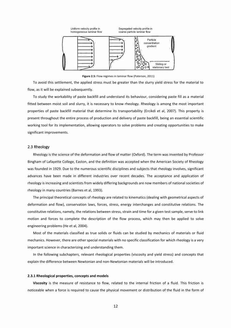
The model created by Isaac Newton (Figure 2.6) to explains this property is based on two parallel flat areas
of fluid (with an area of “A”), separated by a distance “dx”, moving in the same direction at different velocities
“V1” and “V2.”
Figure 2.6: Viscosity model by Isaac Newton (Brookfield, 2016)
Newton assumed that the force required to maintain this difference in speed was proportional to the
difference in speed through the liquid, or the velocity gradient. To express this, Newton came up with the
following expression 2.5, where 𝜂 is the viscosity constant for a given material.
𝐹
𝐴= 𝜂
𝑑𝑣
𝑑𝑥 2.5
The velocity gradient, 𝑑𝑣
𝑑𝑥 , is a measure of the change in speed at which the intermediate layers move with
respect to each other. It describes the shearing the liquid experiences and is thus called the shear rate. This is
commonly symbolised as 𝛾 and its unit of measure is the reciprocal second (sec-1).
The term 𝐹
𝐴 indicates the force per unit area required to produce the shearing action. It is referred to as shear
stress, symbolised by 𝜏 and measured by dynes per square centimetre (dynes/cm2) or Newtons per square meter
(N/m2).
Using these simplified terms, viscosity may be defined, mathematically, by expression 2.6:
𝜂 =𝜏
𝛾 2.6
The fundamental unit of viscosity measurement is the “poise” (P) (Brookfield, 2016).
Most common fluids obey Newton’s law of viscosity, which states that the shear stress 𝜏 is proportional to
the shear rate �̇�, with the proportionality constant 𝜂 called the dynamic viscosity. (Boukpeti, Nathalie et al. 2009)
A fluid that exhibits this characteristic flow behaviour (Figure 2.7) is known as a Newtonian fluid. It is, however,
only one of several types of flow behaviour that can be encountered in different fluids/materials.

14
Figure 2.7: Newtonian fluid behaviour (Brookfield, 2016)
These fluids, which exhibit an inconstant 𝜏/𝛾 relationship, are called non-Newtonian fluids and can be
identified when one of these scenarios is valid (Saebimoghaddam, 2005):
no linear relationship exists between shear stress and shear rate;
a linear relationship between shear stress and shear rate exists, but the line does not pass through the
origin;
the relationship between shear stress and shear rate demonstrates time dependency.
The viscosity of non-Newtonian fluids is variable and is alluded to as apparent viscosity (Saebimoghaddam,
2005). When it is measured, the shear rate at which the viscosity value was recorded must be noted. To better
understand this type of materials, it is worth thinking of any fluid as a mixture of molecules with different shapes
and sizes. As they pass by each other during flow, their physical characteristics determine how much force is
required to move them. At each specific rate of shear, the alignment may be different and more or less force
may be required to maintain motion. There are several types of flow behaviour, characterised by the way a fluid’s
viscosity changes in response to shear rate variations, such as:
Pseudoplastic/ shear-thinning fluid –viscosity decreasing with an increasing shear rate (Figure 2.8).
Very common in paints, emulsions and dispersions of many types;
Figure 2.8: Shear thinning fluid behaviour (Brookfield, 2016)
Dilatant/shear-thickening fluid – viscosity increasing with an increase in shear rate (Figure 2.9).
Usually found in clay slurries, candy compounds, sand/water mixtures, and others;

15
Figure 2.9: Shear thickening fluid behaviour (Brookfield, 2016)
Plastic fluid – behave as a solid under static conditions; A certain amount of stress (yield stress) must
be applied to the fluid before any flow is induced (Figure 2.10). Once this stress is exceeded and flow
begins, plastic fluids may present Newtonian, pseudoplastic or dilatant flow characteristics.
Figure 2.10: Plastic fluid behaviour (Brookfield, 2016)
Non-Newtonian fluids are also classified as thixotropic or rheopectic according to their time dependency.
When the viscosity increases with time, the fluid is rheopectic and when the viscosity decreases with time, the
fluid is thixotropic. Rheopectic fluids are very rarely encountered, however. Thixotropical behaviour is frequently
observed in materials such as greases, mineral suspensions, paints and others substances. When subjected to
varying rates of shear, a thixotropic fluid will react as illustrated in Figure 2.11. A plot of shear stress versus shear
rate show “up” and “down” curves that do not coincide. This “hysteresis loop” is caused by the decrease in the
fluid’s viscosity with increasing time of shearing. Such effects may or may not be reversible; some thixotropic
fluids, if allowed to stand undisturbed for a while, will regain their initial viscosity, while others never will
(Brookfield, 2016).
Figure 2.11: Thixotropic fluid behaviour (Brookfield, 2016)
The principal reasons that cause the time dependency of a fluid rheology are:
mixing and shearing energy input;

16
temperature and pressure changes;
progression of chemical, electrochemical and surface reactions (Li et al, 2002).
As mentioned previously, for a fluid to start flowing, it is necessary to apply a force to overcome its internal
friction. This force is related to a shear stress that deforms the particle network of the fluid. This critical shear
stress is denominated by yield stress. Theoretically, the yield stress is defined to be the stress at which the fluid
just starts/stops moving, i.e. when the viscosity changes between being finite and infinite.
For applied stresses below the yield stress, the fluid deforms elastically, with complete strain recovery upon
removal of the stress. Once the yield stress is exceeded, the material exhibits viscous liquid behaviour (Boger,
2006).
An easier way to visualise this phenomenon is given by the following expression 2.7:
{𝜎 = 𝜎𝑦 + 𝑓(�̇�) 𝑖𝑓 𝜎 > 𝜎𝑦
�̇� = 0 𝑖𝑓 𝜎 ≤ 𝜎𝑦 2.7
with 𝜎 being the applied shear stress, 𝜎𝑦 the yield stress and 𝑓(�̇�) some function of the shear rate, �̇�, satisfying
𝑓(0) = 0 and 𝑑𝑓
𝑑�̇�> 0. The Herschel-Bulkley model is a typical example of this expression and it will be presented
below (Equation 2.8).
BINGHAM PLASTIC MODEL
𝜏 = 𝜏𝑦𝐵 + 𝜂𝐵�̇� 2.8
where 𝜏𝑦𝐵 is the Bingham yield stress and the viscosity 𝜂𝐵 is defined as the slope of the shear stress-strain rate
response.
It is common for suspensions to show an apparent yield stress followed by nearly Newtonian flow above the
yield stress.
As an alternative model, the Casson model, has the same components but raised to the power of 0.5.
Consequently, it has a more gradual transition between the yield and the Newtonian regions. Because of this,
the Casson model (Equation 2.9) tends to fit better for more materials than the Bingham model (Ata scientific,
2012).
CASSON MODEL
√𝜏 = √𝜏𝑦 + √𝐾(𝛾)̇ 2.9
where 𝜏𝑦 is the yield stress and 𝐾 is the Casson viscosity, which relates to the high shear rate viscosity.
Because of the Bingham model’s simplicity, it has been widely used for yield stress materials. A refinement
of this model, which accounts for the non-linearity of the stress-strain rate behaviour, is the Herschel-Bulkley
model (Equation 2.10). This model describes non-Newtonian behaviour after yielding and is basically a power
law model with a yield stress term (Ata scientific, 2012).
HERSCHEL-BULKLEY or YIELD POWER LAW MODEL
𝜏 = 𝜏𝑦 + 𝐾�̇�𝑛 2.10
where 𝜏𝑦 = yield stress; �̇� = shear rate; 𝐾 = fluid consistency; 𝑛 = flow behaviour index or shear thinning index.

17
For a Newtonian fluid (𝑛 = 1 and 𝜏𝑦 = 0 substituted in the previous equation), the viscosity (𝐾 = 𝜂) is
represented by the slope of the rheogram, and is constant, as the function demonstrates a linear relationship
between shear stress and shear rate.
The yield power law model is usually employed for non-Newtonian (time-independent) materials. The
exponent, 𝑛, distinguishes shear thinning (𝑛 < 1) and shear thickening (𝑛 > 1) behaviour (Table 2.1).
Table 2.1: Rheological parameters of different types of non-Newtonian fluids
Behaviour 𝝉𝒚 𝒏
Pseudoplastic 0 <1
Dilatant 0 >1
Bingham plastic >0 =1
Yield pseudoplastic >0 <1
Yield dilatant >0 <1
OSTWALD-DE WAELE or POWER LAW MODEL
𝜏 = 𝐾�̇�𝑛 2.11
where 𝐾 = fluid consistency; 𝑛 = flow behaviour index
This model is applied for shear thinning and shear thickening materials (Equation 2.11). For 𝜏𝑦 = 0 in the
Herschel-Bulkley equation, the yield power law is reduced to the power law model.
To determine which model is most appropriate to describe a given material, it is necessary to measure the
steady shear stress over a range of shear rates and fit each model to the data (Figure 2.12). The correlation
coefficient is then a good indicator of proper adjustment. The range of data used in the analysis can, however,
have a bearing on the results obtained, since one model might better fit the low shear data and another the high
shear data (Ata scientific, 2012).
Figure 2.12: Shear stress versus shear rate curves for time-independent non-Newtonian slurries (He et al, 2004)
18
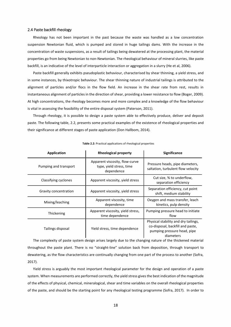
2.4 Paste backfill rheology
Rheology has not been important in the past because the waste was handled as a low concentration
suspension Newtonian fluid, which is pumped and stored in huge tailings dams. With the increase in the
concentration of waste suspensions, as a result of tailings being dewatered at the processing plant, the material
properties go from being Newtonian to non-Newtonian. The rheological behaviour of mineral slurries, like paste
backfill, is an indicative of the level of interparticle interaction or aggregation in a slurry (He et al, 2006).
Paste backfill generally exhibits pseudoplastic behaviour, characterised by shear thinning, a yield stress, and
in some instances, by thixotropic behaviour. The shear thinning nature of industrial tailings is attributed to the
alignment of particles and/or flocs in the flow field. An increase in the shear rate from rest, results in
instantaneous alignment of particles in the direction of shear, providing a lower resistance to flow (Boger, 2009).
At high concentrations, the rheology becomes more and more complex and a knowledge of the flow behaviour
is vital in assessing the feasibility of the entire disposal system (Paterson, 2011).
Through rheology, it is possible to design a paste system able to effectively produce, deliver and deposit
paste. The following table, 2.2, presents some practical examples of the existence of rheological properties and
their significance at different stages of paste application (Don Hallbom, 2014).
Table 2.2: Practical applications of rheological properties
Application Rheological property Significance
Pumping and transport Apparent viscosity, flow-curve
type, yield stress, time dependence
Pressure heads, pipe diameters, saltation, turbulent flow velocity
Classifying cyclones Apparent viscosity, yield stress Cut size, % to underflow,
separation efficiency
Gravity concentration Apparent viscosity, yield stress Separation efficiency, cut point
shift, medium stability
Mixing/leaching Apparent viscosity, time
dependence Oxygen and mass transfer, leach
kinetics, pulp density
Thickening Apparent viscosity, yield stress,
time dependence Pumping pressure head to initiate
flow
Tailings disposal Yield stress, time dependence
Physical stability and dry tailings, co-disposal, backfill and paste, pumping pressure head, pipe
diameters The complexity of paste system design arises largely due to the changing nature of the thickened material
throughout the paste plant. There is no “straight-line” solution back from deposition, through transport to
dewatering, as the flow characteristics are continually changing from one part of the process to another (Sofra,
2017).
Yield stress is arguably the most important rheological parameter for the design and operation of a paste
system. When measurements are performed correctly, the yield stress gives the best indication of the magnitude
of the effects of physical, chemical, mineralogical, shear and time variables on the overall rheological properties
of the paste, and should be the starting point for any rheological testing programme (Sofra, 2017). In order to

19
obtain relevant, robust and reproducible yield stress data for paste fill it is essential to create standard
methodologies/measurement protocols so that the mining industry and scientific community can work together
in the same direction.
A better comprehension of all paste systems (from tailings’ production to paste deposition) coupled with a
profound understanding of paste backfill properties and behaviour in different contexts is essential for solving
current problems and meeting new improvements without resorting to the “dilution solution”. Rheology is
quantitatively difficult but qualitatively easy (Don Hallbom, 2014).
2.4.1 Determinant factors
Rheological characterisation of paste fill is the measuring of the relationship between shear stress and shear
rate, varying harmonically with time. This is highly complicated and there is no single parameter that can solely
explain it. Physical and chemical properties of slurry, such as solids content, particle size, particle size distribution,
particle shape, pH value, shear rate and slurry temperature have a significant influence on the rheology of slurry
in wet ultrafine grinding (He et al., 2004).
The rheological properties are determined mostly by the solids concentration, particle size distribution, and
surface properties of the different minerals/particles. In this way, the characteristics of tailings are determinant
for paste performance. Table 2.3 presents the Golder Paste Technology (e.g, Landriault, 1995) tailings
classification system that proposes three categories (coarse, medium and fine).
Table 2.3: Tailings classification system by Golder Paste Technology
Tailings material category
Minimum passing 20
μm content (wt%)
Maximum passing 20 μm content (wt%)
Wt% solids (corresponds to 7–inch slump)
178mm slump solid
concentration CW (wt.%)
Strength development (constant w/c
ratio)
Coarse tailing 15 35 78–85 78–85 High
Medium tailing
36 60 70–78 70–78 Low
Fine tailing 61 90 55–70 55–70 Poor
From PSD curves, the following parameters can be derived: uniformity (Equation 2.12) or Harzen coefficient
(CU), coefficient of gradation (Equation 2.13) or curvature (CC), and relative span factor (Δ).
𝐶𝑢 =𝐷60
𝐷10
2.12
𝐶𝑐 =𝐷30
2
𝐷10 × 𝐷60
2.13
where 𝐷10, 𝐷30 and 𝐷60 is equal to the grain size at 10%, 30% and 60% passing, respectively.
For paste backfill of the good quality expected, the suitable tailings material must be well graded (Figure
2.13). Gradation describes the distribution of different size groups within a tailings sample. Well-graded tailings
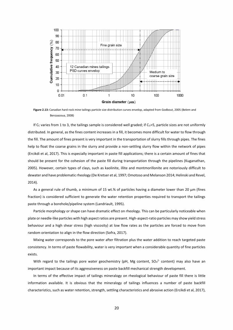
contain all sizes of material (Belem et al, 2008).
20
Figure 2.13: Canadian hard rock mine tailings particle size distribution curves envelop, adapted from Godbout, 2005 (Belem and
Benzaazoua, 2008)
If CC varies from 1 to 3, the tailings sample is considered well graded; if CU>5, particle sizes are not uniformly
distributed. In general, as the fines content increases in a fill, it becomes more difficult for water to flow through
the fill. The amount of fines present is very important in the transportation of slurry fills through pipes. The fines
help to float the coarse grains in the slurry and provide a non-settling slurry flow within the network of pipes
(Ercikdi et al, 2017). This is especially important in paste fill applications; there is a certain amount of fines that
should be present for the cohesion of the paste fill during transportation through the pipelines (Kuganathan,
2005). However, certain types of clays, such as kaolinite, illite and montmorillonite are notoriously difficult to
dewater and have problematic rheology (De Kretser et al, 1997; Omotoso and Melanson 2014; Helinski and Revel,
2014).
As a general rule of thumb, a minimum of 15 wt.% of particles having a diameter lower than 20 μm (fines
fraction) is considered sufficient to generate the water retention properties required to transport the tailings
paste through a borehole/pipeline system (Landriault, 1995).
Particle morphology or shape can have dramatic effect on rheology. This can be particularly noticeable when
plate or needle-like particles with high aspect ratios are present. High-aspect-ratio particles may show yield stress
behaviour and a high shear stress (high viscosity) at low flow rates as the particles are forced to move from
random orientation to align in the flow direction (Sofra, 2017).
Mixing water corresponds to the pore water after filtration plus the water addition to reach targeted paste
consistency. In terms of paste flowability, water is very important when a considerable quantity of fine particles
exists.
With regard to the tailings pore water geochemistry (pH, Mg content, SO42- content) may also have an
important impact because of its aggressiveness on paste backfill mechanical strength development.
In terms of the effective impact of tailings mineralogy on rheological behaviour of paste fill there is little
information available. It is obvious that the mineralogy of tailings influences a number of paste backfill
characteristics, such as water retention, strength, settling characteristics and abrasive action (Ercikdi et al, 2017),

21
but it is not clear how they specifically impact on rheological matters. However, chemical composition of tailings
is of most importance for the mechanical strength development of paste backfill.
2.4.2 Yield stress
Yield stress is the critical shear stress that must be exceeded before irreversible deformation and flow can
occur. For applied stress below the yield stress, the particle network of the suspension deforms elastically, with
complete strain recovery upon removal of the stress. The yield stress profile (the yield stress as a function of
solids concentration and cement content) is the single most important data set for the design and operation of
paste systems (Sofra, 2017).
Once the yield stress is exceeded, the suspension exhibits viscous liquid behaviour where the viscosity is
usually a decreasing function of the shear rate. This property of paste fill is extremely important for pipeline and
thickener designs. Due to the lack of mineral suspension data at low shear rates, a common practice is to
extrapolate the linear portion (shear stress vs. shear rate) to the y-axis and refer to this as the yield stress. This
is a Bingham yield stress measurement that bears no relationship whatsoever to the true yield stress of the
material (Figure 2.14). The linear portion of the curve being fitted in this way is sometimes appropriate for
pipeline design, but yield stress determined in this way is far from adequate for the design of a thickener.
Figure 2.14: Typical flow curves. (a) Newonian; (b) Bingham (yield-constant plastic viscosity); (c) yield-pseudoplastic (shear thinning);
(d) yield dilatant (shear thickening)
The most complicated non-Newtonian behaviour, which can be observed in mineral and associated
industries, is time-dependent behaviour. Here, the shear stress is a function of both shear rate and time of shear
(Boger, 2006). Basically, this is the case where the alignment of the particles and/or flocs occurs on a timescale
that can be observed in the rheometer.
There has been an ongoing debate in the literature as to whether true yield stress fluids exist, and even
whether the concept is useful. This is mainly due to the difficulties in determining the yield stress experimentally,
and the usefulness and pertinence of the concept in different contexts. The precise yield stress of a given
material, as a true material constant, has turned out to be very difficult to measure, as different tests often give

22
different results. Even in controlled rheology experiments this problem is well documented: “depending on the
measurement geometry and the detailed experimental protocol, very different values of the yield stress may be
found” (James et al, 1987; Nguyen & Boger, 1992; Barnes, 1997,1999; Barnes & Nguyen 2001).
Consequently, there is no universal method for determining yield stress, but there are a large number of
approaches, which find favour across different industries and establishments (Ata scientific, 2012).
To this end, an international inter-laboratory, involving six laboratories, has been set up to evaluate the
reliability and reproducibility of several common yield stress measuring techniques employed in different
laboratories, and with different instruments, using aqueous suspensions of colloidal TiO2 at concentrations of
40–70 wt% solids. The details of the experimental materials and techniques employed by the participants are
summarised in Table 2.4.
Table 2.4: Details of experimental materials and techniques used in the inter-laboratory study
Laboratory Samples tested
Sample preparation
Technique Instrumentation Sample
conditioning
Q.D. Nguyen (University of
Adelaide, Australia)
TiO2 suspension 40–60 wt%
solids
Mechanical agitation 2hrs
@300 rpm, rested 24 hrs, pH 6.9
Steady-shear measurement extrapolation
Stress–controlled rheometer Bohlin CVO50,
vane-cup geometry
Thoroughly mixed for 10 mins
Stress ramp Creep test
Stress–controlled rheometer Bohlin CVO50,
vane-cup
Presheared at 100 s-1 for 5 mins
Vane technique Rate–controlled
rheometer Haake RT55, vane device
Thoroughly mixed for 10 mins
H. Usui (Kobe University, Japan)
TiO2 suspension 50–60 wt%
solids
Mechanical stirring 1hr @100 rpm, pH
7.0
Steady-shear measurement extrapolation
Rate–controlled rheometer Iwamoto
Seisakusho IR200, cone-plate
Restirred 1 min
Shear stress ramp Stress–controlled
rheometer Rheometric SR-5, cone-plate
Presheared 10 mins at 31 s-1,
rested 10 s
C. Tiu (Monash University, Australia)
TiO2 suspension 50–60 wt%
solids
Mechanical agitation 24hrs pH
7.0
Steady-shear measurement extrapolation
Rate–controlled rheometer Haake RV20,
grooved bob-cup
Presheared 10 mins at 10 s-1, rested 10 mins
Stress ramp Creep test
Stress–controlled rheometer Rheometric
DSR, vane-cup
Presheared 10 mins at 10 s-1, rested 10 mins
Vane technique Rate–controlled
rheometer Haake RV20, vane device
Presheared 10 mins at 10 s-1, rested 10 mins
Static equilibrium Cylindrical penetrometer Presheared 10 min at 10 s-1, rested 10 min
D. De Kee (Tulane, University, USA)
TiO2 suspension 40–70 wt%
solids
Stirring with spatula 1 hr, pH 7.0
Steady-shear measurement extrapolation
Stress–controlled rheometer SR5000, plate-
plate Restirred 1 min
P. Coussot (Laboratoire des Matériaux et des
Structures du Génie Civil, France)
TiO2 suspension 50–60 wt%
solids
Mechanical stirring at least 1 hr, pH 7.0
Static equilibrium Inclined plane device Thoroughly mixed
D.V. Boger (University of Melbourne,
Australia)
TiO2 suspension 60
wt% solids
Sonication 2 min, pH 7.7
Vane technique Rate–controlled
rheometer Haake RE50, vane device
Hand-stirred 1min
The yield stress results provided by different laboratories suggested that the measured yield stress varies
with both methods and participants. Among the different techniques employed, direct methods were found to

23
produce more reliable and repeatable results than indirect methods. A statistical analysis of the data from four
different laboratories clearly indicated that the repeatability of yield stress measurements using different
methods within any given laboratory was much better than the reproducibility among different laboratories
(Nguyen, 2005).
In some applications, one method that has been frequently used for characterizing yield stress materials is to
work with two yield stresses - one static and one dynamic – or even a whole range of yield stresses (Mujumbar
et al, 2002 and references therein). It depends at which moment the measure is taken and/or the procedure
adopted (Figure 2.15). The static yield stress is the stress above which the material turns from a solid state to a
liquid one (usually higher in value), while the dynamic yield stress is the stress where the material turns from a
liquid state to a solid one. In another words, the dynamic yield stress is the minimum stress required for
maintaining flow. It is usually better to measure the static yield stress when looking at initiating flow in a material
i.e. pumping (Ata scientific, 2012).
Nevertheless, for practical applications, the yield stress is accepted as the highest stress at which no flow is
detectable for the duration of the experiment.
Figure 2.15: Different yield stress values during shearing (Moller et al, 2006)
Yet viewed from a more theoretical perspective, many authors argue that most of these difficulties disappear
when a clear distinction is made between two types of yield stress fluids: thixotropic and simple. A simple yield
stress fluid is one for which the shear stress (and hence the viscosity) depends only on the shear rate, while for
thixotropic fluids the viscosity depends also on the shear history of the sample. In other words, thixotropic
materials can change structurally with time of applied shear and/or take a finite time to recover after yielding
(Ata scientific, 2012).
The distinction is simple to make, in principle: one can, for instance, measure the flow curve by using an up-
and-down stress ramp. If the material is a “normal” yield stress fluid, the data for increasing and decreasing shear
stresses coincide: the material parameters do not depend on flow history. On the other hand, if the material is
thixotropic, in general the flow will have significantly “liquefied” the material at high stresses, and the branch
obtained upon decreasing the stress is significantly below the one obtained while increasing the stress (Moller,
Peter et al, 2009). From this perspective, for normal yield stress fluids there is no problem in determining the

24
yield stress, but for thixotropic materials there is, since any flow liquefies the material and thus decreases the
yield stress. As thixotropy is, both by definition and in practice, reversible, which also means that when it is left
at rest after shearing, the yield stress will increase again. The aforementioned inter-laboratory study also noted
that “a lack of proper control of the shear history and time-dependent effects in thixotropic suspensions may
also contribute to the poor reproducibility of yield stress measurements using any technique.” (Nguyen et al,
2005)
Despite the questions surrounding yield stress measurements and concepts, many researchers and engineers
accept and often choose this variable to work with. As Nguyen and Boger (1992) affirm, “Despite the
controversial concept of the yield stress as a true material property (…) there is generally acceptance of its
practical usefulness in engineering design and the operation of processes where handling and transport of
industrial suspensions are involved” (Moller et al, 2006).
For all these reasons, it is clear that there is a need for the standardisation of procedures not only for yield
stress measurements (taking the shear history of the samples into account), but also for the
preparation/conditioning of the specimens. The test methods should be adequate and representative as much
as possible to the conditions under which the paste will flow and how exactly it will flow. Once the objective is
identified, sample selection, preparation and testing conditions must be determined to ensure that information
gained through testing will be applicable for design. With the rheology of paste systems being particularly
sensitive to numerous physical and chemical/mineralogical factors, this is not always a trivial exercise (Sofra,
2017).
2.4.3 Measurement methodologies
Accurate rheological measurements are critical to understanding the rheology of paste backfill. The ability to
correctly measure rheological properties, as opposed to a “relative” value, enables proper design and operation
that can be applied across a range of materials of varying physical properties.
These techniques can be classified as direct and indirect methods according to the value if they are named as
“apparent” (accurate techniques) or “extrapolated” (non-absolute techniques), respectively (Nguyen and Boger,
1992).
2.4.3.1 Indirect methods
In general, indirect methods refer to the measurement of yield stress with extrapolation of shear stress-shear
rate data and direct methods are involved in the independent assessment of yield stress and viscosity. The
empirical rheological models describing the shear stress (𝜏) –shear rate (�̇�) dependence of non-Newtonian
mineral slurries are Bingham plastic, Casson, Herschel–Bulkley and Ostwald-de-Waele models. These models
were previously presented and explained in chapter 2.3.1.
This method of extrapolation is very straightforward and, as has been discussed before, the yield stress
determined in this way is far from adequate and can result in gross overdesign for the design of paste tailings
dewatering systems, tailings/cement mixing requirements or pumping and pipeline design (Sofra and Boger
1991).

25
2.4.3.2 Direct methods
Direct methods are involved in the independent assessment of yield stress, and the measured value can be
referred to as “true” yield stress, describing the critical shear stress when the fluid begins to flow
(Saebimoghaddam, 2005). A growing number of techniques have been developed over recent decades to
measure these properties for paste technology. Most of them are an adaptation from other industries such as
concrete. To determine yield stress and viscosity, the apparatus must be able to measure the paste’s ability to
start flowing and to flow once applied stress exceeds yield stress, respectively (Belem et al, 2007).
2.4.3.2.1 Slump
In an attempt to further simplify yield stress measurement, the “slump test” has been modified to accurately
evaluate the yield stress of mineral suspensions (Showalter and Christensen, 1998; Pashias et al, 1996; Boger et
al, 2002). This technique has typically been used to determine the empirical flow characteristics of fresh concrete,
in another words, to estimate the workability or consistency of fresh concrete. Nowadays, this is a usual method
for mine backfilling control (Figure 2.16). Most of the consultant companies recommend this method for
evaluating the workability of the paste and establishing slump intervals for each mine/case of application. Slump
height, an empirical measure of consistency, is dependent on both material yield stress and density, which are
in turn dependent on chemical composition, particle specific gravity, and particle size. In the minerals industry,
these factors may vary with changes in ore origin and processing (Belem et al, 2007).
The slump test is conducted using an ASTM standard slump cone, eliminating the need for sophisticated
equipment and allowing easy, on-site yield stress measurement by plant operators.
Equation 2.14, for evaluating the yield stress from a slump height measurement, is given by:
𝜏′𝑦 =1
2+
1
2√𝑆′ 2.14
where 𝜏′𝑦 is the yield stress dimensionalised with respect to 𝜌𝑔ℎ; 𝑆′ is the dimensional slump measurement,
which is dimensionalised with ℎ, the height of the slump cylinder; 𝜌 is the density of the suspension; and 𝑔 is the
acceleration due to gravity.
Despite the simplicity of this test, some factors may influence the results, such as the sensibility of the
operator, the time to fill the cone and the surface inclination, among others. Thus, using the slump height as the
single parameter of consistency for paste backfill distribution systems potentially leads to problems (Clayton et
al, 2003).

26
Figure 2.16: Slump test carried out at the Neves-Corvo and Zinkgruvan paste plants on 14/09/2015 and 21/12/2016 respectively
2.4.3.2.2 Flow table
The flow table, like slump, is a very common tool in determining cement mortar consistency. This equipment
is chosen for concrete where the nominal maximum size of aggregate does not exceed 38mm. The cone mould
is firmly held on the centre of the table and filled with the sample in two layers. Each layer is compacted by 25
strokes with a tamping rod, in a uniform manner over the cross section of the mould. After the top layer has
been rodded, the mould is then removed from the concrete by a steady upward pull. The table is raised and
dropped from a height of 12.5mm, 15 times per second. The diameter of the spread is the average of two
diameters (approximately right-angled).
2.4.3.2.3 Inclined plane test
Coussot and Boyer (1995) proposed a method to determine yield stress from the inclined plane test, using a
1 metre-long (D) channel with width L varying between 5 cm and 25 cm and slope (i) varying between 100 and
300. The bottom surface was plywood. The authors demonstrated that wall slip is negligible for mud flows on this
surface type, and they successfully compared measured uniform flow depths (h) with theoretical predictions
(based on rheometrical tests). They also observed no flow depth change when using surfaces with different
roughness. Asymptotic depth (ℎ0), corresponding to at rest state (final position or equilibrium), leads to the
determination of yield stress (Equation 2.15):
𝜏𝑦 = 𝜌𝑔ℎ0sin (𝑖) 2.15
where 𝜌 = material bulk density (𝑘𝑔/𝑚3), 𝑔 = gravitational acceleration (𝑚/𝑠2); ℎ0 = final height of material
(𝑚); and 𝑖 = inclined plane slope angle.
2.4.3.2.4 Cylindrical penetrometer
Ulherr et al (2002) developed a novel and simple method for measuring yield stress using a cylindrical
penetrometer. Basically, static equilibrium of a falling penetrometer in a yield stress fluid (partial immersion) is
measured, and uniform shear stress acting on the entire penetrometer surface is assumed. Yield stress is simply
determined by a balance of forces acting on the penetrometer (Equation 2.16), as follows (Belem et al, 2007):

27
𝜏𝑦 =𝑔 [𝑚𝑝 − 𝜌𝜋𝑑2 (
14
+𝑑
12)]
𝜋𝑑 (𝑙 +𝜋𝑑8
) 2.16
where 𝑔 = gravitational acceleration (𝑚/𝑠2); 𝑚𝑝 = total mass of the penetrometer (𝑘𝑔); 𝜌 = fluid bulk density
(𝑘𝑔/𝑚3); and 𝑑 and 𝑙 are the diameter (𝑚) and immersed length (𝑚) of the cylindrical section of the
penetrometer.
The above equation indicates that yield stress is a function of the weight and dimensions of the immersed
penetrometer. Thus, yield stress is readily determined by measuring equilibrium depth in the fluid for a
penetrometer with known weight and diameter (Belem et al, 2007).
2.4.3.2.5 Fall cone instrument
The fall cone technique has been employed in many fields of engineering and in other industries. The
operating principle is quite simple: a standard cone is released from a certain height and allowed to drop freely
into the sample. A graduated scale attached to the frame permits the penetration of the plunger to be measured.
The penetration, expressed in mm, is the result of a constant force (equal to the cone’s weight) applied to the
top horizontal surface of the material. While the cone is entering the fluid, the surface area of shear between
the cone and the fluid increases, and consequently the shear stress decreases. The yield stress can be considered
at the equilibrium state of the shear stress, and the yield stress of the fluid where the cone stops penetrating can
be determined by the Equation 2.17 (Saebimoghaddam, 2005):
𝜏𝑦 =𝐾𝐹
𝑍2 2.17
where F is the force (including the weight of cone), Z is the indentation depth and K is a geometrical factor and
may be determined from the Equation 2.18,
𝐾 =(𝑐𝑜𝑡𝜃)2
𝜋 2.18
where 2𝜃 is the cone angle.
It has been mentioned that this method is most suitable for a fluid material with a high yield stress or low
viscosity due to the minimal effect of viscous resistance to penetration of the cone. On the other hand, the lower
the penetration time the more reliable the yield stress value (Nguyen and Boger, 1992).
2.4.3.2.6 Rheometry / viscometry
Rheometers and viscometers are pieces of equipment for directly measuring of the relationship between
shear rate and shear stress or apparent viscosity, which characterises the slurry rheology (He et al, 2004).
Viscometers measure the viscosity and flow properties of a fluid at a particular shear rate. Rheometers are more
sophisticated and measure the way a fluid responds to applied shear or stress, potentially providing data on
material structure and elasticity.
Three basic types of this equipment that been tried for slurry applications: concentric cylinder/rotational,
capillary tube and cone and plate viscometers/rheometers.

28
Concentric cylinder or rotational instruments, such as Bohlin instruments, Brookfield viscometers, Haake
viscometers, TA instruments and Debex viscometers, are very popular in research laboratories (Nguyen and
Boger, 1992; Slatter 1997; Slatter, 2004). Their measurement technique consists of a rotating inner cylinder
(bob/spindle) and a stationary hollow cylinder (cup). Torque is required for rotating the spindle at a constant
rotational speed (Ω) when fluid is located between the cup and the bob. The torque is related to shear stress,
and the rotational speed is related to shear rate. Extrapolation of data to zero shear rate from such an instrument
is generally not a good way to determine the yield stress. This type of rheometer/viscometer is simple to operate,
not expensive, widely accepted, compact (can be installed as a “bench-top” instrument), requires small samples
and can be measure time dependency.
Capillary tube instruments have been used and recommended by several engineers in the mining industry
(Cooke & Paterson, 1996; Cooke, 2001; Slatter, 2004). The fluid flows at a constant velocity V through a tube
with a length L and an inside diameter D, which demonstrates exactly what may happen in a pipeline fluid
transportation system (Saebimoghaddam, 2005). It can be used larger tubes for coarse slurry (D ten times higher
than the particle size). It is not possible to measure time–dependent properties because there is a unique
function between shear rate and shear stress. The problems associated with this type of measuring are
turbulence, radical particle migration, segregation at entrance and wall slip (interaction between the particles
and the tube wall), among others.
Cone and plate instruments are based on the same concentric cylinder principle, where the bob has the
geometry of a cone or plate and rotates. The fluid is sheared within the gap. A torque (T) is required to rotate
the cone or plate at the constant angular velocity (Ω), and the rheological parameters are given as follows
(Equation 2.19 and 2.20):
�̇�(𝑟) = 𝑓(𝜏) =Ω
𝑡𝑎𝑛𝜃 2.19
and
𝜏 =3𝑇
2𝜋𝑅3 2.20
where 𝜃 is the cone angle and R is the cone radius. In this equipment, both shear stress and shear rate are
constant and can be calculated directly from torque and cone angle, which is its advantage. There are several
commercial types of this equipment with a different range of shear rate, usually from 10−3 to 103 𝑠−1. The cone
and plate device is not very suitable for all types of fluids due to a small gap requirement. The alternative case
for the cone is a truncated cone, and can be used for suspensions where the minimum gap is at least ten times
greater than the largest particle size (Nguyen and Boger 1992).
The following technique also relates to viscometry/rheometry, as since the vane geometry can be used as a
bob/spindle attached to this type of equipment.
2.4.3.2.7 Vane-shear instrument and technique
The vane-shear instrument and technique allows direct and accurate determination of the yield stress from
a single point measurement (Nguyen, 1983; Nguyen and Boger, 1983, 1985). Many workers worldwide have
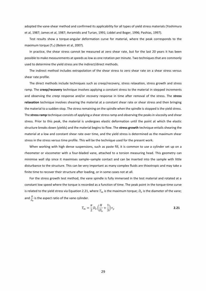
29
adopted the vane-shear method and confirmed its applicability for all types of yield stress materials (Yoshimura
et al, 1987; James et al, 1987; Avramidis and Turian, 1991; Liddel and Boger, 1996; Pashias, 1997).
Test results show a torque-angular deformation curve for material, where the peak corresponds to the
maximum torque (Tm) (Belem et al, 2007).
In practice, the shear stress cannot be measured at zero shear rate, but for the last 20 years it has been
possible to make measurements at speeds as low as one rotation per minute. Two techniques that are commonly
used to determine the yield stress are the indirect/direct methods.
The indirect method includes extrapolation of the shear stress to zero shear rate on a shear stress versus
shear rate profile.
The direct methods include techniques such as creep/recovery, stress relaxation, stress growth and stress
ramp. The creep/recovery technique involves applying a constant stress to the material in stepped increments
and observing the creep response and/or recovery response in time after removal of the stress. The stress
relaxation technique involves shearing the material at a constant shear rate or shear stress and then bringing
the material to a sudden stop. The stress remaining on the spindle when the spindle is stopped is the yield stress.
The stress ramp technique consists of applying a shear stress ramp and observing the peaks in viscosity and shear
stress. Prior to this peak, the material is undergoes elastic deformation until the point at which the elastic
structure breaks down (yields) and the material begins to flow. The stress growth technique entails shearing the
material at a low and constant shear rate over time, and the yield stress is determined as the maximum shear
stress in the stress versus time profile. This will be the technique used for the present work.
When working with high dense suspensions, such as paste fill, it is common to use a cylinder set up on a
rheometer or viscometer with a four-bladed vane, attached to a torsion measuring head. This geometry can
minimise wall slip since it maximises sample–sample contact and can be inserted into the sample with little
disturbance to the structure. This can be very important as many complex fluids are thixotropic and may take a
finite time to recover their structure after loading, or in some cases not at all.
For the stress growth test method, the vane spindle is fully immersed in the test material and rotated at a
constant low speed where the torque is recorded as a function of time. The peak point in the torque-time curve
is related to the yield stress via Equation 2.21, where 𝑇𝑚 is the maximum torque; 𝐷𝑣 is the diameter of the vane;
and 𝐻
𝐷𝑣 is the aspect ratio of the vane cylinder.
𝑇𝑚 =𝜋
2𝐷𝑣 (
𝐻
𝐷𝑣
+1
3) 𝜏𝑦 2.21

30
CHAPTER 3. EXPERIMENTAL WORK
This chapter summarises the physical and chemical characteristics of different samples of tailings and the
experimental testing programme carried out in this work: specimen preparation, mixing, mix design calculation,
test methods and procedures.
Initially, a practice run was carried out using both mine tailings samples to define the mixtures designs, to
choose/adapt the necessary equipment and to establish the techniques and procedures to be employed. This
preliminary work was very important in recognising the materials to be tested and gain some experience in
dealing with the equipment/instruments and their operation/procedure methods. In addition to this, an attempt
was made to develop/adapt an apparatus capable of accurately measuring the yield stress of fresh paste fill in
the lab, in a test that could be transferred to the field. After some research and various attempts, the fall cone
instrument was chosen and adapted. All of the relevant information about this will be presented subsequently.
3.1Mine tailings
The tested tailings were obtained from two mines: Neves-Corvo (Portugal) and Zinkgruvan (Sweden). Both of
the tailings samples were collected in the disc filters at the paste plant of each mine, and kept inside barrels (45
l). Subsequently, the barrels were sent to the GeoLab at Tecnico Lisboa, Portugal, where they have been tested.
3.1.1 Zinkgruvan Mine, Sweden
Zinkgruvan Mine is located approximately 250 km southwest of Stockholm in south-central Sweden, with
good road access and close to the main E18 highway linking the cities of Stockholm and Oslo. This mine is 100%
owned and operated by Lundin Mining Corporation, a base metals mining company, through its Swedish
subsidiary Zinkgruvan Mining AB.
The deposit has been known since the 16th century and large scale production began in 1857 and has
continued uninterrupted ever since. Zinkgruvan Mining AB holds a total area for exploitation concessions of
679ha (covering the deposit and its surroundings) and exploration licences for a total área of 3,753 ha.
Geologically, the Zinkgruvan orebodies are massively dominated by layers of sphalerite and galena,
intercalated with barren layers of quarzitic metatuffite and calc-silicate rock. Layers of disseminated sphalerite
and galena occur locally towards the hanging wall. Galena is locally remobilised into veins, particularly in the
Knalla Mine. Remobilisation of galena and silver has occurred in response to metamorphism and deformation,
and is most pronounced in the lead-rich western extension of Nygruvan and in the Burkland area
(http://www.lundinmining.com/s/Zinkgruvan.asp).
Paste backfill technology was introduced in 2001.
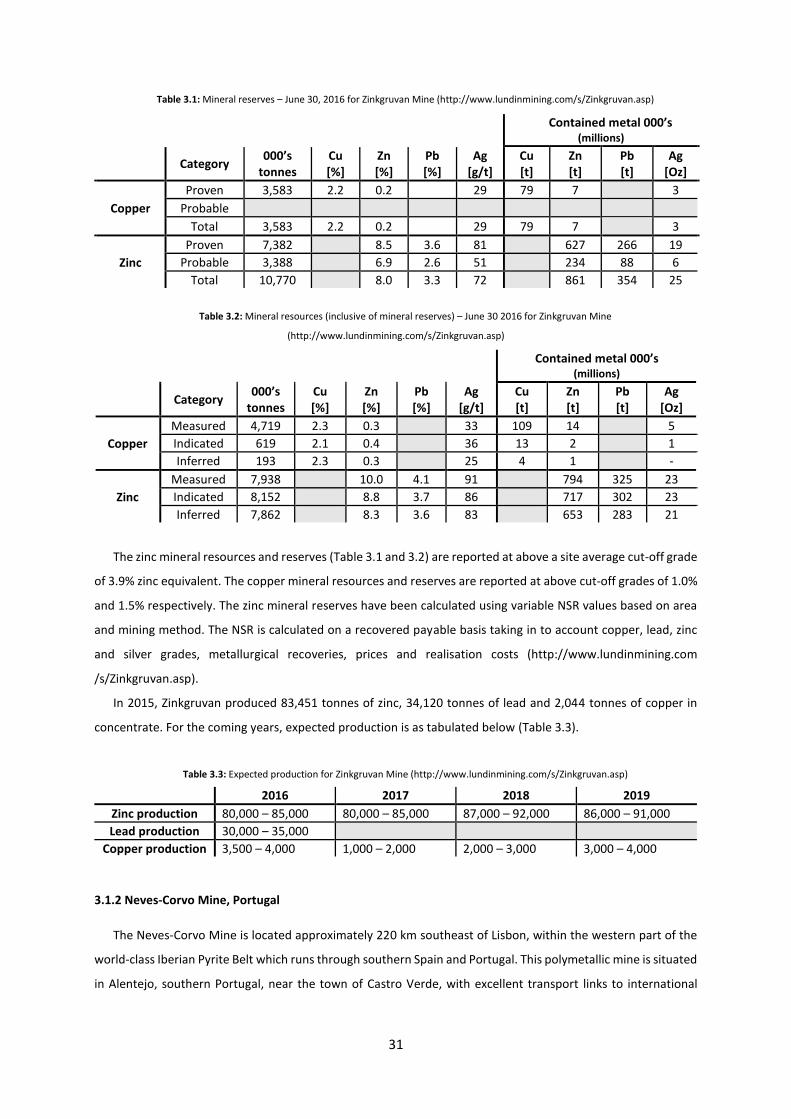
31
Table 3.1: Mineral reserves – June 30, 2016 for Zinkgruvan Mine (http://www.lundinmining.com/s/Zinkgruvan.asp)
Contained metal 000’s (millions)
Category
000’s tonnes
Cu [%]
Zn [%]
Pb [%]
Ag [g/t]
Cu [t]
Zn [t]
Pb [t]
Ag [Oz]
Copper
Proven 3,583 2.2 0.2 29 79 7 3
Probable
Total 3,583 2.2 0.2 29 79 7 3
Zinc
Proven 7,382 8.5 3.6 81 627 266 19
Probable 3,388 6.9 2.6 51 234 88 6
Total 10,770 8.0 3.3 72 861 354 25
Table 3.2: Mineral resources (inclusive of mineral reserves) – June 30 2016 for Zinkgruvan Mine
(http://www.lundinmining.com/s/Zinkgruvan.asp)
Contained metal 000’s (millions)
Category
000’s tonnes
Cu [%]
Zn [%]
Pb [%]
Ag [g/t]
Cu [t]
Zn [t]
Pb [t]
Ag [Oz]
Copper
Measured 4,719 2.3 0.3 33 109 14 5
Indicated 619 2.1 0.4 36 13 2 1
Inferred 193 2.3 0.3 25 4 1 -
Zinc
Measured 7,938 10.0 4.1 91 794 325 23
Indicated 8,152 8.8 3.7 86 717 302 23
Inferred 7,862 8.3 3.6 83 653 283 21
The zinc mineral resources and reserves (Table 3.1 and 3.2) are reported at above a site average cut-off grade
of 3.9% zinc equivalent. The copper mineral resources and reserves are reported at above cut-off grades of 1.0%
and 1.5% respectively. The zinc mineral reserves have been calculated using variable NSR values based on area
and mining method. The NSR is calculated on a recovered payable basis taking in to account copper, lead, zinc
and silver grades, metallurgical recoveries, prices and realisation costs (http://www.lundinmining.com
/s/Zinkgruvan.asp).
In 2015, Zinkgruvan produced 83,451 tonnes of zinc, 34,120 tonnes of lead and 2,044 tonnes of copper in
concentrate. For the coming years, expected production is as tabulated below (Table 3.3).
Table 3.3: Expected production for Zinkgruvan Mine (http://www.lundinmining.com/s/Zinkgruvan.asp)
2016 2017 2018 2019
Zinc production 80,000 – 85,000 80,000 – 85,000 87,000 – 92,000 86,000 – 91,000
Lead production 30,000 – 35,000
Copper production 3,500 – 4,000 1,000 – 2,000 2,000 – 3,000 3,000 – 4,000
3.1.2 Neves-Corvo Mine, Portugal
The Neves-Corvo Mine is located approximately 220 km southeast of Lisbon, within the western part of the
world-class Iberian Pyrite Belt which runs through southern Spain and Portugal. This polymetallic mine is situated
in Alentejo, southern Portugal, near the town of Castro Verde, with excellent transport links to international
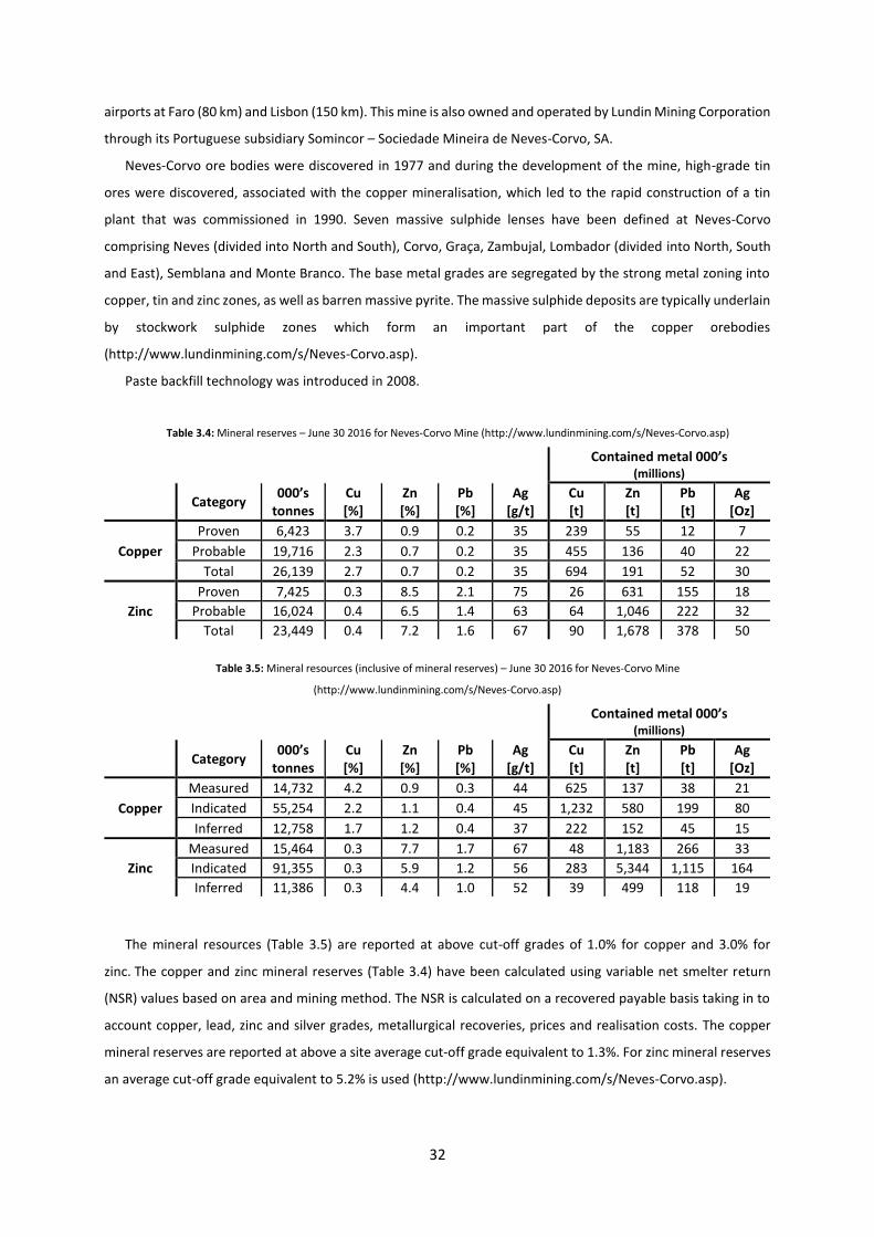
32
airports at Faro (80 km) and Lisbon (150 km). This mine is also owned and operated by Lundin Mining Corporation
through its Portuguese subsidiary Somincor – Sociedade Mineira de Neves-Corvo, SA.
Neves-Corvo ore bodies were discovered in 1977 and during the development of the mine, high-grade tin
ores were discovered, associated with the copper mineralisation, which led to the rapid construction of a tin
plant that was commissioned in 1990. Seven massive sulphide lenses have been defined at Neves-Corvo
comprising Neves (divided into North and South), Corvo, Graça, Zambujal, Lombador (divided into North, South
and East), Semblana and Monte Branco. The base metal grades are segregated by the strong metal zoning into
copper, tin and zinc zones, as well as barren massive pyrite. The massive sulphide deposits are typically underlain
by stockwork sulphide zones which form an important part of the copper orebodies
(http://www.lundinmining.com/s/Neves-Corvo.asp).
Paste backfill technology was introduced in 2008.
Table 3.4: Mineral reserves – June 30 2016 for Neves-Corvo Mine (http://www.lundinmining.com/s/Neves-Corvo.asp)
Contained metal 000’s
(millions)
Category 000’s
tonnes Cu [%]
Zn [%]
Pb [%]
Ag [g/t]
Cu [t]
Zn [t]
Pb [t]
Ag [Oz]
Copper
Proven 6,423 3.7 0.9 0.2 35 239 55 12 7
Probable 19,716 2.3 0.7 0.2 35 455 136 40 22
Total 26,139 2.7 0.7 0.2 35 694 191 52 30
Zinc
Proven 7,425 0.3 8.5 2.1 75 26 631 155 18
Probable 16,024 0.4 6.5 1.4 63 64 1,046 222 32
Total 23,449 0.4 7.2 1.6 67 90 1,678 378 50
Table 3.5: Mineral resources (inclusive of mineral reserves) – June 30 2016 for Neves-Corvo Mine
(http://www.lundinmining.com/s/Neves-Corvo.asp)
Contained metal 000’s
(millions)
Category 000’s
tonnes Cu [%]
Zn [%]
Pb [%]
Ag [g/t]
Cu [t]
Zn [t]
Pb [t]
Ag [Oz]
Copper
Measured 14,732 4.2 0.9 0.3 44 625 137 38 21
Indicated 55,254 2.2 1.1 0.4 45 1,232 580 199 80
Inferred 12,758 1.7 1.2 0.4 37 222 152 45 15
Zinc
Measured 15,464 0.3 7.7 1.7 67 48 1,183 266 33
Indicated 91,355 0.3 5.9 1.2 56 283 5,344 1,115 164
Inferred 11,386 0.3 4.4 1.0 52 39 499 118 19
The mineral resources (Table 3.5) are reported at above cut-off grades of 1.0% for copper and 3.0% for
zinc. The copper and zinc mineral reserves (Table 3.4) have been calculated using variable net smelter return
(NSR) values based on area and mining method. The NSR is calculated on a recovered payable basis taking in to
account copper, lead, zinc and silver grades, metallurgical recoveries, prices and realisation costs. The copper
mineral reserves are reported at above a site average cut‐off grade equivalent to 1.3%. For zinc mineral reserves
an average cut‐off grade equivalent to 5.2% is used (http://www.lundinmining.com/s/Neves-Corvo.asp).

33
In 2015, Neves-Corvo produced 55,831 tonnes of copper and 61,921 tonnes of zinc in concentrate. For the
coming years, expected production is as tabulated below (Table 3.6).
Table 3.6: Expected production for Neves-Corvo Mine (http://www.lundinmining.com/s/Neves-Corvo.asp)
2016 2017 2018 2019
Copper production 50,000 – 55,000 41,000 – 46,000 42,000 – 47,000 45,000 – 50,000
Zinc production 65,000 – 70,000 72,000 – 77,000 70,000 – 75,000 66,000 – 71,000
3.1.3 Physical and chemical characterisation of mine tailings
The following analysis is intended to characterise the physical and chemical properties of Neves-Corvo and
Zinkgruvan mine tailings. This was undertaken by the Corporate Analytic Service of Sika Technology AG (R&D
Department).
As mentioned earlier, the tailings received from each mine were sealed in 4 barrels. The sampling of
Zinkgruvan tailings was carried out in March 2016, and the Neves-Corvo tailings on 16 November 2016.
For the particle size distribution analysis, a sample of each barrel was analysed. For the chemical analysis,
one sample of Neves-Corvo tailings named S1, corresponding to barrel 1, and two samples of Zinkgruvan tailings
named Z1 and Z3, corresponding to the barrels 1 and 3, were analysed.
3.1.3.1 Particle size distribution
The particle size distribution (PSD) analysis was done using the laser diffraction technique, using equipment
Sympatec HELOS equipment & dry dispersion in air stream (RODOS). Each sample was manually sieved by a mesh
size of 1mm, to separate big agglomerates. The particle size was evaluated in dry mode (compressed air,
horizontal flow) with the laser granulometry. The dispersing of the powder occurs through particle-to-particle
collisions, particle-to-wall collisions and centrifugal forces due to strong velocity gradients (Tzschichholz, 2017).
Cumulative and density distributions of Neves-Corvo and Zinkgruvan barrels are shown in Figure 3.1 and 3.2,
respectively. Each PSD curve represents a single combined measurement.
Figure 3.1: Cumulative and density distributions of the 4 barrels of Neves-Corvo tailings

34
Figure 3.2: Cumulative and density distributions of the 4 barrels of Zinkgruvan tailings
Overall, the difference between the tailings from the two mines is clear. Zinkgruvan tailings are much coarser
than Somincor tailings, showing an accentuated slope of the curve starting in 20/30 μm of particle size. In terms
of the differences between barrels, PSD curves for the Somincor barrels are similar to each other, proving that
they were collected at the same time. In contrast, for the Zinkgruvan barrels the PSD curves show a clear
difference between barrels 1/2 and 3/4, suggesting that the tailings were collected on separate days. It is also
possible that barrel 4 may not have been collected at the same time as barrel 3, due to a slight difference in the
maximum values of the curves.
The characteristic diameters of the cumulative distribution (D10, D30, D50, D60, D90), the percentage of material
passing under 20 μm, the uniformity coefficient, Cu, and the coefficient of gradation, Cc, values are presented in
Table 3.7.
Table 3.7: The size distribution characteristics of Somincor and Zinkgruvan tailings
Sample D10 [μm] D30 [μm] D50 [μm] D60 [μm] D90 [μm] < 20 μm [%] Cc Cu
S1 4.0 20.4 43.5 58.5 157.9 29.8 1.78 14.63
S2 3.8 19.7 42.8 57.7 151.9 30.4 1.77 15.18
S3 3.7 19.3 42.5 56.7 150.1 30.9 1.78 15.32
S4 3.7 19.9 44.2 59.3 160.8 30.2 1.80 16.03
Z1 7.6 43 75.7 95 207.2 17.1 2.56 12.5
Z2 8.0 43.5 75.8 95 204.4 16.7 2.49 11.88
Z3 10.1 50 89.7 118 254.1 14.8 2.10 11.68
Z4 9.4 48 84.8 109 236.5 15.4 2.25 11.60
These values corroborated the analysis made through the observation of cumulative and density
distributions.
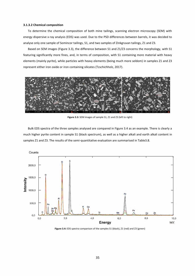
35
3.1.3.2 Chemical composition
To determine the chemical composition of both mine tailings, scanning electron microscopy (SEM) with
energy dispersive x-ray analysis (EDS) was used. Due to the PSD differences between barrels, it was decided to
analyse only one sample of Somincor tailings, S1, and two samples of Zinkgruvan tailings, Z1 and Z3.
Based on SEM images (Figure 3.3), the difference between S1 and Z1/Z3 concerns the morphology, with S1
featuring significantly more fines, and, in terms of composition, with S1 containing more material with heavy
elements (mainly pyrite), while particles with heavy elements (being much more seldom) in samples Z1 and Z3
represent either iron oxide or iron containing silicates (Tzschichholz, 2017).
Figure 3.3: SEM images of sample S1, Z1 and Z3 (left to right)
Bulk EDS spectra of the three samples analysed are compared in Figure 3.4 as an example. There is clearly a
much higher pyrite content in sample S1 (black spectrum), as well as a higher alkali and earth alkali content in
samples Z1 and Z3. The results of the semi-quantitative evaluation are summarised in Table3.8.
Figure 3.4: EDS spectra comparison of the samples S1 (black), Z1 (red) and Z3 (green)

36
Table 3.8: Semi-quantitative evaluation of the element content (expressed as oxide) in S1, Z1 and Z3 samples
Element oxide Element oxide content in weight [%]
S1 Z1 Z3
Na2O n.d. 0,1 ± 0,1 0,3 ± 0,2
MgO 1,5 ± 0,2 4,3 ± 0,2 4,0 ± 0,3
Al2O3 6,6 ± 0,2 12,0 ± 0,1 12,9 ± 0,2
SiO2 19,6 ± 1,0 49,6 ± 0,9 54,9 ± 0,6
SO3 37,7 ± 1,1 3,0 ± 0,3 2,5 ± 0,4
K2O 0,5 ± 0,1 5,2 ± 0,1 6,2 ± 0,1
CaO 0,7 ± 0,1 7,4 ± 0,3 7,5 ± 0,2
TiO2 n.d. 0,6 ± 0,2 0,7 ± 0,3
MnO n.d. 1,0 ± 0,1 0,7 ± 0,2
Fe2O3 31,3 ± 0,5 15,0 ± 0,2 8,8 ± 0,3
CuO 1,0 ± 0,2 n.d. n.d.
ZnO 1,2 ± 0,1 1,6 ± 0,3 1,7 ± 0,3
3.1.3.3 Mineralogy
To determine the mineralogy of the samples, the x-ray diffraction on powder (XRD) method was employed,
with Bruker D8 ADVANCE equipment. The samples analysed were the same as the chemical composition (S1, Z1
and Z3).
The agglomerates (> 1 mm) of three tailings samples were pestled and sieved (< 63 μm). The samples were
manually prepared and measured over the angle range 2θ 3°-65° with a step size of 0.013° and 1s measuring
time per step-high resolution (Table 3.9).
The phase analysis was carried out by Bruker software TOPAS 4 using Rietveld calculation with standard errors
of around 2% (absolute). The phase composition of the three tailings is given in Table 3.10, where the values are
presented in percentage of weight.
Table 3.9: Sieve fraction of sample S1, Z1 and Z3
S1 Z1 Z3
Total amount 40.05 g 40.00 g 40.00 g
< 63 μm 25.80 g (64.4%) 18.05 g (45.1%) 14.75 g (36.9%)
> 63 μm 13.97 g (34.9%) 21.69 g (54.2%) 25.08 g (62.7%)
Table 3.10: Quantitative phase analysis (Rietveld) of sieved tailings (< 63 μm)
Phase Formula S1 Z1 Z3
Quartz SiO2 39.4 18.8/17.6 31.4/27.2
Magnetite Fe3O4 (< 0.5) 1.7/1.4 < 0.5/1.2
Pyrite FeS2 38.1 – –
Chalcopyrite CuFeS2 0.9 1.8/1.6 –
Galena/galenite PbS – 0.6/0.8 < 0.5
Siderite FeCO3 3.1 – –
Muscovite Biotite
KAl2AlSi3O10(OH)2 K(Mg,Fe)3AlSi3O10(OH)2
8.2 (< 0.5)
7.5/10.3 7.9/1.5
1.9/7.1 7.9/4.6
Chlorite (Mg,Fe,Al)6(Si,Al)4O10(OH) 8.3 10.3/10.8 6.9/7.7
Epidote Ca2Fe3+Al2(Si2O7)(SiO4)O(OH) 2.0 (–) (–)

37
Calcite CaCO3 – – 3.0/4.8
Dolomite CaMg(CO3)2 – 1.2/3.4 < 0.5/1.8
Albite NaAlSi3O8 (< 0.5) 2.0/7.1 5.8/10.3
Orthoclase/microcline KAlSi3O8 – 21.9/21.3 24.7/24.5
Cordierite Mg2Al4Si5O18 – 13.1/12.2 4.1/9.5
Diopside (pyroxene) CaMgSi2O6 – 13.0/12.0 9.3/1.0
Enstatite (pyroxene) Mg2Si2O6 – – 4.4/ –
unknown ? X X X
3.2 Testing design
3.2.1 Specimen preparation
Due to the sedimentation of the particles inside the Zinkgruvan barrels, the material of each barrel was
transferred to another, bigger-barrel, and continually mixed with a drill mixing paddle (Figure 3.5). This way the
homogenisation of the tailings was guaranteed.
Figure 3.5: Tailings homogenisation
From this point, the tailings from each barrel were divided into eleven samples of approximately 4 kilograms
and sealed in plastic bags (to prevent evaporation). Ten of these samples were used to produce paste to be
tested at the GeoLab, while one was to be sent for physical and chemical analysis (Figure 3.6).
Figure 3.6: Tailings separated in 11 bags from Zinkgruvan Mine (barrel 2)
The barrels received from Neves-Corvo mine were split on the day after sampling (Figure 3.7). The material
was split into small samples, as done with Zinkgruvan tailings.

38
Figure 3.7: Tailings of 4 barrels separated in 44 bags from Neves-Corvo Mine
To measure the water content of each sample/bag, the tailings were mixed (for homogenisation) by a Hobart
mixer and then a small specimen 𝑊𝑠, was taken to be weighed and dried in the oven for 24 hours at 800C.
Figure 3.8: Tailings weighing and drying oven
The weight of the tailings (sample/bag) were accurately measured and then preserved inside a plastic box to
avoid evaporation (Figure 3.8). The very next day, the specimen was weighed again, 𝐷𝑠, and the water content
calculated by the equation 3.1:
𝑊𝑎𝑡𝑒𝑟 𝑐𝑜𝑛𝑡𝑒𝑛𝑡 (%) =𝑊𝑠 − 𝐷𝑠
𝑊𝑠
3.1
Knowing this value and the total weight of the sample (inside the plastic box), it was possible to calculate the
quantity of cement and water to be added to make the desired mixture (Figure 3.9).
Figure 3.9: Samples of Zinkgruvan barrel 3 ready to mix, after water content measurement
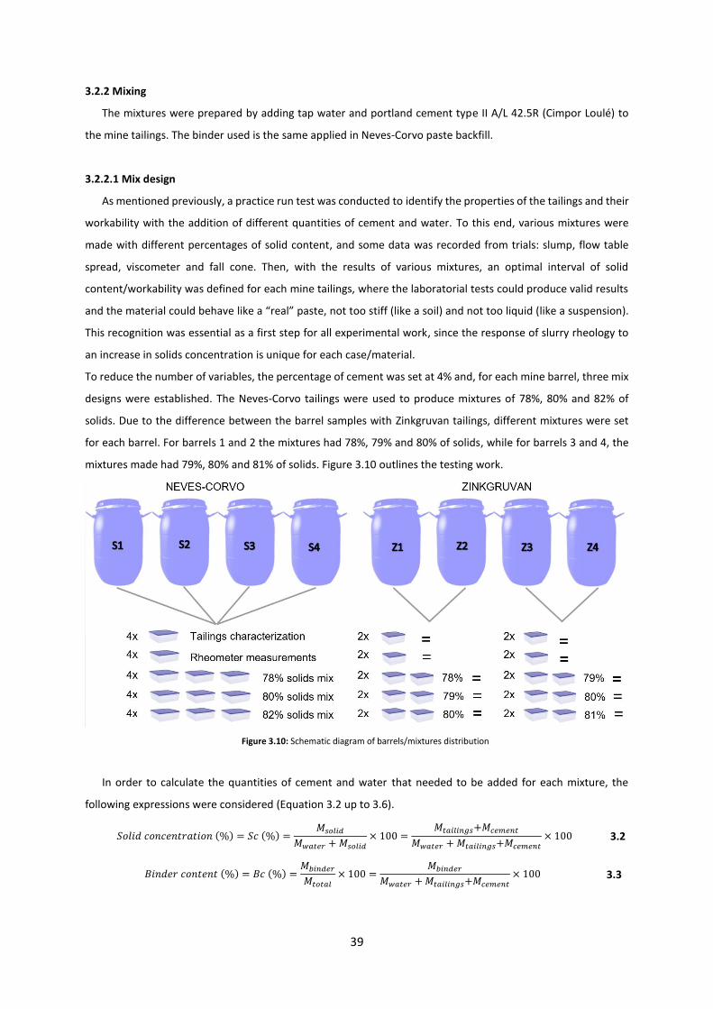
39
3.2.2 Mixing
The mixtures were prepared by adding tap water and portland cement type II A/L 42.5R (Cimpor Loulé) to
the mine tailings. The binder used is the same applied in Neves-Corvo paste backfill.
3.2.2.1 Mix design
As mentioned previously, a practice run test was conducted to identify the properties of the tailings and their
workability with the addition of different quantities of cement and water. To this end, various mixtures were
made with different percentages of solid content, and some data was recorded from trials: slump, flow table
spread, viscometer and fall cone. Then, with the results of various mixtures, an optimal interval of solid
content/workability was defined for each mine tailings, where the laboratorial tests could produce valid results
and the material could behave like a “real” paste, not too stiff (like a soil) and not too liquid (like a suspension).
This recognition was essential as a first step for all experimental work, since the response of slurry rheology to
an increase in solids concentration is unique for each case/material.
To reduce the number of variables, the percentage of cement was set at 4% and, for each mine barrel, three mix
designs were established. The Neves-Corvo tailings were used to produce mixtures of 78%, 80% and 82% of
solids. Due to the difference between the barrel samples with Zinkgruvan tailings, different mixtures were set
for each barrel. For barrels 1 and 2 the mixtures had 78%, 79% and 80% of solids, while for barrels 3 and 4, the
mixtures made had 79%, 80% and 81% of solids. Figure 3.10 outlines the testing work.
Figure 3.10: Schematic diagram of barrels/mixtures distribution
In order to calculate the quantities of cement and water that needed to be added for each mixture, the
following expressions were considered (Equation 3.2 up to 3.6).
𝑆𝑜𝑙𝑖𝑑 𝑐𝑜𝑛𝑐𝑒𝑛𝑡𝑟𝑎𝑡𝑖𝑜𝑛 (%) = 𝑆𝑐 (%) =𝑀𝑠𝑜𝑙𝑖𝑑
𝑀𝑤𝑎𝑡𝑒𝑟 + 𝑀𝑠𝑜𝑙𝑖𝑑× 100 =
𝑀𝑡𝑎𝑖𝑙𝑖𝑛𝑔𝑠+𝑀𝑐𝑒𝑚𝑒𝑛𝑡
𝑀𝑤𝑎𝑡𝑒𝑟 + 𝑀𝑡𝑎𝑖𝑙𝑖𝑛𝑔𝑠+𝑀𝑐𝑒𝑚𝑒𝑛𝑡× 100 3.2
𝐵𝑖𝑛𝑑𝑒𝑟 𝑐𝑜𝑛𝑡𝑒𝑛𝑡 (%) = 𝐵𝑐 (%) =𝑀𝑏𝑖𝑛𝑑𝑒𝑟
𝑀𝑡𝑜𝑡𝑎𝑙× 100 =
𝑀𝑏𝑖𝑛𝑑𝑒𝑟
𝑀𝑤𝑎𝑡𝑒𝑟 + 𝑀𝑡𝑎𝑖𝑙𝑖𝑛𝑔𝑠+𝑀𝑐𝑒𝑚𝑒𝑛𝑡× 100 3.3

40
𝑀𝑎𝑠𝑠 𝑜𝑓 𝑏𝑖𝑛𝑑𝑒𝑟 (𝑔) =𝐵𝑐
100× 𝑀𝑡𝑜𝑡𝑎𝑙 =
𝐵𝑐
100× (𝑀𝑡𝑜𝑡𝑎𝑙 + 𝑀𝑐𝑒𝑚𝑒𝑛𝑡 + 𝑀𝑑𝑟𝑦𝑡𝑎𝑖𝑙𝑖𝑛𝑔𝑠) 3.4
𝑀𝑎𝑠𝑠 𝑜𝑓 𝑑𝑟𝑦 𝑡𝑎𝑖𝑙𝑖𝑛𝑔𝑠 (𝑔) = 𝑀𝑡𝑜𝑡𝑎𝑙 × (𝑆𝑐
100) − 𝑀𝑐𝑒𝑚𝑒𝑛𝑡 = (𝑀𝑤𝑎𝑡𝑒𝑟 + 𝑀𝑑𝑟𝑦𝑡𝑎𝑖𝑙𝑖𝑛𝑔𝑠+𝑀𝑐𝑒𝑚𝑒𝑛𝑡) × (
𝑆𝑐
100) − 𝑀𝑐𝑒𝑚𝑒𝑛𝑡 3.5
𝑀𝑎𝑠𝑠 𝑜𝑓 𝑊𝑎𝑡𝑒𝑟(𝑔) = 𝑀𝑡𝑜𝑡𝑎𝑙 − 𝑀𝑐𝑒𝑚𝑒𝑛𝑡 − 𝑀𝑑𝑟𝑦𝑡𝑎𝑖𝑙𝑖𝑛𝑔𝑠 3.6
As previously explained, the tailings were wet and the water content, 𝑊𝑐(%), was determined as well as the
weight of each tailings sample. Therefore, the previous expressions are given as (Equation 3.7 and 3.8):
𝑀𝑎𝑠𝑠 𝑜𝑓 𝑤𝑒𝑡 𝑡𝑎𝑖𝑙𝑖𝑛𝑔𝑠 (𝑔) = 𝑀𝑑𝑟𝑦𝑡𝑎𝑖𝑙𝑖𝑛𝑔𝑠 + 𝑀𝑑𝑟𝑦𝑡𝑎𝑖𝑙𝑖𝑛𝑔𝑠 × (𝑊𝑐
100) 3.7
𝑀𝑎𝑠𝑠 𝑜𝑓 𝑤𝑎𝑡𝑒𝑟 (𝑔) = 𝑀𝑡𝑜𝑡𝑎𝑙 × (𝑆𝑐
100) − 𝑀𝑐𝑒𝑚𝑒𝑛𝑡 = (𝑀𝑤𝑎𝑡𝑒𝑟 + 𝑀𝑑𝑟𝑦𝑡𝑎𝑖𝑙𝑖𝑛𝑔𝑠+𝑀𝑐𝑒𝑚𝑒𝑛𝑡) × (
𝑆𝑐
100) − 𝑀𝑐𝑒𝑚𝑒𝑛𝑡 3.8
3.2.2.2 Procedure
The mixing procedure combined different rotational speeds, agitators and mixing times. First, the tailings
were placed inside the mixer bowl and mixed for 1 minute using the flat beater at speed 1. The flat beater was
then substituted by the whip attachment and the water was slowly added at speed 1. After 1 minute of mixing,
the cement was slowly added. At last, the final mixture was mixed at speed 2 for 3 minutes to ensure that the
materials were well blended by the Hobart mixer.
Between the laboratorial tests, the mixture was placed inside the mixer bowl and remixed using the whip
attachment at speed 2 for 1 minute to adjust and replace the sample for testing (and guarantee the paste
homogeneity).
3.2.3 Test methods and procedures
After mixing the trials were done in the following order: dry content, bulk density, viscometer, rheometer,
fall cone (300 and 600), flow table and slump. The rheometer measurements were done with an Anton Paar
RheolabQC instrument, generously provided by the Geomechanical Laboratory at Neves-Corvo Mine.
3.2.3.1 Bulk density
The bulk density is defined as the mass of a bulk material (such as paste) divided by the volume occupied by
that material.
This property was measured in all mixtures using a plastic container with a volume, v, of 125 ml and a
weight,𝑐, of 20g. The procedure adopted is similar to the standards ASTM C138/C 138M-01a and BS EN 12350-6
2009. After mixing, the paste was placed inside the container in two layers of approximately equal volume. Each
layer was rodded with 25 strokes, to release the entrapped air, and the final top surface levelled. Finally, the
container filled with paste was weighed, p, and the bulk density calculated by the Equation 3.9.
𝐷𝑒𝑛𝑠𝑖𝑡𝑦 (𝑘𝑔/𝑚3) =𝑝 − 𝑐
𝑣 3.9
3.2.3.2 Dry Content
Dry content is defined as the ratio between the mass of a sample of the material after drying and its mass at
the time of sampling (it is expressed as a percentage). The standard followed was the SCAN-P 39:80.
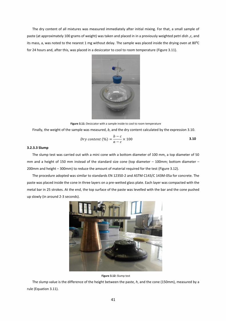
41
The dry content of all mixtures was measured immediately after initial mixing. For that, a small sample of
paste (at approximately 100 grams of weight) was taken and placed in in a previously weighted petri dish ,c, and
its mass, a, was noted to the nearest 1 mg without delay. The sample was placed inside the drying oven at 800C
for 24 hours and, after this, was placed in a desiccator to cool to room temperature (Figure 3.11).
Figure 3.11: Desiccator with a sample inside to cool to room temperature
Finally, the weight of the sample was measured, b, and the dry content calculated by the expression 3.10.
𝐷𝑟𝑦 𝑐𝑜𝑛𝑡𝑒𝑛𝑡 (%) =𝑏 − 𝑐
𝑎 − 𝑐× 100 3.10
3.2.3.3 Slump
The slump test was carried out with a mini cone with a bottom diameter of 100 mm, a top diameter of 50
mm and a height of 150 mm instead of the standard size cone (top diameter – 100mm; bottom diameter –
200mm and height – 300mm) to reduce the amount of material required for the test (Figure 3.12).
The procedure adopted was similar to standards EN 12350-2 and ASTM C143/C 143M-05a for concrete. The
paste was placed inside the cone in three layers on a pre-wetted glass plate. Each layer was compacted with the
metal bar in 25 strokes. At the end, the top surface of the paste was levelled with the bar and the cone pushed
up slowly (in around 2-3 seconds).
Figure 3.12: Slump test
The slump value is the difference of the height between the paste, h, and the cone (150mm), measured by a
rule (Equation 3.11).

42
𝑆𝑙𝑢𝑚𝑝 (𝑚𝑚) = 150 − ℎ 3.11
3.2.3.4 Flow table
To measure the slump-flow, using a flow table for cement mortar, a cone with a bottom diameter of 100mm,
a top diameter of 70mm and height of 50mm was used (Figure 3.13).
The procedure adopted was similar to standard ASTM C230 for cement mortar. The cone was centrally placed
on the pre-wetted table and filled with paste in two layers. Each layer was compacted with the metal bar of
slump in 25 strokes. After this, the top surface of the paste was levelled with the bar and the cone lifted (in
around 1 second). In the end, the table was mechanically dropped 15 times (one drop per second). The diameter
of the paste was measured twice: at the beginning (after the cone lifting) and at the end (after the 15 strokes
made with the up and down movement of the table). For both, two straight diameters were measured (Equation
3.12).
𝐼𝑛𝑖𝑡𝑖𝑎𝑙 𝑑𝑖𝑎𝑚𝑒𝑡𝑒𝑟 (𝑚𝑚) = 𝐹𝑖𝑛𝑎𝑙 𝑑𝑖𝑎𝑚𝑒𝑡𝑒𝑟 (𝑚𝑚) =𝑑1 + 𝑑2
2 3.12
Figure 3.13: Flow table test
3.2.3.5 Vane method
The absolute values of yield stress and viscosity were determined in a controlled shear rate mode (stress
growth technique), CSR, by a viscometer and a rheometer with vane spindles.
3.2.3.5.1 Viscometer
The measurement of yield stress and viscosity was done by the DV1 Brookfield rotational viscometer, model
RV, with four-blade vanes (V73 and V75) and the Wingather SQ software, V4.0.7 (Figure 3.14 and 3.15). The paste
samples were tested inside a 600 mL low form Griffin beaker, the standard sample container for most Brookfield
viscometers.

43
Figure 3.14: DV1 Brookfield rotational viscometer and vane spindles
After the mixing, the paste is placed inside the beaker up to the 500 ml mark. The spindle, already attached
to the viscometer, is gently inserted and centred into the paste until the primary immersion mark of the spindle
is achieved. For the measurements, the viscometer was programmed for a constant speed of 0.3 rpm and a
running time of 2 minutes and 15 seconds. The software recorded the data (torque, rpm, time and viscosity) at
a time interval of 3 seconds.
Figure 3.15: Wingather SQ software
In order to convert the torque values (%) measured by the viscometer into shear stress (Pa) values, the
following formulation, Equation 3.13, is given by Brookfield Engineering Labs:
𝜏 =𝑀
2𝜋𝑅𝑏2𝐿
3.13
where 𝑅𝑏 is the radius of spindle (V73=0.6335cm and V75=0.4015cm), 𝐿 is the length of spindle (V73=2.535cm
and V75=1.61 cm) and 𝑀 is the torque input by instrument (dyne-cm). In this case, as the viscometer is a RV
series, it has a spring torque of 7187 dyne-cm. The torque (dyne-cm) is equal to the multiplication of the torque
value recorded (%) by 7187.
3.2.2.5.2 Rheometer
The measurement of the yield stress with the rheometer was done with an Anton Paar RheolabQC instrument
with the vane spindle ST22-6V-16 and Rheoplus software V3.62 (Figure 3.16).

44
Figure 3.16: Anton Paar RheolabQC instrument, paste sample inside the container and vane spindle (from left to right)
The technique used was the same that was followed with the viscometer. The major difference relates to the
speed. In this case, the rheometer was programmed for a constant speed of 0.1 rpm for a running time of 3
minutes and 20 seconds. The software recorded the data every second and the yield stress value considered
was the highest shear stress value measured.
3.2.2.6 Fall cone
Besides these laboratory tests, an attempt was made to develop/adapt an apparatus able to accurately
measure the yield stress of fresh paste fill in the laboratory or in the field. After some research and attempts, the
fall cone instrument was chosen, which is well known in soil mechanics for measuring the liquid and plastic limit
of soils. There are already some studies about the possibility of measuring the yield stress of undrained soils and,
more recently, of colloidal TiO2 suspensions using a similar method (cylindrical penetrometer), but not for paste
fill specifically.
During the practice run, some experiments were carried out with the available fall cone equipment (Controls
S.R.L. instrument) at the university laboratory, using a standard metal cone of 30 degrees (Figure 3.17). Due to
the height of the cone (too heavy), the cone became completely immersed in the samples at every attempt.
Figure 3.17: Fall cone instrument and standard steel cone
Thus, it was decided to recreate the exact geometry of the metal cone (and the bar attached) with a lighter
material. After some unsuccessful reproductions, two final prototypes were printed in a Formlabs 3D printer, at

45
the maximum possible definition (0.025mm) with a special resin for top quality output, durability and toughness.
The cones were printed with 30 and 60 degrees, weighing 12g and 18 g respectively (Figures 3.18 and 3.19).
Figure 3.18: Formlabs 3D printer, on the left, and the cones printed with 600 and 300 degrees, on the right
A container was filled with paste and the top surface levelled with a spatula. The cone was positioned at the
top of the container, with the point of the cone slightly touching the surface of the paste. The cone was dropped
and, after penetration, the measurement was made as quickly as possible. The main difference between this
procedure and the standard method applied to soils is the time of penetration. Since it is intended to correlate
to the penetration with the yield stress, the sooner the penetration depth is measured, the better the correlation
will be.
The containers used had a 53 mm diameter and a height of 68mm for the 30-degree cone, and a 85mm
diameter and a height of 75mm for the 60-degree cone.
Figure 3.19: Printed cones, positioned on the fall cone instrument

46
CHAPTER 4. RESULTS AND DATA ANALYSIS
In this chapter, the experimental work results are presented followed by some descriptions and observations.
A total of 72 mixtures were produced, 36 using each mine tailings. From these mixtures, the viscosity and yield
stress were determined using seven different test methods: the slump, the flow table (initial and final diameter),
the fall cone (30 and 60 degrees), the viscometer and the rheometer. The number of values recorded is over 500.
In order to simplify the observation of the results obtained, the values presented in the tables of this chapter are
the average of the numbers recorded for each mixture design/test method. All of the values obtained are
presented in Annexes I and II.
The following sub-chapters are organised by test method, starting with the vane method. This method was
applied using two pieces of equipment: a viscometer and a rheometer. The values of viscosity (only measured by
the viscometer) and yield stress are presented in two tables along with the average of shear stress-time curves.
The results of the other test methods are subsequently presented in tables and graphs of correlation with the
dry content of the mixtures and with the yield stress values recorded by both pieces of equipment.
When observing the dry content values ini Annexes I and II, it is worth noting that these don’t correspond to
the solid content of mix designs. In Zinkgruvan mixtures, these differences are more evident (about 4%)
compared to Neves-Corvo mixtures (about 2%). The reasons for this variance may be associated with errors in
determining the tailings water content and the mixtures’ dry content. Furthermore, as the mineralogy of both
tailings is significantly different, the water present inside the particles may be different, as may the time and
temperature necessary to evaporate this water. However, the dry content values are consistent for each mix
design and from now on these will be taken into account for the presentation or discussion of results.
4.1 Vane method
Several measurements were carried out to determine the yield stress values of Zinkgruvan and Neves-Corvo
paste fill mixtures. To this end, a controlled shear rate mode was applied using a viscometer and a rheometer
with adaptable vane spindles. The yield stress recorded corresponds to the maximum values of the shear stress-
time curves obtained.
4.1.1 DV1 Brookfield viscometer
Using the DV1 Brookfield viscometer, the viscosity and the yield stress of all mixtures were measured at room
temperature and a rotational speed of 0.3 rpm. The viscosity values (Pa.s) recorded correspond to the point of
maximum torque. To convert the torque values into shear stress values, Equation 3.13 previously presented in
the experimental work chapter, was applied. Due to the shear stress reading range of each vane spindle, for
Zinkgruvan mixtures the V73 spindle (range of 10-100 Pa) was applied, while for Neves-Corvo mixtures, the V75
spindle (range of 40-400 Pa) was used. The results are shown in Table 4.1.
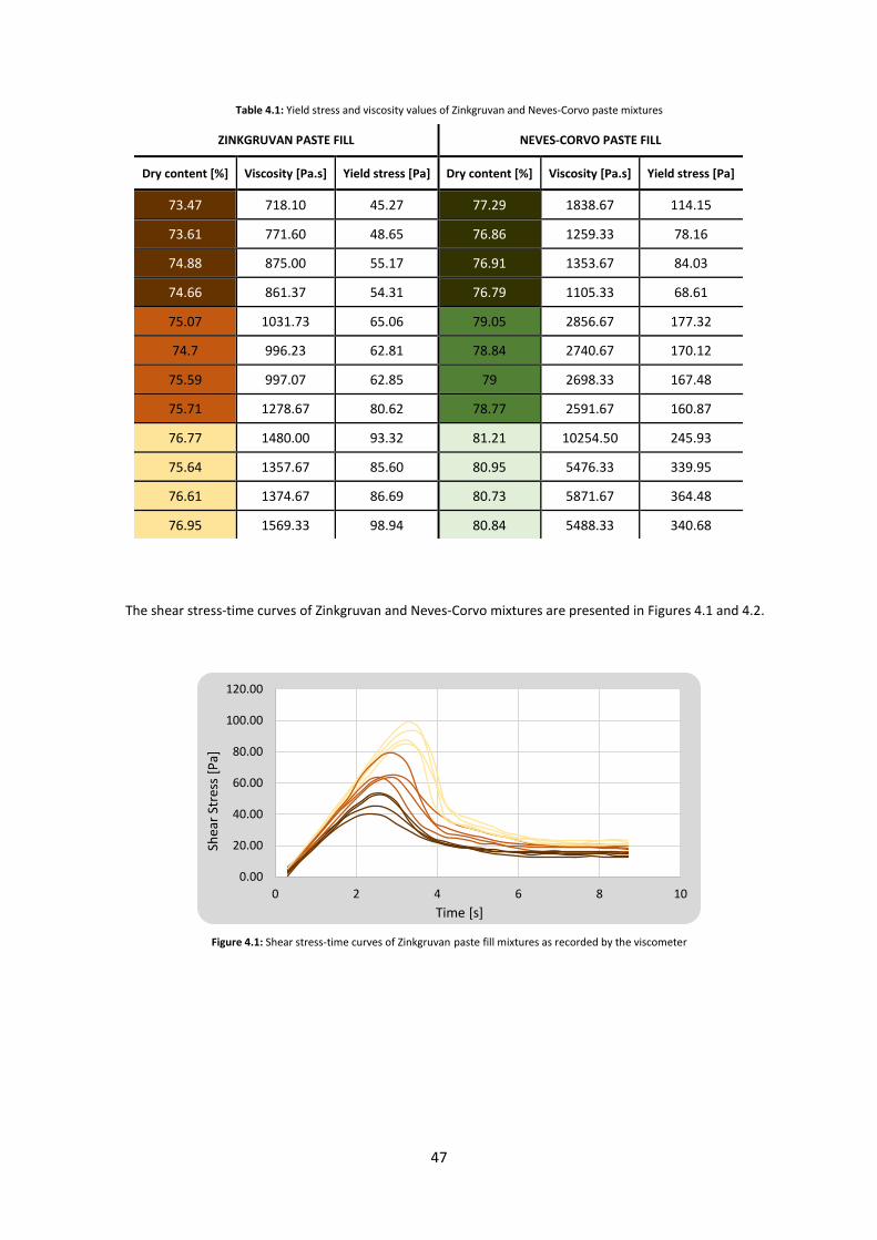
47
Table 4.1: Yield stress and viscosity values of Zinkgruvan and Neves-Corvo paste mixtures
The shear stress-time curves of Zinkgruvan and Neves-Corvo mixtures are presented in Figures 4.1 and 4.2.
Figure 4.1: Shear stress-time curves of Zinkgruvan paste fill mixtures as recorded by the viscometer
0.00
20.00
40.00
60.00
80.00
100.00
120.00
0 2 4 6 8 10
Shea
r St
ress
[P
a]
Time [s]
ZINKGRUVAN PASTE FILL NEVES-CORVO PASTE FILL
Dry content [%] Viscosity [Pa.s] Yield stress [Pa] Dry content [%] Viscosity [Pa.s] Yield stress [Pa]
73.47 718.10 45.27 77.29 1838.67 114.15
73.61 771.60 48.65 76.86 1259.33 78.16
74.88 875.00 55.17 76.91 1353.67 84.03
74.66 861.37 54.31 76.79 1105.33 68.61
75.07 1031.73 65.06 79.05 2856.67 177.32
74.7 996.23 62.81 78.84 2740.67 170.12
75.59 997.07 62.85 79 2698.33 167.48
75.71 1278.67 80.62 78.77 2591.67 160.87
76.77 1480.00 93.32 81.21 10254.50 245.93
75.64 1357.67 85.60 80.95 5476.33 339.95
76.61 1374.67 86.69 80.73 5871.67 364.48
76.95 1569.33 98.94 80.84 5488.33 340.68
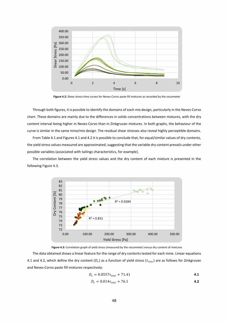
48
Figure 4.2: Shear stress-time curves for Neves-Corvo paste fill mixtures as recorded by the viscometer
Through both figures, it is possible to identify the domains of each mix design, particularly in the Neves-Corvo
chart. These domains are mainly due to the differences in solids concentrations between mixtures, with the dry
content interval being higher in Neves-Corvo than in Zinkgruvan mixtures. In both graphs, the behaviour of the
curve is similar in the same mine/mix design. The residual shear stresses also reveal highly perceptible domains.
From Table 4.1 and Figures 4.1 and 4.2 it is possible to conclude that, for equal/similar values of dry contents,
the yield stress values measured are approximated, suggesting that the variable dry content prevails under other
possible variables (associated with tailings characteristics, for example).
The correlation between the yield stress values and the dry content of each mixture is presented in the
following Figure 4.3.
Figure 4.3: Correlation graph of yield stress (measured by the viscometer) versus dry content of mixtures
The data obtained shows a linear feature for the range of dry contents tested for each mine. Linear equations
4.1 and 4.2, which define the dry content (𝐷𝑐) as a function of yield stress (𝜏𝑣𝑖𝑠𝑐) are as follows for Zinkgruvan
and Neves-Corvo paste fill mixtures respectively:
𝐷𝑐 = 0.0557𝜏𝑣𝑖𝑠𝑐 + 71.41 4.1
𝐷𝑐 = 0.014𝜏𝑣𝑖𝑠𝑐 + 76.1 4.2
0.00
50.00
100.00
150.00
200.00
250.00
300.00
350.00
400.00
0 2 4 6 8 10
Shea
r St
ress
[P
a]
Time [s]
R² = 0.831
R² = 0.9284
72
73
74
75
76
77
78
79
80
81
82
83
0.00 100.00 200.00 300.00 400.00 500.00
Dry
Co
nte
nt
[%]
Yield Stress [Pa]
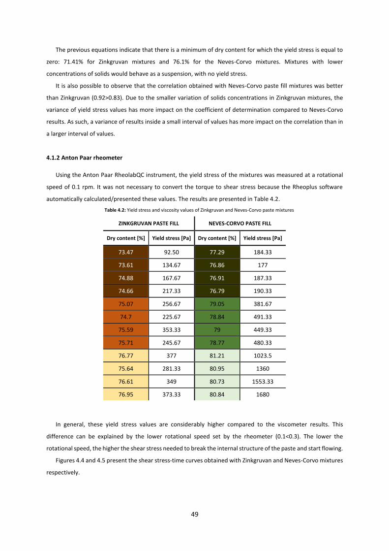
49
The previous equations indicate that there is a minimum of dry content for which the yield stress is equal to
zero: 71.41% for Zinkgruvan mixtures and 76.1% for the Neves-Corvo mixtures. Mixtures with lower
concentrations of solids would behave as a suspension, with no yield stress.
It is also possible to observe that the correlation obtained with Neves-Corvo paste fill mixtures was better
than Zinkgruvan (0.92>0.83). Due to the smaller variation of solids concentrations in Zinkgruvan mixtures, the
variance of yield stress values has more impact on the coefficient of determination compared to Neves-Corvo
results. As such, a variance of results inside a small interval of values has more impact on the correlation than in
a larger interval of values.
4.1.2 Anton Paar rheometer
Using the Anton Paar RheolabQC instrument, the yield stress of the mixtures was measured at a rotational
speed of 0.1 rpm. It was not necessary to convert the torque to shear stress because the Rheoplus software
automatically calculated/presented these values. The results are presented in Table 4.2.
Table 4.2: Yield stress and viscosity values of Zinkgruvan and Neves-Corvo paste mixtures
In general, these yield stress values are considerably higher compared to the viscometer results. This
difference can be explained by the lower rotational speed set by the rheometer (0.1<0.3). The lower the
rotational speed, the higher the shear stress needed to break the internal structure of the paste and start flowing.
Figures 4.4 and 4.5 present the shear stress-time curves obtained with Zinkgruvan and Neves-Corvo mixtures
respectively.
ZINKGRUVAN PASTE FILL NEVES-CORVO PASTE FILL
Dry content [%] Yield stress [Pa] Dry content [%] Yield stress [Pa]
73.47 92.50 77.29 184.33
73.61 134.67 76.86 177
74.88 167.67 76.91 187.33
74.66 217.33 76.79 190.33
75.07 256.67 79.05 381.67
74.7 225.67 78.84 491.33
75.59 353.33 79 449.33
75.71 245.67 78.77 480.33
76.77 377 81.21 1023.5
75.64 281.33 80.95 1360
76.61 349 80.73 1553.33
76.95 373.33 80.84 1680

50
Figure 4.4: Shear stress-time curves for Zinkgruvan paste fill mixtures as recorded by the rheometer
Figure 4.5: Shear stress-time curves for Neves-Corvo paste fill mixtures as recorded by the rheometer
The three domains of each mix design are perceptible in both mine curves, with Zinkgruvan showing some
variance at the curve’s peak. Another noteworthy aspect is the residual shear stress of the curves. The fact that
the curves exhibit intervals of residual shear stress has already been noted. However, in Figure 4.4 is possible to
observe that the curves, after yielding, recover some of the stress and, therefore, the residuals are not distributed
by domains/intervals as shown in Somincor curves. This suggests that Zinkgruvan paste fill could be time-
dependent for shearing at low shear rates (most probably thixotropic behaviour). However, more tests should
be done to prove and understand this rheological behaviour.
The correlation of these yield stress values with the dry content of the mixtures is shown in Figure 4.6.
0
50
100
150
200
250
300
350
400
450
0 50 100 150 200 250
Shea
r St
ress
[P
a]
Time [s]
0
200
400
600
800
1000
1200
1400
1600
1800
0 50 100 150 200 250
Shea
r St
ress
[P
a]
Time [s]

51
Figure 4.6: Correlation graph of yield stress (measured by the rheometer) versus dry content of mixtures
The correlation obtained for both mine mixtures also shows a linear feature. Equations 4.3 and 4.4 define the
yield stress (𝜏𝑟ℎ𝑒𝑜) as a function of dry content (𝐷𝑐) for Zinkgruvan and Neves-Corvo mixtures.
𝐷𝑐 = 0.0105𝜏𝑟ℎ𝑒𝑜 + 72.597 4.3
𝐷𝑐 = 0.0026𝜏𝑟ℎ𝑒𝑜 + 77.113 4.4
The equations indicate that the minimum concentration of solids at which the yield stress is zero is slightly
higher (about 1%) than that previously obtained with the viscometer readings. The R2 values show that the
correlations obtained with both mine mixtures were very close to each other (0.7978≈0.7853), but inferior
compared to the viscometer ones.
In this case, the dry content is not the only variable responsible for the variance of yield stresses. For similar
dry contents, the yield stress results are very different between the two mine mixtures. Several aspects may
explain and contribute to this phenomenon, related to the precision of the equipment and the physical
characteristics of both tailings.
As explained in the State of the Art chapter, yield stress is the critical shear stress that must be exceeded
before irreversible deformation and flow can occur, being associated with the alignment of particles and/or flocs
in the mixture matrix. Associated with the lower rotational speed of the rheometer, the stress needed to move
the particles is higher when compared to higher speed (viscometer). It is possible to observe that for
equal/similar dry contents (Figure 4.6 and Table 4.2) the yield stress of Zinkgruvan mixtures is higher than Neves-
Corvo mixtures. This is the result of the dimensions and geometry of Zinkgruvan tailings particles. Zinkgruvan
tailings are coarser than Neves-Corvo tailing, so the specific surface is smaller, providing less space for particle
movement and less water retention, which can reduce friction between particles. Furthermore, Figure 3.3 shows
that Zinkgruvan tailings are also more angular and elongated than Neves-Corvo tailings, thereby hindering
particle alignment.
Associated with this, it is also important to state that the consistency of results obtained with this equipment
is not as good as with the viscometer. This can be explained by the higher precision of the equipment, making it
susceptible to slight deviations of the vane spindle from the centre of the container, to existent air bubbles, small
agglomerations of particles, wall slip and others. As the container utilised for these measurements was small in
R² = 0.7955
R² = 0.7853
72
73
74
75
76
77
78
79
80
81
82
83
0.00 500.00 1000.00 1500.00 2000.00
Dry
Co
nte
nt
[%]
Yield Stress [Pa]

52
comparison with the dimensions of the vane spindle (Figure 4.7), the slightest deviation of the spindle from the
middle of the container will produce some variance in the results measured.
Figure 4.7: Rheometer vane spindle and container
4.2 Slump
The slump test results are presented with the dry content of the mixtures in Table 4.3.
Table 4.3: Slump values of Zinkgruvan and Neves-Corvo paste mixtures
To better visualise the difference between the slump heights and the appearance of both mine mixtures,
Figure 4.8 shows some photography from the tests.
ZINKGRUVAN PASTE FILL NEVES-CORVO PASTE FILL
Dry content [%] Slump [cm] Dry content [%] Slump [cm]
73.47 11.4 77.29 12.17
73.61 10.93 76.86 12
74.88 9.5 76.91 11.83
74.66 9.5 76.79 12.5
75.07 8.4 79.05 9.5
74.7 7.33 78.84 8.83
75.59 6.67 79 8.33
75.71 6.77 78.77 10.33
76.77 5.43 81.21 4.75
75.64 6.67 80.95 5
76.61 5.9 80.73 4.33
76.95 5.93 80.84 4.5

53
Figure 4.8: Photographic record of slump tests
To correlate these slump values with the dry content of each mixture, Figure 4.9 presents the chart with the
R2 of each correlation.
Figure 4.9: Correlation graph of dry content of mixtures versus slump
These linear correlations are expressed by Equations 4.5 and 4.6 for Zinkgruvan and Neves-Corvo mixtures.
𝐷𝑐 = −0.5𝑠ℎ + 79.29 4.5
𝐷𝑐 = −0.49𝑠ℎ + 83.24 4.6
Equations 4.5 and 4.6 indicate the maximum concentration of solids possible for testing, in these conditions,
which are 79.29% and 83.24% for Zinkgruvan and Neves-Corvo mixtures, respectively.
Observing Table 4.3 and Figure 4.9, it is possible to identify an interval of dry content values (76-78%) for
which the slump heights of Neves-Corvo and Zinkgruvan mixtures are different. Reviewing the State of the Art
chapter, the slump height is an empirical measure of consistency, dependent on both material yield stress and
density. The drop of the material is a result of the shear stress produced by a pressure applied to the top surface
R² = 0.8144
R² = 0.9305
72
73
74
75
76
77
78
79
80
81
82
3 5 7 9 11 13 15
Dry
Co
nte
nt
[%]
Slump height [cm]
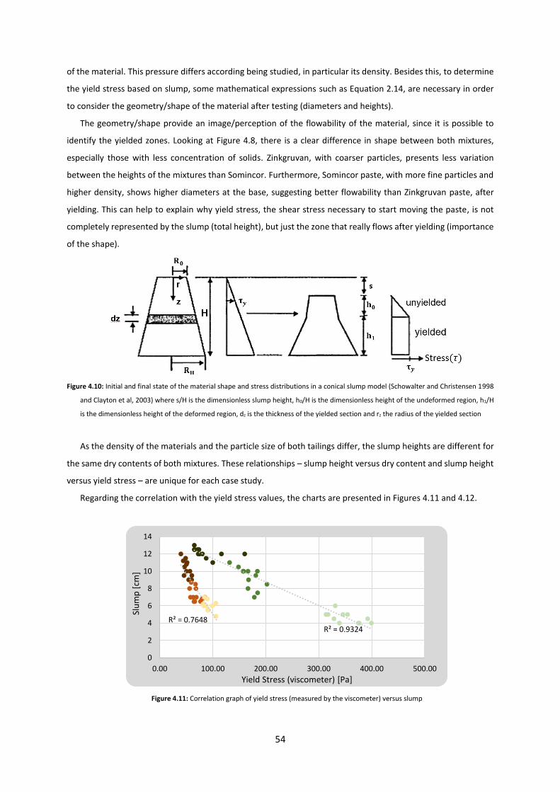
54
of the material. This pressure differs according being studied, in particular its density. Besides this, to determine
the yield stress based on slump, some mathematical expressions such as Equation 2.14, are necessary in order
to consider the geometry/shape of the material after testing (diameters and heights).
The geometry/shape provide an image/perception of the flowability of the material, since it is possible to
identify the yielded zones. Looking at Figure 4.8, there is a clear difference in shape between both mixtures,
especially those with less concentration of solids. Zinkgruvan, with coarser particles, presents less variation
between the heights of the mixtures than Somincor. Furthermore, Somincor paste, with more fine particles and
higher density, shows higher diameters at the base, suggesting better flowability than Zinkgruvan paste, after
yielding. This can help to explain why yield stress, the shear stress necessary to start moving the paste, is not
completely represented by the slump (total height), but just the zone that really flows after yielding (importance
of the shape).
Figure 4.10: Initial and final state of the material shape and stress distributions in a conical slump model (Schowalter and Christensen 1998
and Clayton et al, 2003) where s/H is the dimensionless slump height, h0/H is the dimensionless height of the undeformed region, h1/H
is the dimensionless height of the deformed region, dz is the thickness of the yielded section and rz the radius of the yielded section
As the density of the materials and the particle size of both tailings differ, the slump heights are different for
the same dry contents of both mixtures. These relationships – slump height versus dry content and slump height
versus yield stress – are unique for each case study.
Regarding the correlation with the yield stress values, the charts are presented in Figures 4.11 and 4.12.
Figure 4.11: Correlation graph of yield stress (measured by the viscometer) versus slump
R² = 0.7648R² = 0.9324
0
2
4
6
8
10
12
14
0.00 100.00 200.00 300.00 400.00 500.00
Slu
mp
[cm
]
Yield Stress (viscometer) [Pa]

55
The correlations presented in the above chart are expressed by linear equations 4.7 and 4.8 for Zinkgruvan
and Neves-Corvo mixtures respectively.
𝑠ℎ = −0.095𝜏𝑣𝑖𝑠𝑐 + 14.53 4.7
𝑠ℎ = −0.027𝜏𝑣𝑖𝑠𝑐 + 14.17 4.8
These equations indicate that there is a maximum slump height for which the yield stress, measured by the
viscometer, is zero. Both maximum slump heights, 14.53 cm and 14.17 cm, are really close to the height of
slump mould (15 cm). This represents a very good correspondence between the yield stress values measured
by the viscometer at 0.3 rpm with the mini slump cone test.
Figure 4.12: Correlation graph of yield stress (measured by the rheometer) versus slump
The correlations presented in the above chart are expressed by linear equations 4.9 and 4.10 for Zinkgruvan
and Neves-Corvo mixtures respectively.
𝑠ℎ = −0.019𝜏𝑟ℎ𝑒𝑜 + 12.65 4.9
𝑠ℎ = −0.0053𝜏𝑟ℎ𝑒𝑜 + 12.35 4.10
In this case, the maximum slump heights are lower than the previous, but also very close to each other. The
explanation for this may be related to the dry content of the mixtures. Previously, the correlation between the
yield stress measured by both equipment and the dry content of mixtures has shown different minimum dry
contents for which the yield stress would be zero. For rheometer results, this minimum dry content is higher
than viscometer data for both mine tailings (71.41% < 72.59% and 76.1% < 77.1%). Therefore, mixtures with a
higher concentration of solids occupy more volume and so the slump height should be higher.
R² = 0.7843
R² = 0.8555
0
2
4
6
8
10
12
14
0.00 500.00 1000.00 1500.00 2000.00
Slu
mp
[cm
]
Yield Stress (rheometer) [Pa]

56
4.3 Flow table
The flow table results, including the initial and final diameters, of all mixtures are shown in Table 4.4.
Table 4.4: Flow table values of Zinkgruvan and Neves-Corvo paste mixtures
It is evident that for higher values of dry content, the initial diameters are pretty close to each other (≈9.5
cm), corresponding to the diameter of the mould. To better visualise the difference between the flow table
diameters and the appearance of both mine mixtures, Figure 4.13 shows some photography from the tests.
Figure 4.13: Photographic record of flow table tests
To correlate the initial diameter values with the dry content of each mixture, Figure 4.14 presents the chart
with the R2 of each correlation.
ZINKGRUVAN PASTE FILL NEVES-CORVO PASTE FILL
Dry content [%] FTS initial
diameter [cm] FTS final diameter [cm]
Dry content [%]
FTS initial diameter [cm]
FTS final diameter [cm]
73.47 13.17 24.08 77.29 14.33 23.25
73.61 12.17 24.08 76.86 17.83 24.92
74.88 10.58 23.42 76.91 16 23.83
74.66 10.58 22.5 76.79 17.75 25.17
75.07 10.63 22.13 79.05 10.25 20.75
74.7 10.5 22.58 78.84 10 21.17
75.59 9.67 21.67 79 9.92 20.58
75.71 9.58 20.08 78.77 10.75 21.67
76.77 9.75 18 81.21 9.125 16.125
75.64 9.58 19.33 80.95 9.17 17.75
76.61 9.5 18.33 80.73 9.25 17.08
76.95 9.5 17.83 80.84 9.25 18.67

57
Figure 4.14: Correlation graph of dry content of mixtures versus initial diameter of flow table tests
Overall, the data obtained show a linear feature for the range of solid content tested for each mine. The
following linear equations (4.11 and 4.12), which define the initial diameter of flow table (𝑑𝑖) as a function of dry
content (𝐷𝑐), for Zinkgruvan and Neves-Corvo mixtures respectively, are:
𝑑𝑖 = −0.9𝐷𝑐 + 78.51 4.11
𝑑𝑖 = −1.9𝐷𝑐 + 161.6 4.12
The correlation with the yield stress values is presented in Figures 4.15 and 4.16 and the equations of trend
lines.
Figure 4.15: Correlation graph of yield stress (measured by the viscometer) versus initial diameter of flow table tests
R² = 0.7432R² = 0.8002
6
8
10
12
14
16
18
20
72 74 76 78 80 82
Init
ial D
iam
eter
[cm
]
Dry Content [%]
𝑑𝑖 = -0.05𝜏𝑣𝑖𝑠𝑐 + 13.84R² = 0.5785
𝑑𝑖 = -0.024𝜏𝑣𝑖𝑠𝑐 + 16.89R² = 0.6318
0
2
4
6
8
10
12
14
16
18
20
0.00 100.00 200.00 300.00 400.00 500.00
Init
ial D
iam
eter
[cm
]
Yield Stress (viscometer) [Pa]

58
Figure 4.16: Correlation graph of yield stress (measured by the rheometer) versus initial diameter of flow table tests
Looking at both graphs, the behaviour of trend lines is the same but with different intervals of action.
However, what was noticed in Table 4.4 is now confirmed. For higher yield stress values, the initial diameters are
too equal, forming a horizontal line that corresponds to the diameter of the cone mould. From the results
obtained, it is possible to conclude that this method is not able to provide a proper evaluation of paste fill with
a high concentration of solids, which is the main goal of this technology.
In relation to the results of the final diameter of flow table, the correlation with the dry content of mixtures
is presented in Figure 4.17.
Figure 4.17: Correlation graph of dry content of mixtures versus final diameter of flow table tests
The data obtained shows a linear feature for the range of dry content tested for each mine. The linear
equations, which define the dry content (𝐷𝑐) as a function of final diameter of flow table (𝑑𝑓), for Zinkgruvan and
Neves-Corvo mixtures respectively, are as follows:
𝐷𝑐 = −0.45𝑑𝑓 + 84.85 4.17
𝐷𝑐 = −0.55𝑑𝑓 + 90.45 4.18
𝑑f = -0.01𝜏rheo + 13R² = 0.6379 𝑑f = -0.0043𝜏rheo + 14.9
R² = 0.4585
0
2
4
6
8
10
12
14
16
18
20
0.00 500.00 1000.00 1500.00 2000.00
Init
ial D
iam
eter
[cm
]
Yield Stress (rheometer) [Pa]
R² = 0.8847
R² = 0.9473
72
73
74
75
76
77
78
79
80
81
82
83
15 17 19 21 23 25 27
Dry
Co
nte
nt
[%]
Final diameter [cm]
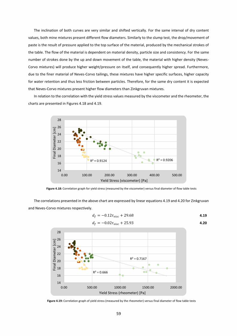
59
The inclination of both curves are very similar and shifted vertically. For the same interval of dry content
values, both mine mixtures present different flow diameters. Similarly to the slump test, the drop/movement of
paste is the result of pressure applied to the top surface of the material, produced by the mechanical strokes of
the table. The flow of the material is dependent on material density, particle size and consistency. For the same
number of strokes done by the up and down movement of the table, the material with higher density (Neves-
Corvo mixtures) will produce higher weight/pressure on itself, and consequently higher spread. Furthermore,
due to the finer material of Neves-Corvo tailings, these mixtures have higher specific surfaces, higher capacity
for water retention and thus less friction between particles. Therefore, for the same dry content it is expected
that Neves-Corvo mixtures present higher flow diameters than Zinkgruvan mixtures.
In relation to the correlation with the yield stress values measured by the viscometer and the rheometer, the
charts are presented in Figures 4.18 and 4.19.
Figure 4.18: Correlation graph for yield stress (measured by the viscometer) versus final diameter of flow table tests
The correlations presented in the above chart are expressed by linear equations 4.19 and 4.20 for Zinkgruvan
and Neves-Corvo mixtures respectively.
𝑑𝑓 = −0.12𝜏𝑣𝑖𝑠𝑐 + 29.68 4.19
𝑑𝑓 = −0.02𝜏𝑣𝑖𝑠𝑐 + 25.93 4.20
Figure 4.19: Correlation graph of yield stress (measured by the rheometer) versus final diameter of flow table tests
R² = 0.9124 R² = 0.9206
14
16
18
20
22
24
26
28
0.00 100.00 200.00 300.00 400.00 500.00
Fin
al D
iam
eter
[cm
]
Yield Stress (viscometer) [Pa]
R² = 0.666
R² = 0.7167
14
16
18
20
22
24
26
28
0.00 500.00 1000.00 1500.00 2000.00
Fin
al D
iam
eter
[cm
]
Yield Stress (rheometer) [Pa]
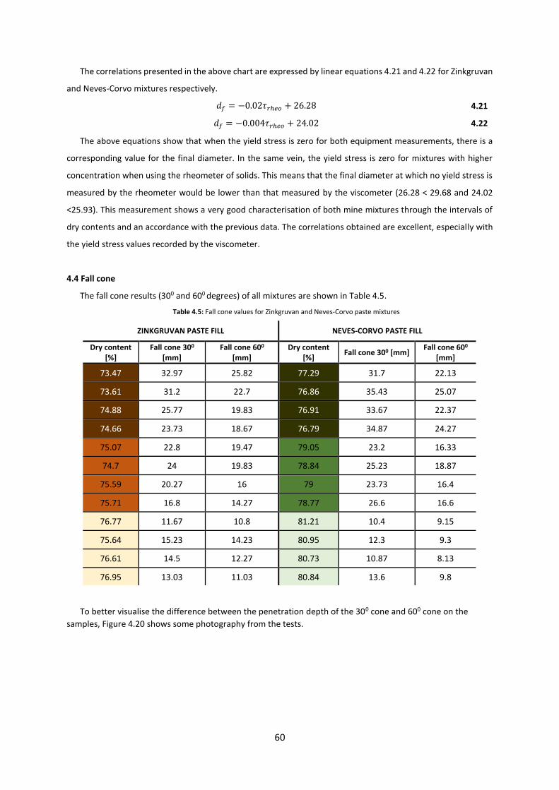
60
The correlations presented in the above chart are expressed by linear equations 4.21 and 4.22 for Zinkgruvan
and Neves-Corvo mixtures respectively.
𝑑𝑓 = −0.02𝜏𝑟ℎ𝑒𝑜 + 26.28 4.21
𝑑𝑓 = −0.004𝜏𝑟ℎ𝑒𝑜 + 24.02 4.22
The above equations show that when the yield stress is zero for both equipment measurements, there is a
corresponding value for the final diameter. In the same vein, the yield stress is zero for mixtures with higher
concentration when using the rheometer of solids. This means that the final diameter at which no yield stress is
measured by the rheometer would be lower than that measured by the viscometer (26.28 < 29.68 and 24.02
<25.93). This measurement shows a very good characterisation of both mine mixtures through the intervals of
dry contents and an accordance with the previous data. The correlations obtained are excellent, especially with
the yield stress values recorded by the viscometer.
4.4 Fall cone
The fall cone results (300 and 600 degrees) of all mixtures are shown in Table 4.5.
Table 4.5: Fall cone values for Zinkgruvan and Neves-Corvo paste mixtures
To better visualise the difference between the penetration depth of the 300 cone and 600 cone on the
samples, Figure 4.20 shows some photography from the tests.
ZINKGRUVAN PASTE FILL NEVES-CORVO PASTE FILL
Dry content [%]
Fall cone 300 [mm]
Fall cone 600 [mm]
Dry content [%]
Fall cone 300 [mm] Fall cone 600
[mm]
73.47 32.97 25.82 77.29 31.7 22.13
73.61 31.2 22.7 76.86 35.43 25.07
74.88 25.77 19.83 76.91 33.67 22.37
74.66 23.73 18.67 76.79 34.87 24.27
75.07 22.8 19.47 79.05 23.2 16.33
74.7 24 19.83 78.84 25.23 18.87
75.59 20.27 16 79 23.73 16.4
75.71 16.8 14.27 78.77 26.6 16.6
76.77 11.67 10.8 81.21 10.4 9.15
75.64 15.23 14.23 80.95 12.3 9.3
76.61 14.5 12.27 80.73 10.87 8.13
76.95 13.03 11.03 80.84 13.6 9.8
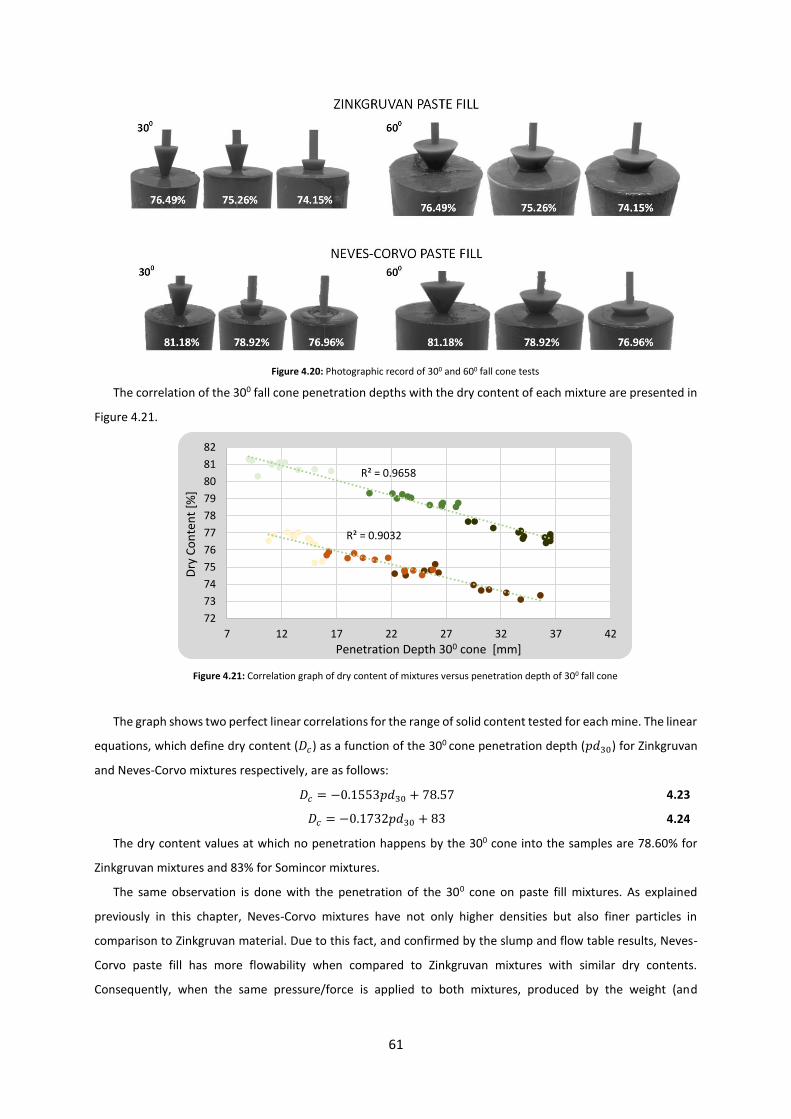
61
Figure 4.20: Photographic record of 300 and 600 fall cone tests
The correlation of the 300 fall cone penetration depths with the dry content of each mixture are presented in
Figure 4.21.
Figure 4.21: Correlation graph of dry content of mixtures versus penetration depth of 300 fall cone
The graph shows two perfect linear correlations for the range of solid content tested for each mine. The linear
equations, which define dry content (𝐷𝑐) as a function of the 300 cone penetration depth (𝑝𝑑30) for Zinkgruvan
and Neves-Corvo mixtures respectively, are as follows:
𝐷𝑐 = −0.1553𝑝𝑑30 + 78.57 4.23
𝐷𝑐 = −0.1732𝑝𝑑30 + 83 4.24
The dry content values at which no penetration happens by the 300 cone into the samples are 78.60% for
Zinkgruvan mixtures and 83% for Somincor mixtures.
The same observation is done with the penetration of the 300 cone on paste fill mixtures. As explained
previously in this chapter, Neves-Corvo mixtures have not only higher densities but also finer particles in
comparison to Zinkgruvan material. Due to this fact, and confirmed by the slump and flow table results, Neves-
Corvo paste fill has more flowability when compared to Zinkgruvan mixtures with similar dry contents.
Consequently, when the same pressure/force is applied to both mixtures, produced by the weight (and
R² = 0.9032
R² = 0.9658
72
73
74
75
76
77
78
79
80
81
82
7 12 17 22 27 32 37 42
Dry
Co
nte
nt
[%]
Penetration Depth 300 cone [mm]

62
geometry) of the cone, the penetration depth will be higher in Neves-Corvo mixtures. The same is true of the 600
cone.
The correlation between the 300 fall cone results and the yield stress values measured by the viscometer and
the rheometer are presented in Figures 4.22 and 4.23.
Figure 4.22: Correlation graph for yield stress (measured by the viscometer) versus penetration depth of 300 fall cone
The correlations presented in the above chart are expressed by linear equations 4.25 and 4.26 for Zinkgruvan
and Neves-Corvo mixtures respectively.
𝑝𝑑30 = −0.35𝜏𝑣𝑖𝑠𝑐 + 45.22 4.25
𝑝𝑑30 = −0.08𝜏𝑣𝑖𝑠𝑐 + 39.76 4.26
Figure 4.23: Correlation graph of yield stress (measured by the rheometer) versus penetration depth of 300 fall cone
The correlations presented in the above chart are expressed by linear equations 4.27 and 4.28 for Zinkgruvan
and Neves-Corvo mixtures respectively.
𝑝𝑑30 = −0.063𝜏𝑟ℎ𝑒𝑜 + 37.15 4.27
𝑝𝑑30 = −0.015𝜏𝑟ℎ𝑒𝑜 + 33.95 4.28
The above equations indicate that there is a certain penetration depth at which the yield stress is equal to
zero. The correlations obtained are very good, especially with the viscometer results concerning R2 values.
R² = 0.8593 R² = 0.9537
0
5
10
15
20
25
30
35
40
0.00 100.00 200.00 300.00 400.00 500.00
Pen
etra
tio
n D
epth
30
0co
ne
[m
m]
Yield Stress (viscometer) [Pa]
R² = 0.7551
R² = 0.805
0
5
10
15
20
25
30
35
40
0.00 500.00 1000.00 1500.00 2000.00
Pen
etra
tio
n D
epth
30
0co
ne
[mm
]
Yield Stress (rheometer) [Pa]

63
The correlation between the 600 fall cone penetration depths and the dry content of each mixture is
presented in Figure 4.24.
Figure 4.24: Correlation graph for dry content of mixtures versus penetration depth of 600 fall cone
As before, the graph shows two linear features for the range of solid content tested for each mine. The linear
equations, which define the dry content (𝐷𝑐) as a function of the 600 cone penetration depth (𝑝𝑑60), for
Zinkgruvan and Neves-Corvo mixtures respectively, are as follows:
𝐷𝑐 = −0.22𝑝𝑑60 + 79 4.29
𝐷𝑐 = −0.26𝑝𝑑60 + 83.17 4.30
The dry content values at which the 600 cone does not penetrate into the samples are 79% for Zinkgruvan
mixtures and 83.17% for Somincor mixtures, the same as for the 300 cone. It is possible to observe more
dispersion of results compared to the previous cone geometry.
The correlation between the 600 fall cone results and the yield stress values measured by the viscometer and
the rheometer is presented in Figures 4.25 and 4.26.
Figure 4.25: Correlation graph for yield stress (measured by the viscometer) versus penetration depth of 600 fall cone
The correlations presented in the above chart are expressed by linear equations 4.31 and 4.32 for Zinkgruvan
and Neves-Corvo mixtures respectively.
R² = 0.8497
R² = 0.9289
72
73
74
75
76
77
78
79
80
81
82
5 10 15 20 25 30
Dry
Co
nte
nt
[%]
Penetration Depth 600 cone [mm]
R² = 0.808
R² = 0.9104
0
5
10
15
20
25
30
0.00 100.00 200.00 300.00 400.00 500.00
Pen
etra
tio
n D
epth
60
0co
ne
[mm
]
Yield Stress (viscometer) [Pa]

64
𝑝𝑑60 = −0.23𝜏𝑣𝑖𝑠𝑐 + 33.45 4.31
𝑝𝑑60 = −0.05𝜏𝑣𝑖𝑠𝑐 + 27 4.32
Figure 4.26: Correlation graph of yield stress (measured by the rheometer) versus penetration depth of 600 fall cone
The correlations presented in the above chart are expressed by linear equations 4.33 and 4.34 for Zinkgruvan
and Neves-Corvo mixtures respectively.
𝑝𝑑60 = −0.042𝜏𝑟ℎ𝑒𝑜 + 28.04 4.33
𝑝𝑑60 = −0.0099𝜏𝑟ℎ𝑒𝑜 + 23.35 4.34
Following on from the previous data, these equations indicate the penetration depth at which the yield stress
is equal to zero for both mixtures. Due to the dispersion of yield stress values measured by the rheometer, the
correlations are not as good as the previous ones.
Not only did the fall cone results provide a very good characterisation of both mine mixtures through the
intervals of dry contents chosen and the correlation with the yield stress values measured, but they were also
the method with the best performance.
4.5 Data analysis
From the data presented, there are important aspects that must be analysed and explained/justified in order
to draw a conclusion about the quality and precision of all of the experimental work that has been carried out.
When observing the tables in Annexes I and II, the first thing that becomes evident is the difference between
the solid content calculated for the mix design and the dry content measured after mixing, which should be the
same. This difference is more obvious with the Zinkgruvan mixtures (about 4%). There is not a single reason that
explains this variance. Errors associated with the determination of water content of the tailings and dry content
of the mixtures may have an influence, as just a small sample was weighed for both measurements, so the
quantity of the weighed samples could not represent the entire mixture/tailings. Furthermore, the mineralogy
of both tailings is different, and so is the percentage of water present inside the particles. Due to the temperature
and time setup for evaporation, this water could not be released. Nevertheless, the dry content values are
R² = 0.7166
R² = 0.7878
0
5
10
15
20
25
30
0.00 500.00 1000.00 1500.00 2000.00
Pen
etra
tio
n D
epth
60
0co
ne
[m
m]
Yield Stress (rheometer) [Pa]

65
consistent for each mix design. The sampling process, which involved dividing the tailings from each barrel and
putting them in individual bags, led to better control of each sample and provided more consistent data.
The mix designs set for each mine tailings, during the initial run practice, were different in terms of workability
range. The interval of solid content was set consonant with the interval where the mixtures behave as a paste
and not as a soil or a suspension. This range was smaller for Zinkgruvan mixtures (78–80% and 79–81%) than for
Neves-Corvo mixtures (78%–82%), mainly due to the physical properties of both tailings. By overlaying the PSD
of each mine tailings with Figure 2.13, which represents the Canadian hard rock mine tailings PSD curves
envelope, it is clear that Zinkgruvan tailings are coarser than Neves-Corvo tailings and present a steeper curve,
creating a sharper transition between particle sizes (Figure 4.27).
Figure 4.27: Overlaying of the PSD curves of Zinkgruvan (orange) and Neves-Corvo tailings (yellow) on the Canadian hard rock mine
tailings PSD curves envelope
In general, if all else is equal, finer slurries generally display a more gradual increase in yield stress with
increasing solids concentration, whereas coarse materials show a relatively sharp transition from liquid-like to
solid-like behaviour (Sofra, 2017), which may justify the smaller interval of workability for Zinkgruvan paste fill
when compared with a finer material such Neves-Corvo tailings, using the same cement percentage and water.
In addition to this, as observed in Chapter 3, there is a slight variation in the Zinkgruvan tailings’ PSD curves,
suggesting different times of sampling. This fact was confirmed during the practice run, as two different intervals
of solid content (78–80% and 79–81%) were set for barrels 1 and 2 and barrels 3 and 4. However, these
differences were not noticeable with the results and time-curve behaviours obtained with the viscometer and
rheometer, proving that there was not any type of interference due to the difference of sampling. The
adjustment made with the mix designs was enough to normalise the samples. This is a practical example of
tailings changeability (variations of ore bodies, state of weathering of the sample, water quality, etc.), making
sample selection very important issue for rheological studies.
Another aspect that is noticeable in Annexes I and II is the difference between the densities of both paste
mixtures, which can be explained by the increase of solids concentration of the mixtures but, essentially, because

66
of the mineralogy of the tailings. Neves-Corvo tailings contain denser elements (Fe2O3, SO3, etc.) than Zinkgruvan
tailings (SiO2, Al2O3, etc.).
The determination of the yield stress is the most fundamental and important rheological parameter for the
design and operation of a paste system (Sofra, 2017). As discussed before in Chapter 3, the way this property is
measured is of most importance because, when performed correctly, the yield stress gives the best indication of
the magnitude of the effects of physical, chemical mineralogical, shear and time variables on the overall
rheological properties of the paste, and should be the starting point for any rheological testing programme
(Sofra, 2017). In this regard, the yield stress of all mixtures was determined by the vane technique, widely
accepted by many authors as the best method for achieving the “true” yield stress: “the great advantage of the
vane is the material yields on itself (…) this technique is now used worldwide for measurement of yielding in all
matter of materials and was motivated by the need to understand the true yielding behaviour under plant/site
conditions” (Sofra, 2017). This technique can be applied to a viscometer or a rheometer, depending on the
availability of equipment, making a difference to the slower rotational speed capacity of the rheometers.
Therefore, equipment with different rotational speeds (0.1 and 0.3 rpm) was utilised in order to better
understand and evaluate the differences of yield stress values obtained. The results obtained were analysed and
correlated with the other test methods to evaluate their adjustment to the data.
In terms of the yield stress values obtained, those gauged with the rheometer were, as expected, higher.
However, the consistency of the results was not so good in comparison with the values measured by the
viscometer. This can be explained by the higher precision of the equipment, making it particularly susceptible to
slight deviations of the vane spindle from the centre of the container, to existent air bubbles, small
agglomerations of particles, wall slip and other factors. Another aspect is related to the dimensions of the
container utilised for these measurements: the distance from the vane spindle to the edge of the container was
too small. Previous projects that involved using a vane in a cup to minimise slip (Barnes and Carnalli, 1990) and
infinite medium analysis (Kreiger and Maron, 1954) have proven the major advantages of using the vane in an
infinite medium for this type of measurement, such as (Sofra, 2017): insertion of a vane causes less sample
disturbance, minimising thixotropic breakdown; the vane in cup is less susceptible to errors arising from large
particle sizes; yielding occurs between layers of fluid; minimising the effects of wall slip, and others. Since
Zinkgruvan tailings are coarser than Neves-Corvo material, the presence of large particles and more air voids
causes more disturbance during the rotation of the vane spindle. That is the reason that the results from
Zinkgruvan are not as consistent as those from Neves-Corvo.
Due to the higher rotational speed of the viscometer, the values of yield stress are smaller. The dimensions
of the container were high enough compared to the diameter of the vane spindle, creating an infinite medium
for measuring paste rheology. The problems associated with this issue were thus eliminated. Both mine mixtures
presented consistent results and behaviours.
In general, it is worth noting that Neves-Corvo mixtures present higher yield stress values in comparison with
Zinkgruvan mixtures for the same solids concentration. This can also be explained by the physical and chemical
differences of both tailings. Using the same principle, if all else is equal, a finer grind material will have a higher
yield stress and viscosity at a given solids concentration due to the finer slurry having a greater particle-specific

67
surface area and therefore a greater area available for interparticle interactions (Sofra, 2017). In terms of the
influence of tailings mineralogy on rheological properties of paste fill, only general information is available in
academic works. Therefore, is difficult to say conclusively what parameters, in this case, most affect the rheology
of paste backfill in terms of chemical composition. In general, as Neves-Corvo mixtures are denser than those
from Zinkgruvan, due to their mineralogy, the shear necessary to start flowing is naturally, higher.
The test methods applied in this experimental work are well known in the mining industry for evaluating the
rheology of concrete/paste backfill, particularly the slump test. There are formulations that allow us to determine
the yield stress and viscosity of the samples from the results of these tests, as presented in Chapter 2. However,
the objective of this work was to evaluate the fitting capacity of these methodologies to different paste fill
mixtures, with different tailings and mix designs, and to determine the veracity and quality of the results and the
correlations with the yield stress values measured by a rheometer and a viscometer. The relationship between
data is very important to really understand the uniqueness of each case of study.
Overall, the measurement that presented the worst performance was the initial diameter of flow table. As
explained before, this measure is not able to characterise mixtures with higher dry contents, keeping the same
diameter as the cone mould. Apart from this, all of the methods were able to evaluate difference mix designs
and obtain good correlations with the yield stress values. Table 4.6 shows the coefficients of determination (R2)
of all correlations previously determined.
Table 4.6: Coefficient of determination values of test methods versus the dry content of mixtures and the yield stress values measured
by viscometer and rheometer equipment (orange – Zinkgruvan mixtures; green – Neves-Corvo mixtures)
Slump FT final diameter 300 Cone 600 Cone
Dry Content 0.8144 0.8847 0.9032 0.8497
0.9305 0.9473 0.9658 0.9289
YS (viscometer) 0.7648 0.9124 0.8593 0.808
0.9324 0.9206 0.9537 0.9104
YS (rheometer) 0.7843 0.666 0.7551 0.7166
0.8555 0.7167 0.805 0.7878
Slump test is a simple method of measuring the yield stress and is widely used for quality control or rapid on-
site measurements. However, slump heights cannot be generalised between contexts, as a slump value
corresponds a certain yield stress, specific to just one material/sample. This is confirmed by the differences in
the yield stress values obtained from Zinkgruvan and Neves-Corvo mixtures for the same slump height, as
observed in Figure 4.9. The solid concentration versus slump relationship is unique to each material, and so are
the corresponding yield stress values. The data obtained proved that the mini slump cone used fits very well with
the viscometer yield stress values.
The flow table used is often applied to the study of cement mortar. The final diameter proved to be a very
good measurement of paste fill rheology. The data was consistent and the correlations with the yield stress
values were even better in comparison to the slump test.
Finally, the adapted fall cone test turned out to be the methodology that performed best, with very good
correlation with dry content of the mixtures and with the yield stress values achieved by the viscometer and

68
rheometer. The weight and geometry of the cones combined with the time released proved to be a successful
procedure for measuring paste fill rheology, and is one of this work’s major contributions. This equipment can
become a simple, inexpensive, convenient and fast method of determining the yield stress, ideal for quality
control or rapid on-site measurements.
4.6 Data modelling
The results obtained with the viscometer and the rheometer, using the vane technique, showed that the
yield stress range for Zinkgruvan and Somincor mixtures was different. Various explanations were put forward
for this, starting with the different rotational speeds of both pieces of equipment. Furthermore, it was found that
different variables/parameters influenced both yield stresses. In the case of the viscometer measurements, at
0.3rpm, the dry content of mixtures appeared to be the main variable that affected this rheological property. On
the other hand, for the rheometer set at 0.1rpm, the physical characteristics of tailings were important as well
as the dry content.
To confirm, mathematically, these assumptions, two detailed statistical studies were developed. These
are based on the proposal and validation of multiple linear regression models to predict yield stresses measured
by both pieces of equipment (dependent variable) of all mixtures, as a function of quantitative predictors,
obtained by the experimental work.
The quantitative predictors are dry content and particle size distribution characteristics of both tailings
(obtained from table 3.7), namely, the percentage of material passing under 20 𝜇𝑚, the uniformity coefficient
(𝐶𝑢) and the coefficient of gradation (𝐶𝑐). The remaining characteristic diameters were not considered because
they are applied in the calculation of coefficients 𝐶𝑢 and 𝐶𝑐.
Consequently, the mathematical relation between the predictors (quantitative explanatory variables) and the
dependent variables can be generically defined by Equations 4.35 and 4.36:
𝑌𝑖𝑒𝑙𝑑 𝑠𝑡𝑟𝑒𝑠𝑠𝑣𝑖𝑠𝑐 = 𝑓(𝑑𝑟𝑦𝐶, < 20𝜇𝑚, 𝐶𝑐, 𝐶𝑢) 4.35
𝑌𝑖𝑒𝑙𝑑 𝑠𝑡𝑟𝑒𝑠𝑠𝑟ℎ𝑒𝑜 = 𝑓(𝑑𝑟𝑦𝐶, < 20𝜇𝑚, 𝐶𝑐 , 𝐶𝑢) 4.36
For the determination of each model, the correspondent explanatory variables are represented by a
rectangular matrix 𝐗, of size 𝑛 × 𝑘. Each row of the matrix represents an observation. The number of columns,
𝑘, of the matrix is equal to the sum of the number of quantitative predictors.
Due to the different domains of each explanatory variable and, consequently, to avoid their numerical
influence on the regression analysis, a zscore normalization (Houcque, 2005) was applied to all variables.
In addition to this, it’s well known (Kutner et al., 2005; Draper and Smith, 1998) that result uniqueness and
quality from estimation exercise for multiple linear regression model parameters determination, by the linear
least square method, is critically dependent on the detection and elimination of collinearities or perfect linear
relations between X matrix columns (linear dependent columns) or strongly correlated columns (absolute value
of the correlation coefficients greater than or equal to 0.99) (Paneiro et al., 2015).
One simple technique, applied in this study, for collinearity detection and elimination, is based on the
construction of a squared matrix 𝑪, 𝑘 × 𝑘, of the correlation coefficients between pairs of columns of matrix 𝐗.

69
Thus, one of the columns from the columns pairs with absolute values greater than 0.99, is removed from matrix
𝐗. Another alternative technique consists on the application of Gauss–Jordan elimination method (Strang, 1988),
with the reduction of matrix 𝐗 to a reduced row echelon form, it identifies linearly independent columns with
the automatic computation of the rank of the matrix 𝐗 (Paneiro et al., 2015).
In general, multiple linear regression models with the original or transformed variables approximate the
Equations 4.35 and 4.36:
𝑦 = 𝛽0 + 𝛽1𝑋1 + 𝛽2𝑋2 + 𝛽3𝑋3 + 𝛽4𝑋4 + 𝜖 4.37
In this study, 𝑦 =yield stress, 𝑋1 = dryC, 𝑋2 =< 20𝜇𝑚, 𝑋3 = 𝐶𝑐, and 𝑋4 = 𝐶𝑢.
Data regression analysis can be made by proposal and validation of multiple linear regression model
variations. A set of eight candidate’s models were submitted for both analysis developed by a MATLAB script.
The following table presents the general expressions for all eight multiple linear regression models considered
for these studies.
Table 4.7: Multiple linear regression models considered in the study
Model General expression
1 𝑦 = 𝛽0 + 𝛽1𝑋1 + 𝛽2𝑋2 + 𝛽3𝑋3 + 𝛽4𝑋4
2 𝑦 = 𝛽1𝑋1 + 𝛽2𝑋2 + 𝛽3𝑋3 + 𝛽4𝑋4
3 log (𝑦) = 𝛽0 + 𝛽1𝑋1 + 𝛽2𝑋2 + 𝛽3𝑋3 + 𝛽4𝑋4
4 log (𝑦) = 𝛽1𝑋1 + 𝛽2𝑋2 + 𝛽3𝑋3 + 𝛽4𝑋4
5 𝑦 = 𝛽0 + 𝛽1log (𝑋1) + 𝛽2𝑙𝑜𝑔(𝑋2) + 𝛽3log (𝑋3) + 𝛽4log (𝑋4)
6 y = 𝛽1log (𝑋1) + 𝛽2𝑙𝑜𝑔(𝑋2) + 𝛽3log (𝑋3) + 𝛽4log (𝑋4)
7 log (𝑦) = 𝛽0 + 𝛽1log (𝑋1) + 𝛽2𝑙𝑜𝑔(𝑋2) + 𝛽3log (𝑋3) + 𝛽4log (𝑋4)
8 log (𝑦) = 𝛽1log (𝑋1) + 𝛽2𝑙𝑜𝑔(𝑋2) + 𝛽3log (𝑋3) + 𝛽4log (𝑋4)
The validation of each candidate model includes the statistical significance of the estimated parameters, the
suitability of the adjusted model by analysis of variance (decomposition of the total sum of squares of the
residuals) and the statistical quality of the regression model through residual analysis (Paneiro et al., 2015). In
this sequence, the models quality was evaluated by the following criteria:
the coefficients of determination (𝑅2 and 𝑅2 𝑎𝑑𝑗𝑢𝑠𝑡𝑒𝑑);
analysis of variance (ANOVA) table;
Akaike and Schwarz-Bayesian information criteria (AIC and SBIC).
The model with best performance on previous points is the best candidate model with high ability for
generalization.
𝐘𝐢𝐞𝐥𝐝 𝐬𝐭𝐫𝐞𝐬𝐬𝒗𝒊𝒔𝒄 STATISTICAL STUDY
The candidate models that show the best coefficients of determination, 𝑅2 and 𝑎𝑑𝑗𝑢𝑠𝑡𝑒𝑑 𝑅2, with the values
greater than 0.90, are models 3 and 7, in which 𝛽0 = 4.6571. The adjusted coefficients of determination of model
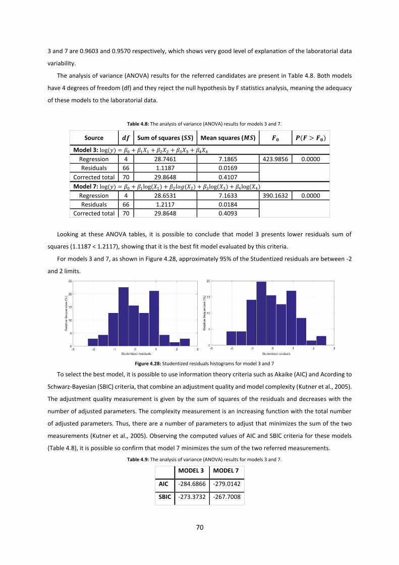
70
3 and 7 are 0.9603 and 0.9570 respectively, which shows very good level of explanation of the laboratorial data
variability.
The analysis of variance (ANOVA) results for the referred candidates are present in Table 4.8. Both models
have 4 degrees of freedom (df) and they reject the null hypothesis by F statistics analysis, meaning the adequacy
of these models to the laboratorial data.
Table 4.8: The analysis of variance (ANOVA) results for models 3 and 7.
Source 𝒅𝒇 Sum of squares (𝑺𝑺) Mean squares (𝑴𝑺) 𝑭𝟎 𝑷(𝑭 > 𝑭𝟎)
Model 3: log (𝑦) = 𝛽0 + 𝛽1𝑋1 + 𝛽2𝑋2 + 𝛽3𝑋3 + 𝛽4𝑋4
Regression 4 28.7461 7.1865 423.9856 0.0000
Residuals 66 1.1187 0.0169
Corrected total 70 29.8648 0.4107
Model 7: log (𝑦) = 𝛽0 + 𝛽1log (𝑋1) + 𝛽2𝑙𝑜𝑔(𝑋2) + 𝛽3log (𝑋3) + 𝛽4log (𝑋4)
Regression 4 28.6531 7.1633 390.1632 0.0000
Residuals 66 1.2117 0.0184
Corrected total 70 29.8648 0.4093
Looking at these ANOVA tables, it is possible to conclude that model 3 presents lower residuals sum of
squares (1.1187 < 1.2117), showing that it is the best fit model evaluated by this criteria.
For models 3 and 7, as shown in Figure 4.28, approximately 95% of the Studentized residuals are between -2
and 2 limits.
Figure 4.28: Studentized residuals histograms for model 3 and 7
To select the best model, it is possible to use information theory criteria such as Akaike (AIC) and Acording to
Schwarz-Bayesian (SBIC) criteria, that combine an adjustment quality and model complexity (Kutner et al., 2005).
The adjustment quality measurement is given by the sum of squares of the residuals and decreases with the
number of adjusted parameters. The complexity measurement is an increasing function with the total number
of adjusted parameters. Thus, there are a number of parameters to adjust that minimizes the sum of the two
measurements (Kutner et al., 2005). Observing the computed values of AIC and SBIC criteria for these models
(Table 4.8), it is possible so confirm that model 7 minimizes the sum of the two referred measurements.
Table 4.9: The analysis of variance (ANOVA) results for models 3 and 7.
MODEL 3 MODEL 7
AIC -284.6866 -279.0142
SBIC -273.3732 -267.7008

71
In this sequence, model 7 is the best-fit model, from the eight candidate models, that satisfies all considered
statistical analysis criteria. In order to write the general model, a statistical significance analysis of the regression
model parameters is made (Kutner et al., 2005). Table 4.10 summarize the results for the estimation exercise of
p parameters, including: Estimated values of the estimated model parameters: 𝛽�̂�, 𝑗 = 1,2, … , 𝑝; Variance of the
parameters estimators: 𝑠𝛽j
2 , 𝑗 = 1,2, … , 𝑝; T statistics: 𝑡𝑠𝑡𝑎𝑡𝑠; p-values; Lower and upper limits for the 95%
confidence intervals (C.I. Lower and C.I. Upper, respectively) for each parameter.
For each parameter, the null hypothesis, 𝐻0: 𝛽j = 0, is rejected for the alternative hypothesis 𝐻1: 𝛽j ≠ 0
when p-value is lower than the test significance value 𝛼 (𝛼 = 0.05). Those parameters that are statistically
different of 0 are marked with (*) in p-value column.
Table 4.10: Statistical significance analysis of the estimated parameters for regression model 7
Predictors �̂� 𝒔�̂�𝟐 𝒕 − 𝐬𝐭𝐚𝐭𝐬 𝒑 − 𝐯𝐚𝐥𝐮𝐞 𝐂. 𝐈. 𝐋𝐨𝐰𝐞𝐫 𝐂. 𝐈. 𝐔𝐩𝐩𝐞𝐫
𝜷𝟎 4.6571 0.0161 289.6104 0.0000(*) 4.6250 4.6892
𝐃𝐫𝐲𝐂 0.7482 0.0269 27.7685 0.0000(*) 0.6944 0.8020
𝑪𝒄 0.1724 0.0346 4.9878 0.0000 (*) 0.1034 0.2414
𝑪𝒖 -0.2201 0.0843 2.6096 0.0112(*) -0.3885 -0.0517
𝒊𝒏𝒇𝟐𝟎 0.2374 0.0910 2.6094 0.0112 (*) 0.0558 0.4190
From the statistical significance analysis of regression model parameters, it can be seen that the effects of
granulometry (𝐶𝑐, 𝐶𝑢, < 20𝜇𝑚) are statistically significant.
Considering laboratorial data and the applied statistical analysis, the best multiple linear regression model
can be written as follows (Equation 4.39):
log(𝑌𝑖𝑒𝑙𝑑 𝑠𝑡𝑟𝑒𝑠𝑠𝑣𝑖𝑠𝑐) = 4.6571 + 0.7482 log(𝐷𝑟𝑦𝐶) + 0.1724 log(𝐶𝑐) − 0.2201 log(𝐶𝑢) + 0.2374log (
< 20𝜇𝑚) 4.39
It is worth noting that 𝑠𝑡𝑟𝑒𝑠𝑠𝑣𝑖𝑠𝑐 , 𝐷𝑟𝑦𝐶, 𝐶𝑐, 𝐶𝑢 and < 20𝜇𝑚 correspond to normalized variables.
Figure 4.29 presents the graphical representation of predicted values versus observed values
of 𝑌𝑖𝑒𝑙𝑑 𝑠𝑡𝑟𝑒𝑠𝑠𝑣𝑖𝑠𝑐 , using the model of Equation 4.39.
Figure 4.29: Predicted versus observed values of Yield stress measured by the viscometer, using the best multiple linear model
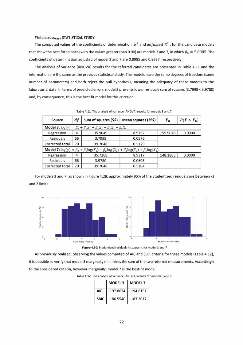
72
𝐘𝐢𝐞𝐥𝐝 𝐬𝐭𝐫𝐞𝐬𝐬𝒓𝒉𝒆𝒐 STATISTICAL STUDY
The computed values of the coefficients of determination 𝑅2 and 𝑎𝑑𝑗𝑢𝑠𝑡𝑒𝑑 𝑅2 , for the candidate models
that show the best fitted ones (with the values greater than 0.90) are models 3 and 7, in which 𝛽0 = 5.8085. The
coefficients of determination adjusted of model 3 and 7 are 0.8985 and 0.8937, respectively.
The analysis of variance (ANOVA) results for the referred candidates are presented in Table 4.11 and the
information are the same as the previous statistical study. The models have the same degrees of freedom (same
number of parameters) and both reject the null hypothesis, meaning the adequacy of these models to the
laboratorial data. In terms of predicted errors, model 3 presents lower residuals sum of squares (3.7999 < 3.9780)
and, by consequence, this is the best fit model for this criterion.
Table 4.11: The analysis of variance (ANOVA) results for models 3 and 7.
Source 𝒅𝒇 Sum of squares (𝑺𝑺) Mean squares (𝑴𝑺) 𝑭𝟎 𝑷(𝑭 > 𝑭𝟎)
Model 3: log (𝑦) = 𝛽0 + 𝛽1𝑋1 + 𝛽2𝑋2 + 𝛽3𝑋3 + 𝛽4𝑋4
Regression 4 35.9049 8.9762 155.9078 0.0000
Residuals 66 3.7999 0.0576
Corrected total 70 39.7048 0.5129
Model 7: log (𝑦) = 𝛽0 + 𝛽1log (𝑋1) + 𝛽2𝑙𝑜𝑔(𝑋2) + 𝛽3log (𝑋3) + 𝛽4log (𝑋4)
Regression 4 35.7268 8.9317 148.1885 0.0000
Residuals 66 3.9780 0.0603
Corrected total 70 39.7048 0.5104
For models 3 and 7, as shown in Figure 4.28, approximately 95% of the Studentized residuals are between -2
and 2 limits.
Figure 4.30: Studentized residuals histograms for model 3 and 7
As previously realized, observing the values computed of AIC and SBIC criteria for these models (Table 4.12),
it is possible so verify that model 3 marginally minimizes the sum of the two referred measurements. Accordingly
to the considered criteria, however marginally, model 7 is the best-fit model.
Table 4.12: The analysis of variance (ANOVA) results for models 3 and 7.
MODEL 3 MODEL 7
AIC -197.8674 -194.6151
SBIC -186.5540 -183.3017
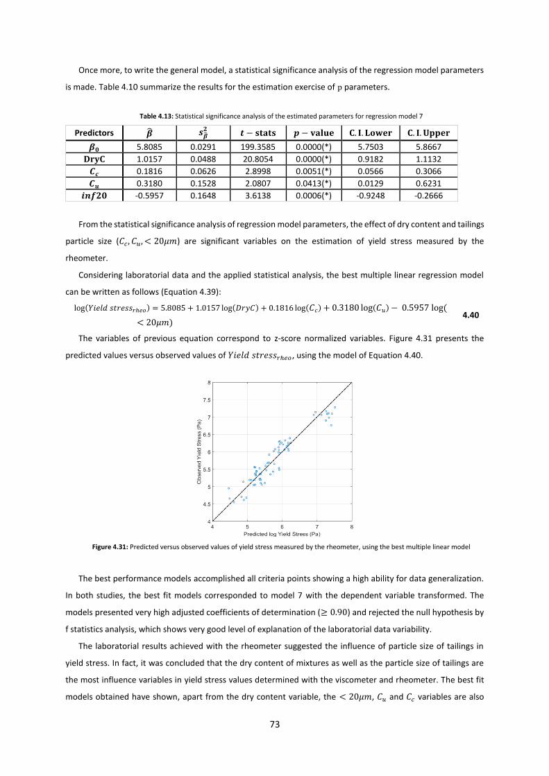
73
Once more, to write the general model, a statistical significance analysis of the regression model parameters
is made. Table 4.10 summarize the results for the estimation exercise of p parameters.
Table 4.13: Statistical significance analysis of the estimated parameters for regression model 7
Predictors �̂� 𝒔�̂�𝟐 𝒕 − 𝐬𝐭𝐚𝐭𝐬 𝒑 − 𝐯𝐚𝐥𝐮𝐞 𝐂. 𝐈. 𝐋𝐨𝐰𝐞𝐫 𝐂. 𝐈. 𝐔𝐩𝐩𝐞𝐫
𝜷𝟎 5.8085 0.0291 199.3585 0.0000(*) 5.7503 5.8667
𝐃𝐫𝐲𝐂 1.0157 0.0488 20.8054 0.0000(*) 0.9182 1.1132
𝑪𝒄 0.1816 0.0626 2.8998 0.0051(*) 0.0566 0.3066
𝑪𝒖 0.3180 0.1528 2.0807 0.0413(*) 0.0129 0.6231
𝒊𝒏𝒇𝟐𝟎 -0.5957 0.1648 3.6138 0.0006(*) -0.9248 -0.2666
From the statistical significance analysis of regression model parameters, the effect of dry content and tailings
particle size (𝐶𝑐, 𝐶𝑢, < 20𝜇𝑚) are significant variables on the estimation of yield stress measured by the
rheometer.
Considering laboratorial data and the applied statistical analysis, the best multiple linear regression model
can be written as follows (Equation 4.39):
log(𝑌𝑖𝑒𝑙𝑑 𝑠𝑡𝑟𝑒𝑠𝑠𝑟ℎ𝑒𝑜) = 5.8085 + 1.0157 log(𝐷𝑟𝑦𝐶) + 0.1816 log(𝐶𝑐) + 0.3180 log(𝐶𝑢) − 0.5957 log (
< 20𝜇𝑚) 4.40
The variables of previous equation correspond to z-score normalized variables. Figure 4.31 presents the
predicted values versus observed values of 𝑌𝑖𝑒𝑙𝑑 𝑠𝑡𝑟𝑒𝑠𝑠𝑟ℎ𝑒𝑜, using the model of Equation 4.40.
Figure 4.31: Predicted versus observed values of yield stress measured by the rheometer, using the best multiple linear model
The best performance models accomplished all criteria points showing a high ability for data generalization.
In both studies, the best fit models corresponded to model 7 with the dependent variable transformed. The
models presented very high adjusted coefficients of determination (≥ 0.90) and rejected the null hypothesis by
f statistics analysis, which shows very good level of explanation of the laboratorial data variability.
The laboratorial results achieved with the rheometer suggested the influence of particle size of tailings in
yield stress. In fact, it was concluded that the dry content of mixtures as well as the particle size of tailings are
the most influence variables in yield stress values determined with the viscometer and rheometer. The best fit
models obtained have shown, apart from the dry content variable, the < 20𝜇𝑚, 𝐶𝑢 and 𝐶𝑐 variables are also

74
significant predictors of yield stress values recorded with the rheometer. This means the percentage of fine
particles, here expressed by the standard reference of granulometry (the material passing under 20 𝜇𝑚) and the
curvature of the particle size distribution of the tailings are very meaningful variables to the rheology of paste
fill.
Therefore, the conclusions made based on experimental data were statistically corroborated and the
influence of tailings granulometry on the rheology of paste fill mixtures proved.

75
CHAPTER 5. CONCLUSION AND RECOMMENDATIONS
5.1 Conclusion
This dissertation is based on an experimental work with the objective of studying the rheology of two case
studies: the paste fill of the Zinkgruvan and Neves-Corvo mines.
It was concluded that rheological characterisation of fresh paste fill mixture is a complex and challenging task,
due to a large number of variables. Different test methods were chosen from a series available techniques
commonly used for this type of measurement, as well as an adoption of other methods normally applied to study
materials such as cement mortar (flow table spread) and soils (fall cone equipment). The sampling of tailings, the
specimen’s preparation and paste mixing procedures were based on a combination of knowledge and practical
information. This is a complex exercise due to numerous physical and chemical/mineralogical factors. The
samples of both mines were tailings filter cake, without a constant water content. The division of the tailings in
bags, with each bag corresponding to a sample for producing one mixture was the best way identified for dealing
with the material, allowing a more accurate determination of tailings water content.
To produce the mixtures, a decision was made to use the same type of cement as that applied in Neves-Corvo
paste backfill and tap water. In preparing samples for testing, it is important to use site or process water, as water
quality can significantly affect the rheological characteristics of the tailings, particularly if clays are present (Sofra,
2017). However, the effect of industrial water, from both sites, on the rheology of each mixture was outside of
the scope of this work. Therefore, tap water was used and the quantity of cement was fixed at 4% for all mixtures.
The results obtained with the viscometer and the rheometer, using the vane technique, showed that the yield
stress range for Zinkgruvan and Somincor mixtures was different. Various explanations were put forward for this,
starting with the different rotational speeds of both pieces of equipment. Furthermore, it was found that
different variables/parameters influenced both yield stresses, in particular, the dry content of mixtures and the
physical properties of tailings. To confirm, mathematically, these assumptions, two statistical studies based on
multiple linear regression models were done in order to predict both yield stresses measured by the viscometer
and rheometer (dependent variable) of all mixtures as a function of quantitative predictors (the percentage of
material passing under 20 𝜇𝑚, the uniformity coefficient (𝐶𝑢) and the coefficient of gradation (𝐶𝑐), obtained in
the experimental work. The best models proved these assumptions, showing a perfect agreement of the
experimental data obtained.
From dry contents and yield stress values, correlations were made with the other test methods: slump, flow
table and fall cone. One of the goals of this work was to verify the differences in values obtained with the
rheometer and viscometer, at different rotational speeds, and how they correlate/fit with all the methods. Every
material also exhibits particular rheological behaviour and it is therefore interesting to evaluate the quality of
the results obtained with all the test methods and analyse their performances with these two different materials.
Moreover, these expressions were achieved with other materials (concrete, for example), which cannot be
associated with paste fill. Apart from this, some previous studies showed poor correlations, usually
overestimated, between the yield stress values determined by vane methodology and calculated by these
formulations.

76
Of all the test methods, the measurement that showed the worst results was the initial diameter of the flow
table. This measure was not able to characterise mixtures with high dry contents, keeping a diameter that
remained similar to the cone mould Apart from this, all the methods were able to evaluate the difference
between mix designs and obtain good correlations with yield stress. Nevertheless, observing Table 4.6, the yield
stress values recorded by the viscometer present very high coefficients of determination (>0.91) with all
methodologies. The flow table (final diameter) and the 300 fall cone presented the best performances. In the
comparison between both mine mixtures, the best results were achieved with the Neves-Corvo tailings.
The experimental testing programme has proven to be able both to test the rheology of paste fill, particularly
the measurement of yield stress, and provide valid and meaningful data about the influence of solids
concentration and particle size on the behaviour of paste fill. It can be concluded that the methodology utilised
in this work can be used to other case studies.
As previously explained, the rheological study of paste fill is essential not only for the implementation of this
backfill technology but also for quality control of running production systems. With this in mind and knowing the
differences in yield stress values obtained with both equipment, it is possible to identify, in both scenarios, what
would be the best solution for measuring this rheological property.
To design and implement a paste backfill system (paste plant and pipeline reticulation) it is very important to
know the shear stress needed to start moving the paste fill and to what degree the variability of tailings
properties (associated with the ore bodies) affects these properties. Thus, as the rheometer can record the values
at lower speeds, the yield stress values measured are closer to the transition from static to dynamic state of the
material, providing a more reliable shear stress value that corresponds to the breaking of the internal structure
of the paste mixture. Furthermore, at this low rotational speed it was confirmed that the concentration of solids
and the particle size of tailings have a major effect on paste fill rheology. As such, the rheometer provides valid
and useful data, such as the yield stress profiles (as a function of solids concentration and cement content), that
are the most important data set for design and operation of paste systems.
Alternatively, the viscometer is a simple, low-cost and portable (smaller and lighter) equipment, presenting
better correlations with the other experimental technologies. The viscometer is very suitable equipment to
controlling the quality of paste fill, by measuring not only the yield stress but also the apparent viscosity. It is also
useful to simplify research and development projects for new mix designs/compositions.
The fall cone test adopted for this experimental work turned out to be the methodology that performed best,
with very good correlation with the dry content of the mixtures and the yield stress values achieved by the
viscometer and rheometer. The weight and geometry of the cones combined with the release time have proven
to be a successful procedure for measuring paste fill rheology, and thus represent one of this work’s major
contributions. This equipment can become a simple, inexpensive, convenient and fast method of determining
the yield stress, ideal for quality control and/or rapid on-site measurements.
At a time where environmental pressures are increasing and there is a constant drive to turn mining in a
more sustainable industry, in all aspects, rheology can play an essential role in better understanding and dealing
with thickened tailings. However, it is necessary to bring together scientific and practical knowledge, which is
currently scattered across consulting companies, the scientific community and the mining industry and to enable
77
on-site measurements in order to achieve new and significant improvements in mining backfill. The necessity of
standard methods to test paste fill rheology is a reflex of this lack of synergies. The opportunity to visit the
Zinkgruvan and Neves-Corvo paste plants and work with Sika make me realise the need for the standardisation
of these tests for companies that are dealing with the same subject and sharing the same issues/situations.
After carrying out this work, it was easier to see the changeability of the results obtained with different
techniques and thus the necessity of creating a standard experimental testing programme to study paste fill
worldwide.
In conclusion, the objectives established for this dissertation were completely achieved, as the final learning
outcomes represent a significant contribution to the rheological study of paste backfill. I am certain that the
experimental testing programme and the new technical approaches developed in this study can be applied in
practice and further improved in future research projects.
5.2 Recommendations
From the outcomes of this experimental work and the knowledge acquired by observation and
experimentation on mine sites, some topics/ideas have emerged for future research work.
Firstly, there is experimentation with different mix designs using the same mine tailings. It is necessary to
know the influence of cement proportions on the workability of paste fill, namely the yield stress property, by
drawing yield stress versus cement concentration profiles. For example, in a cement reduction study with the
objective of reducing the cost of paste fill production, mixtures could be tested with the addition of other binders,
such as fly ash, at different proportions. Furthermore, it would be of interest to evaluate the effect of industrial
water (used in both paste plants) on these new mixtures. The influence of water chemistry has already been
demonstrated in previous works, but due to the uniqueness of each case study, this effect should be retained for
these two paste fills.
Due to the changeability of tailings properties, which can vary significantly in both location and depth within
a particular ore body, a campaign of tailings sampling should be done at different times to produce and test
similar mix designs. This should enable a balance/estimation study of paste rheology, in particular yield stress
property, on a larger scale.
Moreover, this work was mainly focused on determining the yield stress of mixtures that have just been
produced. A dynamic analysis of rheological behaviour of these mixtures would definitely be worthwhile in order
to understand how these materials behave at different rotational velocities. Using the vane technique (with a
viscometer or a rheometer) it is possible to set a crescent rotational speed ramp to observe the peaks in viscosity
and shear stress and verify the time dependency of each mixture. Additionally, it could be interesting to analyse
the yield stress of these materials at several stages of curing, thus measuring the yield stress at different times
and conditions. This could provide information about the shear stress needed to start the paste flowing through
a pipe, after some stoppage.
Another necessary and challenging task is measuring the scaling factor between laboratorial testing results
and on-site measurements. One possibility for how to study these differences is to sample tailings filter cake and
test the fresh paste fill that is being produced at the plant at the same time. It would be possible to reproduce

78
and test similar paste mixture in the lab, using the tailings collected, the industrial water and the mix design of
the paste that is being produced at the plant. By comparing the results it should be possible to determine the
scale effect.
Finally, because of the remarkable results obtained with the fall cone test and taking into account the
performance of this equipment with this type of material, there is the possibility of using this methodology to
study not only fresh paste fill mixtures but also the rheology of tailings in different phases of paste production.
For example, it could provide a useful testing tool for determining the water content of tailings filter cake and
thus inspecting/assessing the efficiency/productivity of filters.

79
REFERENCES
ATA SCIENTIFIC (2012), Understanding yield stress measurements, Malvern Instruments Worldwide.
BARNES, H. HUTTON, J. WALTERS, S. (1993), An introduction to Rheology, Elsevier.
BELEM, T. BENZAAZOUA, M. (2008), Predictive models for prefeasibility cemented paste backfill mix design, Post-
Mining, February 6-8, Nancy, France.
BELEM T, BENZAAZOUA M (2008), Design and Application of Underground Mine Paste Backfill Technology,
Geotech Geol Eng 26:175.
BGUYEN, Q. BOGER, D.V. (1998), Application of rheology to solving tailings disposal problems, Int. J. Miner.
Process 54, 217-233.
BOGER D (2009), Rheology and the resource industries, Chemical Engineering Science 64 4525-4536.
BOGER D. (2006), Rheological Concepts, Paste and Thickened Tailings – A Guide (2nd edition), chapter 3, Australia
Centre for Geomechanics.
BROOKFIELD (2016), More solutions to sticky problems, Brookfield engineering laboratories inc.
COOKE, R. (2007), Backfill pipeline distribution systems – design methodology review, Minefill paper 20.
FALL, M. BENZAAZOUA, M. SAA, E. (2006), Mix proportioning of underground cemented tailings backfill,
Tunnelling and Underground Space Technology 23 80-90.
FERRARIS, C. (1999), Measurement of Rheological Properties of High Performance Concrete: State of the Art
Report, Journal of Research of the National Institute of Standards and Technology, Vol. 104, No. 5 Sep-Oct
1999.
GRICE, T. (1998), Underground mining with Backfill, Mine tailings disposal systems, Brisbane.
HE, M. WANG, Y. FORSSBERG, E. (2004), Slurry rheology in wet ultrafine grinding of industrial minerals: a review,
Powder Technology 147 94-112.
KLEIN, B. HALLBOM, D. (2014), Rheology of paste and thickened tailings, Vancouver, Canada.
MOLLER, C. MEWIS, J. BONN, D. (2006), Yield stress and thixotropy: on the difficulty of measuring yield stresses
in practice, Soft Matter 2, 274-283.
NGUYEN, Q. AKROYD, T. KEE, D. ZHU, L. (2005), Yield stress measurements in suspensions: an inter-laboratory
study, Korea-Australia Rheology Journal Vo. 18, No. 1, March 2006, pp. 15-25.
PANEIRO, G. Durão, F. Costa e Silva, M. Neves, P. (2015), Prediction of ground vibration amplitudes due to urban
railway traffic using quantitative and qualitative field data, Transportation Research Part D 40 1-13.
PATERSON, A.J.C. (2011), The pipeline transport of high density slurries – a historical review of past mistakes,
lessons learned and current technologies, Paste 2011, Perth, Australia.
POTVIN Y, THOMAS E, FOURIE, A (2014), Handbook on Mine fill, chapter 6, Australia Centre for Geomechanics.
SAEBIMOGHADDAM, A. (2005), Rheological yield stress measurement of mine paste fill material, McGill
University, Montreal, Canada.
SIMON, D. GRABINSKY, M. (2012), Apparent yield stress measurement in cemented paste backfill, International
Journal of Mining, Reclamation and Environment, Vol. 27, No. 4, 231-256.
WANG, Y. (2012), The effect of solid components on the rheological and mechanical properties of cemented paste
backfill, Minerals Engineering August 2012.

80
YILMAZ, E. FALL, M. (2017), Paste tailings management, Springer.
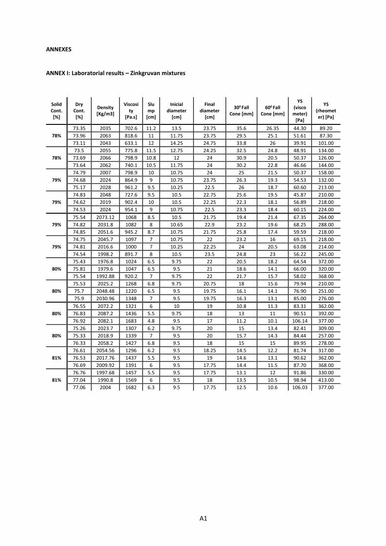
A1
ANNEXES
ANNEX I: Laboratorial results – Zinkgruvan mixtures
Solid Cont. [%]
Dry Cont. [%]
Density [Kg/m3]
Viscosity
[Pa.s]
Slump
[cm]
Inicial diameter
[cm]
Final diameter
[cm]
300 Fall Cone [mm]
600 Fall Cone [mm]
YS (viscometer)
[Pa]
YS (rheometer) [Pa]
78%
73.35 2035 702.6 11.2 13.5 23.75 35.6 26.35 44.30 89.20
73.96 2063 818.6 11 11.75 23.75 29.5 25.1 51.61 87.30
73.11 2043 633.1 12 14.25 24.75 33.8 26 39.91 101.00
78%
73.5 2055 775.8 11.5 12.75 24.25 32.5 24.8 48.91 134.00
73.69 2066 798.9 10.8 12 24 30.9 20.5 50.37 126.00
73.64 2062 740.1 10.5 11.75 24 30.2 22.8 46.66 144.00
79%
74.79 2007 798.9 10 10.75 24 25 21.5 50.37 158.00
74.68 2024 864.9 9 10.75 23.75 26.3 19.3 54.53 132.00
75.17 2028 961.2 9.5 10.25 22.5 26 18.7 60.60 213.00
79%
74.83 2048 727.6 9.5 10.5 22.75 25.6 19.5 45.87 210.00
74.62 2019 902.4 10 10.5 22.25 22.3 18.1 56.89 218.00
74.53 2024 954.1 9 10.75 22.5 23.3 18.4 60.15 224.00
79%
75.54 2073.12 1068 8.5 10.5 21.75 19.4 21.4 67.35 264.00
74.82 2031.8 1082 8 10.65 22.9 23.2 19.6 68.25 288.00
74.85 2051.6 945.2 8.7 10.75 21.75 25.8 17.4 59.59 218.00
79%
74.75 2045.7 1097 7 10.75 22 23.2 16 69.15 218.00
74.81 2016.6 1000 7 10.25 22.25 24 20.5 63.08 214.00
74.54 1998.2 891.7 8 10.5 23.5 24.8 23 56.22 245.00
80%
75.43 1976.8 1024 6.5 9.75 22 20.5 18.2 64.54 372.00
75.81 1979.6 1047 6.5 9.5 21 18.6 14.1 66.00 320.00
75.54 1992.88 920.2 7 9.75 22 21.7 15.7 58.02 368.00
80%
75.53 2025.2 1268 6.8 9.75 20.75 18 15.6 79.94 210.00
75.7 2048.48 1220 6.5 9.5 19.75 16.1 14.1 76.90 251.00
75.9 2030.96 1348 7 9.5 19.75 16.3 13.1 85.00 276.00
80%
76.55 2072.2 1321 6 10 19 10.8 11.3 83.31 362.00
76.83 2087.2 1436 5.5 9.75 18 13 11 90.51 392.00
76.92 2082.1 1683 4.8 9.5 17 11.2 10.1 106.14 377.00
80%
75.26 2023.7 1307 6.2 9.75 20 15 13.4 82.41 309.00
75.33 2018.9 1339 7 9.5 20 15.7 14.3 84.44 257.00
76.33 2058.2 1427 6.8 9.5 18 15 15 89.95 278.00
81%
76.61 2054.56 1296 6.2 9.5 18.25 14.5 12.2 81.74 317.00
76.53 2017.76 1437 5.5 9.5 19 14.6 13.1 90.62 362.00
76.69 2009.92 1391 6 9.5 17.75 14.4 11.5 87.70 368.00
81%
76.76 1997.68 1457 5.5 9.5 17.75 13.1 12 91.86 330.00
77.04 1990.8 1569 6 9.5 18 13.5 10.5 98.94 413.00
77.06 2004 1682 6.3 9.5 17.75 12.5 10.6 106.03 377.00

A2
ANNEX I: Laboratorial results – Neves-Corvo mixtures
Solid Cont. [%]
Dry Cont. [%]
Density [Kg/m3]
Viscosity
[Pa.s]
Slump
[cm]
Inicial diameter
[cm]
Final diameter
[cm]
300 Fall Cone [mm]
600 Fall Cone [mm]
YS (viscometer)
[Pa]
YS (rheometer) [Pa]
78%
76.53 2365.52 1058 12.5 17.75 24.5 36.5 24.9 65.67 186.00
77.67 2374.64 1874 12 12.75 23.25 29.6 21.1 116.35 182.00
77.66 2383.36 2584 12 12.5 22 29 20.4 160.43 185.00
78%
76.73 2412.8 1172 12 18 25 36.5 24.8 72.72 164.00
76.74 2395.2 1193 12.5 18 25.25 36 26 74.04 183.00
77.12 2380.32 1413 11.5 17.5 24.5 33.8 24.4 87.70 184.00
78%
76.41 2358.96 1151 12.5 18.25 25 36.1 24.5 71.40 178.00
77.04 2335.84 1299 12 15.5 23.75 33.6 22.4 80.65 190.00
77.29 2414.08 1611 11 14.25 22.75 31.3 20.2 100.05 194.00
78%
76.66 2355.2 1051 13 18 25 34 23.5 65.23 188.00
76.8 2377.68 1051 12.5 17.75 25.5 34.1 24.5 65.23 190.00
76.92 2402.16 1214 12 17.5 25 36.5 24.8 75.36 193.00
80%
78.57 2450.64 2393 10.5 10.75 21.5 26.6 17.2 148.53 383.00
79.26 2918 2918 9.5 10 20.75 23 16.2 181.14 393.00
79.32 2426.64 3259 8.5 10 20 20 15.6 202.29 369.00
80%
78.63 2432.96 2549 10 10.25 21.5 25.5 21.5 158.22 485.00
78.75 2421.36 2698 9 10 21 26.7 18.5 167.48 479.00
79.13 2395.12 2975 7.5 9.75 21 23.5 16.6 184.67 510.00
80%
78.69 2434.48 2535 10 10.25 20.75 26.6 18.5 157.34 430.00
79.01 2408.88 2684 8 10 21 22.5 18.5 166.60 479.00
79.3 2425.44 2876 7 9.5 20 22.1 12.2 178.49 439.00
80%
78.52 2428.16 2123 11 11 22 27.9 14.5 131.78 459.00
78.75 2438.4 2684 10 10.75 21.25 28.1 18.5 166.60 477.00
79.05 2435.28 2968 10 10.5 21.75 23.8 16.8 184.22 505.00
82%
81.12 2574.72 14190 5 9.25 16.25 11.8 10.3 345.53 997.00
81.3 2456.96 6319 4.5 9 16 9 8 392.25 1050.00
82%
80.62 2450.24 5332 6 9.5 18.25 16.5 11 330.99 1410.00
80.99 2442.88 5055 5 9 18 11.1 8.9 313.80 1240.00
81.23 2481.44 6042 4 9 17 9.3 8 375.06 1430.00
82%
80.82 2474.96 5119 5 9.5 17.5 11.8 10.2 317.77 1540.00
80.31 2566.8 6063 4 9 16.75 9.8 6.7 376.38 1650.00
81.07 2408.72 6433 4 9.25 17 11 7.5 399.30 1470.00
82%
80.72 2509.28 5297 4.5 9.5 19 15 10.6 328.78 1520.00
80.69 2494.56 5708 5 9.25 19 13.5 9.6 354.35 1680.00
81.12 2543.04 5460 4 9 18 12.3 9.2 338.92 1840.00